From O(3) to Cubic CFT: Conformal Perturbation and the Large Charge Sector

Abstract

The Cubic CFT can be understood as the O(3) invariant CFT perturbed by a slightly relevant operator. In this paper, we use conformal perturbation theory together with the conformal data of the O(3) vector model to compute the anomalous dimension of scalar bilinear operators of the Cubic CFT. When the $Z_{2}$ symmetry that flips the signs of $\phi_{i}$ is gauged, the Cubic model describes a certain phase transition of a quantum dimer model. The scalar bilinear operators are the order parameters of this phase transition. Based on the conformal data of the O(3) CFT, we determine the correction to the critical exponent as $\eta_{*}^{Cubic}-\eta_{*}^{O(3)}\approx-0.0215(49)$. The O(3) data is obtained using the numerical conformal bootstrap method to study all four-point correlators involving the four operators: $v=\phi_{i}$, $s=\sum_{i}\phi_{i}\phi_{i}$ and the leading scalar operators with O(3) isospin $j=2$ and 4. According to large charge effective theory, the leading operator with charge $Q$ has scaling dimension $\Delta_{Q}=c_{3/2}Q^{3/2}+c_{1/2}Q^{1/2}$. We find a good match with this prediction up to isospin $j=6$ for spin 0 and 2 and measured the coefficients $c_{3/2}$ and $c_{1/2}$.

1 Introduction

The $O(3)$ vector model deformed by the cubic anisotropic term,

$$S=\int dtdx^{2}\sum_{i=1}^{3}(\partial_{\mu}\phi_{i})^{2}+r\sum_{i=1}^{3}\phi_{i}^{2}+u(\sum_{i=1}^{3}\phi_{i}\phi_{i})^{2}+v_{4}\sum_{i=1}^{3}(\phi_{i})^{4},$$ (1.1)

was first proposed in aharony1973critical to describe the crystal structural phase transition on perovskite materials. Over the years, the model has attracted the attention of physicists from different backgrounds. In particular, an interesting question is to identify the most stable fixed point of (1.1) under renormalization group flow. The question was under debate for many years (as was reviewed in Aharony:2022ajv ) until recently. The lattice Monte Carlo simulation result in PhysRevB.84.125136 ; Hasenbusch:2022zur ; Hasenbusch:2023fmn , the perturbative quantum field thory KLEINERT1995284 ; PhysRevB.61.15136 ; Adzhemyan:2019gvv and the conformal bootstrap result in Chester:2020iyt all claim that the Cubic fixed point with non-vanishing coupling $v_{4}$ (instead of the $O(3)$ invariant fixed point) is the most stable one. The stability of the fixed points is closely related to the scaling dimension of the operator that introduces the cubic anisotropy, which belongs to the $j=4$ irreducible representation of O(3). The conformal bootstrap result Chester:2020iyt provides rigorous proof that $\Delta_{O}<3$ at the $O(3)$ fixed point. This means that the Cubic model is in a new universality class.

Recently, the quantum Monte Carlo simulation in Yan:2022zwt shows that the Cubic models also describe a second-order quantum phase transition of a quantum dimer model on a triangular lattice, building on earlier studies of the model such as in PhysRevLett.61.2376 ; PhysRevB.92.075141 ; moessner2001resonating ; PhysRevB.99.165135 ; yan2021topological ; Yan_2022 . The renormalization group flow structure of (1.1) plays an important role in understanding the phase diagram of the quantum dimer model.

Besides the above-mentioned connections to interesting phase transitions, the importance of the model (1.1) can be seen from a different angle. Consider $N$ scalar fields coupled together, to study possible conformal field theories, one can consider perturbation theory in $4-\epsilon$ expansion. Requiring the CFTs to have a single relevant operator, which corresponds to imposing the physical condition so that they correspond to critical points (rather than tri-critical points), the classification work of PhysRevB.10.892 ; PhysRevB.31.7171 ; Rong:2023xhz shows that the list of such CFTs is very short, in particular when $N$ is small. If one chooses to extrapolate the result to $2+1$ dimensions, this means scalar universality classes that can be reached without fine-tuning are very limited. The Cubic CFTs are valuable members of such a list.

Ever since the seminal work of Rattazzi:2008pe , the conformal bootstrap method Poland:2018epd has become one of the most successful methods in studying conformal field theories in 2+1 dimensions El-Showk:2012cjh ; El-Showk:2014dwa ; Kos:2014bka ; Kos:2013tga ; Kos:2015mba ; Chester:2020iyt ; Chester:2019ifh ; Rong:2018okz ; Atanasov:2018kqw ; Kos:2016ysd . However, even though there were some attempts Rong:2017cow ; Stergiou:2018gjj ; Kousvos:2018rhl , the direct isolation of Cubic CFTs and the precise determination of their critical exponents remain elusive in numerical conformal bootstrap. Partially motivated by this goal, the model has been revisited recently using various perturbative methods Antipin:2019vdg ; Bednyakov:2023lfj ; Binder:2021vep .

In this paper, we will use conformal perturbation theory together with the conformal data of the O(3) vector model to calculate the scaling dimensions of scalar bi-linear operators in the Cubic CFT. These operators are in fact the order parameter of the phase transition of the quantum dimer model Yan:2022zwt ; Ran:2023wju . More precisely speaking, the low energy effective action that describes the phase transition is given by (1.1) coupled to a $Z_{2}$ gauge theory. The $Z_{2}$ symmetry that was gauged flips the sign of all three $\phi_{i}$’s. Since the $\phi_{i}$ operator is not gauge invariant, they can not be the order parameter of the lattice model. The order parameters of the phase transition are instead composite operators $\phi_{1}\phi_{2}$, $\phi_{2}\phi_{3}$, and $\phi_{1}\phi_{3}$. Such $Z_{2}$ gauged CFTs are usually denoted with a “*” and have been studied numerically before, the O(2)* universality was observed in sachdev1999translational ; huh2011vison ; YCWang2018 , while the O(4)* universality was studied in moessner2001ising ; PhysRevLett.86.1881 ; yan2021topological . In anticipation of future computer or even experimental measurement, it is therefore interesting to calculate the critical exponents

$$\eta_{*}=2\Delta_{\phi_{1}\phi_{2}}-1.$$

In conformal perturbation theory, the difference of the critical exponents $\eta_{*}$ between the Cubic CFT and the O(3) CFT is the leading order in the perturbation parameter $\delta$, which is related to the scaling dimension of the leading scalar operator in the $j=4$ irreducible representation of O(3) by $\delta=3-\Delta_{t_{4}}\approx 0.01$ Chester:2020iyt ; Hasenbusch:2022zur ; Hasenbusch:2023fmn . The $\eta_{*}$ difference also depends on the OPE coefficient ratio $\alpha_{ttt_{4}}/\alpha_{t_{4}t_{4}t_{4}}$. The symbol $T^{(j)}$ here denotes the leading scalar operator in the isospin $j$ irreducible representation of O(3). To calculate $\alpha_{t_{4}t_{4}t_{4}}$, we set up, for the first time, a bootstrap program involving all four point correlators of $v=\phi_{i}$, $s=\sum_{i}\phi_{i}\phi_{i}$, $t$ and $t_{4}$. Our result shows that the $\eta_{*}$ difference between the Cubic CFT and the O(3) CFT start at two decimal places,

$$\eta_{*}^{Cubic}-\eta_{*}^{O(3)}\approx-0.0215(49).$$ (1.2)

Together with current most precise determination Chester:2020iyt of $\eta_{*}^{O(3)}=2\Delta_{T}-(d-2)=1.41908(64)$, we get $\eta_{*}^{Cubic}\approx 1.398$. Even though it seems challenging to observe such a difference in experiments, the recent studies in Hasenbusch:2022zur ; Hasenbusch:2023fmn suggest that the two CFTs are indeed distinguishable in Monte Carlo simulations. (In particular, critical exponents $\nu$ of the two CFTs were shown to be different Hasenbusch:2023fmn .)

Our numerical bootstrap setup allows us to access many operators with high $O(3)$ representations. This allows us to check against the prediction of the scaling dimension of the large charge operators predicted by the large quantum charge effective theory Hellerman:2015nra ; Monin:2016jmo ; Alvarez-Gaume:2016vff ; PhysRevLett.120.061603 ; PhysRevLett.123.051603 ; Alvarez-Gaume:2019biu , which states

$$\Delta_{Q}=c_{3/2}Q^{3/2}+c_{1/2}Q^{1/2}-0.094+\sqrt{\frac{l(l+1)}{2}}$$ (1.3)

Reading the spectra of operators from extremal functional, we get

$$c_{1/2}=0.304(35),\quad c_{3/2}=0.315(7)$$ (1.4)

which are universal for all models that realize the O(3) universality class.

2 The Cubic CFT from conformal perturbation

As discussed in Komargodski:2016auf ; Behan:2017emf ; Behan:2017dwr , when a CFT is perturbed by an operator,

$$\int dx^{2}gO(x),$$ (2.1)

one may consider the renormalization group flow induced by such as perturbation. The operator $O$ satisfies the normalization

$$\langle O(x_{1})O(x_{2})\rangle=\frac{1}{x_{12}^{2\Delta_{O}}},$$ (2.2)

If $\Delta_{O}=3-\delta$, the beta function is given by

$$\beta(g)=\frac{dg}{d\mu}=-\delta g-\frac{1}{2}C_{OOO}S_{d-1}g^{2}+\mathcal{O}(g^{3}).$$ (2.3)

$C_{OOO}$ is the OPE coefficient, and $S_{d-1}$ is the volume of unit (d-1)-sphere. The RG flow has an Infra-red fixed point when $C_{OOO}>0$ and $\delta>0$. One can read out the scaling dimension of the $O$ operator in the new fixed point, which corresponds to the $\omega$ critical exponent

$$\omega=\frac{\partial\beta(g)}{\partial g}\bigg{|}_{g=g_{*}}=\delta.$$ (2.4)

Notice such a relation was shown to hold very precisely for the Cubic/O(3) CFT pair in Hasenbusch:2023fmn . Take another operator $\phi(x)$ (different from $O(x)$), again satisfying the normalization (2.2), its anomalous dimension is given by

$$\gamma_{\phi}=\frac{2C_{\phi\phi O}}{C_{OOO}}\delta+\mathcal{O}(\delta^{2}).$$ (2.5)

Higher order terms of (2.3) and (2.5) depend on the renormalization scheme. If the leading order vanishes (due to symmetry reasons), the next order terms are also scheme-independent.

The operators of a CFT with O(3) symmetry are normalized as

$$\langle O^{(\Delta,l,j_{1})}{}_{\alpha}(x_{1},\xi_{1})O^{(\Delta,l,j_{2})}_{\beta}(x_{2},\xi_{2})\rangle=\delta_{j_{1},j_{2}}G^{(j)}_{\alpha\beta}\frac{(I_{\mu\nu}(x_{12})\xi_{1}^{\mu}\xi_{2}^{\nu})^{l}-trace}{x_{12}^{2\Delta}},\quad I_{\mu\nu}(x)=\eta_{\mu\nu}-2\frac{x_{\mu}x_{\nu}}{x^{2}}.$$ (2.6)

Here $\xi^{\mu}$ is auxiliary null vectors. $j$ labels the O(3) representation, while $l$ denote the spin of the operator.The matrix $G^{(j)}_{ab}$ is defined in (A.7) through Clebsch–Gordan coefficients.

The operator product expansion of two scalar operators is defined as

$$O^{(j_{1})}_{1,a}(x_{1})\times O^{(j_{2})}_{2,b}(x_{2})\sim\sum_{j}\alpha_{123}^{(j_{1},j_{2},j_{3})}X^{(j_{1},j_{2},j_{3})}_{abe}G^{(j)ef}C_{\Delta,l,\mu_{1}\ldots\mu_{l}}(x_{12}^{\mu},\partial_{2,\mu})O^{\Delta,l,\mu_{1}\ldots\mu_{l}}_{3,f}(x_{2}).$$ (2.7)

This implies the 3pt function be

$$\langle O^{(j_{1})}_{1,a}(x_{1})O^{(j_{2})}_{2,b}(x_{2})O^{(\Delta,l,j)}_{3,c}(x_{3},\xi_{3})\rangle=\alpha_{123}^{(j_{1},j_{2},j_{3})}X^{(j_{1},j_{2},j_{3})}_{abc}\frac{(Z^{\mu}\xi_{3,\mu})^{l}}{x_{12}^{\Delta_{1}+\Delta_{2}-\Delta_{3}}x_{23}^{\Delta_{2}+\Delta_{3}-\Delta_{1}}x_{13}^{\Delta_{1}+\Delta_{3}-\Delta_{2}}},$$ (2.8)

with

$$Z^{\mu}=\frac{x_{13}^{\mu}}{x_{13}^{2}}-\frac{x_{12}^{\mu}}{x_{12}^{2}}.$$ (2.9)

The invariant tensor $X^{(r,s,t)}_{abc}$ is defined in (A.9), which is proportional to the Clebsch–Gordan coefficient. We have provided a file containing all the conformal data of the O(3) CFT available for our bootstrap calculation. The above definitions for two and three-point functions are equivalent to saying that our conformal block follows the convention of the first line of Table I in Poland:2018epd . Among the operators of the O(3) CFT, there are two operators that are relevant for our conformal perturbation calculation. They are the lowest dimension scalar operators in the $j=2$ and $j=4$ channel, we will denote them as $t$ and $t_{4}$.

We deform the O(3) CFT by the operator

$$M(x)=\sqrt{\frac{5}{6}}Q^{ijkl}e^{(4)a}_{ijkl}(t_{4})_{a}(x).$$ (2.10)

The tensor $e^{(4)a}_{ijkl}$ is defined in (A.6), with $a=-4,...4$ and $i,j,k,l=1,..3$. This is used to change the basis from rank-4 symmetric traceless tensor to $J^{2},J_{3}$ eigenstates basis in which the CG coefficients are defined (and used in the bootstrap setup). The tensor

$$Q^{ijkl}=\bigg{\{}\begin{array}[]{l}1,\quad\text{if $i=j=k=l$}\\ 0,\quad\text{otherwise.}\\ \end{array}$$ (2.11)

is invariant under the Cubic group, which indicates the direction along which the O(3) group is broken into its Cubic subgroup. The constant $\sqrt{5/6}$ in (2.10) is chosen such that $M$ satisfies the normalization condition (2.2).

The $j=2$ irrep of O(3), when decomposed into irreps of the Cubic group is given by the following branching rule:

$$(j=2)\longrightarrow w+t^{\prime}.$$ (2.12)

The order parameter of the Cubic^∗ is defined as

$$W(x)=\frac{1}{\sqrt{2}}w^{ij}e^{(2)a}_{ij}t_{a}(x).$$ (2.13)

with $e^{(2)a}_{ij}$ defined in (A.6). The tensor

$$w^{ij}=\left(\begin{array}[]{ccc}0&1&0\\ 1&0&0\\ 0&0&0\\ \end{array}\right)$$ (2.14)

belong to the “w” irrep. It is also the irreps that the quadratic fields $\{\phi^{1}\phi^{2},\phi^{1}\phi^{3},\phi^{2}\phi^{3}\}$ of (1.1) transforms in. We can also calculate the anomalous dimension of

$$T^{\prime}(x)=\frac{1}{\sqrt{6}}t^{\prime ij}e^{(2)a}_{ij}t_{a}(x).$$ (2.15)

The tensor

$$t^{\prime ij}=\left(\begin{array}[]{ccc}1&0&0\\ 0&1&0\\ 0&0&-2\\ \end{array}\right)$$ (2.16)

transforms $t^{\prime}$ irrep of the Cubic group. In terms of quadratic fields, the two-dimensional irrep is spanned by $(\phi^{1})^{2}+(\phi^{2})^{2}-2(\phi^{3})^{2}$ and $(\phi^{2})^{2}+(\phi^{3})^{2}-2(\phi^{1})^{2}$. The scaling dimension of the $t^{\prime}$ operator controls the crossover critical behavior from the Cubic universality class to the Ising universality class PhysRevLett.33.427 ; Pelissetto:2000ek , which can be realized in the structural phase transition of perovskites muller1975behavior .

Using the above definition, we get that

$$C_{WWM}=-\frac{1}{3}\sqrt{\frac{2}{15}}\alpha_{ttt_{4}},\quad\quad C_{T^{\prime}T^{\prime}M}=\sqrt{\frac{1}{30}}\alpha_{ttt_{4}},$$ (2.17)

and

$$C_{MMM}=\frac{7}{3}\sqrt{\frac{2}{429}}\alpha_{t_{4}t_{4}t_{4}}$$ (2.18)

Clearly, the $\alpha_{t_{4}t_{4}t_{4}}$ OPE coefficients appear in the conformal block expansion of the four-point function of $\langle t_{4}(x_{1})t_{4}(x_{2})t_{4}(x_{3})t_{4}(x_{4})\rangle.$ To get this OPE using conformal bootstrap, we set up a bootstrap program involving all four point correlators of $\phi_{i}$, $S=\sum_{i}\phi_{i}\phi_{i}$, $t$ and $t_{4}$. This is a heavy calculation. We leave the numerical details of the calculation in Appendix B. The bootstrap calculation gives us the OPE ratio

$$\alpha_{ttt_{4}}/\alpha_{t_{4}t_{4}t_{4}}\approx 0.62(14).$$ (2.19)

From these results, we get that

$$\gamma_{W}=2\frac{C_{WWM}}{C_{MMM}}\delta\approx-0.0107(24),\quad\text{and}\quad\gamma_{T^{\prime}}=2\frac{C_{T^{\prime}T^{\prime}M}}{C_{MMM}}\delta\approx 0.0161(36).$$ (2.21)

By plugging $\Delta_{t}=1.20954$ Chester:2020iyt , we get

$$\Delta_{W}\approx 1.1988(24),\quad\text{and}\quad\Delta_{T^{\prime}}\approx 1.2256(36).$$ (2.22)

In terms of the critical exponents $\eta_{*}$, we get (1.2).

3 Large charge operators of the O(3) CFT

Our numerical bootstrap setup allows us to access many operators with high $O(3)$ representations. To be precise, for Lorentzian scalars with $l=even$, operators with $O(3)$ isospin up to $j=8$ appear in our bootstrap setups. The scaling dimension of those operators can be estimated by choosing a feasible point in our setup and using the Extreme Functional Method (EFM) ElShowk:2012hu On the other hand, large quantum charge effective theory Hellerman:2015nra ; Monin:2016jmo ; Alvarez-Gaume:2016vff ; PhysRevLett.120.061603 ; PhysRevLett.123.051603 ; Alvarez-Gaume:2019biu predicts the asymptotic behavior of such operators to be (1.3).

In the case of the O(3) model, one can take $Q=j$. Initially, it was expected that the above formula is valid for when $0\leq l\ll\sqrt{Q}$. The recent Monte Carlo simulation, however, shows that for O(2) and O(4) CFTs, the above asymptotic behavior works even when $Q\sim\mathcal{O}(1)$. In Figure 1, we plot our data against the large charge effective theory, for both $l=0$ and $l=2$ operators. Our results suggest that the large charge formula works even for small charge operators. We remark that this is the first time that (1.3) has been tested for $l\neq 0$. For the charge 8 operators, our value is strongly affected by the sharing effect and unreliable. But it can be improved in the future by increasing $\Lambda$.

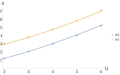
Figure 1: The scaling dimension of large charge spin 0 and spin 2 operators, obtained using the Extremal Functional Method. The curves are obtained by fitting the spin-0 and spin 2 operators against the large charge formula $\Delta_{Q,l=0}=c_{3/2}Q^{3/2}+c_{1/2}Q^{1/2}-0.094$.

Fitting both spin 0 and spin 2 operators’ dimensions by (1.3), we get (1.4). From the figure we observed both sectors match well with the large charge expansion formula.

4 Discussion

Using the conformal data obtained from our conformal bootstrap setup, we can also calculate the perturbation correction to the anomalous dimension of the critical exponents $\eta$ and $\nu$, corresponding to the operators $\phi_{i}$ and $\phi^{2}=\sum_{i}(\phi_{i})^{2}$ of the Cubic CFT. Due to O(3) symmetry, the OPE coefficient $C_{\phi\phi t_{4}}$ and $C_{\phi^{2}\phi^{2}t_{4}}$ both vanish. The conformal perturbation corrections to the scaling dimension of $\phi$ and $\phi^{2}$ start at order $\mathcal{O}(\delta^{2})$, which should also be very small. This was first observed in an earlier field theoretical calculation calabrese2003randomly , and confirmed using Monte Carlo simulation recently Hasenbusch:2022zur . We will leave the conformal perturbation calculation of these critical exponents for future projects.

In Section 3, we see that large charge perturbation theory and the numerical bootstrap compensate each other, the former is valid for large charge operators while the latter is more accurate for small charges. It would be interesting to construct a hybrid bootstrap scheme to utilize the analytic information from large charge perturbation, similar to Su:2022xnj . It would be great if one could directly bootstrap the Cubic CFT and obtain precise Cubic CFT data non-perturbatively. A promising approach was suggested in StefanosSaoPaoloTalk .

Appendix A Change of basis for O(3) group

The Autoboot program works with Clebsch–Gordan (CG) coefficients, while in conformal perturbation theory, it is more convenient to work directly with the SO(3) indices $\{i,j,k\}$ carried by the SO(3) vectors irreps $x^{i}$. It is useful to know how to change the basis of these two conventions. First, take the three vectors of the $j=1$ irrep of SO(3) to be $x_{i}$ with $i=1,2,3$. The $J_{3}$ eigenstates are

$$|+1\rangle=\frac{x_{1}+ix_{2}}{\sqrt{2}},\quad|0\rangle=-x_{3},\quad|-1\rangle=-\frac{x_{1}-ix_{2}}{\sqrt{2}}$$ (A.1)

States with higher $j$ can be calculated either by tensoring the above $j=1$ states using Clebsch–Gordan (CG) coefficients, which can be easily obtained by Mathematica command “ClebschGordan[ ]” or by acting creation operator $J_{-}=J_{x}-iJ_{y}$ on the highest weight state

$$|j,m=j\rangle=(\otimes|+1\rangle)^{j}=(\frac{x_{1}+ix_{2}}{\sqrt{2}})^{j}.$$ (A.2)

The above procedure writes all spin $j$ states in terms of the (symmetric) product of $j=1$ states. One can simply replace the $j=1$ states using (A.1) to convert these states to polynomials. From these polynomials, one can also construct symmetric trace-less tensors by

$$e^{(m)}_{ij}=\frac{1}{2!}\frac{\partial^{2}}{\partial x_{i}\partial x_{j}}|j=2,m\rangle.$$ (A.3)

This is a basis for rank-2 symmetric traceless tensors. Such basis tensors satisfy the following condition

$$e^{(m)}_{ij}e_{(n),ij}=\delta^{m}_{n},$$ (A.4)

where

$$e_{(n),ij}=(e^{(m)}_{ij})^{*}.$$ (A.5)

For the convenience of notation, we can also define a metric

$$e^{(a)}_{ij}e^{(b)}_{ij}=G^{(2)ab}=\left(\begin{array}[]{ccccc}0&0&0&0&1\\ 0&0&0&-1&0\\ 0&0&1&0&0\\ 0&-1&0&0&0\\ 1&0&0&0&0\\ \end{array}\right).$$ (A.6)

Here $G^{(r)ab}$ is related to standard CG coefficients of SO(3) group by

$$G^{(r)}_{ab}=G^{(r)ab}=\sqrt{dim(r)}\left\{\frac{{a},{b}}{{r},{r}}\bigg{|}\frac{1}{id}\right\}_{so(3)}.$$ (A.7)

The standard CG coefficients can be obtained in Mathematica through the command “ClebschGordan[ ]”.

A similar calculation can be performed to get a basis for rank-4 symmetric traceless tensors ($j$=4 states), which we denote as

$$e^{(m)}_{ijkl}=\frac{1}{4!}\frac{\partial^{4}}{\partial x_{i}\partial x_{j}\partial x_{k}\partial x_{l}}|j=4,m\rangle.$$ (A.8)

The invariant tensors of O(3) appearing in the OPE (2.7) are defined as

$$X^{(rst)}_{abc}=\left\langle\frac{a,b,c}{r,s,t}\right\rangle=\frac{1}{\sqrt{\dim t}}\sum_{\bar{c}}\left\{\frac{a,b}{{r},{s}}\bigg{|}\frac{d}{{t}}\right\}_{so(3)}G^{(t)}_{cd}$$ (A.9)

Appendix B Numerical bootstrap details

The four-point correlator scalar operators satisfy the following crossing equation Rattazzi:2008pe ,

$$\wick{\langle\c{1}\phi_{1}^{(r_{1})}(x_{1})\c{1}\phi_{2}^{(r_{2})}(x_{2})\c{1}\phi_{3}^{(r_{3})}(x_{3})\c{1}\phi_{4}^{(r_{4})}(x_{4})}\rangle=\wick{\langle\c{1}\phi_{1}^{(r_{1})}(x_{1})\c{2}\phi_{2}^{(r_{2})}(x_{2})\c{1}\phi_{3}^{(r_{3})}(x_{3})\c{2}\phi_{4}^{(r_{4})}(x_{4})}\rangle,$$ (B.1)

where $r_{i}$ labels the $O(3)$ representation. We considered bootstrap equations from the following 17 correlators: $\langle ssvv\rangle$, $\langle stvv\rangle$, $\langle ttvv\rangle$, $\langle stt_{4}t_{4}\rangle$, $\langle sst_{4}t_{4}\rangle$, $\langle ttt_{4}t_{4}\rangle$, $\langle st_{4}t_{4}t_{4}\rangle$, $\langle tt_{4}t_{4}t_{4}\rangle$, $\langle t_{4}t_{4}t_{4}t_{4}\rangle$, $\langle sttt_{4}\rangle$, $\langle tttt_{4}\rangle$, $\langle tttt\rangle$, $\langle sstt\rangle$, $\langle sttt\rangle$, $\langle t_{4}t_{4}vv\rangle$, $\langle tt_{4}vv\rangle$, $\langle vvvv\rangle$. There are 82 independent equations from the crossing symmetry of these correlators. The bootstrap equation can be collectively written as

$$\sum_{r}\sum_{O:r}\overrightarrow{\lambda_{r}}\cdot V_{\Delta_{\mathcal{O}},l_{\mathcal{O}}}(u,v)\cdot\overrightarrow{\lambda_{r}}=0$$ (B.2)

where $O:r$ labels exchanged operators in the O(3) representation $r$, and $\overrightarrow{\lambda_{r}}$ are the vector of OPE coefficients of the form external-external-exchange. $V_{\Delta_{\mathcal{O}},l_{\mathcal{O}}}(u,v)$ are a 82 dimension crossing vector whose entries are matrices that contract with $\overrightarrow{\lambda_{r}}$. We used Autoboot Go:2019lke ; Go:2020ahx to generate the bootstrap equations, and rewrote them as crossing vectors, which can be found in the attached file.

Following the standard numerical conformal bootstrap approach Simmons-Duffin:2015qma , we translate the bootstrap equation to semi-definite programs (SDP) that look for a linear functional $\alpha$ satisfying the positivity assumptions:

$$\alpha[V^{(r)}_{\Delta_{O},l_{O}}(u,v)]>0\text{ for }\Delta\geq\Delta^{(r)}_{\text{gap}},$$

where $r$ labels all $O(3)$ representations appearing in the OPE and $V^{(r)}$ are the crossing vectors.

We put non-trivial gaps $\Delta^{(r)}_{\text{gap}}$ in various sectors, which are summarized in Table 1. Certain gaps are necessary for the mixed correlator system to be non-trivial — without them, certain components of the functional $\alpha$ will be 0, a phenomenon observed in many mixed correlator bootstrap problems NingL4 . The values for the gaps are chosen based on the spectrum from Chester:2020iyt , and the large charge expansion Banerjee:2017fcx ; Banerjee:2019jpw : we put relatively mild gaps with respect to the known values. The $\Lambda=43$ EFM data are from the mean values of the EFM spectrum obtained at various feasible points in the computation of $C_{T},C_{J}$ in Chester:2020iyt , and error bars are derived from the maximum and minimum of those values. The error bars are not rigorous. For all other sectors, the gap is set to be the unitarity bound with a small twist gap $10^{-7}$, similar to the treatment in Chester:2019ifh .

The SDP depends on the following parameters: $\Delta_{v}$, $\Delta_{s}$, $\Delta_{t}$, $\Delta_{t_{4}}$, $r_{tts}$, $r_{ttt}$, $r_{sss}$, $r_{vvt}$, $r_{t_{4}t_{4}s}$, $r_{t_{4}t_{4}t}$, $r_{t_{4}t_{4}t_{4}}$, $r_{ttt_{4}}$, where $r_{O_{1}O_{2}O_{3}}=\lambda_{O_{1}O_{2}O_{3}}/\lambda_{vvs}$ is the ratio of OPE coefficients. The resulting SDPs are large-scale. We compute the SDP at $\Lambda=19$.

sector	$\Delta^{(r)}_{\text{gap}}$	$\Lambda=43$ EFM data Chester:2020iyt
v[1,-1] spin 0	4.9	5.003(15)
v[4,1] spin 0	6.4	6.573(60)
v[2,1] spin 0	3.4	3.559(03)
v[0,1] spin 0	3.6	3.767(36)
v[0,1] spin 2	4.6	4.738(37)
v[6,1] spin 0	5.0
v[8,1] spin 2	5.0

Table 1: The gap conditions we imposed in our setup. The v[j,z] is the Autoboot notation for the $O(3)$ representation: $j$ denotes the O(3) isospin, and $z$ indicates the parity under the improper $Z_{2}$. The last column provides the EFM spectrum data from the computation of $C_{T},C_{J}$ in Chester:2020iyt . The spin-0 v[6,1] operator corresponds to the $Q$=6 operators in large charge expansion, for O(2) CFT and O(4) CFT, its scaling dimensions was $5.509(7)$ and $5.069(7)$ respectively, as measure using Monte Carlo simulationBanerjee:2019jpw ; Banerjee:2017fcx . Inspired by these results, $\Delta_{Q=4}>5.0$ for O(3) CFT is a safe gap assumption. The spin-2 v[8,1] gap is also inspired by the large Q expansion.

The parameters $\Delta_{v},\Delta_{s},\Delta_{t},\Delta_{t_{4}},r_{tts},r_{ttt},r_{sss},r_{vvt}$ can be access by bootstrapping the O(3) correlators of $v,s,t$, which was done at $\Lambda=43$ in Chester:2020iyt . The values from Chester:2020iyt are likely much more accurate than our setup (the $v,s,t,t_{4}$ system) at $\Lambda=19$, since the main constraining power for those quantities comes from the $v,s,t$ system. Therefore we fixed those parameters to be the values summarized in Table 2.

CFT data	Fixed value	Error bar from Chester:2020iyt
$\Delta_{v}$	0.5189415	0.518942(51)
$\Delta_{s}$	1.5949410	1.59489(59)
$\Delta_{t}$	1.2095570	1.20954(23)
$\Delta_{t_{4}}$	2.9886594	(2.98640, 2.99056)
$r_{tts}$	2.4218778	2.42182(68)
$r_{ttt}$	3.9886334	3.98855(85)
$r_{sss}$	0.5569223	0.5567(11)
$r_{vvt}$	3.0455344	3.04548(42)

Table 2: Parameters fixed in our bootstrap setup, that is, as inputs. In the second column, OPE ratios are the mean values of the $\Lambda=43$ feasible points in Table 6 of Chester:2020iyt . The scaling dimensions are chosen by hand, but they fall within the error bars. In the third column, the data for $v,s,t$, and OPE coefficients are sourced from Eq. (20) and Eq. (24) of Chester:2020iyt (converted to our convention). The upper bound of $\Delta_{t_{4}}$ is the rigorous bound from Chester:2020iyt , while the lower value is derived from the EFM data using the same procedure as in Table 1.

With the above parameters fixed, we scanned the parameters $r_{t_{4}t_{4}s},r_{t_{4}t_{4}t},r_{t_{4}t_{4}t_{4}},r_{ttt_{4}}$ in our setup. This computation was done using the skydiving algorithm Liu:2023elz and the framework software simpleboot simpleboot . The parameters we used for the skydive program are the same as in the Table V of Chester:2023njo . We performed three computations: (1) minimize the ratio $\lambda_{ttt_{4}}/\lambda_{t_{4}t_{4}t_{4}}$ to get the optimal point $p_{\text{min}}$; (2) maximize the ratio $\lambda_{ttt_{4}}/\lambda_{t_{4}t_{4}t_{4}}$ to get the optimal point $p_{\text{max}}$; (3) compute the EFM spectra (using spectrum.py Simmons-Duffin:2016wlq ) at $p_{\text{min}}$, $p_{\text{max}}$, and $p_{0}$, where $p_{0}$ is manually chosen roughly be at midpoint between $p_{\text{min}}$, $p_{\text{max}}$.

$$p_{0}:(r_{t_{4}t_{4}s},r_{t_{4}t_{4}t},r_{t_{4}t_{4}t_{4}},r_{ttt_{4}})=(6.03406111,6.63716481,9.00980854,5.57430820)$$ (B.4)

The result of first two computations are summarized in Table 3, from which we conclude that the ratio $\lambda_{ttt_{4}}/\lambda_{t_{4}t_{4}t_{4}}=0.62(14)$.

The spectrum data at $p_{0}$ can be found in the attached file. We extracted the scaling dimensions of large charge operators from the EFM data at $p_{\text{min}}$, $p_{\text{max}},p_{0}$. We then averaged these dimensions and used the mean data for fitting and plotting in section 3.

Computations	$r_{ttt_{4}}$	$r_{t_{4}t_{4}t_{4}}$	$\lambda_{ttt_{4}}/\lambda_{t_{4}t_{4}t_{4}}$
minimize ratio	5.5760499378	11.6774329037	0.477506484838
maximize ratio	5.5762754523	7.34169704384	0.759534943906

Table 3: Skydive computation results

For those interested in the performance of these computations, we briefly summarize some key statistics here. For each computation, we used 4 nodes, and each node has 40 CPU cores. The first SDP in the skydiving computation takes about 2 days to finish. For the subsequent steps, each step (including the generation of SDP) takes about 30 minutes to 1 hour, depending on whether skydive decides to perform climbing steps. The computations (1), (2) take 128, and 222 steps, respectively. The entire computation takes about 10 days. The skydiving algorithm is essential for our computations because, without using the skydiving algorithm, we expect each step would take about 1 to 2 days to finish, and the entire computation could last for months or even years.

References

- (1) A. Aharony, Critical behavior of anisotropic cubic systems, Physical Review B 8 (1973) 4270.
- (2) A. Aharony, O. Entin-Wohlman and A. Kudlis, Different critical behaviors in cubic to trigonal and tetragonal perovskites, 2201.08252.
- (3) M. Hasenbusch and E. Vicari, Anisotropic perturbations in three-dimensional o()-symmetric vector models, Phys. Rev. B 84 (2011) 125136.
- (4) M. Hasenbusch, Cubic fixed point in three dimensions: Monte Carlo simulations of the 4 model on the simple cubic lattice, Phys. Rev. B 107 (2023) 024409 [2211.16170].
- (5) M. Hasenbusch, The lattice model with cubic symmetry in three dimensions: RG-flow and first order phase transitions, 2307.05165.
- (6) H. Kleinert and V. Schulte-Frohlinde, Exact five-loop renormalization group functions of -theory with o(n)-symmetric and cubic interactions. critical exponents up to , Physics Letters B 342 (1995) 284.
- (7) J. Manuel Carmona, A. Pelissetto and E. Vicari, -component ginzburg-landau hamiltonian with cubic anisotropy: A six-loop study, Phys. Rev. B 61 (2000) 15136.
- (8) L.T. Adzhemyan, E.V. Ivanova, M.V. Kompaniets, A. Kudlis and A.I. Sokolov, Six-loop expansion study of three-dimensional -vector model with cubic anisotropy, Nucl. Phys. B 940 (2019) 332 [1901.02754].
- (9) S.M. Chester, W. Landry, J. Liu, D. Poland, D. Simmons-Duffin, N. Su et al., Bootstrapping Heisenberg magnets and their cubic instability, Phys. Rev. D 104 (2021) 105013 [2011.14647].
- (10) Z. Yan, X. Ran, Y.-C. Wang, R. Samajdar, J. Rong, S. Sachdev et al., Fully packed quantum loop model on the triangular lattice: Hidden vison plaquette phase and cubic phase transitions, 2205.04472.
- (11) D.S. Rokhsar and S.A. Kivelson, Superconductivity and the quantum hard-core dimer gas, Phys. Rev. Lett. 61 (1988) 2376.
- (12) K. Roychowdhury, S. Bhattacharjee and F. Pollmann, topological liquid of hard-core bosons on a kagome lattice at filling, Phys. Rev. B 92 (2015) 075141.
- (13) R. Moessner and S.L. Sondhi, Resonating valence bond phase in the triangular lattice quantum dimer model, Physical Review Letters 86 (2001) 1881.
- (14) Z. Yan, Y. Wu, C. Liu, O.F. Syljuåsen, J. Lou and Y. Chen, Sweeping cluster algorithm for quantum spin systems with strong geometric restrictions, Phys. Rev. B 99 (2019) 165135.
- (15) Z. Yan, Y.-C. Wang, N. Ma, Y. Qi and Z.Y. Meng, Topological phase transition and single/multi anyon dynamics of z2 spin liquid, npj Quantum Materials 6 (2021) 1.
- (16) Z. Yan, Global scheme of sweeping cluster algorithm to sample among topological sectors, Physical Review B 105 (2022) .
- (17) E. Brézin, J.C. Le Guillou and J. Zinn-Justin, Discussion of critical phenomena for general -vector models, Phys. Rev. B 10 (1974) 892.
- (18) J.-C. Toledano, L. Michel, P. Toledano and E. Brezin, Renormalization-group study of the fixed points and of their stability for phase transitions with four-component order parameters, Phys. Rev. B 31 (1985) 7171.
- (19) J. Rong and S. Rychkov, Classifying irreducible fixed points of five scalar fields in perturbation theory, 2306.09419.
- (20) R. Rattazzi, V.S. Rychkov, E. Tonni and A. Vichi, Bounding scalar operator dimensions in 4D CFT, JHEP 12 (2008) 031 [0807.0004].
- (21) D. Poland, S. Rychkov and A. Vichi, The Conformal Bootstrap: Theory, Numerical Techniques, and Applications, Rev. Mod. Phys. 91 (2019) 015002 [1805.04405].
- (22) S. El-Showk, M.F. Paulos, D. Poland, S. Rychkov, D. Simmons-Duffin and A. Vichi, Solving the 3D Ising Model with the Conformal Bootstrap, Phys. Rev. D 86 (2012) 025022 [1203.6064].
- (23) S. El-Showk, M.F. Paulos, D. Poland, S. Rychkov, D. Simmons-Duffin and A. Vichi, Solving the 3d Ising Model with the Conformal Bootstrap II. c-Minimization and Precise Critical Exponents, J. Stat. Phys. 157 (2014) 869 [1403.4545].
- (24) F. Kos, D. Poland and D. Simmons-Duffin, Bootstrapping Mixed Correlators in the 3D Ising Model, JHEP 11 (2014) 109 [1406.4858].
- (25) F. Kos, D. Poland and D. Simmons-Duffin, Bootstrapping the vector models, JHEP 06 (2014) 091 [1307.6856].
- (26) F. Kos, D. Poland, D. Simmons-Duffin and A. Vichi, Bootstrapping the O(N) Archipelago, JHEP 11 (2015) 106 [1504.07997].
- (27) S.M. Chester, W. Landry, J. Liu, D. Poland, D. Simmons-Duffin, N. Su et al., Carving out OPE space and precise model critical exponents, JHEP 06 (2020) 142 [1912.03324].
- (28) J. Rong and N. Su, Bootstrapping the minimal = 1 superconformal field theory in three dimensions, JHEP 06 (2021) 154 [1807.04434].
- (29) A. Atanasov, A. Hillman and D. Poland, Bootstrapping the Minimal 3D SCFT, JHEP 11 (2018) 140 [1807.05702].
- (30) F. Kos, D. Poland, D. Simmons-Duffin and A. Vichi, Precision Islands in the Ising and Models, JHEP 08 (2016) 036 [1603.04436].
- (31) J. Rong and N. Su, Scalar CFTs and Their Large N Limits, JHEP 09 (2018) 103 [1712.00985].
- (32) A. Stergiou, Bootstrapping hypercubic and hypertetrahedral theories in three dimensions, JHEP 05 (2018) 035 [1801.07127].
- (33) S.R. Kousvos and A. Stergiou, Bootstrapping Mixed Correlators in Three-Dimensional Cubic Theories, SciPost Phys. 6 (2019) 035 [1810.10015].
- (34) O. Antipin and J. Bersini, Spectrum of anomalous dimensions in hypercubic theories, Phys. Rev. D 100 (2019) 065008 [1903.04950].
- (35) A. Bednyakov, J. Henriksson and S.R. Kousvos, Anomalous Dimensions in Hypercubic Theories, 2304.06755.
- (36) D.J. Binder, The cubic fixed point at large , JHEP 09 (2021) 071 [2106.03493].
- (37) X. Ran, Z. Yan, Y.-C. Wang, J. Rong, Y. Qi and Z.Y. Meng, Cubic* criticality emerging from quantum loop model on triangular lattice, 2309.05715.
- (38) S. Sachdev and M. Vojta, Translational symmetry breaking in two-dimensional antiferromagnets and superconductors, arXiv preprint cond-mat/9910231 (1999) .
- (39) Y. Huh, M. Punk and S. Sachdev, Vison states and confinement transitions of z 2 spin liquids on the kagome lattice, Physical Review B 84 (2011) 094419.
- (40) Y.-C. Wang, X.-F. Zhang, F. Pollmann, M. Cheng and Z.Y. Meng, Quantum spin liquid with even ising gauge field structure on kagome lattice, Phys. Rev. Lett. 121 (2018) 057202.
- (41) R. Moessner and S.L. Sondhi, Ising models of quantum frustration, Physical Review B 63 (2001) 224401.
- (42) R. Moessner and S.L. Sondhi, Resonating valence bond phase in the triangular lattice quantum dimer model, Phys. Rev. Lett. 86 (2001) 1881.
- (43) S. Hellerman, D. Orlando, S. Reffert and M. Watanabe, On the CFT Operator Spectrum at Large Global Charge, JHEP 12 (2015) 071 [1505.01537].
- (44) A. Monin, D. Pirtskhalava, R. Rattazzi and F.K. Seibold, Semiclassics, Goldstone Bosons and CFT data, JHEP 06 (2017) 011 [1611.02912].
- (45) L. Alvarez-Gaume, O. Loukas, D. Orlando and S. Reffert, Compensating strong coupling with large charge, JHEP 04 (2017) 059 [1610.04495].
- (46) D. Banerjee, S. Chandrasekharan and D. Orlando, Conformal dimensions via large charge expansion, Phys. Rev. Lett. 120 (2018) 061603.
- (47) D. Banerjee, S. Chandrasekharan, D. Orlando and S. Reffert, Conformal dimensions in the large charge sectors at the wilson-fisher fixed point, Phys. Rev. Lett. 123 (2019) 051603.
- (48) L. Alvarez-Gaume, D. Orlando and S. Reffert, Large charge at large N, JHEP 12 (2019) 142 [1909.02571].
- (49) Z. Komargodski and D. Simmons-Duffin, The Random-Bond Ising Model in 2.01 and 3 Dimensions, J. Phys. A 50 (2017) 154001 [1603.04444].
- (50) C. Behan, L. Rastelli, S. Rychkov and B. Zan, A scaling theory for the long-range to short-range crossover and an infrared duality, J. Phys. A 50 (2017) 354002 [1703.05325].
- (51) C. Behan, L. Rastelli, S. Rychkov and B. Zan, Long-range critical exponents near the short-range crossover, Phys. Rev. Lett. 118 (2017) 241601 [1703.03430].
- (52) A. Aharony and A.D. Bruce, Polycritical points and floplike displacive transitions in perovskites, Phys. Rev. Lett. 33 (1974) 427.
- (53) A. Pelissetto and E. Vicari, Critical phenomena and renormalization group theory, Phys. Rept. 368 (2002) 549 [cond-mat/0012164].
- (54) K. Müller and W. Berlinger, Behavior of srti o 3 near the [100]-stress-temperature bicritical point, Physical Review Letters 35 (1975) 1547.
- (55) S. El-Showk and M.F. Paulos, Bootstrapping Conformal Field Theories with the Extremal Functional Method, Phys. Rev. Lett. 111 (2013) 241601 [1211.2810].
- (56) D. Simmons-Duffin, The Lightcone Bootstrap and the Spectrum of the 3d Ising CFT, JHEP 03 (2017) 086 [1612.08471].
- (57) J. Liu, D. Meltzer, D. Poland and D. Simmons-Duffin, The Lorentzian inversion formula and the spectrum of the 3d O(2) CFT, JHEP 09 (2020) 115 [2007.07914].
- (58) P. Calabrese, A. Pelissetto and E. Vicari, Randomly dilute spin models with cubic symmetry, Physical Review B 67 (2003) 024418.
- (59) N. Su, The Hybrid Bootstrap, 2202.07607.
- (60) S.R. Kousvos, “Bootstrap 2023 conference talk: On the spectrum of theories with Hypercubic global symmetry and the bootstrap, July 6, 2023.”
- (61) S.M. Chester and N. Su, Bootstrapping Deconfined Quantum Tricriticality, 2310.08343.
- (62) S.M. Chester and N. Su, Upper critical dimension of the 3-state Potts model, 2210.09091.
- (63) M. Go and Y. Tachikawa, autoboot: A generator of bootstrap equations with global symmetry, JHEP 06 (2019) 084 [1903.10522].
- (64) M. Go, An Automated Generation of Bootstrap Equations for Numerical Study of Critical Phenomena, 2006.04173.
- (65) D. Simmons-Duffin, A Semidefinite Program Solver for the Conformal Bootstrap, JHEP 06 (2015) 174 [1502.02033].
- (66) N. Su, “Mini-Course of Numerical Conformal Bootstrap, Lecture 4, April 27, 2023.”
- (67) D. Banerjee, S. Chandrasekharan and D. Orlando, Conformal dimensions via large charge expansion, Phys. Rev. Lett. 120 (2018) 061603 [1707.00711].
- (68) D. Banerjee, S. Chandrasekharan, D. Orlando and S. Reffert, Conformal dimensions in the large charge sectors at the O(4) Wilson-Fisher fixed point, Phys. Rev. Lett. 123 (2019) 051603 [1902.09542].
- (69) A. Liu, D. Simmons-Duffin, N. Su and B.C. van Rees, Skydiving to Bootstrap Islands, 2307.13046.
- (70) N. Su, “simpleboot: A mathematica framework for bootstrap calculations.”