A Review and Roadmap of Deep Causal Model
from Different Causal Structures and Representations

Abstract.

The fusion of causal models with deep learning introducing increasingly intricate data sets, such as the causal associations within images or between textual components, has surfaced as a focal research area. Nonetheless, the broadening of original causal concepts and theories to such complex, non-statistical data has been met with serious challenges. In response, our study proposes redefinitions of causal data into three distinct categories from the standpoint of causal structure and representation: definite data, semi-definite data, and indefinite data. Definite data chiefly pertains to statistical data used in conventional causal scenarios, while semi-definite data refers to a spectrum of data formats germane to deep learning, including time-series, images, text, among others. Indefinite data is an emergent research sphere, inferred from the progression of data forms by us. To comprehensively present these three data paradigms, we elaborate on their formal definitions, differences manifested in datasets, resolution pathways, and development of researches. We summarize key tasks and achievements pertaining to definite and semi-definite data from myriad research undertakings, present a roadmap for indefinite data, beginning with its current research conundrums. Lastly, we classify and scrutinize the key datasets presently utilized within these three paradigms.

1. Introduction

Causal model, lies in between mechanistic models and statistical models (Schölkopf et al., 2021). Like statistical models, they analyze the relationships of system components in a data-driven approach (Goudet et al., 2017; Kpotufe et al., 2014; Lopez-Paz et al., 2015) . However, they possess the ability to maintain robustness in distribution shifts (Vapnik, 1999), meaning that causal models can retain accuracy out of $i.i.d.$ environments (Pearl et al., 2000; Peters et al., 2017; Schölkopf et al., 2012; Spirtes et al., 2000) . For instance, consider the joint distribution of the same system $P(X,Y)$ under two different experimental conditions. In statistical models, these two joint distributions may not be equivalent. However, by decomposing them causally as the factorization: $P(X)P(Y|X)$, we may obtain a robust distribution, $P(Y|X)$, which potentially represents $X$ as the cause of $Y$ in this system. When we have learned all the component relationships, we effectively acquire the $dx/dt$ equivalent found in mechanistic models.

Another domain driven by $i.i.d.$ data is machine learning, which has a close relationship with causal models. Machine learning has achieved remarkable success with extensive $i.i.d$. datasets (Deng et al., 2009; LeCun et al., 2015; Mnih et al., 2015; Schrittwieser et al., 2020), such as nearest neighbor classifiers (Smola and Schölkopf, 1998), support vector machines (Hearst et al., 1998), and neural networks (Vapnik, 1999). However, the objects accurately identified in machine learning, often fail to achieve the same level of correctness and unbiasedness in causal models (Dittadi et al., 2020; Goyal et al., 2020). Machine learning appears fragile when confronted with tasks that violate the $i.i.d.$ assumption  (Kulkarni et al., 2019; Locatello et al., 2019; Sanchez-Gonzalez et al., 2020). This issue becomes more evident as machine learning, particularly deep learning, is applied in broader scenarios. Consequently, there has been a cross-pollination between the two fields: deep learning methods and causal discovery. with the efficient utilization and development on vast $i.i.d.$ data, deep learning have facilitated the emergence of causal discovery tasks in numerous scenarios, while causal models, through intervention and disentanglement, are gradually compensating for the generalization capacity and interpretability of deep learning. As a result, causal models are gradually being applied to data types involved in deep learning, such as computer vision (Oh et al., 2021; Guo et al., 2021; Hafiani et al., 2023; Anciukevicius et al., 2022), natural language processing (Yang et al., 2022; Sridhar and Blei, 2022; Hu and Li, 2021), and speech recognition  (Nicolson and Paliwal, 2020; Zhang and Wang, 2020; Gabler et al., 2023).

Table 1. Highlight of existing surveys on causal model discovery

Surveys	Highlights
The development of causal reasoning (Kuhn, 2012)	initial reviews and development of causal inference
Matching methods for causal inference: A review and a look forward (Stuart, 2010)	matching methods in causal effect estimation
Machine learning methods for estimating heterogeneous causal effects (Athey and Imbens, 2015)	tree-based and ensemble-based method for causal model
Dynamic treatment regimes (Chakraborty and Murphy, 2014)	dynamic treatment regimes for estimating causal effect
A survey on causal inference (Yao et al., 2021)	causal effect under the potential outcome framework
Toward causal representation learning (Schölkopf et al., 2021)	Structural Causal Model and Machine Learning
A survey of learning causality with data: Problems and methods (Guo et al., 2020)	learning causal model from observational data
Review of causal discovery methods based on graphical models (Glymour et al., 2019)	computational methods for causal discovery with practical issues in past three decades
D’ya like dags? a survey on structure learning and causal discovery (Vowels et al., 2022)	continuous optimization approaches compared to other surveys
Causal Discovery from Temporal Data: An Overview and New Perspectives (Gong et al., 2023)	causal temporal data in multivariate time series and event sequences
Causal inference for time series analysis: Problems, methods and evaluation (Moraffah et al., 2021)	current progress to analyze time series causal data
Granger causality: A review and recent advances (Shojaie and Fox, 2022)	time series data between Granger causality and causation
Survey and evaluation of causal discovery methods for time series (Assaad et al., 2022)	causal discovery in time series with comparative evaluations
Causality for machine learning (Schölkopf, 2022)	difference between causal model and machine learning
Causal inference (Pearl, 2010)	machine learning interpretability for counterfactual inference
Causal machine learning for healthcare and precision medicine (Sanchez et al., 2022)	examples for illustrating how causation can be advantageous in clinical scenarios
Causal machine learning: A survey and open problems (Kaddour et al., 2022)	Structural Causal Model and corresponding problems in machine learning
Causal inference in recommender systems: A survey and future directions (Gao et al., 2022)	causal optimisation in recommendation systems
Deep Causal Learning: Representation, Discovery and Inference (Deng et al., 2022)	causal discovery under deep learning

There exist several surveys that discuss how to discovery causal model from diverse senarios or methods of deep learning. In Table 1, we list some the representative surveys and their highlight reviews. Some reviews focus on causal inference methods, such as matching-based methods (Stuart, 2010), tree-based methods and ensemble-based methods (Athey and Imbens, 2015), and dynamic treatment regimes methods (Chakraborty and Murphy, 2014). Other reviews focus on the construction frameworks of causal models, such as the Granger causal model  (Shojaie and Fox, 2022; Gong et al., 2023; Moraffah et al., 2021; Assaad et al., 2022), potential outcome frameworks (Yao et al., 2021; Kuhn, 2012; Gao et al., 2022), and structural causal model (Schölkopf et al., 2021; Guo et al., 2020; Deng et al., 2022; Kaddour et al., 2022). Some reviews examine the application scope of causal analysis in various domains, such as time series data (Assaad et al., 2022; Moraffah et al., 2021), medical data (Sanchez et al., 2022), and machine learning multi-modal data (Schölkopf et al., 2021; Kaddour et al., 2022; Deng et al., 2022).

Additionally, we classify these studies from two novel perspectives: based on whether the causal model’s structure is fixed, we categorize them into single-structure  (Kuhn, 2012; Stuart, 2010; Athey and Imbens, 2015; Yao et al., 2021; Schölkopf et al., 2021; Glymour et al., 2019; Vowels et al., 2022; Schölkopf, 2022; Pearl, 2010; Sanchez et al., 2022; Kaddour et al., 2022; Gao et al., 2022; Deng et al., 2022) and multi-structure studies  (Chakraborty and Murphy, 2014; Guo et al., 2020; Gong et al., 2023; Moraffah et al., 2021; Shojaie and Fox, 2022; Assaad et al., 2022); based on the whether the causal variables need to be transformed to deep representation, we classify them as single-value  (Kuhn, 2012; Stuart, 2010; Chakraborty and Murphy, 2014; Yao et al., 2021; Guo et al., 2020; Glymour et al., 2019; Vowels et al., 2022; Gong et al., 2023; Moraffah et al., 2021; Shojaie and Fox, 2022; Assaad et al., 2022; Pearl, 2010; Sanchez et al., 2022) and multi-value (Athey and Imbens, 2015; Schölkopf et al., 2021; Schölkopf, 2022; Kaddour et al., 2022; Gao et al., 2022; Deng et al., 2022) variable studies. The structure and variables are two crucial characteristics serving deep learning. If the causal discovery task involves multi-structure data types, the corresponding deep neural network should consider the discriminability of samples for different structures  (Chen et al., 2023d; Kew and Hodkinson, 2006; Yao and Ge, 2023; Ward et al., 2016), even constructing parameter-sharing modules which can facilitate the learning of dynamics and invariance between different structures (Wang et al., 2022b; Yao et al., 2022; Zimborás et al., 2022). Conversely, when dealing with data types that encompass multi-value variables, the causal varaibles are converted into deep representation, where the several statistical strengths need to be reexamined, including imprecise mapping of causal representation (Veitch et al., 2020; Sun et al., 2022; Xie and Mu, 2019), lack of independence and samplability (Zhang et al., 2022a; Dougherty et al., 1985; Dai et al., 1997), and estimation of causal strength (Sontakke et al., 2021; Wang et al., 2022a; Trabasso and Van Den Broek, 1985; Ke et al., 2020). However, there has not been a comprehensive review summarizing research from these two perspectives, leading to confusion among researchers on which causal inference frameworks and processing to employ when applying deep learning to causal discovery, given the wide range of data types.

Therefore, we propose three data paradigms, each resulting from the combination of structure quantity and variable complexity. The data paradigm characterized by a single-structure causal model and single-value variables is referred to the definite data paradigm. The data paradigm characterized by a multi-structure causal model and multi-value variables is termed the indefinite data paradigm. The semi-definite data paradigm, lies between the definite and indefinite paradigms, capturing the combination of a single-structure causal model and multi-value variables, or a multi-structure causal model and single-value variables. Surprisingly, there has been extensive research in the definite and semi-definite domains, while significant progress has been lacking in the indefinite data paradigm.

To provide a detailed discussion on the existing work in the definite and semi-definite data paradigms, as well as the research gap in the indefinite data paradigm, our survey makes the following contributions:

• In Section 2, we introduce expanded concepts and terminology related to causal data. Furthermore, in Section 3, we propose definitions for the three data paradigms and analyze their differences in the computational process of causal discovery.

• In Section 4 and 5, we summarize the existing work in the definite and semi-definite data paradigms, respectively.

• In Section 6, we present the challenges faced by indefinite data and propose corresponding theoretical roadmaps. We discuss addressing theoretical issues such as causal discriminability, confounding disentanglement, and causal consistency.

• In Section 7, we compile commonly datasets for the three data paradigms. We provide information on dataset sizes and typical tasks associated with them.

2. Preliminaries

In this section, we will provide a detailed explanation of some relevant terminology. Particularly, due to our expansion of data paradigms into broader domains, certain previously defined terms need to be modified or redefined. We begin with the “causal variables”. To align with data processing and mainstream task settings in deep learning, we have deconstructed the traditional definition of “causal variables” into three new terms: observed variables, causal variables, and causal representations. The connection from causal variables to observed variables is defined as follows:

Definition 2.1 (Causal model).

The basic causal model can be represented graphically as $\mathcal{G}=(\mathcal{E},\mathcal{V})$, where $\mathcal{E}$ refers to causal strength, indicating the direction and value of the relationship, and $\mathcal{V}$ represents the set of causal representations, signifying the value of each causal variable $X$ when constructing this causal model.

In different tasks, the definition of a causal model can undergo changes. For instance, when studying confounding factors, $V$ includes not only the causal representations of the observed variables but also those representation of latent variables. In the field of causal abstraction, a causal model may encompass intervention set $\mathcal{I}$ and distribution set $\mathcal{P}$.

Definition 2.2 (Structural Causal Model).

An SCM is a 3-tuple $\langle X,\mathcal{F},\mathcal{P}\rangle$, where $X$ is the entire set of causal variables $X=\{X_{i}\}^{n}_{i=1}$. Structural equations $\mathcal{F}=\{f_{i}\}^{n}_{i=1}$ are functions that determine $X$ with $X_{i}=f_{i}(Pa_{i},U_{i})$, where $Pa_{i}\subseteq X$ represents the parent set of $X_{i}$, $U_{i}$ represents the $i.i.d.$ noise term. $\mathcal{P}(X)$ is a distribution over $X$.

The distinctive feature of Structural Causal Models (SCMs) is the construction of causal models using a deterministic function $f$ and a noise term $U$. The inclusion of the noise term allows causal relationships to be represented as general conditional distributions, e.g., $P(X_{i}|PA_{i})$. Such probabilistic representations not only enable interventions (e.g., $P(X_{i}|do(X_{j}))$), but also support counterfactual predictions that causal graph models cannot accommodate (e.g., $P(X_{i}|X_{k},do(X_{j}))$).

Definition 2.3 (Causal variables).

The observed variables always represent the raw data in dataset while the causal variables represents the direct variables emerging in causal model. We define a projection to connect observed variables to causal variables which reads:

(1) $$X =H(S_{1},S_{2},\dots,S_{n})$$

$$(where:~{}X =(X_{1},X_{2},\dots,X_{d}))$$

where $H$ is a transformation function, $X$ represents the causal variables and $S$ represents the observed variables.

Definition 2.4 (Causal representation).

The causal representation $V$ represents the computed values of causal variables when constructing a causal model, i.e., the quantified values from causal variables.

Table 2. Examples about observerd variables, causal varaibles, and causal representation

Modal	Observed variables	Causal variables	Deep model	Causal representation
Statistic Data	Age (e.g., one observed variable: 25 years old)	Age (e.g., one causal variable: 25 years old)	-	25 (1-dimension data)
	Electric potential (e.g., 2 observed variables: VA: 5V, VB: 3V)	Voltage (e.g., one causal variable: $\Delta V_{AB}$=5V-3V=2V)	-	2 (1-dimension data)
Text	Alphabet (e.g., 9 observed varaibles: “I, a, m, h, u, m, a, n, .”)	Token (e.g., 4 causal variables: “I, am, human, .”)	RoBERTa	1024-dimension tensor
Image	Pixel (e.g., 32*32 observed variables: an image with 32*32 pixels)	A local part (e.g., two causal variables: figure pattern and background pattern)	LeNet-5	5*5-dimension tensor
Video	Pixel (e.g., 320*240*500 observed varaibles: a video with 500 frames)	Segment (e.g., 5 causl variables: action segments: take, pour, open, put, fold)	I3D	64*500-dimension tensor

The progressive transition of “observed variables $\rightarrow$ causal variables $\rightarrow$ causal representations” embodies the algebraic transformation of diverse data types from the real world phenomenon into numerical forms that can be effectively employed in causal modeling. For example in Table 2, we assume that observed variables of a text are alphabet, the causal variables could be tokens. The causal representations is the word embedding $\in\mathbb{R}^{n\times m}$, where $m$ is 768 or 1024 given the prevalent language model RoBERTa (Liu et al., 2019b). It it noted that if the causal model seizes the relationship in sentences, the causal variable should turn to sentence rather than tokens. Additionally, statistic data often exhibit the scenario where observed variables, causal variables, and causal representations are identical or satisfied the linear projection.

Furthermore, we observe a clear distinction between statistical data and modal data (non-statistical data). Statistical data inherently exist in numerical form and do not require deep representations for computations. On the other hand, modal data must be transformed into representations prior to computation. Consequently, we define these two types of variables as single-value variable and multi-value variable, respectively:

Definition 2.5 (Single-value and Multi-value variable).

Single-value variable: This type of variable inherently exists in numerical form, and thus, there is no necessity for the use of deep representation. Multi-Value variable: This type of variable doesn’t inherently exist in numerical form and must be transformed into deep representations to enable computations.

Definition 2.5 delineates the distinction between single-value and multi-value variables. It should be noted that single-value variables are not necessarily defined as one-dimensional representations, and, correspondingly, multi-value variables are not inherently multi-dimensional representations, though they often manifest in such forms.

Multi-value variables often facilitate the quantification by deep representation, such as text $\rightarrow$ embeddings, image $\rightarrow$ matrices, audio $\rightarrow$ spectrum map, and video $\rightarrow$ optical flow. Compared to single-value variable, it involves more complex environments. The statistical advantages of single-value variable are more significant, such as computing independence between two single-value variables. On the contrary, determining such “independence” among multi-value variables is challenging, often approximated through algorithms like cosine similarity. In Structural Causal Models (SCMs), one can assume that the noise of single-value data follows a specific distribution, but in multi-value data, the noise items are multi-value and interdependent among dimensions, causing many traditional causal discovery methods to make no efforts with multi-value data.

Definition 2.6 (Single-structure and Multi-structure data).

For any given dataset or task, if there exists only a single causal graph $\mathcal{G}$, indicating a fixed causal structure within the dataset, we refer to such data as single-structure data. Conversely, if multiple causal graphs $\{\mathcal{G}\}^{M}_{m=1}$ exist (where $M$ represent the amount of structures), implying an not unique causal structure for each sample in the dataset, we term this as multi-structure data.

In single-structure data, it is often unnecessary to consider multiple causal relationships between two variables. The relationship between two variables can be inferred directly from the statistical features manifested across all samples of these two variables. However, in multi-structure data, it is essential to consider whether the models are capable of clustering samples from the same structure, the robustness against low utilization of samples, and the generalization ability to learn the invariances among different structures. Simultaneously, multi-structure data often have trouble in low sample utilization since samples from other structures contribute nothing when identifying a specific causal structure.

3. Definition and Difference Between Three Data Paradigms

3.1. The Definition of Causal Data

Recently, many studies on deep learning-based causal models have discussed the issue of data types. In addition to the number of structures and variable complexity, this also includes high-level tasks and low-level tasks  (Erdem et al., 2011; Chalupka et al., 2017; Ukita, 2020; Geiger et al., 2023), high-dimensional data and low-dimensional data  (Belloni et al., 2017; Li and Pearl, 2022; Loh and Bühlmann, 2014; Wang and Drton, 2020), as well as structured data and unstructured data  (Mei and Moura, 2016; Lally et al., 2017; Claggett and Karahanna, 2018; Badura et al., 2018). Regarding high-level and low-level tasks, the focus is primarily on the robustness of the models under different $i.i.d.$ experimental conditions, without distinguishing data types. High-dimensional and low-dimensional data are commonly used to indicate the richness of information, yet lacking clear criteria for determination. The discussion of structured and unstructured data often revolves around a specific data type, without disconnect the concepts of structures and variables, thus making it difficult to achieve comprehensive coverage. In comparison, we consider the number of structures and variable complexity to be more fundamental and comprehensive characteristics that provide a framework for constructing causal models in the majority of classification and generation tasks. Building on the definition presented in Paper (Chen et al., 2023c), we provide detailed definitions and examples for the three data paradigms.

Definition 3.1 (Causal Data).

The causal relationships exist in a dataset $\mathbf{D}=\{X_{s}\}^{S}_{s=1}$ which has $S$ samples and $M$ ($M\geqslant 1$) causal structures ($\mathcal{G}=\{\mathcal{E}_{m},\mathcal{V}_{m}\}^{M}_{m=1}$). Each structure $\mathcal{G}_{m}$ corresponds to several samples separately. Hence, each sample $X_{s,m}\in\mathbb{R}^{N_{m}\times D}$ belongs to a causal structure $\mathcal{G}_{m}=\{\mathcal{E}_{m},\mathcal{V}_{m}\}$ and consists of $N_{m}$ variables: $X_{s}=\{x_{s,m,n}\}^{N_{m}}_{n_{m}=1}$. $\hat{x}_{s,m,n}\in\mathbb{R}^{1\times D}(D\geqslant 1)$ represents the causal representation of a varaible $x_{s,m,n}$ where $D$ denotes the dimension of the causal representation. Based on the above datasets, we define three data paradigms:

• Definite Data: The causal structure is single-structure ($M=1$) and the causal variable is single-value ($D=1$).

• Semi-Definite Data: The causal structure is single-structure ($M=1$) and the causal variable is multi-value ($D>1$), or the causal structure is multi-structure ($M>1$) and the causal variable is single-value ($D=1$).

• Indefinite Data: The causal structure is multi-structure ($M>1$) and the causal variable is multi-value ($D>1$).

Example 3.2 (Definite Data).

Arrhythmia Dataset (Guvenir et al., 1997) is a case record dataset from patients with arrhythmias including 452 samples. All samples contribute one causal structure with 279 single-value variables (e.g., age, weight, heart rate, etc.), where some causal relationship are involved, such as how age affects heart rate.

Example 3.3 (Semi-definite Data (Multi-structure and Single-value)).

The Netsim dataset (Smith et al., 2011) is a simulated fMRI dataset. Because different activities in brain regions over time imply different categories, a set of records of one patient corresponds to one causal sturcture. This dataset includes 50 sturctures and each sturcture consists of 15 single-value variables that measure the signal strength of 15 brain regions.

Example 3.4 (Semi-definite Data (Single-structure and Multi-value)).

CMNIST-75sp (Fan et al., 2022) is a graph classification dataset with controllable bias degrees. In this dataset, all researchers concentrate on one causal structure including 4 causal variables: causal pattern $C$, background pattern $B$, observed results $G$ and label $Y$. The four causal variables all exist in the form of deep representations, i.e., multi-value variables.

Example 3.5 (Indefinite Data).

IEM Dataset (Busso et al., 2008) is a conversation record dataset with each sample including a dialogue between two speakers. All 100 samples are assigned into 26 structures based on the speaker identifies and turns. Each sample consists of 5-24 causal variables where each variable is an utterance represented by word embeddings.

Definite data possesses precise quantification, and in most cases, the observed variables are equal to the causal variables or even the causal representations. Additionally, due to the ease of data collection, definite data exhibits an sufficient sample size, enabling significant statistical advantages. Furthermore, in single-structure data, the entire dataset satisfies the $i.i.d.$ condition, removing the need to consider multiple causal relationships between two variables. In summary, the data type characterized by signle-value and a single-structure is the simplest and earliest type involved in causal model research.

Semi-definite data encounters the problem of variables and structures, respectively. Multi-value variables cannot be accurately quantified. For instance, text and audio data pose challenges in embedding. Although raw images can be quantified through precise mappings at the pixel level, such as RGB values, there still exist discrepancies between the resulting causal representations and causal variables when mapping them to high-dimensional feature spaces. Furthermore, a key issue with multi-structure data is the difficulty in ensuring structural characteristics as like definite data, leading to sparse and insufficient sample sizes. multi-structure data imposes the requirement for causal discovery methods to possess discriminative power across different structures, and even further, to learn the dynamics and invariances shared among distinct structures. These challenges necessitate the integration of causal discovery with deep models in order to learn from unstructured data in the context of semi-defined data.

Both satisfying the characteristics of multi-structure and multi-value data significantly increases the difficulty of causal discovery beyond the two types of semi-defined data. For instance, for multi-structure data, clustering can be executed accurately using the numerical precision of single-value variables; however, multi-value variables demonstrate poor discriminative performance during clustering. In the case of multi-value data, representation relationships can be learned through a fixed causal structure, whereas the advantage is undermined in the presence of multi-structure data.

3.2. The Distinctions Among Three Data Paradigms

Specifically, we employ the theory illustrated in  Schölkopf et al. (2021) to explicate why the structure (M) and variable dimension (D) are pivotal in capturing differences in causal discovery algorithms. Accroding to the assumption in Schölkopf et al. (2021), the domain of causal variables $\mathcal{X}$ is projected onto the domain of causal representations $\hat{\mathcal{X}}$ via the encoder $p_{\varphi}$ and decoder $q_{\theta}$, showcasing the causal mechanism in structural equations:

(2) $$\hat{x}_{i}=f_{i}(Pa_{i},U_{i})$$

where $Pa_{i}$ represent the parent node set of $x_{i}$. For instance, $p_{\varphi}:U=(1-A)X$ and $q_{\theta}:\hat{X}=(1-A)^{-1}U$. Without prior knowledge, there exist two pathways to recover the causal model: 1) Given a fixed causal structure and known causal representation, the causal strength can be estimated by the statistical strength observable in the samples. 2) If encoder and decoder are feasible, optimal solutions of the causal model can be achieved by minimizing the reconstruction loss $p_{\varphi}\circ f\circ q_{\theta}$. Here we would like to delimit the solvability of this process for different combinations via M=1, M$>$1, D=1, and D$>$1.

For a single-structure data (M=1): When the causal structure is fixed, causal strengths $f$ can be calculated. If the causal representation is single-value (D=1), the causal structure can be determined without the encoder $p_{\varphi}$ or decoder $q_{\theta}$. The reconstruction loss in this case is $f$. However, for multi-value data (D$>1$), in the reconstruction loss function $p_{\varphi}\circ f\circ q_{\theta}$, $f$ represents the being determined part.

For a multi-structure data (M$>1$): The multi-structure data induce uncertainty in causal structures, unclear of which samples correspond to the same causal structure and therefore making causal strengths $f$ unsolvable directly. However, under single-value (D=1) condition without generated representation, the precision of clustering is guaranteed. We can approach by first clustering the samples, and then separate the problem to several tasks of definite data problem-solving (M=1, D=1). In this regard, reconstruction loss amounts to $\{f_{m}\}^{M}_{m=1}$, representing the set containing each sub-task’s $f_{m}$. Reconstruction loss can be regarded as a multi-task optimization problem, $\alpha_{1}f_{1}+\alpha_{2}f_{2}+\dots+\alpha_{M}f_{M}$, where $\alpha_{m}$ is the weights of the sample quantity per structure. The worst-case scenario arises with multi-value data (D$>$1), only able to attain an approximate encoder $\tilde{p}_{\varphi}=p_{\varphi}\circ f_{m}$, which results in a final reconstruction loss of $\tilde{p}_{\varphi}\circ q_{\theta}$. Causal strength $f_{m}$ comprises an unassigned part.

In summary, for definite data, it suffices to identify the causal strength between any two causal variables under a certain causal structure. Semi-definite data addresses the problem of discriminating multi-structure structures and encoding multi-value variables separately. As for indefinite data, in the absence of additional assumptions, causal discovery in such datasets presents an ill-posed problem, given it requires both variable encoding and resolving structure discernibility.

Beyond the distinct resolution pathways, the differences amongst the three data paradigms can also be identified in the development of the research. Definite data, devoid of the confusing from multi-value and multi-structure aspects, is dedicated to discovering more precise causal relationships within the purest experimental environments. Semi-definite data emerges from the convergence of causal discovery and deep learning, aiming to leverage the formidable pattern recognition and fitting capabilities of deep learning to address the challenges of multi-value variables or multi-structure data. Indefinite data presents a promising future issue. As a data paradigm that is closest to the real world, it necessitates resolving specific problems in certain scenarios, of course, within a framework that simultaneously handles multi-value and multi-structure issues.

4. The Tasks and Exsiting Work about Definite Data Paradigm

In this section, we demonstrate the research progress on single-structure and single-value data types by introducing different tasks related to the data paradigm and their corresponding existing works.

• The first task is causal discovery based on observed variables, aiming to recover the causal model or partial causal model of a complete and non-confounder set of observed variables through various methods. We summarize an overview of traditional causal discovery methods (e.g., constraint-based methods, score-based methods, and SCM-based methods) as well as recent works that incorporate deep learning.

• The second task involves causal discovery with confounders, aiming to estimate and recover the causal model under assumptions that various confounding factors exist (e.g., assuming confounders have a pervasive influence on all observed variables or assuming the presence of only one confounder as a parent node of observed variables). These studies include methods based on graphical causal models and SCMs.

• The third task is causal effect estimation, aiming to estimate the process by which the value of an observed target achieves an ideal value when the value of a treatment target is changed. This task requires the prerequisite of recovering a causal model or combining insights from causal models with effect estimation. These studies mostly rely on the potential outcome frameworks , specifically the Rubin causal models (RCMs), and can be categorized according to the classification provided in Review (Yao et al., 2021), including re-weighting methods, stratification methods, matching methods, tree-based methods, representation-based methods, multi-task methods, and meta-learning methods.

4.1. Causal Discovery based Observed Variables

Traditional methods are primarily based on the assumptions of causal Markov condition (Kang and Tian, 2009) and causal faithfulness (Balashankar and Subramanian, 2021). These methods include constraint-based approaches (such as IC (Pearl et al., 2000), PC (Spirtes et al., 2000; Kalisch and Bühlman, 2007), FCI, CD-NOD (Colombo et al., 2012; Zhang, 2008)), score-based methods (such as GES (Chickering, 2002; Hauser and Bühlmann, 2012), fGES (Ramsey et al., 2017)), as well as methods based on functional causal models (FCMs)(such as LiNGAM (Shimizu et al., 2006), ANM (Hoyer et al., 2008a), PNL (Zhang et al., 2015a), IGIC (Janzing et al., 2012), and FOM (Cai et al., 2020)). The first two categories often result in PDAGs, which present a challenge in distinguishing causal relationships within Markov equivalence classes. For example, the independence relations for $X\rightarrow Y\leftarrow Z$ and $X\rightarrow Y\rightarrow Z$ are the same, where $X\perp\!\!\!\perp Z|Y$, $X\not\!\perp\!\!\!\perp Y$, and $Z\not\!\perp\!\!\!\perp Y$. The FCM-based methods address this issue by introducing noise terms. Moreover, these methods have provided new insights into utilizing higher-order statistical quantities. For instance, $A\perp\!\!\!\perp B:=_{t-sep=d-sep}rank(cov(A,B))\leqslant C_{A}+C_{B}$ (Spirtes, 2013); the asymmetrical measure of the fourth-order $E[E[(y-f(x))^{4}|x]]$ can determine the causal direction of heteroscedastic data (Cai et al., 2020).

Recent research in causal discovery has introduced deep generative models that can generate counterfactuals and model causal graphs, thereby enabling dimensionality reduction and structured processing of complex data. With the advent of NOTEARS (Zheng et al., 2018), causal discovery has been transformed into a continuous optimization problem, where its assumptions on Structural Equation Models (SEMs) are as follows:

(3) $$\mathcal{G}(A)\in DAGs\Leftrightarrow h(A)=0\Leftrightarrow tr(e^{A\circ A})-d=0$$

Equation 3 above algebraically represents the acyclicity of a graph as the trace of the Hadamard product of its adjacency matrix, laying the foundation for nonlinear causal discovery. Subsequently, numerous studies have extended the continuous optimization and probabilistic inference methods of causal discovery through various baseline models. In Table 3, we present the baseline models and key modifications of these methods. DAG-GNN and CasualVAE leverage the VAE framework to obtain causal structures and decouple causal representations. RL-BIC/BIC2 and CORL combine reinforcement learning methods with causal discovery, greatly enhancing the algorithm’s search capability. DAG-GAN, CAN, and cGAN are all based on GANs to simulate causal generative mechanisms. GAE, AEQ, and CASTLE utilize auto-encoders (AEs) to reconstruct causal features.

Table 3. Overviews of deep causal models for causal discovery

Base models	Methods	Contributions	Cores
FNN	NOTEARS (Zheng et al., 2018)	transformation from combinatorial optimization to a continuous optimization	$h(A)=0\Leftrightarrow tr(e^{A\circ A})-d=0$
	GarN-DAG (Lachapelle et al., 2019)	it can handle parameter families of various conditional probability distributions	$C\triangleq|W^{(L+1)}|\dots|W^{(2)}||W^{(1)}|$
VAE	DAG-GNN (Yu et al., 2019)	generalization of linear SCMs via generative models and variational Bayesian	$\frac{1}{2}\sum_{i=1}^{m}\sum_{j=1}^{d}Z^{2}_{ij}=\frac{1}{2}||(I-A^{T})||^{2}_{F}$
	CausalVAE (Lin et al., 2022)	decoupling causal representation enhances model interpretability	$KL(q_{\varphi}(\hat{Z}|\hat{X}||p_{B}(\hat{Z})))\thickapprox E_{q_{\varphi}(\hat{Z}|\hat{X})}[log\frac{D(\hat{Z})}{1-D(\hat{Z})}]$
RL	RL-BIC (Zhu et al., 2019)	automatic determination of positions to search	$reward:=-(\mathcal{S}(\mathcal{G})+\lambda_{1}I(\mathcal{G}\notin DAGs)+\lambda_{2}h(A))$
	CORL (Wang et al., 2021)	finding suitable variable sequences in the variable space	$reward:=\sum_{k=1}^{m}logp(x^{k}_{j}|U(x^{k}_{j});\theta_{j})-\frac{\theta_{j}}{2}logm$
GAN	DAG-GAN	acyclic nature of the adjacency matrix parameterized by the generator	$W_{i,j}=||ith-column(A^{(1)}_{j})||$
	CAN (Moraffah et al., 2020)	generated samples based on conditional and intervention distributions	$tr((I+\beta A\odot A)^{n})-n=0$
	cGAN (Ng et al., 2019)	condition information is added into the generator and the discriminator	$\min_{G}\max_{D}V(D,G)=logD(x|a)+log(1-G(z|a))$
AE	GAE (Xu et al., 2019)	graph structure information is fully utilized to discover causal structures	$f(X^{j},A)=g(A^{T}H^{j})$
	AEQ (Galanti et al., 2020)	reconstruction error is introduced to distinguish causal directions	$L(G,F,R)_{re}=\frac{1}{m}\sum_{i=1}^{m}||G(F(a_{i}),R(b_{i}))-b_{i}||^{2}_{2}$
	CASTLE (Kyono et al., 2020)	regularization is introduced to reconstruct features with causal adjacency	$\hat{W}\in\min_{W}\frac{1}{N}||Y-\tilde{X}W_{:,1}||^{2}+\lambda\mathcal{R}_{DAG}(\tilde{X},W)$

4.2. Causal Discovery based Latent Confounders

4.2.1. Graph-based Methods

Methods based on graph primarily learn the causal structure with confounding factors either by making assumptions from a graph representation perspective on latent variables or by modeling conditional independence on the MAG. The trek-separation (Sullivant et al., 2010) separates variables by blocking all common parent nodes and directed paths between variables, under the constraint

(4) $$Rank(\sum_{A,B})\leq min{|C_{A}|+|C_{B}|}$$

This approach can identify latent variables within linear Gaussian models via clustering observed variables, such as vanishing tetrad (Silva et al., 2006): $t_{i,j,u,v}=det(cov([ij],[uv]))=\rho_{iu}\rho_{jv}-\rho_{iv}\rho_{ju}=0$, FOFC (Kummerfeld and Ramsey, 2016), LFCMs (Squires et al., 2022). Based on bipartite, Unique Cluster $\&$ Triple-Child, and Double Parent assumptions, observed variables are divided into different clusters. Through finding the topological order of the maximum clusters, the causal strength matrix of clusters and confounding factors can be calculated, which allows for the recovery of complex latent causal structures even with low sample sizes. However, these methods fail when the number of observed variables for a latent variable is less than 3.

The Triad constraint (Cai et al., 2019) assumes that each latent variable has at least two pure children. It designs a “pseudo-residual” for any three variables:

(5) $$E_{(i,j|k)}:=X_{j}-\frac{Cov(X_{i},X_{k})}{Cov(X_{i},X_{k})}\cdot X_{j}$$

which can identify the linear causal direction between latent variables with non-Gaussian noise. Similar methods all depend on covariance matrix rank constraints and employ certain high-order statistics. For instance, (Anandkumar et al., 2013) identifies latent factors through extracting second-order statistics, while (Huang et al., 2020) and (Zhang et al., 2017) consider a special type of confounding factor caused by distribution changes.

Many methods interpret latent confounding based on equivalence between m-separation on a maximal ancestral graph (MAG) and d-separation on a directed acyclic graph (DAG). (Kocaoglu et al., 2019) proposes the do-see principle: $P_{I}(y|w)=P_{J}(y|w)$, which captures the I-Markov equivalence representation between two causal graphs with latent variables given an intervention set I, and consequently recovers the causal structure by learning a Consistently Extended $MAG_{\mathcal{M}}=MAG(Aug_{I}(D_{2}))$. The L-MARVEL algorithm (Akbari et al., 2021) obtains a Markov equivalence class of the MAG based on recursive equivalence constraints $(X\bot Y|Z)_{\mathcal{M}}\Leftrightarrow(X\perp\!\!\!\perp Y|Z)_{P_{O|S}}$ in the presence of latent variables and selection bias. (Bernstein et al., 2020) introduces a mapping from a biased set (posets) to DMAGs, the sparse topology formula, such that the Ancestral Graph $AG(\pi,\mathbb{P})$ meets the condition $derectededgeset:\{i\rightarrow j:i\preccurlyeq_{\pi}j,X_{i}\not\!\perp\!\!\!\perp X_{j}|X_{pre_{\pi}(i,j)/(i,j)}\}$, and $bidirectededgeset:\{i\leftrightarrow j:i\npreceq\nsucceq{\pi}j,X_{i}\not\!\perp\!\!\!\perp X_{j}|X_{pre_{\pi}(i,j)/(i,j)}\}$ then transforms AG to the Minimal IMAP. It proves that, under weakened faithfulness assumptions, any sparse independent mapping of the distribution belongs to the Markov equivalence class of the true causal model. Regarding unmeasurable latent confounding, (Bhattacharya et al., 2021) introduces differentiable constraints $trace(e^{D})-d+sum(e^{D}\circ B)=0$ and $trace(e^{D})-d+GREENERY(D,B)=0$ on various types of ADMG and uses continuous optimization to discover causal structures. However, in practical tasks, it is usually sufficient to estimate the causal effects of specific variables. The ACIC algorithm (Wang and Zhou, 2021) proposes a new graph characterization, the Minimal Conditional Set (MCS), as the equivalent condition of $P(Y|do(X=x))=\int P(\bar{D})P(Y|\bar{D},X=x)~{}d\bar{D}$ in MAG, which effectively estimates all possible causal effects in PMAG.

The latest methods introduce nonparametric assumptions, eliminating the need to presume a known number of latent variables, and each latent variable requires at most one unknown intervention. GSPo (Jiang and Aragam, 2023) defines two new representation: Imaginary subsets and Isolated edges. It then learns the bipartite graph, $G_{B}$, in accordance with the constraints of the maximal measurement model that $Pa(X_{i})\neq\emptyset$ and $\{\mathcal{T}_{X}(G^{(I)})\}_{I\in\mathcal{I}}=\{\mathcal{T}_{X}(G^{(I^{\prime})})\}$ using this to recover the latent DAG, $G_{H}$.

4.2.2. SCM-based Methods

Methods based on structured causal models (SCMs) primarily involve making assumptions and constraints on latent variables or noise distributions from the perspective of Structural Equation Models (SEM). They then recover causal structures via independence tests conducted on SCMs.

If the latent confounding factor follows a Gaussian distribution, (Chen and Chan, 2013) can identify the causal order and causal effects of observed variables when the external noise of observed variables is super-Gaussian or sub-Gaussian. In methods for learning non-Gaussian linear causal models, (Hoyer et al., 2008b) introduces latent variables into SEM, normalizing non-Gaussian linear SEMs and proposes the lvLiNGAM method. (Entner and Hoyer, 2011) recovers all unconfounded sets to learn the causal relationship of each pair of variables in the set, identifying the causal structure. However, when the latent confounding factor is the parent node of most observed variables, it will fail and return empty unconfounded sets.

(Salehkaleybar et al., 2020) rewrites the total causal effect of $V_{i}$ on $V_{j}$, denoted as $B=(I-A)^{-1}$, in an expression containing only zero-order matrices, $B=\sum^{d-1}_{k=0}A^{k}$. Based on the assumption of faithfulness and the reducible definition of the matrix, it determines the number of system variables, and through the over-complete ICA method, it identifies the unique causal order amongst variables. CGNN (Goudet et al., 2018) formally provides the definition of $FCM(\mathcal{G},f,\mathcal{E})$ in the presence of latent confounding: $X_{i}=f_{i}(X_{Pa(i;\mathcal{G})},E_{i})$, where $E_{i}$ includes all unobserved variables, thus introducing max average pool layer: $\widehat{MMD}_{k}(D,\hat{D})=\frac{1}{n^{2}}\sum^{n}_{i,j=1}k(x_{i},x_{j})+\frac{1}{n^{2}}\sum^{n}_{i,j=1}k(\hat{x}_{i},\hat{x}_{j})-\frac{2}{n^{2}}\sum^{n}_{i,j=1}k(x_{i},\hat{x}_{j})$ to minimize the difference between generated variables and observed varaibles. SAM (Kalainathan, 2019) introduces the noise matrix and differentiable parameters to the new definition: $X_{j}=\hat{f}_{j}(X,U_{j})=\sum^{n_{h}}_{k=1}m_{j}\varphi_{j,k}(X,U_{j})z_{j,k}+m_{j,0}$, settling down the computing limitation of CGNN. GIN (Xie et al., 2020) leverages the non-Gaussianity of data and independent noise to estimate latent variable graphs. It presumes that no observed variable $X$ is an ancestor of the latent confounder $L$. If the noise $E_{Y||X}:=\omega^{T}Y$ between $(Z,Y)$ is independent of $Z$, then it is considered that $(Z,Y)$ satisfies the GIN condition. Based on the GIN condition, the authors propose a recursive algorithm that learns the causal order of latent variables through causal clustering and thus identifies the causal structure. (Xie et al., 2022) relaxes the existing methods’ default assumption that all child variables of a latent variable are observable and allows child variables to also be latent, that is

(6) $$X_{i}=\sum_{L_{j}\in Pa(X_{i})}b_{ij}L_{j}+\varepsilon_{X_{i}}$$

(7) $$L_{i}=\sum_{L_{k}\in Pa(X_{j})}c_{jk}L_{k}+\varepsilon_{L_{j}}$$

It introduces the concept of a minimal latent layer and proposes the LaHME algorithm, which is based on the GIN condition, to learn linear non-Gaussian causal latent hierarchical models.

Some methods introduce counterfactuals and interventions to learn latent DAGs. (Ahuja et al., 2022) employs weak supervision to learn latent DAGs from pairs of counterfactual data, relaxing the assumptions about the distribution of latent variables. It assumes that each latent variable $Z$ is sampled from an arbitrary unknown $P_{Z}$, and the entire data generation process follows $z\thicksim P_{Z},x\leftarrow g(z),\tilde{z}_{k}\leftarrow z+\delta_{k},\tilde{x}_{k}\leftarrow g(\tilde{z}_{k}),\forall k\in I$ (the intervention set), thereby enabling the identification across arbitrary continuous latent distributions. SuaVE (Liu et al., 2022) focus on the representation-context linear Gaussian model with $d$ latent variables, non-linear mixed function, which has hypotheses: $n_{i}\sim\mathcal{N}(\beta_{i,1}(u),\beta_{i,2}(u)),z_{i}:=\lambda^{T}_{i}(u)(z)+n_{i},x:=f(z)+\varepsilon$ where $u$ could be regarded as naturally soft interventions.  (Seigal et al., 2022) defined linear latent model: $Z=A_{k}Z+\Omega^{\frac{1}{2}}_{k}\varepsilon,cov(\varepsilon)=I_{d}$, to utilize prefect intervention $B_{k}=B_{0}+e_{ik}c^{T}_{k}$ and RQ factorization of matrix enhance causal deconfounding. It proves that the single intervention on each latent varaible enables identifying latent causal model. Moreover, DeCAMFoundER (Agrawal et al., 2021) employs spectral decomposition to recover causal graphs under non-linear and pervasive conditions. It assumes the existence of a statistic $S=E[x|h]$to replace $x=Bx+\Theta h+\varepsilon$, and estimates the causal graph $\mathcal{G}^{*}$ based on spectral estimators and score functions.

4.3. Causal Effect Estimation

Estimation of causal effects typically rely on three crucial assumptions: Stable Unit Treatment Value Assumption (SUTVA), ignorability, and positivity (Yao et al., 2021). SUTVA assumes that each unit is independent and that there exists only one version of each treatment. Ignorability establishes an independent relationship between the background variables $X$, the treatment $W$, and the latent outcomes: $W\perp\!\!\!\perp Y(W=0),Y(W=1)|X$. Positivity hypothesizes that for any given values of $w\in W$ and $x\in X$, the treatment assignment probability $P(W=w|X=x)>0$. Grounded within these assumptions, the core of effect estimation lies in addressing selection bias induced by confounding factors, ultimately rectifying estimation bias and spurious effects.

4.3.1. Re-weighting methods

The first category of solution tackles selection bias by creating an approximation of a pseudo group. Re-weighting methods fall into this category, which work by assigning appropriate weights $e(x)$ to each unit in the observed data, thereby forging a pseudo-population to make the treatment and control groups similarly distributed. Certain techniques rely on propensity scores (such as inverse probability weighting (IPW)) to re-weight samples. In order to resolve the high dependency of the IPW estimator on defended propensity, (Imai and Ratkovic, 2014) introduced the Covariate Balancing Propensity Score (CBPS) approach. This method models treatment allocation while optimizing covariate balance. CBPS leverages the propensity score as dual characteristics of the covariate balancing score and the conditional probability of treatment assignment, estimating propensity scores through the evaluation of the following matric conditions:

(8) $$\frac{1}{N}\sum_{n=1}^{N}\{\frac{S_{n}\tilde{X}_{n}}{\pi_{\beta}(X_{n})}-\frac{(1-S_{n})\tilde{X}_{n}}{1-\pi_{\beta}(X_{n})}\}=0$$

Covariate Balancing Generalized Propensity Score (CBGPS)  (Fong et al., 2018) extends CBPS to continuous treatments, demonstrating that the balance condition for covariates is equivalent to $\mathbb{E}(w_{n}T^{*}_{n}X^{*}_{n})=\mathbb{E}(T^{*}_{n})\mathbb{E}(X^{*}_{n})=0$, and subsequently identifies the optimal weight by constraining $\sum_{n=1}^{N}\log f(T^{*}_{n})+\log f(X^{(}*)_{n})-\log w_{i}$. Additionally, IPM estimator possesses stability issues with infrequent treatment assignments at the tail. (Ma and Wang, 2020) enhances the estimator’s stability for small probability weights by adapting different asymptotic distributions, thereby constructing the bias term: $\hat{\mathsf{B}}_{n,b_{n}}=-\frac{1}{N}\sum_{n=1}^{N}(\sum_{j=0}^{p}\hat{\beta}_{j}\hat{e}(X_{i})^{j})(where:~{}\hat{e}(X_{i})\leqslant b_{n})$ to correct the estimation of $\hat{\theta}^{bc}_{n,b_{n}}$ in bias-corrected estimator. (Li et al., 2018) proposes the utilization of weights $h(x)=e(x)(1-e(x))$ to minimize the asymptotic variance of the average treatment effect among a class of balanced weights, which serve to balance the weighted distribution of covariates across treatment groups. Other methods re-weight samples and covariates to balance confounding factors. The Data-Driven Variable Decomposition (D²VD) algorithm  (Kuang et al., 2017) automatically distinguishes between confounders and adjustment variables, breaking the convention set by existing methods that treat all variables as confounders in effect estimation.

4.3.2. Stratification methods

Stratification methods adjust the biases between the treatment and control groups by evenly distributing the samples from both groups into blocks. The critical aspects of such methods are the creation of these blocks and the way they’re combined. Equi-frequency methods  (Rosenbaum and Rubin, 1983) split blocks according to occurrence probabilities (such as propensity scores), so that each sub-group (block) has the same occurrence probability (i.e., propensity score). To reduce variance, (Hullsiek and Louis, 2002) reweights the treatment effects specific to each block based on equi-frequency methods. To address the impact of treatment on intermediate outcomes, (Frangakis and Rubin, 2002) constructs subgroups based on the pretreatment potential outcomes, to capture the true causal effects of the treatment results.

Apart from addressing bias introduced by confounding factors, another challenge in effect estimation is the lack of counterfactuals. Match-based methods can estimate these counterfactuals and simultaneously reduce estimation biases induced by confounders. The core idea is that a single sample, within the same spacetime, will not exhibit simultaneous outcomes. However, in effect estimation, the counterfactual for a node can be inferred using the average of similar neighboring nodes.  (Stuart, 2010) proposes a distance measure based on linear propensity scores $D_{i,j}=|\log(e_{i})-\log(e_{j})|$, which ensures that two units are highly similar when evaluated on propensity score measures and covariate comparisons. The Hilbert-Schmidt Independence Criterion (HSIC)  (Chang and Dy, 2017) employs a measure ($D(x_{i},x_{j})=||W^{(t)T}(x_{i}-x_{j})||_{2}$), which maximizes the nonlinear dependence between candidate subspaces and measured outcome variables $max_{w^{(t)}}HSIC(Z^{(t)},Y^{F(t)})-\mathcal{R}(W^{(t)})$. This allows for a more accurate estimation of counterfactuals and avoids the influence of pre-variables on estimation outcomes. In terms of matching algorithms, common choices include Nearest Neighbor Matching (NNM), caliper, stratification, and kernel. Stratified matching (Rosenbaum and Rubin, 1985) partitions the common support of propensity scores into a series of intervals and calculates the average of outcome differences between treatment and control within each interval to measure the effect. Coarsened Exact Matching (CEM)  (Iacus et al., 2012) tackles the issue, overlooked by other methods, of extrapolative regions, where other treatment groups have few or no reasonable matches.

4.3.3. Decision-tree Methods

Methods based on decision trees predict the values of target variables according to decision rules learned from data. To estimate the heterogeneity of causal effects,  (Athey and Imbens, 2016) proposed a data-driven method based on Classification and Regression Trees (CART), alleviating the assumption of covariate sparsity. Similarly, Bayesian Additive Regression Trees (BART)  (Hill, 2011) not only readily identifies heterogeneous treatment effects but also facilitates more accurate estimation of average treatment effects in non-linear simulation scenarios. In order to mitigate issues that prior distributions of treatments are often difficult to ascertain, (Hahn et al., 2020) uses interpolation techniques and regression trees to model the conditions of treatment and control entirely independently, thereby simplifying modeling response variables as functions of binary treatment and control variables. Further, random forest models can also be employed for heterogeneous treatment effects. The Causal Forest suggested by  (Wager and Athey, 2018), as an adaptive nearest-neighbor method, effectively leverages non-parametric estimation for bias correction:

(9) $$RF(x;Z_{1},\dots,Z_{n})=(\frac{n}{s})^{-1}\sum_{1\leqslant i_{1}<i_{2}<\dots<i_{s}\leqslant n}\mathbb{E}_{\xi\thicksim\Xi}[T(x;\xi,Z_{1},\dots,Z_{i_{s}})]$$

4.3.4. Deep learning Methods

Methods based on deep learning learn representations of input data by transforming original covariates or extracting features from the covariate space. Since the counterfactual distribution generally differs from the factual one, some methods aiming to predict counterfactual outcomes from factual data have emerged, leveraging effective feature representations to address domain adaptivity.  (Shalit et al., 2017) lays out an intuitive generalization error bound that indicates the expected estimation error of a representation is constrained by the sum of the conventional generalization error of this representation and the distance between treatment and control distributions based on this representation. Minimizing the following function can help alleviate the problem of selection bias in Individual Treatment Effect (ITE) estimation.

(10) $$min_{h,\Phi}\frac{1}{n}\sum_{n=1}^{N}r_{n}\cdot L(h(\Phi(x_{n}),W_{n}),y_{n})+\lambda\cdot R(h)+\alpha\cdot IPM_{G}(\{\Phi(x_{n})\}_{n:W_{n}=0},\{\Phi(x_{n})\}_{n:W_{n}=1})$$

(Yao et al., 2019a, b) proposed a method for estimating Similarity-preserved Individual Treatment Effects (SITE) based on deep representation learning. This method leverages local similarity information to constrain the estimation process, thereby reducing bias. Other representation learning methods based on matching have also been suggested. (Chang and Dy, 2017) estimates the counterfactual outcomes of treated samples by learning a projection matrix, which maximizes the nonlinear dependence between the subspace of control samples and outcome variables. (Chu et al., 2020) put forth a method combining deep representation learning and match-based Feature Selection for Representation Matching (FSRM), which maps the original covariate space to a selective, nonlinear, and balanced representation space. The IPM term is defined as

(11) $$W_{ass}(P,Q)=\gamma\inf_{k\in\mathcal{K}}\int_{\Phi(x)}||k(\Phi(x))-\Phi(x)||P(\Phi(x))d(\Phi(x))$$

to balance the representation, and then match in the representation space from learning.

In addition, causal inference can also be conceptualized as a multi-task learning problem where the treatment and control groups share a set of layers, as well as having their respective specific layers. In such multi-task learning scenarios, the impact of selection bias can be mitigated through the propensity-dropout regularization approach (Alaa et al., 2017), or by employing DRNet (Schwab et al., 2020) to learn the individual effects of various treatments characterized by dosage parameters.

4.3.5. Meta-learning based Methods

In the previously mentioned methods, all strive to provide precise estimates of the Conditional Average Treatment Effect (CATE), while controlling for confounders. On the other hand, meta-learning based methods divide this process into two steps, first estimating the conditional average outcome, then deriving the CATE estimates. Entity T-learner  (Künzel et al., 2019), for example, employs two trees to estimate the conditional treatment/control outcomes, with its estimator being the S-learner learned ${\hat{\tau}}_{S}(x)=\hat{\mu}(x,1)-\hat{\mu}(x,0)$. When the number of units is extremely unbalanced between two groups, the performance of the base models trained on the smaller group is poor. To overcome this issue, X-learner calculates the difference between observed outcomes and estimated outcomes as the estimated treatment effect, yielding the outcomes for the control group and the treatment group as ${\hat{D}}_{i}^{C}={\hat{\mu}}_{1}(x)-Y^{F},\ \ {\hat{D}}_{i}^{T}=Y^{F}-{\hat{\mu}}_{0}(x)$, respectively. R-learner, based on Robinson’s transformation, proposes a new CATE estimator’s loss function to enhance estimation performance:

(12) $$\tau(\cdot)=\arg\min_{\tau}\{\frac{1}{n}\sum_{n=1}^{N}((Y^{F}_{n}-\hat{m}(x_{n}))-(w_{n}-\hat{e}(x_{n}))\tau(x_{n}))^{2}+\Lambda(\tau(\cdot))\}$$

5. The Tasks and Exsiting Work about Semi-Definite Data Paradigm

In this section, we present an overview of the tasks and existing work involved in the semi-definite data paradigm to demonstrate the research progress made on two types of data: single-structure $\&$ multi-value and multi-structure $\&$ single-value data.

• For the multi-structure $\&$ single-value data type, the focus is primarily on time series data. The objective of such tasks is to identify causal relationships between multiple temporal components (where the causal structure may vary across different samples). Following the classification approach of Review (Gong et al., 2023), these tasks are further divided into multivariate time series and event sequence, depending on the presence of calibrated data.

• Regarding the single-structure $\&$ multi-value data type, it encompasses various tasks related to different multi-value data modalities, such as image-related tasks, text-related tasks, speech-related tasks, and representation-related tasks. These tasks have distinct high-level fields, involving recognition, classification, generation, extraction, and discrimination. However, the common field is to recover a fixed (potentially containing only essential parts) causal model among the multi-value data at a lower level.

5.1. Multi-structure $\&$ Single-value Data

The causal relationship within $d$ variables in a time series $\{x^{t}\}_{t\in\mathbb{Z}^{+}}=\{(x^{t}_{1},x^{t}_{2},\dots,x^{t}_{d})^{T}\}_{t\in\mathbb{Z}^{+}}$ is determined by structural equation $x^{t}_{i}:=f_{i}(Pa(x^{t}_{i}),u^{t}_{i})$, where$i=1,\dots,d$. Its output are constantly summary causal graph or window causal graph. Common methods in definite data often include constraint-based, score-based, and SCM-based approaches, each of which also has many applicable extensions within the field of time series data. Most methods generally fit new causal models whenever they encounter a new structure. However, approaches based on SCM consider harnessing the conformity between autoregression and autoencoders to learn the dynamics of multiple structures.

5.1.1. Constraint-based methods

TE_M (Zhou et al., 2022) and PCGCE (Sun et al., 2015) are two such extensions of the constraint-based method, expanded through the utilization of transfer entropy. Meanwhile, PCMCI (Runge et al., 2019) is also an expansion of the constraint-based approach which tests $X^{t-k}_{i}\not\!\perp\!\!\!\perp X^{t}_{j}|Pa(x^{t}_{j}\{X^{t-k}_{i}\},X^{t-k}_{i})$ by the conditional interaction of the parent nodes of $x^{t}_{j}$ and $x^{t-k}_{i}$. PCMCI+ (Runge, 2020) further extends its application to the identification of momentary causal relationships.

5.1.2. FCI-based methods

Furthermore, there are methodologies that stem from FCI-based expansions. For instance, ANLTSM (Chu et al., 2008) incorporates an additive noise model, assuming the effects of latent confounding factors to be both linear and synchronous, as indicated below: $x^{t}_{j}=\sum_{1\leqslant i\leqslant d,i\neq j}a_{j,i}x^{t}_{i}+\sum_{1\leqslant i\leqslant d,1\leqslant l\leqslant\tau}f_{j,i,l}(x^{t-l}_{i})+\sum_{r=1}^{h}b_{j,r}u^{t}_{r}+e^{t}$ which estimates the conditional expectation $\mathbb{E}(x_{i}^{t}|x_{j}^{t}\bigcup S)$ to subsequently investigate the significance of causal relationships. TsFCI (Entner and Hoyer, 2010) transforms the original time series using a fixed sliding window into a derivative vector, wherein each component is an independent random variable.

5.1.3. Score-based

Similar to the determination methodology, the approaches can be categorized into combinatorial optimization and continuous optimization. In the combinatorial optimization,  (Friedman et al., 2013) is the first to propose the structured expectation-maximization algorithm to learn DBN from longitudinal data. Subsequently, (Pena et al., 2005) utilized k-fold cross-validation to compute the score $\frac{1}{T}\sum_{k=1}^{K}\log{p(D^{K}|G,{\hat{\theta}}^{k})}$ in DBN for $D^{K}$. Using a decomposable score function, (De Campos and Ji, 2011) transformed the structure learning problem in DBN into the correspondingly augmented BN, ensuring global optimization using a branch and bound method. The causal graph is then searched through optimization: $(\mathcal{G}^{0_{*}},\mathcal{G}^{1_{*}})=\arg\max_{\mathcal{G}^{0},\mathcal{G}^{1}}(s_{D^{0}}(\mathcal{G}^{0})+S_{D^{1:T}}(\mathcal{G}^{1}))$. For continuous optimization methods, inspired by NOTEARS (Zheng et al., 2018), DYNOTEARS (Pamfil et al., 2020) models time series data as $x^{t}=x^{t}W+x^{t-1}A^{1}+\dots+x^{t-p}A^{p}+u^{t}$ and determines linear causal relationships through the constraint $\min_{W,A}F(W,A)=f(W,A)+\frac{\rho}{2}h(W)^{2}+\alpha h(W)$. The recent NTS-NOTEARS (Sun et al., 2021) simultaneously captures both linear and non-linear relationships between variables, accomplished through the implementation of CNN for $\mathbb{E}[x_{j}^{t}|Pa(x_{j}^{t})]={\rm CNN}_{j}(\left\{x^{t-k}:1\leq k\leq K\right\},\ x_{{}_{j}}^{t})$.

5.1.4. SCM-based methods

The primary focus of the research is independent additive noise. VAR-LiNGAM (Hyvärinen et al., 2010) utilizes non-Gaussianity to estimate the structural autoregressive model, defining $x^{t}=\sum_{k=0}^{\tau}{B^{k}x^{t-k}+u^{t}}=\sum_{k=0}^{\tau}{M^{k}x^{t-k}+n^{t}}$, and estimating momentary causal effects as ${\hat{B}}^{k}=(I-{\hat{B}}^{0}){\hat{M}}^{k}$. Its extended method (Lanne et al., 2017) leverages the variational distribution of latent variables for automatic modelling of multi-structure causal models. Escaping the constraints of linearity and additivity, NCDH (Wu et al., 2022) is employed to extract general non-linear relationships. It hypothesizes that observed values are generated by mutually independent latent variables: $=f(S)\ \ where\ f={(f_{1},\ f_{2},\ldots,f_{d})}^{T}\ and\ \ S={(S_{1},\ S_{2},\ldots,S_{d})}^{T}$. TiMINo (Peters et al., 2013) defines time series as $x^{t}_{j}=f_{j}(Pa(x^{\tau}_{j})^{t-\tau}),\dots,Pa(x^{1}_{j})^{t-1},Pa(x^{0}_{j})^{t},u^{t}_{j}$, with its output being a summarized time graph or an indeterminate state.

5.1.5. Granger Causality

Furthermore, research concerning Granger causality (Granger, 1969) showcases a shift in the study of multi-structure data, transitioning from multiple static models serving single structures to one dynamic models sustaining multiple structures simultaneously.

Early work focused on how to integrate Granger causality with time series, thus simplifying multi-structure data into various single structure causal models. Radial basis functions (Ancona et al., 2004) extended Granger causality into binary nonlinear scenarios, while (Marinazzo et al., 2008), drawing from the theory of reproducing kernel Hilbert spaces (RKHS), proposed a Granger causal analysis model that embedded data into space for nonlinear search. (Sindhwani et al., 2012) introduced a matrix-valued extension of kernel methods and applied it to a vector-valued RKHS dictionary.

Recent studies have been integrating Granger causality and deep learning, viewing the causal relationships of multiple structures as a determined distribution. The Minimum Prediction Information Regularization (MPIR) method  (Wu et al., 2020) employs the learnable corruption of predictive variables, minimizes the risk of mutual information regularization, and compensates for inefficiency and instability. It provides information of $x^{t}_{j}$ as little as possible for each $x^{t-K:t-1}_{i}$:

(13) $$R_{X,x_{j}}[f_{\theta,n}]=E_{X^{t-1},x^{t}_{j},u}[(x^{t}_{j}-f_{\theta}(\tilde{X}^{t-K:t-1}_{(n)}))^{2}]+\lambda\cdot\sum_{p=1}^{d}I(\tilde{X}^{t-K:t-1}_{i(n)};\tilde{X}^{t-K:t-1}_{i})$$

There’s also (Tank et al., 2017) based on the linear VAR model, which defines the generation process for each variable and Granger causality respectively as:

(14) $$x^{t}_{j}:=g_{j}(x^{1:(t-1)}_{1},\dots,x^{1:(t-1)}_{i},\dots,x^{1:(t-1)}_{d})+u^{t}_{j},for1\leqslant j\leqslant d$$

(15) $$g_{j}(x^{1:(t-1)}_{1},\dots,x^{1:(t-1)}_{i},\dots,x^{1:(t-1)}_{d})=g_{j}(x^{1:(t-1)}_{1},\dots,x^{1:(t-1)}_{i^{{}^{\prime}}},\dots,x^{1:(t-1)}_{d})$$

ACD (Löwe et al., 2022) uses predictions for $x^{t+1}$ to optimize the ELBO:

(16) $$L(X_{train},\phi,\theta)=\sum_{s=1}^{S}\sum_{t=1}^{T}loss(x^{t+1}_{s},f_{\theta}(x^{\leqslant t}_{s},f_{\phi}(x_{s})))+r(f_{\phi}(x_{s}))$$

5.2. Single-structure $\&$ Multi-value Data

single-structure $\&$ multi-value Data focuses on transforming modal information (such as images, text, audio, etc.) into computable deep representations (matrices, embeddings, spectrograms). Therefore, the structure of such data is fixed, allowing for the determination of correlation between two causal representations using metrics like cosine similarity, which aims to orientate the causal directions.

5.2.1. Image

In tasks related to images, (Lopez-Paz et al., 2017) initially proposed the presence of causal tendencies in image signals and defined features in the image as object features and context features. They determine the causal features ($X\rightarrow Y$) and the counter-causal features ($X\leftarrow Y$). The discerning method of the Neural Causation Coefficient (NCC) resemble to a fusion of ANM and neural networks. For the features $x_{ij}$ and $y_{ij}$, they define the feedforward neural network as:

(17) $$NCC(\{(x_{ij},y_{ij})\}^{m_{i}}_{j=1})=\psi(\frac{1}{m_{i}}\sum_{j=1}^{m_{i}}\phi(x_{ij},y_{ij}))$$

which orientates the causal direction via bi-classifer. The goal of CAPNET (Oh et al., 2021) is to leverage past facial images to fulfill emotional predictions. Its causal relation extractor consists of an LSTM layer and two FC layers, executing causal inference on emotional states by training $p(y_{t})=p(y_{t}|x_{t-(d+\frac{n}{f})},\ n=f\times(w-d),\ldots,2s,s,0)$. Similarly,  (Shadaydeh et al., 2021) employs hypothesis testing to assist past facial expressions in emotional causality inference, constructing different directional autoregressive models for the extracted image features and labels respectively:

(18) $$X_{t}=\sum_{j=1}^{M}a_{j}X_{t-j}+\sum_{j=1}^{M}b_{j}Y_{t-j}+\varepsilon_{t}$$

(19) $$Y_{t}=\sum_{j=1}^{M}c_{j}X_{t-j}+\sum_{j=1}^{M}d_{j}Y_{t-j}+\vartheta_{t}$$

The causal direction can be determined via conducting F tests for parameters in the model. (Mao et al., 2022) defines the SCM: $<V=\{X,Y\},U=\{U_{X},U_{XY}\},\mathcal{F}=\{f_{X},f_{Y}\},P(U)>$ and orientates causal direction according to two equations: $X\leftarrow f_{X}(U_{X},U_{XY})$ and $Y\leftarrow f_{Y}(X,U_{XY})$.

5.2.2. Text

Causality extraction methods based on text can be subdivided into knowledge-based, statistical machine learning-based, and deep learning-based strategies.

In knowledge-based methods, for explicit causal relationships within sentences, (Khoo et al., 2000) offers an approach for exploring causality in medical text corpora by treating specific words as causal clues based on domain knowledge. WordNet (Beamer et al., 2008) captures noun features to extract causality according to the similarity pairing principle of noun pairs.  (Girju et al., 2009) eschews dependency on manual construction, employing clustering algorithms to automatically establish a matching pattern. For implicit causal relationships,  (Beltagy et al., 2019) utilizes weak supervision to iterate over the identification of verb patterns, inseparable causal patterns, and nonverbal patterns.

In contrast, statistical machine learning-based methods require fewer manually predefined patterns. For explicit causal relationships,  (Girju, 2003) proposes a model to detect causal relationships in QA systems, verifying whether the verbs representing causal morality entail causality via a feature set of decision trees.  (Zhao et al., 2016) utilizes Restricted Hidden Naive Bayes (RHNB) to handle interaction between features, causal conjunctions and lexical syntactic patterns. For implicit causal relationships.

Deep learning-based methods effectively mitigate the problem of feature sparsity. In explicit causality, (Xu et al., 2015) employs LSTM to learn higher-level semantics and (Li et al., 2021) amalgamates BiLSTM with Multi-Head Self-Attention (MHSA) to direct attention towards remote dependencies between words,  (Chen et al., 2016) combines BiLSTM with GRU to capture complex semantic interactions between text segments. For implicit causality,  (Chicco and Jurman, 2020) employs Reinforcement Learning (RL) to relabel noisy instances, then uses PCNN to iteratively retrain the relationship extractor with adjusted labels.  (Zhao et al., 2021) leverages the Cross-Modal Attention Network (CMAN), built by stacking two attention units: the BiLSTM-enhanced Self-Attention (BSA) unit and BiLSTM-enhanced Label-Attention (BLA) unit, to achieve dense correlation in the tagging and label space.

Recently, (Chen et al., 2023d, a) have unified models of explicit and implicit causes, defining implicit causes as $i.i.d.$ noise terms, while defining explicit causes as known contexts. The causality identifiability of their models has been theoretically substantiated. Additionally, they have converted the Structural Causal Models (SCM) into autoencoders, demonstrating that it is possible to achieve effective causal representations even when the implicit causes are unknown, provided that the textual prior is combined as structural knowledge:

(20) $$E=f_{2}((I-A)f_{1}(H))$$

(21) $$H=f_{4}((I-A)^{-1}f_{3}(E))$$

5.2.3. Audio

(Hazan et al., 2007) employs a causality unsupervised structure to study the structure of audio streams and make predictions, computing ZCR, SC, MFCC, and Pitch respectively for event encoding. Given a previous context sequence $e_{(i-n)+1}^{i-1}$, they utilize the PPM algorithm (Cleary and Witten, 1984) to predict the next symbol $e_{i}$:

(22) $$\begin{split}p(e_{i}|e^{i-1}_{(i-n)+1})=\left\{\begin{array}[]{lr}\alpha(e_{i}|e^{i-1}_{(i-n)+1}),&ifc(e_{i}|e^{i-1}_{(i-n)+1})>0\\ p(e_{i}|e^{i-1}_{(i-n)+2})\gamma(e^{i-1}_{(i-n)+1}),&ifc(e_{i}|e^{i-1}_{(i-n)+1})=0\end{array}\right.\end{split}$$

WaveNet[20] is likewise employed for audio sequence predictions, leveraging the network stacked with dilated causal convolution layers and GRU to train the conditional distribution of the audio to identify causal relationships within the sequence:

(23) $$p(x|h)=\prod^{T}_{t=1}p(x_{t}|x_{1},\dots,x_{t-1},h)$$

5.2.4. Deep Representation

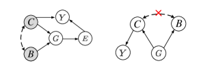
(a) DAG $\mathcal{G}$

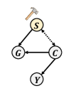
(b) DAG $\mathcal{H}$

Figure 1. two causal models driven from (Fan et al., 2022; Wu et al., 2021)

Recently, some studies (Feng et al., 2021; Fan et al., 2022; Wu et al., 2021) have conducted direct analysis on the causal relationships between deep representations. Drawing inspiration from domain generalization, these works divide deep representations into two distinct patterns: causal patterns and shortcut patterns. The causality graph constructed by this approach is as shown in Figure 1.

Within their approach, intervention is defined similarly to the creation of negative samples in self-supervised methods. The intervention is achieved by swapping the causal patterns and shortcut patterns of different samples, with the aim of predicting the correct causal pattern:

(24) $$\min\mathcal{R}_{DIR}=\mathbb{E}_{s}[\mathcal{R}(h(G),Y|do(S=s))]+\lambda Var_{s}(\{\mathcal{R}(h(G),Y|do(S=s))\})$$

6. The Challenges and Roadmaps of Indefinite Data Paradigms

Despite the challenges posed by the combination of multiple structures and multi-value variables, we aim to explore the two perspectives of both multiple structures and multi-valued variables, separately. In other words, when discussing the issues arising from multiple structures, it is assumed that multi-value data leads to the existence of $p:\mathcal{S}\rightarrow\mathcal{X}$. $q:\mathcal{X}\rightarrow\mathcal{\hat{X}}$ and similarly, multi-value data assumes that variable $f$ cannot be solved through statistical strength.

6.1. Multi-structure Perspectives

As mentioned in Section 3, the issue of multiple structures in the indefinite data paradigm has surpassed the fundamental challenges of clustering ability of samples and the dynamic capability to learn from different structures. Due to the disturbance caused by quantification inaccuracies, the learning ability of multi-structure models cannot be independent of the robustness and accuracy of deep learning. However, the success of deep learning techniques is primarily attributed to large-scale $i.i.d.$ datasets, which endow them with exceptional generalization capabilities on the same distribution (i.e., from one datapoint to another). However, their generalization abilities lag significantly on different distributions (i.e., from one dataset to another).

The relevant studies in Paper (Chen et al., 2023d) elucidated this situation by evaluating the performance of various methods for emotion inference in dialogues. These methods include task-specific supervised approaches and unsupervised approaches primarily based on large language models (LLMs) and pre-trained models. Table 4 presents the specific results, involving two specifically designed causal relation testing experiments:

Table 4. two challenges of causation examination (Chen et al., 2023d)

Methods	Challenge 1		Challenge 2
	($U_{a}$,$U_{b}$)	($U_{b}$,$U_{a}$)	($U_{a}$,$U_{b}$)	($U_{b}$,$U_{c}$)	($U_{a}$,$U_{c}$)
GPT-3.5 (Radford et al., 2019)	112	102	108	114	109
GPT-4 (OpenAI, 2023)	127	114	111	105	103
RoBERTa (Liu et al., 2019b)	95	97	94	91	83
RoBERTa+ (Liu et al., 2019b)	97	91	105	101	106
RANK-CP (Wei et al., 2020)	142	125	147	129	131
ECPE-2D (Ding et al., 2020)	151	153	142	138	146
EGAT (Chen et al., 2023b)	166	154	157	139	148

• Negative samples that involve interchanging outcome utterances and cause utterances. For such negative samples, the ability of deep models to recognize the Markovian causal relationships of $X_{i}\rightarrow X_{j}$ and $X_{j}\rightarrow X_{i}$ can be examined.

• Negative samples with intermediate variables. For such negative samples, the ability of the models to recognize the causal relationships of $X_{i}\rightarrow X_{j}$ and $X_{i}\rightarrow X_{k}\rightarrow X_{j}$ can be examined.

However, all the models did not exhibit significant causality discrimination in these two tests. Specifically, irrespective of positive or negative samples, the models learned similar associations. As mentioned in Section 2, existing deep model methods can only learn the existence of associations between two variables but are unable to discern the specific direction, such as $X_{i}\rightarrow X_{j}$ and $X_{j}\rightarrow X_{i}$. This lack of causality discrimination is a noteworthy limitation.

Table 5. Overall performance of CORR2CAUSE (Jin et al., 2023)

	F1	Precision	Recall	Accuracy
Random Baselines
Always Majority	0.0	0.0	0.0	84.77
Random (Proportional)	13.5	12.53	14.62	71.46
Random (Uniform)	20.38	15.11	31.29	62.78
BERT-Based Models
BERT MNLI (Devlin et al., 2019)	2.82	7.23	1.75	81.61
RoBERTa MNLI (Liu et al., 2019b)	22.79	34.73	16.96	82.50
DeBERTa MNLI (He et al., 2020)	14.52	14.71	14.33	74.31
DistilBERT MNLI (Sanh et al., 2019)	20.70	24.12	18.13	78.85
DistilBAET MNLI (Shleifer and Rush, 2020)	26.74	15.92	83.63	30.23
BART MNLI (Lewis et al., 2019)	33.38	31.59	35.38	78.50
LLaMa-Based Models
LLaMa-6.7B (Touvron et al., 2023)	26.81	15.50	99.42	17.36
Alpaca-6.7B(Taori et al., 2023)	27.37	15.93	97.37	21.33
GPT-Based Models
GPT-3 Ada (Brown et al., 2020)	0.00	0.00	0.00	84.77
GPT-3 Babbage (Brown et al., 2020)	27.45	15.96	97.95	21.15
GPT-3 Curie (Brown et al., 2020)	26.43	15.23	100.00	15.23
GPT-3 Davinci (Brown et al., 2020)	27.82	16.57	86.55	31.61
GPT-3 Instruct (text-davinci-001) (Ouyang et al., 2022)	17.99	11.84	37.43	48.04
GPT-3 Instruct (text-davinci-002) (Ouyang et al., 2022)	21.87	13.46	58.19	36.69
GPT-3 Instruct (text-davinci-003) (Ouyang et al., 2022)	15.72	13.4	19.01	68.97
GPT-3.5 (Radford et al., 2019)	21.69	17.79	27.78	69.46
GPT-4 (OpenAI, 2023)	29.08	20.92	47.66	64.60

Coincidentally, Paper (Jin et al., 2023) introduces a dataset called CORR2CAUSE, which is designed to assess the causal discrimination ability of LLMs. The dataset focuses on when causal inferences can be made based on correlation and when they cannot. Table 5 presents a more comprehensive evaluation of LLMs’ causality discrimination capability, further affirming that pure causal reasoning remains a highly challenging task for all current LLMs.

Fortunately, SCMs provide evidence for analyzing more precise causal relationships in the case of fitting two similar variables. Under the assumption of causal sufficiency, the common cause theorem implies that the noise terms must be independent. This independence introduces a discrepancy between the dependencies of $P(X_{i}|pa_{i})$ and $P(X_{j}|Pa_{j})$ with respect to the correlation between $X_{i}$ and $X_{j}$ (note that the independence of $U_{i}$ cannot be directly translated into the independence of $X_{i}$). In other words, when fitting $X_{i}$ and $X_{j}$, in addition to capturing their correlation, it becomes possible to uncover the causal relationship between $X_{i}$ and $X_{j}$. Following the setup in Paper (Chen et al., 2023d), let’s assume $\Sigma$ represents the residual after fitting variables $X_{i}$ and $X_{j}$. In this case, the conditional independence between the residual term and the variables is given by:

Definition 6.1 (Independent Conditions for causations from correlations).

The relationship of two utterances $X_{i}$ and $X_{j}$ in a dialogue is causal discriminable, from the independent conditions:

• $\Sigma_{X_{i}}\perp\!\!\!\perp X_{j},\Sigma_{X_{j}}\not\!\perp\!\!\!\perp X_{i}\Rightarrow X_{j}\rightarrow X_{i}$

• $\Sigma_{X_{i}}\not\!\perp\!\!\!\perp X_{j},\Sigma_{X_{j}}\perp\!\!\!\perp X_{i}\Rightarrow X_{i}\rightarrow X_{j}$

• $\Sigma_{X_{i}}\not\!\perp\!\!\!\perp X_{j},\Sigma_{X_{j}}\not\!\perp\!\!\!\perp X_{i}\Rightarrow L\rightarrow X_{i},L\rightarrow X_{j}$

• $\Sigma_{X_{i}}\perp\!\!\!\perp X_{j},\Sigma_{X_{j}}\perp\!\!\!\perp X_{i}\Rightarrow X_{i}\rightarrow L,X_{j}\rightarrow L$

Definition 6.1 indicates that for any two variables that can be fitted, incorporating independent noise terms allows for the inclusion of knowledge from correlation to causation. Therefore, the focus of causal discrimination lies in how to incorporate the noise terms. Paper (Chen et al., 2023c) summarizes the application of variational inference in previous causal discovery. Specifically, treating the noise terms as latent variables $Z$ and computing the reconstruction loss of causal representation has emerged as a popular framework. The log-evidence of this framework is expressed as:

(25) $$\frac{1}{N}\sum_{n=1}^{N}\log p(X_{n})=\frac{1}{N}\sum_{n=1}^{N}\log\int p(X_{n}|E)p(E)dE$$

6.2. Multi-value Perspectives

The issues arising from multi-value data in the indefinite data paradigm still revolve around quantification inaccuracies and statistical feature deviations. However, considering the impact of multiple structures, we concretize the problems into two aspects: 1) How to calculate the influence of latent confounders in the context of an unfixed causal model? 2) How to ensure the causal consistency between the causal representation and the causal model?

For 1), numerous studies (Miao et al., 2018; Zhu et al., 2022; Kallus et al., 2019; Shimizu and Bollen, 2014) have proposed approaches to handle confounders when it is not possible to make simplifying assumptions on the causal model. Instead of pinpointing the confounders, these approaches focus on disentangling the unattributed portion of the observed variables. Such methods represent $X$ as $\hat{X}+C$, where $C$ is represented in the form of a SCM:

(26) $$c_{m,j}=\sum_{l_{m,k}\in Ec(x_{m,j})}g_{m,kj}l_{m,k}(c\in\mathbb{R}^{N\times D},l\in\mathbb{R}^{K\times D},0\leq i\neq j,k<N)$$

According to the setting of SCMs, the observed target $X_{i}$ consists of an endogenous term ($f_{i}Pa_{i}$) and two exogenous terms ($g_{i}l_{m}andU_{i}$). Its causal model can be decoupled into two subgraphs, representing the pure relationships between $X$ variables ($f_{i}Pa_{i}+U_{i}$) and the remaining exogenous term coefficients ($g_{i}l_{m}$), as shown in Figure 2.  (Chen et al., 2023c) analyzed the distributions of the causal model under different states: complete state, confounding-free state, pure relationship state among $X$ variables, and confounding effect state. In the case of single-value data, the confounding impact can be assumed to follow the distribution $P(X|L)$. However, this advantage does not hold for multi-value data. Hence,  (Chen et al., 2023c) further proposes an approximate estimation for the confounding effect.

Definition 6.2.

there exist an approximate estimation

(27) $$C_{j}=\frac{\mathbb{P}(x_{j})\mathbb{P}(L|x_{j})}{\sum_{i}^{N}\mathbb{P}(x_{i})\mathbb{P}(L|x_{i})}x_{j}$$

when the latent variables $l$ vastly outweigh independent noise $\epsilon_{x}$.

(a) DAG $\mathcal{G}$

(b) DAG $\mathcal{H}$

(c) DAG $\mathcal{O}$

(d) DAG $\mathcal{C}$

Figure 2. Four causal DAGs discussed in (Chen et al., 2023c).

Regarding 2), we have addressed this issue in Section 3. Specifically, assuming the parameters of the encoder as $\varphi$ and the parameters of the decoder as $\theta$, we can infer that in the context of indefinite data paradigms, the causal model can be expressed as $\mathcal{G}=F(X,\varphi)$, while for causal representation, it can be written as $Y=H(X,a,b)$. This leads to the indefinite data paradigm being the only data type where inconsistencies between the causal model and causal representation may exist (in single-structure models, the causal model $\mathcal{G}$ is fixed, and in single-value variables, $\varphi$ and $\theta$ do not exist). Furthermore, considering that most existing encoder-decoder structures  (Rezende and Mohamed, 2015; Wijmans and Baker, 1995; Zhang et al., 2018; Creswell et al., 2018) lack constraints on $\theta$ w.r.t. $\varphi$ (i.e., $\theta=\omega(\varphi)$), the causal representation and causal model generated by the indefinite data paradigm often exhibit inconsistencies, resulting in less intelligent behavior when it comes to out-of-distribution generalization.

Intervention (i.e., $do$ operator) is a well-recognized approach for testing causal consistency, but it is ineffective under the indefinite data paradigm when it comes to computing adjustment $Z$ formulas or controlling variable distributions. However, in essence, the indefinite data can achieve consistency with intervention by constraining the inputs of deep models to control the set of parent nodes involved in the computation, thus ensuring that the parent node set of the target variable $X$ is an empty set. Additionally, for the problem of consistency between two causal models, works such as exact transformation and causal abstraction provide a theoretical basis based on the intervention set  (Rubenstein et al., 2017; Geiger et al., 2021; Beckers and Halpern, 2019).

7. Datasets from Three Data Paradigms

7.1. Datasets for Definite Data

The definite datasets are characterized by single-value and single-structure features, often manifested in the form of structured data. Each variable consists of single valued attributes, such as body temperature, age, wind strength, economic growth rate, population count, protein quantity, and more. Furthermore, all the data points are obtained from sampling conducted under the same $i.i.d.$ environment, suggesting that all samples mirror the same causal model. Table 6 lists numerous popular definite datasets along with brief summaries of their characteristics.

Table 6. Definite Datasets

Datasets	$\#variables$	Highlights
Erdos-Rényi Graphs	Customization	Number of probabilities based on custom nodes $p=\frac{2e}{d^{2}}$ adding edges
Twins (Almond et al., 2005)	Customization	twin births in the United States between 1989-1991
SynTReN (Van den Bulcke et al., 2006)	Customization	Synthetic gene expression data
Census Income KDD (Ristanoski et al., 2013)	3	The Census Income (KDD) data set (US)
ADNI (Jack Jr et al., 2008)	3	three latent representation outputs about Alzheimer’s Disease
CPRD (Herrett et al., 2015)	4	medical records from NHS general practice clinics in the UK
Economic data (Iacoviello and Navarro, 2019)	4	Quarterly data for the United States 1965 - 2017
Arrhythmia (Asuncion and Newman, 2007)	4	from the UCI Machine Learning Repository concerns cardiac arrhythmia
DWD climate (Dietrich et al., 2019)	6	Data from 349 weather stations in Germany
IHDP (Brooks-Gunn et al., 1992)	8	originated from preterm infants with low birth weight
Archaeology (Huang et al., 2018)	8	Archaeological data
Soil Properties (Solly et al., 2014)	8	Biological root decomposition data
AutoMPG (Asuncion and Newman, 2007)	9	Fuel consumption data for city car cycles
Abalone (Nash et al., 1994)	9	Conch abalone size data
HK Stock Market (Huang et al., 2020)	10	Dividend-adjusted daily closing prices of 10 major stocks
Sachs (Sachs et al., 2005)	11	Proteins and phospholipids in human cells
Breast Cancer Wisconsim (Asuncion and Newman, 2007)	11	Breast cancer cell data
TCGA (Weinstein et al., 2013)	12	a comprehensive and extensive database of genomic information
CHESS (Qian et al., 2020)	14	ICU patients during the first wave of the COVID-19
CogUSA study (Tu et al., 2019)	16	Cognitive ageing data
Jobs (LaLonde, 1986)	16	assess the effect of vocational training on employment outcomes
fMRI (Wang et al., 2003)	25	The different voxel data in fMRI were organised into ROIs

The definite datasets mainly originates from various real-world domains, with the most frequently represented being the fields of medicine and disease  (Almond et al., 2005; Van den Bulcke et al., 2006; Herrett et al., 2015; Jack Jr et al., 2008; Asuncion and Newman, 2007; Sachs et al., 2005; Asuncion and Newman, 2007; Weinstein et al., 2013; Tu et al., 2019; Wang et al., 2003; Qian et al., 2020), followed by finance  (Ristanoski et al., 2013; Iacoviello and Navarro, 2019; Asuncion and Newman, 2007; Huang et al., 2020; LaLonde, 1986) and nature  (Dietrich et al., 2019; Brooks-Gunn et al., 1992; Huang et al., 2018; Solly et al., 2014; Nash et al., 1994). Such datasets typically exhibit two characteristics: 1) a small number of observed variables, and 2) a large sample size. When combined with the attributes of single-structure and single-value data, these datasets often facilitate the identification of quite accurate causal structures. Furthermore, they reveal the real-world meanings of these causal relations.

A further consideration arises from realities of data collection, where errors and issues can result in incomplete data. This situation has fueled the emergence of causal completion tasks that aim at imputing missing values based on the observed causal associations. Another phenomenon borne out by the limited number of observed variables accounting for the whole system is the confounding bias problem. It has thus prompted corresponding research on confounding factors.

With these datasets, researchers hardly need to worry about the structure of the causal relationship. A fully connected undirected graph, built upon the provided observed variables of the dataset, can serve to establish a complete causal structure. The primary focus of the statistical study then becomes how to utilize this data to derive the causal relation between pairs of variables. That is, determining which undirected edges should be retained and subsequently directed. This process embodies the cores of their domain-specific research.

7.2. Datasets for Semi-definite Data

Semi-definite datasets can be broadly categorized into two types: multi-structure $\&$ single-value data, and single-structure $\&$ multi-value data. The former type essentially only includes temporal datasets such as financial time series or blood oxygen level time series. Meanwhile, the latter type traverses a majority of disparate modalities including but not limited to image datasets and text datasets. To provide a grip on these diverse dataset types, we have articulated their respective examples and highlights in Table 7.

Table 7. Semi-Definite Datasets

Datasets	Types	Highlights
CMU MoCap (CMUMoCap, 2008)	time series	containing data about joint angles, body position
DREAM-3 (Prill et al., 2010)	time series	continuous gene expression and regulation dynamics
BOLD (BOLD, 2012)	time series	different brain regions of interest in human subjects
MemeTracker (MemeTracker, 2018)	time series	online articles’ website, publication time, and all the hyperlinks
IPTV (Luo et al., 2014)	time series	the user’s viewing behavior, i.e., what program and when they watch in the IPTV systems
G-7 (Demirer et al., 2018)	time series	daily return volatility of sovereign bonds of countries in the Group of Seven
CIFAR-10/100 (Krizhevsky et al., 2009)	image	each respectively containing fine-grained and coarse-grained labels representing the image.
ImageNet (Deng et al., 2009)	image	More than 20,000 categories of image recognition data
ObjectNet (Barbu et al., 2019)	iamge	objects are shown in different camera angles in a cluttered room
YFCC-100M Flickr (Karkkainen and Joo, 2021)	image	Facial recognition data
Casual Conversations (Hazirbas et al., 2021)	image	Facial recognition dataset that can include age, gender, and skin color as classification tags.
CUB200-2011 (Wah et al., 2011)	image	Includes identification data for 200 different bird species.
Aff-wild2 (Kollias and Zafeiriou, 2018)	image	a wide variation of subjects in terms of posture, age, lighting conditions, race and occupation
Market1501 (Zheng et al., 2015)	image	Pedestrian re-identification dataset
Cityscapes (Hu et al., 2020)	image	Street scene recognition data from 50 different cities.
Amazon reviews (Mudambi and Schuff, 2010)	text	Amazon.com product reviews related to books, electronics, clothing and other 26 categories
OntoNotes$5$ (Dror et al., 2017)	text	Large news corpus, including 7 types
CFPB compliant (Tan et al., 2022)	text	U.S. Consumer Financial Protection Bureau (CFPB) Consumer Complaint Data
SNIPS (Larson et al., 2019)	text	The personal voice assistant collects data containing 7 domains
CrisistextLine (Gould et al., 2022)	text	Session data of counselor and mentee
Yelp (Luca, 2016)	text	Merchant review site user review data in Yelp
CNC (Tan et al., 2022)	text	Social News Data Corpus
AG’news (Zhang et al., 2015b)	text	Classified coverage from over 2,000 news sources
Gender Citation Gap (Maliniak et al., 2013)	text	Data from the TRIP database obtained from the IR literature
Weiboscope (Fu et al., 2013)	text	Real-time posting data of Weibo social media users
JDDC (Chen et al., 2019)	text	D customer service staff on the topic of after-sales conversations
Spurious-Motif (Ying et al., 2019)	graph	Each graph is composed of one base and one motif
MNIST-75sp (Knyazev et al., 2019)	graph	converts the MNIST images into 70000 superpixel graphs with at most 75 nodes each graph
Graph-SST2 (Socher et al., 2013)	graph	Each graph is labeled by its sentence sentiment
Molhiv (Wu et al., 2018)	graph	nodes are atoms, and edges are chemical bonds
BA-Shapes (Barabási and Albert, 1999)	graph	80 five-node motifs are randomly attached to the base graph
MUTAG (Debnath et al., 1991)	graph	Every graph is labeled according to their mutagenic effect on the bacterium
OGBG-Mol (Wu et al., 2018)	graph	Graphs represent molecules and labels are chemical properties of molecules

Compared to defined datasets, semi-definite datasets span a more diverse range of areas, primarily due to the expansion from single-value data to multi-value data. This shift has enabled image, text, and graph data to be incorporated into causal discovery, and the development of multi-structure datasets introduces the novel data type of time series. For instance, ImageNet and Cifar-10 image datasets were not initially intended for causal discovery. However, with the convergence of causal discovery and deep learning, explaining the classification and identification of an entire image based on the semantics of its components has become a popular choice. The same pattern can be found in text datasets. For example, the CFPB compliant dataset contains records of consumer complaints and whether they were resolved timely, which can be used to build semi-definite causal models to identify the features of complaints that can be resolved. Graph datasets are most invloved with interpretability of GNN via analysing the causal relationships between shortcuts and causal features. Consequently, we did not list the number of causal variables, as depending on the high-level task, causal variables could represent a subset or a mapping of the observed variables. Similarly, we did not tackle the the number of causal structures in time-series datasets, as the number of structures is indeterminate depending on the causal variables involved.

7.3. Datasets for Indefinite Data

Indefinite datasets contain multi-structure samples, and every sample incorporates multi-value variables. From a machine learning data resource perspective, indefinite datasets possess characteristics of both types of semi-definite datasets. In other words, they are more likely to be temporal multi-value datasets, such as dialog and video datasets.

However, it’s important to note that temporality is not a defined property of indefinite datasets. The association exists largely because, in the real world, most multi-structure data naturally occur as temporal sequences. Their variable lengths and partial non-replicability contribute to the multi-structure data type. But it should be stressed that multi-structure does not inherently imply temporality. (While this kind of raw data is challenging to collect in the real world, we can imagine its existence. For example, by disrupting and randomly reordering the sequence of interactions within a dialog dataset, the resulting dataset loses its temporal quality.) The same notion is also applicable to multi-structure datasets within the semi-definite data.

When viewed from a causal discovery perspective, indefinite datasets share significant intersections with semi-definite datasets. Many datasets, while originally developed for semi-definite tasks, could transition to indefinite datasets by relaxing the constraints on structure or values. However, these indefinite tasks are often ill-posed, requiring additional prior knowledge or assumptions for their resolution.

Table 8. Datasets which can be regarded as indefinite datasets

Datasets	Types	Original tasks	Highlights
DailyDialog (Li et al., 2017)	text	ER,AR,ECG	A daily conversation dataset annotated with 7 emotions, 4 actions and 10 themes
CORR2CAUSE (Jin et al., 2023)	text	CI,CoT	A text datasets for large language model with causal labels
MultiArith (Roy and Roth, 2016)	text	QA,AR,CoT	an arithmetic datasets with multiple steps and operations
CSQA (Talmor et al., 2018)	text	QA,CR,CoT	A commonsense datasets answering with piror knowledge
Coin Flip (Wei et al., 2022)	text	QA,SR,CoT	A symbolic reasoning datasets which can be used in large language model
CAER (Lee et al., 2019)	video	ER,CI	a drama video datasets with 7 emotion labels
50salads (Stein and McKenna, 2013)	video	AR,CI	a video datasets composed of action parts with 17 action labels
Bach Chorales dataset (Román et al., 2019)	audio	MG,PG	Bach’s four-part congregational hymn dataset
MedleyDB (Bittner et al., 2014)	audio	MG,PG	Polyphonic Pop Music Dataset
IEMOCAP (Busso et al., 2008)	multimodal	ERC,NLU,CI	A conversation script for 10 male and female actors with emotion labels

Table 8 showcases a collection of potential indefinite datasets we’ve compiled. While these datasets involve diverse modalities and tasks, under certain conditions, they all fulfill the characteristics of multi-structure and multi-value variables, with causal relations between variables being particularly significant. For instance, in the DailyDialog dataset, some studies have annotated the causes of emotions (Poria et al., 2021; Chen et al., 2023d), leading to the recognition of spans of causes. In this type of task, each dialog represents a unique causal structure, whereas each utterance acts as a multi-value variable. The 50salads dataset, meanwhile, investigates task segmentation in videos via automated action recognition. Each video is treated as a distinct causal model with various segments acting as multi-value variables. Understanding the relations between these segments through causal relationships among the multi-value variables is a crucial point of this task. Datasets associated with the CoT task explore the causal relationships between each step. Audio modality datasets also focus on the mutual influences between different polyphonic vioces.

8. Conclusion

In this paper, we redefine existing causal data from two perspectives, causal structure and causal representation, to allow it to be embedded appropriately within the theories and methods of deep learning, forming an throughout and comprehensive domain.

Firstly, we redefine fundamental concepts such as causal model, causal variable, and causal representation, introducing the differences in existing data regarding structure and representation. Specifically, we use the term “multi-structure data” to denote cases where the causal structure is not unique, and “single-structure data” for those with a fixed causal structure. We employ “multi-value variables” to refer to data that requires deep representation for computations in causal variables, and “single-value variables” to encompass statistical data that exists in numerical form without the need for deep representation. Based on structural and representational differences, we define three different data paradigms: definite data (single-structure and single-value), semi-definite data (single-structure and multi-value, or multi-structure and single-value), and indefinite data (multi-structure and multi-value). We exemplify their differences by their forms, analyze the distinct problems they face in terms of resolution pathways, and summarize their respective development directions in the evolution of researches.

Definite and semi-definite data, as mature research domains, have been discussed in relation to various tasks to highlight their current application scenarios. Definite data primarily involves causal discovery, causal discovery with latent confounders, and causal effect estimation. Semi-definite data mainly concerns causal data related to time series, images, text, other modalities, and deep representations. However, indefinite data is still in its infancy. We consider structure and representation to envision roadmaps for situations dealing with simultaneous multi-structure and multi-value data based on existing research problems.

Lastly, we organize datasets commonly used in the three data paradigms, briefly introduce their attributes, and summarize their application fields.

The three data paradigms proposed encompass nearly all causal models, especially upon including unstructured inputs such as images and texts. We hope these three data paradigms can provide readers with broader causal insights. When confronted with specific causal data, they can follow the categorization in this review to capture the key features and challenges of the data type, thereby identifying the baselines of deep models and causal theories.

References

- (1)
- Agrawal et al. (2021) Raj Agrawal, Chandler Squires, Neha Prasad, and Caroline Uhler. 2021. The DeCAMFounder: Non-linear causal discovery in the presence of hidden variables. arXiv preprint arXiv:2102.07921 (2021).
- Ahuja et al. (2022) Kartik Ahuja, Jason S Hartford, and Yoshua Bengio. 2022. Weakly supervised representation learning with sparse perturbations. Advances in Neural Information Processing Systems 35 (2022), 15516–15528.
- Akbari et al. (2021) Sina Akbari, Ehsan Mokhtarian, AmirEmad Ghassami, and Negar Kiyavash. 2021. Recursive causal structure learning in the presence of latent variables and selection bias. Advances in Neural Information Processing Systems 34 (2021), 10119–10130.
- Alaa et al. (2017) Ahmed M Alaa, Michael Weisz, and Mihaela Van Der Schaar. 2017. Deep counterfactual networks with propensity-dropout. arXiv preprint arXiv:1706.05966 (2017).
- Almond et al. (2005) Douglas Almond, Kenneth Y Chay, and David S Lee. 2005. The costs of low birth weight. The Quarterly Journal of Economics 120, 3 (2005), 1031–1083.
- Anandkumar et al. (2013) Animashree Anandkumar, Daniel Hsu, Adel Javanmard, and Sham Kakade. 2013. Learning linear bayesian networks with latent variables. In International Conference on Machine Learning. PMLR, 249–257.
- Anciukevicius et al. (2022) Titas Anciukevicius, Patrick Fox-Roberts, Edward Rosten, and Paul Henderson. 2022. Unsupervised Causal Generative Understanding of Images. Advances in Neural Information Processing Systems 35 (2022), 37037–37054.
- Ancona et al. (2004) Nicola Ancona, Daniele Marinazzo, and Sebastiano Stramaglia. 2004. Radial basis function approach to nonlinear Granger causality of time series. Physical Review E 70, 5 (2004), 056221.
- Assaad et al. (2022) Charles K Assaad, Emilie Devijver, and Eric Gaussier. 2022. Survey and evaluation of causal discovery methods for time series. Journal of Artificial Intelligence Research 73 (2022), 767–819.
- Asuncion and Newman (2007) Arthur Asuncion and David Newman. 2007. UCI machine learning repository.
- Athey and Imbens (2016) Susan Athey and Guido Imbens. 2016. Recursive partitioning for heterogeneous causal effects. Proceedings of the National Academy of Sciences 113, 27 (2016), 7353–7360.
- Athey and Imbens (2015) Susan Athey and Guido W Imbens. 2015. Machine learning methods for estimating heterogeneous causal effects. stat 1050, 5 (2015), 1–26.
- Badura et al. (2018) Petr Badura, Andrea Madarasova Geckova, Dagmar Sigmundova, Erik Sigmund, Jitse P van Dijk, and Sijmen A Reijneveld. 2018. Can organized leisure-time activities buffer the negative outcomes of unstructured activities for adolescents’ health? International journal of public health 63 (2018), 743–751.
- Balashankar and Subramanian (2021) Ananth Balashankar and Lakshminarayanan Subramanian. 2021. Learning faithful representations of causal graphs. In Proceedings of the 59th Annual Meeting of the Association for Computational Linguistics and the 11th International Joint Conference on Natural Language Processing (Volume 1: Long Papers). 839–850.
- Barabási and Albert (1999) Albert-László Barabási and Réka Albert. 1999. Emergence of scaling in random networks. science 286, 5439 (1999), 509–512.
- Barbu et al. (2019) Andrei Barbu, David Mayo, Julian Alverio, William Luo, Christopher Wang, Dan Gutfreund, Josh Tenenbaum, and Boris Katz. 2019. Objectnet: A large-scale bias-controlled dataset for pushing the limits of object recognition models. Advances in neural information processing systems 32 (2019).
- Beamer et al. (2008) Brandon Beamer, Alla Rozovskaya, and Roxana Girju. 2008. Automatic Semantic Relation Extraction with Multiple Boundary Generation.. In AAAI. 824–829.
- Beckers and Halpern (2019) Sander Beckers and Joseph Y Halpern. 2019. Abstracting causal models. In Proceedings of the aaai conference on artificial intelligence, Vol. 33. 2678–2685.
- Belloni et al. (2017) Alexandre Belloni, Victor Chernozhukov, Iván Fernández-Val, and Christian Hansen. 2017. Program evaluation and causal inference with high-dimensional data. Econometrica 85, 1 (2017), 233–298.
- Beltagy et al. (2019) Iz Beltagy, Kyle Lo, and Arman Cohan. 2019. SciBERT: A pretrained language model for scientific text. arXiv preprint arXiv:1903.10676 (2019).
- Bernstein et al. (2020) Daniel Bernstein, Basil Saeed, Chandler Squires, and Caroline Uhler. 2020. Ordering-based causal structure learning in the presence of latent variables. In International Conference on Artificial Intelligence and Statistics. PMLR, 4098–4108.
- Bhattacharya et al. (2021) Rohit Bhattacharya, Tushar Nagarajan, Daniel Malinsky, and Ilya Shpitser. 2021. Differentiable causal discovery under unmeasured confounding. In International Conference on Artificial Intelligence and Statistics. PMLR, 2314–2322.
- Bittner et al. (2014) Rachel M Bittner, Justin Salamon, Mike Tierney, Matthias Mauch, Chris Cannam, and Juan Pablo Bello. 2014. Medleydb: A multitrack dataset for annotation-intensive mir research.. In ISMIR, Vol. 14. 155–160.
- BOLD (2012) BOLD 2012. NetSim - Evaluation of Network Modelling Methods for FMRI. https://www.fmrib.ox.ac.uk/datasets/netsim/index.html.
- Brooks-Gunn et al. (1992) Jeanne Brooks-Gunn, Fong-ruey Liaw, and Pamela Kato Klebanov. 1992. Effects of early intervention on cognitive function of low birth weight preterm infants. The Journal of pediatrics 120, 3 (1992), 350–359.
- Brown et al. (2020) Tom Brown, Benjamin Mann, Nick Ryder, Melanie Subbiah, Jared D Kaplan, Prafulla Dhariwal, Arvind Neelakantan, Pranav Shyam, Girish Sastry, Amanda Askell, et al. 2020. Language models are few-shot learners. Advances in neural information processing systems 33 (2020), 1877–1901.
- Busso et al. (2008) Carlos Busso, Murtaza Bulut, Chi-Chun Lee, Abe Kazemzadeh, Emily Mower, Samuel Kim, Jeannette N Chang, Sungbok Lee, and Shrikanth S Narayanan. 2008. IEMOCAP: Interactive emotional dyadic motion capture database. Language resources and evaluation 42, 4 (2008), 335–359.
- Cai et al. (2019) Ruichu Cai, Feng Xie, Clark Glymour, Zhifeng Hao, and Kun Zhang. 2019. Triad constraints for learning causal structure of latent variables. Advances in neural information processing systems 32 (2019).
- Cai et al. (2020) Ruichu Cai, Jincheng Ye, Jie Qiao, Huiyuan Fu, and Zhifeng Hao. 2020. FOM: Fourth-order moment based causal direction identification on the heteroscedastic data. Neural Networks 124 (2020), 193–201.
- Chakraborty and Murphy (2014) Bibhas Chakraborty and Susan A Murphy. 2014. Dynamic treatment regimes. Annual review of statistics and its application 1 (2014), 447–464.
- Chalupka et al. (2017) Krzysztof Chalupka, Frederick Eberhardt, and Pietro Perona. 2017. Causal feature learning: an overview. Behaviormetrika 44 (2017), 137–164.
- Chang and Dy (2017) Yale Chang and Jennifer Dy. 2017. Informative subspace learning for counterfactual inference. In Proceedings of the AAAI Conference on Artificial Intelligence, Vol. 31.
- Chen et al. (2023a) Hang Chen, Bingyu Liao, Jing Luo, Wenjing Zhu, and Xinyu Yang. 2023a. Learning a Structural Causal Model for Intuition Reasoning in Conversation. arXiv:2305.17727 [cs.CL]
- Chen et al. (2023b) Hang Chen, Xinyu Yang, and Chenguang Li. 2023b. Learning a General Clause-to-Clause Relationships for Enhancing Emotion-Cause Pair Extraction. arXiv:2208.13549 [cs.CL]
- Chen et al. (2023d) Hang Chen, Xinyu Yang, Jing Luo, and Wenjing Zhu. 2023d. How to Enhance Causal Discrimination of Utterances: A Case on Affective Reasoning. Proceedings of the 2023 Conference on Empirical Methods in Natural Language Processing (EMNLP)” (2023).
- Chen et al. (2023c) Hang Chen, Xinyu Yang, and Qing Yang. 2023c. Learning to Recover Causal Relationship from Indefinite Data in the Presence of Latent Confounders. arXiv preprint arXiv:2305.02640 (2023).
- Chen et al. (2016) Jifan Chen, Qi Zhang, Pengfei Liu, Xipeng Qiu, and Xuan-Jing Huang. 2016. Implicit discourse relation detection via a deep architecture with gated relevance network. In Proceedings of the 54th Annual Meeting of the Association for Computational Linguistics (Volume 1: Long Papers). 1726–1735.
- Chen et al. (2019) Meng Chen, Ruixue Liu, Lei Shen, Shaozu Yuan, Jingyan Zhou, Youzheng Wu, Xiaodong He, and Bowen Zhou. 2019. The jddc corpus: A large-scale multi-turn chinese dialogue dataset for e-commerce customer service. arXiv preprint arXiv:1911.09969 (2019).
- Chen and Chan (2013) Zhitang Chen and Laiwan Chan. 2013. Causality in linear nongaussian acyclic models in the presence of latent gaussian confounders. Neural Computation 25, 6 (2013), 1605–1641.
- Chicco and Jurman (2020) Davide Chicco and Giuseppe Jurman. 2020. The advantages of the Matthews correlation coefficient (MCC) over F1 score and accuracy in binary classification evaluation. BMC genomics 21, 1 (2020), 1–13.
- Chickering (2002) David Maxwell Chickering. 2002. Optimal structure identification with greedy search. Journal of machine learning research 3, Nov (2002), 507–554.
- Chu et al. (2008) Tianjiao Chu, Clark Glymour, and Greg Ridgeway. 2008. Search for Additive Nonlinear Time Series Causal Models. Journal of Machine Learning Research 9, 5 (2008).
- Chu et al. (2020) Zhixuan Chu, Stephen L Rathbun, and Sheng Li. 2020. Matching in selective and balanced representation space for treatment effects estimation. In Proceedings of the 29th ACM International Conference on Information & Knowledge Management. 205–214.
- Claggett and Karahanna (2018) Jennifer L Claggett and Elena Karahanna. 2018. Unpacking the structure of coordination mechanisms and the role of relational coordination in an era of digitally mediated work processes. Academy of Management Review 43, 4 (2018), 704–722.
- Cleary and Witten (1984) J Cleary and I Witten. 1984. A comparison of enumerative and adaptive codes. IEEE Transactions on Information Theory 30, 2 (1984), 306–315.
- CMUMoCap (2008) CMUMoCap 2008. CMU Graphics Lab Motion Capture Database. http://mocap.cs.cmu.edu/.
- Colombo et al. (2012) Diego Colombo, Marloes H Maathuis, Markus Kalisch, and Thomas S Richardson. 2012. Learning high-dimensional directed acyclic graphs with latent and selection variables. The Annals of Statistics (2012), 294–321.
- Creswell et al. (2018) Antonia Creswell, Tom White, Vincent Dumoulin, Kai Arulkumaran, Biswa Sengupta, and Anil A Bharath. 2018. Generative adversarial networks: An overview. IEEE signal processing magazine 35, 1 (2018), 53–65.
- Dai et al. (1997) Honghua Dai, Kevin B Korb, Chris S Wallace, and Xindong Wu. 1997. A Study of Causal Discovery With Weak Links and Small Samples.. In IJCAI. Citeseer, 1304–1309.
- De Campos and Ji (2011) Cassio P De Campos and Qiang Ji. 2011. Efficient structure learning of Bayesian networks using constraints. The Journal of Machine Learning Research 12 (2011), 663–689.
- Debnath et al. (1991) Asim Kumar Debnath, Rosa L Lopez de Compadre, Gargi Debnath, Alan J Shusterman, and Corwin Hansch. 1991. Structure-activity relationship of mutagenic aromatic and heteroaromatic nitro compounds. correlation with molecular orbital energies and hydrophobicity. Journal of medicinal chemistry 34, 2 (1991), 786–797.
- Demirer et al. (2018) Mert Demirer, Francis X Diebold, Laura Liu, and Kamil Yilmaz. 2018. Estimating global bank network connectedness. Journal of Applied Econometrics 33, 1 (2018), 1–15.
- Deng et al. (2009) Jia Deng, Wei Dong, Richard Socher, Li-Jia Li, Kai Li, and Li Fei-Fei. 2009. Imagenet: A large-scale hierarchical image database. In 2009 IEEE conference on computer vision and pattern recognition. Ieee, 248–255.
- Deng et al. (2022) Zizhen Deng, Xiaolong Zheng, Hu Tian, and Daniel Dajun Zeng. 2022. Deep Causal Learning: Representation, Discovery and Inference. arXiv preprint arXiv:2211.03374 (2022).
- Devlin et al. (2019) Jacob Devlin, Ming-Wei Chang, Kenton Lee, and Kristina Toutanova. 2019. BERT: Pre-training of Deep Bidirectional Transformers for Language Understanding. arXiv:1810.04805 [cs.CL]
- Dietrich et al. (2019) Helge Dietrich, Thilo Wolf, Tobias Kawohl, Jan Wehberg, Gerald Kändler, Tobias Mette, Arno Röder, and Jürgen Böhner. 2019. Temporal and spatial high-resolution climate data from 1961 to 2100 for the German National Forest Inventory (NFI). Annals of Forest Science 76, 1 (2019), 1–14.
- Ding et al. (2020) Zixiang Ding, Rui Xia, and Jianfei Yu. 2020. ECPE-2D: Emotion-Cause Pair Extraction based on Joint Two-Dimensional Representation, Interaction and Prediction. In Proceedings of the 58th Annual Meeting of the Association for Computational Linguistics. Association for Computational Linguistics, Online, 3161–3170. https://doi.org/10.18653/v1/2020.acl-main.288
- Dittadi et al. (2020) Andrea Dittadi, Frederik Träuble, Francesco Locatello, Manuel Wüthrich, Vaibhav Agrawal, Ole Winther, Stefan Bauer, and Bernhard Schölkopf. 2020. On the transfer of disentangled representations in realistic settings. arXiv preprint arXiv:2010.14407 (2020).
- Dougherty et al. (1985) Thomas W Dougherty, Allen C Bluedorn, and Thomas L Keon. 1985. Precursors of employee turnover: A multiple-sample causal analysis. Journal of Organizational Behavior 6, 4 (1985), 259–271.
- Dror et al. (2017) Rotem Dror, Gili Baumer, Marina Bogomolov, and Roi Reichart. 2017. Replicability analysis for natural language processing: Testing significance with multiple datasets. Transactions of the Association for Computational Linguistics 5 (2017), 471–486.
- Entner and Hoyer (2010) Doris Entner and Patrik O Hoyer. 2010. On causal discovery from time series data using FCI. Probabilistic graphical models (2010), 121–128.
- Entner and Hoyer (2011) Doris Entner and Patrik O Hoyer. 2011. Discovering unconfounded causal relationships using linear non-gaussian models. In New Frontiers in Artificial Intelligence: JSAI-isAI 2010 Workshops, LENLS, JURISIN, AMBN, ISS, Tokyo, Japan, November 18-19, 2010, Revised Selected Papers 2. Springer, 181–195.
- Erdem et al. (2011) Esra Erdem, Kadir Haspalamutgil, Can Palaz, Volkan Patoglu, and Tansel Uras. 2011. Combining high-level causal reasoning with low-level geometric reasoning and motion planning for robotic manipulation. In 2011 IEEE International Conference on Robotics and Automation. 4575–4581. https://doi.org/10.1109/ICRA.2011.5980160
- Fan et al. (2022) Shaohua Fan, Xiao Wang, Yanhu Mo, Chuan Shi, and Jian Tang. 2022. Debiasing Graph Neural Networks via Learning Disentangled Causal Substructure. arXiv preprint arXiv:2209.14107 (2022).
- Feng et al. (2021) Qizhang Feng, Ninghao Liu, Fan Yang, Ruixiang Tang, Mengnan Du, and Xia Hu. 2021. DEGREE: Decomposition Based Explanation for Graph Neural Networks. In International Conference on Learning Representations.
- Fong et al. (2018) Christian Fong, Chad Hazlett, and Kosuke Imai. 2018. Covariate balancing propensity score for a continuous treatment: Application to the efficacy of political advertisements. The Annals of Applied Statistics 12, 1 (2018), 156–177.
- Frangakis and Rubin (2002) Constantine E Frangakis and Donald B Rubin. 2002. Principal stratification in causal inference. Biometrics 58, 1 (2002), 21–29.
- Friedman et al. (2013) Nir Friedman, Kevin Murphy, and Stuart Russell. 2013. Learning the structure of dynamic probabilistic networks. arXiv preprint arXiv:1301.7374 (2013).
- Fu et al. (2013) King-wa Fu, Chung-hong Chan, and Michael Chau. 2013. Assessing censorship on microblogs in China: Discriminatory keyword analysis and the real-name registration policy. IEEE internet computing 17, 3 (2013), 42–50.
- Gabler et al. (2023) Philipp Gabler, Bernhard C Geiger, Barbara Schuppler, and Roman Kern. 2023. Reconsidering Read and Spontaneous Speech: Causal Perspectives on the Generation of Training Data for Automatic Speech Recognition. Information 14, 2 (2023), 137.
- Galanti et al. (2020) Tomer Galanti, Ofir Nabati, and Lior Wolf. 2020. A critical view of the structural causal model. arXiv preprint arXiv:2002.10007 (2020).
- Gao et al. (2022) Chen Gao, Yu Zheng, Wenjie Wang, Fuli Feng, Xiangnan He, and Yong Li. 2022. Causal inference in recommender systems: A survey and future directions. arXiv preprint arXiv:2208.12397 (2022).
- Geiger et al. (2021) Atticus Geiger, Hanson Lu, Thomas Icard, and Christopher Potts. 2021. Causal abstractions of neural networks. Advances in Neural Information Processing Systems 34 (2021), 9574–9586.
- Geiger et al. (2023) Atticus Geiger, Zhengxuan Wu, Christopher Potts, Thomas Icard, and Noah D Goodman. 2023. Finding alignments between interpretable causal variables and distributed neural representations. arXiv preprint arXiv:2303.02536 (2023).
- Girju (2003) Roxana Girju. 2003. Automatic detection of causal relations for question answering. In Proceedings of the ACL 2003 workshop on Multilingual summarization and question answering. 76–83.
- Girju et al. (2009) Roxana Girju, Preslav Nakov, Vivi Nastase, Stan Szpakowicz, Peter Turney, and Deniz Yuret. 2009. Classification of semantic relations between nominals. Language Resources and Evaluation 43 (2009), 105–121.
- Glymour et al. (2019) Clark Glymour, Kun Zhang, and Peter Spirtes. 2019. Review of causal discovery methods based on graphical models. Frontiers in genetics 10 (2019), 524.
- Gong et al. (2023) Chang Gong, Di Yao, Chuzhe Zhang, Wenbin Li, and Jingping Bi. 2023. Causal Discovery from Temporal Data: An Overview and New Perspectives. arXiv preprint arXiv:2303.10112 (2023).
- Goudet et al. (2017) Olivier Goudet, Diviyan Kalainathan, Philippe Caillou, Isabelle Guyon, David Lopez-Paz, and Michèle Sebag. 2017. Causal generative neural networks. arXiv preprint arXiv:1711.08936 (2017).
- Goudet et al. (2018) Olivier Goudet, Diviyan Kalainathan, Philippe Caillou, Isabelle Guyon, David Lopez-Paz, and Michele Sebag. 2018. Learning functional causal models with generative neural networks. Explainable and interpretable models in computer vision and machine learning (2018), 39–80.
- Gould et al. (2022) Madelyn S Gould, Anthony Pisani, Carlos Gallo, Ashkan Ertefaie, Donald Harrington, Caroline Kelberman, and Shannon Green. 2022. Crisis text-line interventions: Evaluation of texters’ perceptions of effectiveness. Suicide and Life-Threatening Behavior (2022).
- Goyal et al. (2020) Anirudh Goyal, Alex Lamb, Phanideep Gampa, Philippe Beaudoin, Sergey Levine, Charles Blundell, Yoshua Bengio, and Michael Mozer. 2020. Object files and schemata: Factorizing declarative and procedural knowledge in dynamical systems. arXiv preprint arXiv:2006.16225 (2020).
- Granger (1969) Clive WJ Granger. 1969. Investigating causal relations by econometric models and cross-spectral methods. Econometrica: journal of the Econometric Society (1969), 424–438.
- Guo et al. (2020) Ruocheng Guo, Lu Cheng, Jundong Li, P Richard Hahn, and Huan Liu. 2020. A survey of learning causality with data: Problems and methods. ACM Computing Surveys (CSUR) 53, 4 (2020), 1–37.
- Guo et al. (2021) Zongyu Guo, Zhizheng Zhang, Runsen Feng, and Zhibo Chen. 2021. Causal contextual prediction for learned image compression. IEEE Transactions on Circuits and Systems for Video Technology 32, 4 (2021), 2329–2341.
- Guvenir et al. (1997) H.A. Guvenir, B. Acar, G. Demiroz, and A. Cekin. 1997. A supervised machine learning algorithm for arrhythmia analysis. In Computers in Cardiology 1997. 433–436. https://doi.org/10.1109/CIC.1997.647926
- Hafiani et al. (2023) H Hafiani, MR Cherkaoui Jaouad, and M Mahi. 2023. Rare images of renal mass and lithiasis in native kidney after renal transplantation in a patient with hematuria: Casual or correlated? Urology Case Reports (2023), 102475.
- Hahn et al. (2020) P Richard Hahn, Jared S Murray, and Carlos M Carvalho. 2020. Bayesian regression tree models for causal inference: Regularization, confounding, and heterogeneous effects (with discussion). Bayesian Analysis 15, 3 (2020), 965–1056.
- Hauser and Bühlmann (2012) Alain Hauser and Peter Bühlmann. 2012. Characterization and greedy learning of interventional Markov equivalence classes of directed acyclic graphs. The Journal of Machine Learning Research 13, 1 (2012), 2409–2464.
- Hazan et al. (2007) Amaury Hazan, Paul Brossier, Ricard Marxer, and Hendrik Purwins. 2007. What/when causal expectation modelling in monophonic pitched and percussive audio. In NIPS music, brain and cognition workshop. Whistler, CA.
- Hazirbas et al. (2021) Caner Hazirbas, Joanna Bitton, Brian Dolhansky, Jacqueline Pan, Albert Gordo, and Cristian Canton Ferrer. 2021. Towards measuring fairness in ai: the casual conversations dataset. IEEE Transactions on Biometrics, Behavior, and Identity Science (2021).
- He et al. (2020) Pengcheng He, Xiaodong Liu, Jianfeng Gao, and Weizhu Chen. 2020. Deberta: Decoding-enhanced bert with disentangled attention. arXiv preprint arXiv:2006.03654 (2020).
- Hearst et al. (1998) Marti A. Hearst, Susan T Dumais, Edgar Osuna, John Platt, and Bernhard Scholkopf. 1998. Support vector machines. IEEE Intelligent Systems and their applications 13, 4 (1998), 18–28.
- Herrett et al. (2015) Emily Herrett, Arlene M Gallagher, Krishnan Bhaskaran, Harriet Forbes, Rohini Mathur, Tjeerd Van Staa, and Liam Smeeth. 2015. Data resource profile: clinical practice research datalink (CPRD). International journal of epidemiology 44, 3 (2015), 827–836.
- Hill (2011) Jennifer L Hill. 2011. Bayesian nonparametric modeling for causal inference. Journal of Computational and Graphical Statistics 20, 1 (2011), 217–240.
- Hoyer et al. (2008a) Patrik Hoyer, Dominik Janzing, Joris M Mooij, Jonas Peters, and Bernhard Schölkopf. 2008a. Nonlinear causal discovery with additive noise models. Advances in neural information processing systems 21 (2008).
- Hoyer et al. (2008b) Patrik O Hoyer, Shohei Shimizu, Antti J Kerminen, and Markus Palviainen. 2008b. Estimation of causal effects using linear non-Gaussian causal models with hidden variables. International Journal of Approximate Reasoning 49, 2 (2008), 362–378.
- Hu et al. (2020) Anthony Hu, Fergal Cotter, Nikhil Mohan, Corina Gurau, and Alex Kendall. 2020. Probabilistic future prediction for video scene understanding. In European Conference on Computer Vision. Springer, 767–785.
- Hu and Li (2021) Zhiting Hu and Li Erran Li. 2021. A causal lens for controllable text generation. Advances in Neural Information Processing Systems 34 (2021), 24941–24955.
- Huang et al. (2018) Biwei Huang, Kun Zhang, Yizhu Lin, Bernhard Schölkopf, and Clark Glymour. 2018. Generalized score functions for causal discovery. In Proceedings of the 24th ACM SIGKDD international conference on knowledge discovery & data mining. 1551–1560.
- Huang et al. (2020) Biwei Huang, Kun Zhang, Jiji Zhang, Joseph D Ramsey, Ruben Sanchez-Romero, Clark Glymour, and Bernhard Schölkopf. 2020. Causal Discovery from Heterogeneous/Nonstationary Data. J. Mach. Learn. Res. 21, 89 (2020), 1–53.
- Hullsiek and Louis (2002) Katherine Huppler Hullsiek and Thomas A Louis. 2002. Propensity score modeling strategies for the causal analysis of observational data. Biostatistics 3, 2 (2002), 179–193.
- Hyvärinen et al. (2010) Aapo Hyvärinen, Kun Zhang, Shohei Shimizu, and Patrik O Hoyer. 2010. Estimation of a structural vector autoregression model using non-gaussianity. Journal of Machine Learning Research 11, 5 (2010).
- Iacoviello and Navarro (2019) Matteo Iacoviello and Gaston Navarro. 2019. Foreign effects of higher US interest rates. Journal of International Money and Finance 95 (2019), 232–250.
- Iacus et al. (2012) Stefano M Iacus, Gary King, and Giuseppe Porro. 2012. Causal inference without balance checking: Coarsened exact matching. Political analysis 20, 1 (2012), 1–24.
- Imai and Ratkovic (2014) Kosuke Imai and Marc Ratkovic. 2014. Covariate balancing propensity score. Journal of the Royal Statistical Society Series B: Statistical Methodology 76, 1 (2014), 243–263.
- Jack Jr et al. (2008) Clifford R Jack Jr, Matt A Bernstein, Nick C Fox, Paul Thompson, Gene Alexander, Danielle Harvey, Bret Borowski, Paula J Britson, Jennifer L. Whitwell, Chadwick Ward, et al. 2008. The Alzheimer’s disease neuroimaging initiative (ADNI): MRI methods. Journal of Magnetic Resonance Imaging: An Official Journal of the International Society for Magnetic Resonance in Medicine 27, 4 (2008), 685–691.
- Janzing et al. (2012) Dominik Janzing, Joris Mooij, Kun Zhang, Jan Lemeire, Jakob Zscheischler, Povilas Daniušis, Bastian Steudel, and Bernhard Schölkopf. 2012. Information-geometric approach to inferring causal directions. Artificial Intelligence 182 (2012), 1–31.
- Jiang and Aragam (2023) Yibo Jiang and Bryon Aragam. 2023. Learning nonparametric latent causal graphs with unknown interventions. arXiv preprint arXiv:2306.02899 (2023).
- Jin et al. (2023) Zhijing Jin, Jiarui Liu, Zhiheng Lyu, Spencer Poff, Mrinmaya Sachan, Rada Mihalcea, Mona Diab, and Bernhard Schölkopf. 2023. Can Large Language Models Infer Causation from Correlation? arXiv:2306.05836 [cs.CL]
- Kaddour et al. (2022) Jean Kaddour, Aengus Lynch, Qi Liu, Matt J Kusner, and Ricardo Silva. 2022. Causal machine learning: A survey and open problems. arXiv preprint arXiv:2206.15475 (2022).
- Kalainathan (2019) Diviyan Kalainathan. 2019. Generative neural networks to infer causal mechanisms: algorithms and applications. Ph. D. Dissertation. Université Paris Saclay (COmUE).
- Kalisch and Bühlman (2007) Markus Kalisch and Peter Bühlman. 2007. Estimating high-dimensional directed acyclic graphs with the PC-algorithm. Journal of Machine Learning Research 8, 3 (2007).
- Kallus et al. (2019) Nathan Kallus, Xiaojie Mao, and Angela Zhou. 2019. Interval estimation of individual-level causal effects under unobserved confounding. In The 22nd international conference on artificial intelligence and statistics. PMLR, 2281–2290.
- Kang and Tian (2009) Changsung Kang and Jin Tian. 2009. Markov Properties for Linear Causal Models with Correlated Errors. Journal of Machine Learning Research 10, 1 (2009).
- Kann et al. (2022) Katharina Kann, Abteen Ebrahimi, Joewie Koh, Shiran Dudy, and Alessandro Roncone. 2022. Open-domain Dialogue Generation: What We Can Do, Cannot Do, And Should Do Next. In Proceedings of the 4th Workshop on NLP for Conversational AI. 148–165.
- Karkkainen and Joo (2021) Kimmo Karkkainen and Jungseock Joo. 2021. Fairface: Face attribute dataset for balanced race, gender, and age for bias measurement and mitigation. In Proceedings of the IEEE/CVF Winter Conference on Applications of Computer Vision. 1548–1558.
- Ke et al. (2020) Nan Rosemary Ke, Jane Wang, Jovana Mitrovic, Martin Szummer, Danilo J Rezende, et al. 2020. Amortized learning of neural causal representations. arXiv preprint arXiv:2008.09301 (2020).
- Kew and Hodkinson (2006) MC Kew and HJ Hodkinson. 2006. Membranous obstruction of the inferior vena cava and its causal relation to hepatocellular carcinoma. Liver International 26, 1 (2006), 1–7.
- Khoo et al. (2000) Christopher SG Khoo, Syin Chan, and Yun Niu. 2000. Extracting causal knowledge from a medical database using graphical patterns. In Proceedings of the 38th annual meeting of the association for computational linguistics. 336–343.
- Knyazev et al. (2019) Boris Knyazev, Graham W Taylor, and Mohamed Amer. 2019. Understanding attention and generalization in graph neural networks. Advances in neural information processing systems 32 (2019).
- Kocaoglu et al. (2019) Murat Kocaoglu, Amin Jaber, Karthikeyan Shanmugam, and Elias Bareinboim. 2019. Characterization and learning of causal graphs with latent variables from soft interventions. Advances in Neural Information Processing Systems 32 (2019).
- Kollias and Zafeiriou (2018) Dimitrios Kollias and Stefanos Zafeiriou. 2018. Aff-wild2: Extending the aff-wild database for affect recognition. arXiv preprint arXiv:1811.07770 (2018).
- Kpotufe et al. (2014) Samory Kpotufe, Eleni Sgouritsa, Dominik Janzing, and Bernhard Schölkopf. 2014. Consistency of causal inference under the additive noise model. In International Conference on Machine Learning. PMLR, 478–486.
- Krizhevsky et al. (2009) Alex Krizhevsky, Geoffrey Hinton, et al. 2009. Learning multiple layers of features from tiny images. (2009).
- Kuang et al. (2017) Kun Kuang, Peng Cui, Bo Li, Meng Jiang, Shiqiang Yang, and Fei Wang. 2017. Treatment effect estimation with data-driven variable decomposition. In Proceedings of the AAAI Conference on Artificial Intelligence, Vol. 31.
- Kuhn (2012) Deanna Kuhn. 2012. The development of causal reasoning. Wiley Interdisciplinary Reviews: Cognitive Science 3, 3 (2012), 327–335.
- Kulkarni et al. (2019) Tejas D Kulkarni, Ankush Gupta, Catalin Ionescu, Sebastian Borgeaud, Malcolm Reynolds, Andrew Zisserman, and Volodymyr Mnih. 2019. Unsupervised learning of object keypoints for perception and control. Advances in neural information processing systems 32 (2019).
- Kummerfeld and Ramsey (2016) Erich Kummerfeld and Joseph Ramsey. 2016. Causal clustering for 1-factor measurement models. In Proceedings of the 22nd ACM SIGKDD international conference on knowledge discovery and data mining. 1655–1664.
- Künzel et al. (2019) Sören R Künzel, Jasjeet S Sekhon, Peter J Bickel, and Bin Yu. 2019. Metalearners for estimating heterogeneous treatment effects using machine learning. Proceedings of the national academy of sciences 116, 10 (2019), 4156–4165.
- Kyono et al. (2020) Trent Kyono, Yao Zhang, and Mihaela van der Schaar. 2020. Castle: Regularization via auxiliary causal graph discovery. Advances in Neural Information Processing Systems 33 (2020), 1501–1512.
- Lachapelle et al. (2019) Sébastien Lachapelle, Philippe Brouillard, Tristan Deleu, and Simon Lacoste-Julien. 2019. Gradient-based neural dag learning. arXiv preprint arXiv:1906.02226 (2019).
- Lally et al. (2017) Adam Lally, Sugato Bagchi, Michael A Barborak, David W Buchanan, Jennifer Chu-Carroll, David A Ferrucci, Michael R Glass, Aditya Kalyanpur, Erik T Mueller, J William Murdock, et al. 2017. WatsonPaths: scenario-based question answering and inference over unstructured information. AI magazine 38, 2 (2017), 59–76.
- LaLonde (1986) Robert J LaLonde. 1986. Evaluating the econometric evaluations of training programs with experimental data. The American economic review (1986), 604–620.
- Lanne et al. (2017) Markku Lanne, Mika Meitz, and Pentti Saikkonen. 2017. Identification and estimation of non-Gaussian structural vector autoregressions. Journal of Econometrics 196, 2 (2017), 288–304.
- Larson et al. (2019) Stefan Larson, Anish Mahendran, Joseph J Peper, Christopher Clarke, Andrew Lee, Parker Hill, Jonathan K Kummerfeld, Kevin Leach, Michael A Laurenzano, Lingjia Tang, et al. 2019. An evaluation dataset for intent classification and out-of-scope prediction. arXiv preprint arXiv:1909.02027 (2019).
- LeCun et al. (2015) Yann LeCun, Yoshua Bengio, and Geoffrey Hinton. 2015. Deep learning. nature 521, 7553 (2015), 436–444.
- Lee et al. (2019) Jiyoung Lee, Seungryong Kim, Sunok Kim, Jungin Park, and Kwanghoon Sohn. 2019. Context-aware emotion recognition networks. In Proceedings of the IEEE/CVF international conference on computer vision. 10143–10152.
- Lewis et al. (2019) Mike Lewis, Yinhan Liu, Naman Goyal, Marjan Ghazvininejad, Abdelrahman Mohamed, Omer Levy, Ves Stoyanov, and Luke Zettlemoyer. 2019. Bart: Denoising sequence-to-sequence pre-training for natural language generation, translation, and comprehension. arXiv preprint arXiv:1910.13461 (2019).
- Li and Pearl (2022) Ang Li and Judea Pearl. 2022. Bounds on causal effects and application to high dimensional data. In Proceedings of the AAAI Conference on Artificial Intelligence, Vol. 36. 5773–5780.
- Li et al. (2018) Fan Li, Kari Lock Morgan, and Alan M Zaslavsky. 2018. Balancing covariates via propensity score weighting. J. Amer. Statist. Assoc. 113, 521 (2018), 390–400.
- Li et al. (2017) Yanran Li, Hui Su, Xiaoyu Shen, Wenjie Li, Ziqiang Cao, and Shuzi Niu. 2017. Dailydialog: A manually labelled multi-turn dialogue dataset. arXiv preprint arXiv:1710.03957 (2017).
- Li et al. (2021) Zhaoning Li, Qi Li, Xiaotian Zou, and Jiangtao Ren. 2021. Causality extraction based on self-attentive BiLSTM-CRF with transferred embeddings. Neurocomputing 423 (2021), 207–219.
- Lin et al. (2022) Fudong Lin, Xu Yuan, Lu Peng, and Nian-Feng Tzeng. 2022. Cascade Variational Auto-Encoder for Hierarchical Disentanglement. In Proceedings of the 31st ACM International Conference on Information & Knowledge Management. 1248–1257.
- Liu et al. (2019a) Xiaodong Liu, Pengcheng He, Weizhu Chen, and Jianfeng Gao. 2019a. Multi-task deep neural networks for natural language understanding. arXiv preprint arXiv:1901.11504 (2019).
- Liu et al. (2019b) Yinhan Liu, Myle Ott, Naman Goyal, Jingfei Du, Mandar Joshi, Danqi Chen, Omer Levy, Mike Lewis, Luke Zettlemoyer, and Veselin Stoyanov. 2019b. Roberta: A robustly optimized bert pretraining approach. arXiv preprint arXiv:1907.11692 (2019).
- Liu et al. (2022) Yuhang Liu, Zhen Zhang, Dong Gong, Mingming Gong, Biwei Huang, Anton van den Hengel, Kun Zhang, and Javen Qinfeng Shi. 2022. Identifying weight-variant latent causal models. arXiv preprint arXiv:2208.14153 (2022).
- Locatello et al. (2019) Francesco Locatello, Gabriele Abbati, Thomas Rainforth, Stefan Bauer, Bernhard Schölkopf, and Olivier Bachem. 2019. On the fairness of disentangled representations. Advances in neural information processing systems 32 (2019).
- Loh and Bühlmann (2014) Po-Ling Loh and Peter Bühlmann. 2014. High-dimensional learning of linear causal networks via inverse covariance estimation. The Journal of Machine Learning Research 15, 1 (2014), 3065–3105.
- Lopez-Paz et al. (2015) David Lopez-Paz, Krikamol Muandet, Bernhard Schölkopf, and Iliya Tolstikhin. 2015. Towards a learning theory of cause-effect inference. In International Conference on Machine Learning. PMLR, 1452–1461.
- Lopez-Paz et al. (2017) David Lopez-Paz, Robert Nishihara, Soumith Chintala, Bernhard Scholkopf, and Léon Bottou. 2017. Discovering causal signals in images. In Proceedings of the IEEE conference on computer vision and pattern recognition. 6979–6987.
- Löwe et al. (2022) Sindy Löwe, David Madras, Richard Zemel, and Max Welling. 2022. Amortized causal discovery: Learning to infer causal graphs from time-series data. In Conference on Causal Learning and Reasoning. PMLR, 509–525.
- Luca (2016) Michael Luca. 2016. Reviews, reputation, and revenue: The case of Yelp. com. Com (March 15, 2016). Harvard Business School NOM Unit Working Paper 12-016 (2016).
- Luo et al. (2014) Dixin Luo, Hongteng Xu, Hongyuan Zha, Jun Du, Rong Xie, Xiaokang Yang, and Wenjun Zhang. 2014. You are what you watch and when you watch: Inferring household structures from IPTV viewing data. IEEE Transactions on Broadcasting 60, 1 (2014), 61–72.
- Ma and Wang (2020) Xinwei Ma and Jingshen Wang. 2020. Robust inference using inverse probability weighting. J. Amer. Statist. Assoc. 115, 532 (2020), 1851–1860.
- Majumder et al. (2020) Navonil Majumder, Pengfei Hong, Shanshan Peng, Jiankun Lu, Deepanway Ghosal, Alexander Gelbukh, Rada Mihalcea, and Soujanya Poria. 2020. MIME: MIMicking emotions for empathetic response generation. arXiv preprint arXiv:2010.01454 (2020).
- Maliniak et al. (2013) Daniel Maliniak, Ryan Powers, and Barbara F Walter. 2013. The gender citation gap in international relations. International Organization 67, 4 (2013), 889–922.
- Mao et al. (2022) Chengzhi Mao, Kevin Xia, James Wang, Hao Wang, Junfeng Yang, Elias Bareinboim, and Carl Vondrick. 2022. Causal transportability for visual recognition. In Proceedings of the IEEE/CVF Conference on Computer Vision and Pattern Recognition. 7521–7531.
- Marinazzo et al. (2008) Daniele Marinazzo, Mario Pellicoro, and Sebastiano Stramaglia. 2008. Kernel method for nonlinear Granger causality. Physical review letters 100, 14 (2008), 144103.
- Mei and Moura (2016) Jonathan Mei and José MF Moura. 2016. Signal processing on graphs: Causal modeling of unstructured data. IEEE Transactions on Signal Processing 65, 8 (2016), 2077–2092.
- MemeTracker (2018) MemeTracker 2018. Stanford Network Analysis Project. http://memetracker.org/.
- Miao et al. (2018) Wang Miao, Zhi Geng, and Eric J Tchetgen Tchetgen. 2018. Identifying causal effects with proxy variables of an unmeasured confounder. Biometrika 105, 4 (2018), 987–993.
- Mnih et al. (2015) Volodymyr Mnih, Koray Kavukcuoglu, David Silver, Andrei A Rusu, Joel Veness, Marc G Bellemare, Alex Graves, Martin Riedmiller, Andreas K Fidjeland, Georg Ostrovski, et al. 2015. Human-level control through deep reinforcement learning. nature 518, 7540 (2015), 529–533.
- Mooij et al. (2016) Joris M Mooij, Jonas Peters, Dominik Janzing, Jakob Zscheischler, and Bernhard Schölkopf. 2016. Distinguishing cause from effect using observational data: methods and benchmarks. The Journal of Machine Learning Research 17, 1 (2016), 1103–1204.
- Moraffah et al. (2020) Raha Moraffah, Bahman Moraffah, Mansooreh Karami, Adrienne Raglin, and Huan Liu. 2020. Causal adversarial network for learning conditional and interventional distributions. arXiv preprint arXiv:2008.11376 (2020).
- Moraffah et al. (2021) Raha Moraffah, Paras Sheth, Mansooreh Karami, Anchit Bhattacharya, Qianru Wang, Anique Tahir, Adrienne Raglin, and Huan Liu. 2021. Causal inference for time series analysis: Problems, methods and evaluation. Knowledge and Information Systems 63 (2021), 3041–3085.
- Mudambi and Schuff (2010) Susan M Mudambi and David Schuff. 2010. Research note: What makes a helpful online review? A study of customer reviews on Amazon. com. MIS quarterly (2010), 185–200.
- Nash et al. (1994) Warwick J Nash, Tracy L Sellers, Simon R Talbot, Andrew J Cawthorn, and Wes B Ford. 1994. The population biology of abalone (haliotis species) in tasmania. i. blacklip abalone (h. rubra) from the north coast and islands of bass strait. Sea Fisheries Division, Technical Report 48 (1994), p411.
- Ng et al. (2019) Ignavier Ng, Shengyu Zhu, Zhitang Chen, and Zhuangyan Fang. 2019. A graph autoencoder approach to causal structure learning. arXiv preprint arXiv:1911.07420 (2019).
- Nicolson and Paliwal (2020) Aaron Nicolson and Kuldip K Paliwal. 2020. Masked multi-head self-attention for causal speech enhancement. Speech Communication 125 (2020), 80–96.
- Oh et al. (2021) Geesung Oh, Euiseok Jeong, and Sejoon Lim. 2021. Causal affect prediction model using a past facial image sequence. In Proceedings of the IEEE/CVF International Conference on Computer Vision. 3550–3556.
- OpenAI (2023) OpenAI. 2023. GPT-4 Technical Report. arXiv:2303.08774 [cs.CL]
- Ouyang et al. (2022) Long Ouyang, Jeffrey Wu, Xu Jiang, Diogo Almeida, Carroll Wainwright, Pamela Mishkin, Chong Zhang, Sandhini Agarwal, Katarina Slama, Alex Ray, et al. 2022. Training language models to follow instructions with human feedback. Advances in Neural Information Processing Systems 35 (2022), 27730–27744.
- Pamfil et al. (2020) Roxana Pamfil, Nisara Sriwattanaworachai, Shaan Desai, Philip Pilgerstorfer, Konstantinos Georgatzis, Paul Beaumont, and Bryon Aragam. 2020. Dynotears: Structure learning from time-series data. In International Conference on Artificial Intelligence and Statistics. PMLR, 1595–1605.
- Pearl (2010) Judea Pearl. 2010. Causal inference. Causality: objectives and assessment (2010), 39–58.
- Pearl et al. (2000) Judea Pearl et al. 2000. Models, reasoning and inference. Cambridge, UK: CambridgeUniversityPress 19, 2 (2000).
- Pena et al. (2005) Jose M Pena, Johan Björkegren, and Jesper Tegnér. 2005. Learning dynamic Bayesian network models via cross-validation. Pattern Recognition Letters 26, 14 (2005), 2295–2308.
- Peters et al. (2013) Jonas Peters, Dominik Janzing, and Bernhard Schölkopf. 2013. Causal inference on time series using restricted structural equation models. Advances in neural information processing systems 26 (2013).
- Peters et al. (2017) Jonas Peters, Dominik Janzing, and Bernhard Schölkopf. 2017. Elements of causal inference: foundations and learning algorithms. The MIT Press.
- Peters et al. (2012) Jonas Peters, Joris Mooij, Dominik Janzing, and Bernhard Schölkopf. 2012. Identifiability of causal graphs using functional models. arXiv preprint arXiv:1202.3757 (2012).
- Peters et al. (2014) Jonas Peters, Joris M Mooij, Dominik Janzing, and Bernhard Schölkopf. 2014. Causal discovery with continuous additive noise models. (2014).
- Poppe (2010) Ronald Poppe. 2010. A survey on vision-based human action recognition. Image and vision computing 28, 6 (2010), 976–990.
- Poria et al. (2021) Soujanya Poria, Navonil Majumder, Devamanyu Hazarika, Deepanway Ghosal, Rishabh Bhardwaj, Samson Yu Bai Jian, Pengfei Hong, Romila Ghosh, Abhinaba Roy, Niyati Chhaya, et al. 2021. Recognizing emotion cause in conversations. Cognitive Computation 13 (2021), 1317–1332.
- Prill et al. (2010) Robert J Prill, Daniel Marbach, Julio Saez-Rodriguez, Peter K Sorger, Leonidas G Alexopoulos, Xiaowei Xue, Neil D Clarke, Gregoire Altan-Bonnet, and Gustavo Stolovitzky. 2010. Towards a rigorous assessment of systems biology models: the DREAM3 challenges. PloS one 5, 2 (2010), e9202.
- Qian et al. (2020) Zhaozhi Qian, Ahmed M Alaa, Mihaela van der Schaar, and Ari Ercole. 2020. Between-centre differences for COVID-19 ICU mortality from early data in England. Intensive care medicine 46 (2020), 1779–1780.
- Radford et al. (2019) Alec Radford, Jeffrey Wu, Rewon Child, David Luan, Dario Amodei, Ilya Sutskever, et al. 2019. Language models are unsupervised multitask learners. OpenAI blog 1, 8 (2019), 9.
- Ramsey et al. (2017) Joseph Ramsey, Madelyn Glymour, Ruben Sanchez-Romero, and Clark Glymour. 2017. A million variables and more: the fast greedy equivalence search algorithm for learning high-dimensional graphical causal models, with an application to functional magnetic resonance images. International journal of data science and analytics 3 (2017), 121–129.
- Rezende and Mohamed (2015) Danilo Rezende and Shakir Mohamed. 2015. Variational inference with normalizing flows. In International conference on machine learning. PMLR, 1530–1538.
- Ristanoski et al. (2013) Goce Ristanoski, Wei Liu, and James Bailey. 2013. Discrimination aware classification for imbalanced datasets. In Proceedings of the 22nd ACM international conference on Information & Knowledge Management. 1529–1532.
- Román et al. (2019) Miguel A Román, Antonio Pertusa, and Jorge Calvo-Zaragoza. 2019. A holistic approach to polyphonic music transcription with neural networks. arXiv preprint arXiv:1910.12086 (2019).
- Rosenbaum and Rubin (1983) Paul R Rosenbaum and Donald B Rubin. 1983. The central role of the propensity score in observational studies for causal effects. Biometrika 70, 1 (1983), 41–55.
- Rosenbaum and Rubin (1985) Paul R Rosenbaum and Donald B Rubin. 1985. Constructing a control group using multivariate matched sampling methods that incorporate the propensity score. The American Statistician 39, 1 (1985), 33–38.
- Roy and Roth (2016) Subhro Roy and Dan Roth. 2016. Solving general arithmetic word problems. arXiv preprint arXiv:1608.01413 (2016).
- Rubenstein et al. (2017) Paul K Rubenstein, Sebastian Weichwald, Stephan Bongers, Joris M Mooij, Dominik Janzing, Moritz Grosse-Wentrup, and Bernhard Schölkopf. 2017. Causal consistency of structural equation models. arXiv preprint arXiv:1707.00819 (2017).
- Runge (2020) Jakob Runge. 2020. Discovering contemporaneous and lagged causal relations in autocorrelated nonlinear time series datasets. In Conference on Uncertainty in Artificial Intelligence. PMLR, 1388–1397.
- Runge et al. (2019) Jakob Runge, Peer Nowack, Marlene Kretschmer, Seth Flaxman, and Dino Sejdinovic. 2019. Detecting and quantifying causal associations in large nonlinear time series datasets. Science advances 5, 11 (2019), eaau4996.
- Sachs et al. (2005) Karen Sachs, Omar Perez, Dana Pe’er, Douglas A Lauffenburger, and Garry P Nolan. 2005. Causal protein-signaling networks derived from multiparameter single-cell data. Science 308, 5721 (2005), 523–529.