MIST: Defending Against Membership Inference Attacks Through Membership-Invariant Subspace Training

Abstract

In Member Inference (MI) attacks, the adversary try to determine whether an instance is used to train a machine learning (ML) model. MI attacks are a major privacy concern when using private data to train ML models. Most MI attacks in the literature take advantage of the fact that ML models are trained to fit the training data well, and thus have very low loss on training instances. Most defenses against MI attacks therefore try to make the model fit the training data less well. Doing so, however, generally results in lower accuracy.

We observe that training instances have different degrees of vulnerability to MI attacks. Most instances will have low loss even when not included in training. For these instances, the model can fit them well without concerns of MI attacks. An effective defense only needs to (possibly implicitly) identify instances that are vulnerable to MI attacks and avoids overfitting them. A major challenge is how to achieve such an effect in an efficient training process.

Leveraging two distinct recent advancements in representation learning: counterfactually-invariant representations and subspace learning methods, we introduce a novel Membership-Invariant Subspace Training (MIST) method to defend against MI attacks. MIST avoids overfitting the vulnerable instances without significant impact on other instances. We have conducted extensive experimental studies, comparing MIST with various other state-of-the-art (SOTA) MI defenses against several SOTA MI attacks. We find that MIST outperforms other defenses while resulting in minimal reduction in testing accuracy.

1 Introduction

Neural network-based machine learning models are now prevalent in our daily lives, from voice assistants [25], to image generation [33] and chatbots (e.g., ChatGPT-4 [30]). These large neural networks are powerful but also raise serious security and privacy concerns, such as whether personal data used to train these models are leaked by these models. One way to understand and address this privacy concern is to study membership inference (MI) attacks and defenses [37, 29]. In MI attacks, an adversary seeks to infer if a given instance was part of the training data. If the optimal MI attack is merely as good as random guessing, then there is no privacy leakage in the sense of differential privacy [22].

Most MI attacks in the literature are loss-based blackbox attacks, which exploits the intuition that ML models tend to overfit the training data and have higher confidence on training instances. Several defenses were proposed to alleviate this effect by making the label of training instance “softer” so that the trained model would behave less confidently on training instances. Shokri et al. [37] propose to use temperature in softmax function to increase the entropy of the predictions. Li et al. [20] suggest to train with mix-up instances (linear combinations of two original training instances). Chen and Pattabiraman [5] propose two methods to reduce confidence on training instances: (1) change labels of training instances to soft labels, and (2) use a regularizer to penalize low entropy predictions in training. Forcing labels of training instances to be “softer”, however, will inevitably incur some penalty of lower testing accuracy.

We observe that these defenses fail to take advantage of the differences among training instances. Some instances have low loss whether they are included in the training set or not, while other instances will incur high loss when they are not included in training [41]. Hereafter, we will refer to these specific cases as “distinctive”. Distinctive instances are naturally more vulnerable to MI attacks. While this phenomenon have been exploited in MI attacks that set different loss thresholds for different instances [3, 41, 42], existing defenses fail to take advantage of this effect. By forcing all training instances to be “softer”, these defenses incur accuracy loss that can be avoided.

In this paper, we propose a novel training approach that naturally differentiates among instances with different degree of distinctiveness. It can be viewed as making the label “softer” only for the distinctive instances, avoiding unnecessary penalty in testing accuracy. Our approach uses ideas similar to subtract learning [16], and uses a novel regularizer to train models to be counterfactually invariant to the membership of each instance in the training data $D$. We thus call our approach Membership-Invariant Subspace Training (MIST).

The algorithm behind MIST is detailed in Section 3.2 and here we give a brief description. MIST divides the training dataset into multiple subsets. While one epoch of standard SGD can be viewed as sequentially updating the model on these subsets one by one, each epoch in MIST has three steps. In the first step, we train on all subsets simultaneously, resulting in a subspace of multiple submodels (one for each subset). In the second step, for each such submodel $M_{i}$, we perform gradient updates to reduce the differences on instances used in computing $M_{i}$ between predictions given by $M_{i}$ and the average predictions given by other submodels. In the third and last step, we average the resulting submodels. The effect is that, if an instance used to train $M_{i}$ is not distinctive, $M_{i}$’s output on the instance would be similar to the average, resulting in little impact to the model. On the other hand, if an instance is distinctive, the gradient update step would pull the model towards the average of other submodels, which approximates the counterfactual scenario where this instance is not used in training.

Contributions.

1. We propose the Membership-Invariant Subspace Training (MIST) defense designed to specifically defend against blackbox membership inference attacks on the most vulnerable instances in the training data (which also helps defending against overall blackbox MI attacks). MIST uses a novel two-phase subspace learning procedure that trains models regularized to be counterfactually invariant to the membership of each instance in the training data $D$.

2. We compare our defenses against baselines and provide extensive experiments showing that our defense can significantly reduce the effectiveness of existing membership inference attacks. To the best of our knowledge, MIST is the first effective defense against LIRA and CANARY-style blackbox MI attacks that focuses on defending the most vulnerable instances in the training data, while improving the overall MI attack robustness.

Roadmap. The rest of this paper is organized as follows. In section 2, we introduce some machine learning background and summarize existing membership inference attacks and defenses in centralized setting. In section 3, we propose our new defense, the Membership-Invariant Subspace Training (MIST) defense. In section 4, we present our extensive experimental evaluations and compare our proposed defense with existing defenses. In section 5, we conclude this paper.

2 Preliminary

In this section, we describe the MI attacks that we use in our experimental evaluation and defense mechanisms that we compare against. We focus on blackbox attacks, where the adversary query the target model and use the model prediction to infer membership. Other works in this area are discussed in Section A.

2.1 MI attacks in blackbox setting

We classify these attacks based on what they use to query the target model $F^{T}$.

2.1.1 Using the Target Instance

In these attacks, one uses the target instance $x$ to query the model.

LOSS (Using loss with a global threshold). Yeom et al. [45] introduced an attack that predicts $x$ is a member when the target model’s loss on $x$ is below the average training loss.

Class-NN (Training class-specific Neural Networks for MI). Shokri’s attack [37] trains multiple neural network-based membership classifiers, one for each class. Training data are obtained using the shadow-mode technique, which is widely used in later attacks.

Using the shadow-model technique, one assumes that the adversary knows a dataset $D^{A}$, which contains the target instance and is from the same distribution as the dataset used to train $F^{T}$. The adversary creates $k$ subsets $D_{1},D_{2},\ldots,D_{k}$ from $D^{A}$, and uses the same process used for training $F^{T}$ to train $k$ models, one from each $D_{i}$. These are called shadow models. For each instance $x$, some shadow models were trained using $x$, and others were trained without. The predictions of these models on instances in $D^{A}$ provide training data for membership classifiers.

Modified Entropy. Song et al. [38] proposed to use a class-specific threshold on a modified entropy measure based on the model prediction to determine membership. This can be viewed as a simplified version of the attack in [37], and is very similar to using a class-specific loss threshold to determine membership.

LIRA. Carlini et al. [3] proposed an instance-specific threshold attack. For each instance, from the shadow models, one obtains a distribution for losses from models trained with $x$, and another distribution from models trained without $x$. A threshold can be chosen using likelihood ratio. Carlini et al. suggest to choose the threshold that optimizes for attack effectiveness at a very low false positive rate. We refer this attack as LIRA attack in later sections.

2.1.2 Using Perturbations of the Target Instance

Random perturbations. Jayaraman et al.  [17] proposes an attack that generates multiple perturbed instances by adding Gaussian noise to $x$, and then query $F^{T}$ using these perturbed instances and count how many times the prediction loss of them is higher than that of $x$. The instance $x$ is predicted to be a member if the count is beyond a threshold. We refer this attack as the random-perturbation attack in later sections.

CANARY. The attack proposed in Wen et al. [42] also uses shadow models. For each target instance $x$, the shadow models are partitioned into two sets: those trained with $x$, and those trained without. One then computes a set of canaries, each generated via gradient descent starting from a slightly perturbed version of $x$, searching for an $x^{\prime}$ such that the difference between the average losses of $x^{\prime}$ from models in the two sets are as large as possible. One then use these canaries to query the target model and use the loss to predict membership. We call this attack the CANARY attack in later sections.

Adversarial perturbation label only. Choquette-Choo et al. [6] proposed two attacks for the situations where only the predicted label is provided and identified the adversarial perturbation attack as more effective. In this attack, one applies the adversarial example generation technique from [4] to generate $x^{\prime}$ that is close to $x$ while have a different predicted label by $F^{T}$. The attack predicts membership if $||x^{\prime}-x||_{2}$ is high.

2.2 Defenses against MI Attacks

Adversarial Regularization (Adv-reg). Nasr et al. [28] proposed a defense that uses similar ideas as GAN. The classifier is trained in conjunction with an MI attacker model. The optimization objective of the target classifier is to reduce the prediction loss while minimizing the MI attack accuracy.

Mixup+MMD. Li et al. [20] proposed a defense that combines mixup data augmentation and MMD (Maximum Mean Discrepancy [10, 12]) based regularization. Instead of training with original instances, mixup data augmentation uses linear combinations of two original instances to train the model. It was shown in [46] that this can improve target model’s generalization. Li et al. [20] found that they also help to defend against MI attacks. Li et al. [20] also proposes to add a regularizer that is the MMD between the loss distribution of members and the loss distribution of a validation set not used in training. This helps make the loss distribution of members to be more similar to the loss distribution on non-members.

Distillation for membership privacy (DMP). Distillation uses labels generated by a teacher model to train a student model. It was proposed in [15] for the purpose of model compression. Shejwalkar et al. [36] proposed to use distillation to defend against MI attacks. One first trains a teacher model using the private training set, and then trains a student model using another unlabeled dataset from the same distribution as the private set. The intuition is that since the student model is not directly optimized over the private set, their membership may be protected. the authors also suggested to train a GAN using the private training set and draw samples from the trained GAN to train the student model, when no auxiliary unlabeled data is available.

SELENA. Tang et al. [39] proposed a framework named SELENA. One first generates multiple (overlapping) subsets from the training data, then trains one model from each subset. One then generates a new label for each training instance, using the average of predictions generated by models trained without using that instance. Finally, one trains a model using the training dataset using these new labels.

HAMP. Chen et al. [5] proposed a defense combining several ideas. First, labels for training instances are made smoother, by changing $1$ to $\lambda$ and each $0$ to $\frac{1-\lambda}{k-1}$, where $\lambda$ is a hyperparameter and $k$ is the number of classes. Second, an entropy based regularizer is added in the optimization objective. This step is somewhat redundant give that the first step already increases the entropy of the labels. Third, the model does not directly return its output on a queried instance $x$. Instead, one randomly generates another instance, reshuffle the prediction vector of the randomly generated instance based on the order of the probabilities of $x$ and returns the reshuffled prediction vector. In essence, this last defense means returning only the order the classes in the prediction vector but not the actual values.

Mem-guard. Jia et al. [18] proposed the Mem-guard defense. In this defense, one trains an MI attack model in addition to the target classifier. When the target classifier is queried with an instance, the resulting prediction vector is not directly returned. Instead, one tries to find a perturbed version of the vector such that the perturbation is minimal and does not change the predicted label, and the MI attack model output (0.5,0.5) as its prediction vector.

Differential Privacy. Differential privacy (DP) [8, 9, 7] is a widely used privacy-preserving technique. DP based defense techniques, such as DP-SGD [1], add noise to the training process. This provides a theoretical upper-bound on the effectiveness of any MI attack against any instance. Unfortunately, achieving a meaningful theoretical guarantee (e.g., with a resulting $\epsilon<5$) requires the usage of very large noises. However, model trainer could use much smaller noises in DP-SGD. While doing this fails to provide a meaningful theoretical guarantee (the $\epsilon$ value would be too large), this can nonetheless provide empirical defense against MI attacks. In [20, 39, 5], extensive experiments have shown that several other defenses can provide better empirical privacy-utility tradeoff than DP-SGD.

3 Proposed Defense: Membership-Invariant Subspace Training

Almost all MI attacks take advantage of the fact that training aims to reduce the loss on member instances to zero. Many defenses thus try to deviate from this optimization objective. Unfortunately, this usually results in significant testing accuracy drop. Our key insight is that we can take advantage of the fact that relatively few number of instances are truly vulnerable to MI attacks. For example, under the LIRA attack at 0.001 False Positive Rate, less than 5% of members are identified. That is, for most instances, whether it is included in the training set or not will not drastically affect their loss. Intuitively, we only need to change the optimization objective for the vulnerable instances to avoid overfitting them. This avoids suffering from unnecessary testing accuracy reduction. The challenge is how to achieve this effect in the training process without incurring a very high runtime overhead.

3.1 Threat Model

We consider a blackbox attacker, who can query the target model and get its prediction, but does not use the internal state of the target model, such as model parameters. We also assume that the adversary knows the model architecture, the training recipe, and the distribution of training data, and is capable of training shadow models. This type of adversary is able to get the member prediction distribution and nonmember prediction distribution for a particular instance of interest by training multiple shadow models and then perform the LIRA attack or the CANARY attack, which are the strongest blackbox MI attacks in the literature.

3.2 Our Proposal

To effectively protect the membership of vulnerable instances without incurring accuracy reduction for less vulnerable instances, our proposed defense capitalizes on the combined strengths of two distinct recent advancements in representation learning: Counterfactually-invariant representations [27, 32, 40, 19] and subspace learning methods [43, 16].

A counterfactual dataset is a set of data samples whose distribution has been changed by an intervention. Inspired by differential privacy, given a training dataset $D$, we define $n=|D|$ environments each having the same distribution as the training data $p(x,y)$, except for the intervention where at the $M$-th ($M\in\{1,\ldots,n\}$) environment, the $M$-th training example $(x_{M},y_{M})$ has probability zero. In other words, the training data for the $M$-th environment leaves the $M$-th training example out of $D$.

Let $F(x;\theta_{D^{\prime}})$ be a classifier with parameters $\theta_{D^{\prime}}$ trained using training dataset $D^{\prime}\subseteq D$. Ideally, want to find a classifier $F$ that is counterfactually-invariant to the $M$-th intervention, $M\in\{1,\ldots,n\}$, such that $F(x;\theta_{D})_{y}=F(x;\theta_{D\setminus\{(x_{M},y_{M})\}})_{y},\forall x,y$ in the support of $p(x,y)$. Note that this objective is different (and a little less strict) than the objective of differential privacy [8, 9, 7] , which requires the output of the classifier to be uninformative of whether $\{(x_{M},y_{M})\}$ is present in training for all values of $x$, even values outside the training distribution support.

We will denote our type of counterfactual invariance as membership-invariance. Employing membership-invariant classifiers as a defense against MI attacks appears both promising and “straightforward” at first glance. Closer inspection, however, reveals that the task of training a membership-invariant classifier (that generalizes well in test) to be immensely challenging, especially over large training datasets. Standard invariant representation training methods include invariant risk minimization [2], adversarial training, such as Ganin et al. [11], that uses a minimax game to ensure representations cannot predict the environments, and the Hilbert-Schmidt conditional independence criterion [31] used by Quinzan et al. [32] for counterfactually-invariant predictors). Using these methods for training membership-invariant classifiers would require constructing $n$ leave-one-out datasets from $D$, each a new environment. This is infeasible for large datasets commonly used in state-of-the-art models.

The main technical challenge we need to overcome is thus: How can we efficiently learn membership-invariant classifiers to defend against MI for all vulnerable instances?

3.2.1 Cross-difference loss

We start by defining a regularization that we call cross-difference loss as follows:

xdiff $$(\theta_{D},\theta_{D\setminus\{(x_{M},y_{M})\}})$$ (1)

$$=\sup_{(x,y)\in\Omega}\|F(x;\theta_{D})_{y}-F(x;\theta_{D\setminus\{(x_{M},y_{M})\}})_{y}\|_{1},$$

where $\Omega$ is the support of $p(x,y)$ and $\|\cdot\|_{1}$ is the $L_{1}$ norm. Equation 1 pushes the classifier $F(\cdot;\theta_{D})$ trained with $(x_{M},y_{M})$ to have the same output as the classifier $F(\cdot;\theta_{D\setminus\{(x_{M},y_{M})\}})$ trained without $(x_{M},y_{M})$. Then, any classifier $F$ that satisfies

$$\sum_{M\in\{1,\ldots,n\}}\text{xdiff}(\theta_{D},\theta_{D\setminus\{(x_{M},y_{M})\}})=0,$$ (2)

is membership-invariant. This is easy to verify since the condition in Equation 2 implies $F(x;\theta_{D\setminus\{(x_{M},y_{M})\}})=F(x;\theta_{D})=F(x;\theta_{D\setminus\{(x_{M^{\prime}},y_{M^{\prime}})\}})$, for all $M,M^{\prime}\in\{1,\ldots,n\}$, that is, the classifier output is invariant to the environment in which it was trained.

3.2.2 Membership-invariance via Two-Phase Subspace Learning

The challenge of training a classifier that satisfies Equation 2 is the computational cost. To support the fast optimization of $F$ using the cross-difference loss in Equation 2, we will make use of the concept of subspace learning [43]. Subspace learning optimizes neuron weights in a subspace that contains diverse solutions that can be ensembled, approaching the ensemble performance of independently trained neural networks without the associated training cost. Originally designed by Wortsman et al. [43] to boost accuracy, calibration, and robustness to label noise, we will repurpose subspace learning for learning membership-invariant classifiers. In particular, our approach (MIST) leverages a version of subspace learning based on (virtual) federated learning: DART (Diversify-Aggregate-Repeat Training) [16].

Our core idea adapts DART and simultaneously trains multiple diverse models that are regularized with a computationally efficient approximation of the regularization implied by Equation 2. These diverse models within the subspace, in effect, regularize each other. They impose penalties on each other if discrepancies arise in their outputs when trained on their respective subsets of the training data. We denote the resulting method MIST and detail it in Algorithm 1; we also summarize the method below.

MIST. Training in MIST consists of $E$ global epochs. We use $\overline{\theta}_{e}$ to denote (parameters of) the aggregated (i.e., global) model at epoch $e=0,\ldots,E$. $\overline{\theta}_{0}$ is initialized with random parameters. The $e$-th epoch (where $1\leq e\leq E$) consists of the following steps.

Initialization: Data Partitioning. The training data $D$ is split into $C$ disjoint subsets $D^{c}$, $c=1,\ldots,C$. We use $\overline{\theta}_{e-1}$ to initialize $C$ (local) models.

Phase 1: Exploring diverse models (local training). For each $c\in\{1,\ldots,C\}$, we use $D^{c}$ to update the $c$-th local model, by performing gradient updates $T_{1}\geq 1$ times, where $T_{1}$ is a hyperparamenter. We use $\theta^{c}_{e}$ to denote (parameters of) the $c$-th local model after the gradient updates.

Phase 2: Finding models with small cross difference loss. In Phase 2, we aim to find models nearby the diverse models found in Phase 1 that have low cross-difference loss. For $c=1,\ldots,C$, let $w^{c}_{0}=\theta^{c}_{e}$, we perform $T_{2}$ gradient update steps, using the following approximation of the cross-difference loss (described in Equation 1) to regularize $w^{c}_{t}$ in Algorithm 1:

$$\text{xdiff}_{c}(w_{t}^{c})\!=\!\!\!\!\!\sum_{(x,y)\in D^{c}}\bigg{\|}F(x;w_{t}^{c})_{y}-\frac{\sum_{i\neq c}F(x;\theta_{e}^{i})_{y}}{C-1}\bigg{\|}_{1}.$$ (3)

Minimizing Equation 3 will push our models towards satisfying Equation 2. Note that if an instance $(x,y)\in D^{c}$ is not vulnerable to MI attacks, the confidence from the $c$-th local model (trained using $(x,y)$) $F(x;w_{t}^{c})_{y}$ will be similar to the average confidence from other local models, and the $L_{1}$ norm in Equation 2 is close to $0$, resulting in little change to the model parameter. If, however, $(x,y)\in D^{c}$ is vulnerable to MI attacks, then the $L_{1}$ norm in Equation 2 will be large, resulting the $c$-th local model to be updated to fit less well on $(x,y)$.

In Equation 3 we are not computing the $L_{1}$ loss over the entire support $\Omega$ of the training distribution $p(x,y)$ as in Equation 1 but, rather, restricting the cross-difference loss to the examples in $D^{c}$. This is a reasonable approximation since these examples are the ones used to directly optimize the $c$-th local model, and we thus focus on protecting their membership. In Equation 3, we use $L_{1}$ norm. In Section 4.6, we compare the effect of using $L_{1}$, $L_{2}$ norms, and KL divergence in an ablation study.

Model aggregation. The (global) training epoch $e\geq 1$ ends by averaging the parameters of all $C$ local models into a new parameter $\overline{\theta}_{e}$. In general, as in subspace learning, the averagring can be a convex combination of the model parameters. In our experiments we just use the arithmetic mean $\overline{\theta}_{e}=(1/C)\sum_{k=1}^{C}\theta_{e}^{c}$.

Returning. At the end of our MIST algorithm, we return $\overline{\theta_{E}}$ as the final trained model parameters.

Algorithm 1 (MIST) Membership-Invariant Subspace Training

Input: $C$: the number of local models; $D$: the training dataset; $E$: the number of epochs. Hyperparameters $T_{1}$, $T_{2}$, and $\lambda$ (weight for cross difference loss).

Initialize $\overline{\theta}_{0}$ $\triangleright$ Model initialization

for $e=1$ to $E$ do

     Partition $D$ into $D^{c}$, where $1\leq c\leq C$

     for $c=1$ to $C$ do $\triangleright$ can be performed in parallel      

         $\theta^{c}_{e}=\text{local\_training}(\overline{\theta}_{e-1}$,$D^{c}$,$T_{1}$)      

     for $c=1$ to $C$ do $\triangleright$ can be performed in parallel      

         $\theta^{c}_{e}=\text{xdifference\_update}(c$,${\theta}^{1}$$,\ldots,$${\theta}^{C}$,$D^{c}$,$\lambda$,$T_{2}$)      

     $\overline{\theta}_{e}=\frac{\sum_{c=1}^{C}\theta^{c}_{e}}{C}$ $\triangleright$ Aggregate and average model weights

Output: $\overline{\theta_{E}}$

Function local_training($\overline{\theta}$,$D^{c}$,$T_{1}$): $\triangleright$ Phase 1

     $w^{c}_{0}=\overline{\theta}$

     for $t=1$ to $T_{1}$ do      

         $\text{gradient updates to $w_{t}^{c}$ to minimize }\frac{1}{|D^{c}|}\mathcal{L}(w_{t-1}^{c},D^{c})$      Output: $w_{T_{1}}^{c}$

Function xdifference_update($c$, ${\theta}^{1}$$,\ldots,$${\theta}^{C}$,$D^{c}$,$\lambda$,$T_{2}$): $\triangleright$ Phase 2

     $w^{c}_{0}=\theta^{c}$

     for $t=1$ to $T_{2}$ do      

         $\text{gradient updates to $w_{t}^{c}$ to minimize }\frac{\lambda}{|D^{c}|}\,\text{xdiff}_{c}(w_{t-1}^{c})$      Output: $w_{T_{2}}^{c}$

3.2.3 Further improvements

MIST can be augmented with some existing MI defense approaches. For instance, the Mix-up data augmentation MI defense proposed by Li et al. [20] can be easily integrated into MIST (Algorithm 1). Li et al. [20] shows that Mix-up data augmentation can reduce the generalization gap between train and test data, consequently making black-box MI attacks more difficult. Mix-up training uses linear interpolation of two different training instances to generate a mixed instance and train the classifier with the mixed instance. The generation of mixed instances can be described as follows:

$$\tilde{x} =\lambda x_{i}+(1-\lambda)x_{j},$$

$$\tilde{y} =\lambda y_{i}+(1-\lambda)y_{j},$$ (4)

where $\lambda\sim\text{Beta}(\alpha,\alpha),\alpha\in(0,\infty).$ Here $x_{i}$ and $x_{j}$ in Equation 4 are instance feature vectors randomly drawn from the training set; $y_{i}$ and $y_{j}$ are one-hot label encodings corresponding to $x_{i}$ and $x_{j}$. The new tuple $(\tilde{x},\tilde{y})$ is used in training.

4 Evaluation

4.1 Experimental Setup

4.1.1 Datasets

Our evaluation uses the datasets most commonly used in MI attack literature [37, 28, 5, 35, 29, 45, 18].

CIFAR-10 and CIFAR-100. They contain 60,000 color images of size 32 $\times$ 32, divided into 50,000 for training and 10,000 for testing. In CIFAR-100, these images are divided into 100 classes, with 600 images for each class. In CIFAR-10, these 100 classes are grouped into 10 more coarse-grained classes; there are thus 6000 images for each class. We use AlexNet, ResNet-18 and DenseNet-BC(100,12) (abbreviated as DenseNet), which are the standard neural networks used in prior work [29, 20]. The model architectures and hyperparameters for training are described in Table 7 in the Appendix.

TEXAS-100. The records in the dataset contain information about inpatient stays in several health care facilities published by the TEXAS Department of State Health Services. We obtained the dataset from the authors of [37]. The dataset contains 67,330 records and 6,170 binary features. The records are clustered into 100 classes, each representing a different type of patient. We use the fully connected neural network from [29] as the target model.

PURCHASE-100. This dataset is based on the “acquire valued shopper” challenge from Kaggle. This dataset includes shopping records for several thousand individuals. We obtained the processed and simplified version of this dataset from the authors of [37]. Each data instance has 600 binary features. This dataset is clustered into 100 classes and the task is to predict the class for each customer. The dataset contains 197,324 data instances. We use the fully connected neural network from [29] as the target model.

LOCATION. This dataset contains the location “check-in” records of different people. It has 5,010 data records with 446 binary features, each of which corresponds to a certain location type and indicates whether the individual has visited that particular location. The goal is to predict the user’s geo-social type. There are 30 classes in this dataset. We use the fully connected neural network from [29] as the target model.

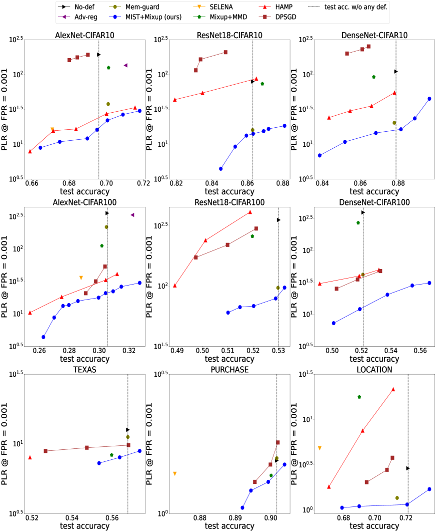
Figure 1: Comparing all defenses using the highest MI attack PLR @ 0.001 FPR among all evaluated attacks. Defenses placed at the lower right corner are better (high test accuracy and low PLR). Notice that for PURCHASE, TEXAS and LOCATION datasets the mixup data augmentation is not applied. We exclude some results when the testing accuracy drop is larger than $5\%$ for clearer comparison.

Dataset-Model	Defense	Train Acc.	Test Acc.	random-perturbation Attack PLR$\downarrow$ (FPR @ $0.1\%$)  [17]	LOSS Attack PLR$\downarrow$ (FPR @ $0.1\%$)  [45]	modified-entropy Attack PLR$\downarrow$ (FPR @ $0.1\%$)  [38]	class-NN Attack PLR$\downarrow$ (FPR @ $0.1\%$)  [37]	LIRA Attack PLR$\downarrow$ (FPR @ $0.1\%$) [3]	CANARY Attack PLR$\downarrow$ (FPR @ $0.1\%$) [42]
CIFAR-10, AlexNet	No-def	0.9989	0.6960	0.00	0.00	0.00	33.19	49.81	193.10
CIFAR-10, AlexNet	Adv-reg	0.9781	0.7103	0.00	0.00	0.00	21.88	12.18	135.38
CIFAR-10, AlexNet	Memguard	0.9930	0.7010	0.00	0.15	0.15	4.67	37.67	OOT
CIFAR-10, AlexNet	DMP	0.4141	0.4043	0.00	0.38	0.50	1.07	1.23	0.99
CIFAR-10, AlexNet	Mixup+MMD	0.8805	0.7012	0.00	0.10	0.12	1.25	26.29	125.18
CIFAR-10, AlexNet	SELENA	0.7250	0.6710	0.00	0.22	0.30	1.49	6.38	16.25
CIFAR-10, AlexNet	HAMP	0.8615	0.7106	0.00	0.12	0.12	1.06	10.15	33.58
CIFAR-10, AlexNet	DP-SGD	0.9881	0.6925	0.00	0.10	0.10	192.10	29.03	103.50
CIFAR-10, AlexNet	MIST +mixup	0.7589	0.7006	0.00	0.10	0.10	3.36	11.82	21.93
CIFAR-10, ResNet18	No-def	0.9991	0.8631	0.00	0.00	0.00	15.30	23.99	79.30
CIFAR-10, ResNet18	Adv-reg	MNC	MNC	MNC	MNC	MNC	MNC	MNC	MNC
CIFAR-10, ResNet18	Memguard	0.9999	0.8630	0.00	0.00	0.00	4.61	15.96	OOT
CIFAR-10, ResNet18	DMP	0.6973	0.6745	0.00	0.49	0.59	1.19	1.37	4.48
CIFAR-10, ResNet18	Mixup+MMD	0.9630	0.8685	0.00	0.05	0.10	4.58	12.07	73.60
CIFAR-10, ResNet18	SELENA	OOT	OOT	OOT	OOT	OOT	OOT	OOT	OOT
CIFAR-10, ResNet18	HAMP	0.9957	0.8651	0.00	0.00	0.00	2.65	22.61	87.38
CIFAR-10, ResNet18	DP-SGD	0.9797	0.8719	0.00	0.00	0.00	254.81	6.02	34.78
CIFAR-10, ResNet18	MIST +mixup	0.8802	0.8633	0.00	0.10	0.10	1.39	4.81	14.13
CIFAR-10, DenseNet	No-def	0.9995	0.8788	0.00	0.00	0.00	291.60	30.11	110.49
CIFAR-10, DenseNet	Adv-reg	0.2891	0.2841	0.00	0.00	0.00	0.54	0.89	1.01
CIFAR-10, DenseNet	Memguard	0.9999	0.8779	0.00	0.00	0.00	9.52	20.34	OOT
CIFAR-10, DenseNet	DMP	0.4845	0.4785	0.00	0.38	1.17	2.72	3.49	3.89
CIFAR-10, DenseNet	Mixup+MMD	0.9577	0.8671	0.00	0.10	0.10	48.31	27.31	92.34
CIFAR-10, DenseNet	SELENA	OOT	OOT	OOT	OOT	OOT	OOT	OOT	OOT
CIFAR-10, DenseNet	HAMP	0.9639	0.8780	0.00	0.10	0.19	6.34	19.15	55.12
CIFAR-10, DenseNet	DP-SGD	0.9898	0.8644	0.00	0.00	0.00	253.19	7.99	27.69
CIFAR-10, DenseNet	MIST +mixup	0.9097	0.8814	0.00	0.10	0.15	1.62	5.21	16.38

Table 1: Defense evaluation on CIFAR-10. OOT stands for out-of-time. The SELENA defense cannot be evaluated on ResNet18 and DenseNet because this defense requires more than half an year to run the experiments. The Memguard defense cannot be evaluated against CANARY attack also because of time constraint. MNC stands for Model Not Converging (training failure). Adv-reg failed on CIFAR-10, ResNet18. Lower PLR while preserving test accuracy is better.

Dataset-Model	Defense	Train Acc.	Test Acc.	random-perturbation Attack PLR$\downarrow$ (FPR@ $0.1\%$)  [17]	LOSS Attack PLR$\downarrow$ (FPR@ $0.1\%$)  [45]	modified-entropy Attack PLR$\downarrow$ (FPR@ $0.1\%$)  [38]	class-NN Attack PLR$\downarrow$ (FPR@ $0.1\%$)  [37]	LIRA Attack PLR$\downarrow$ (FPR@ $0.1\%$)[3]	CANARY Attack PLR$\downarrow$ (FPR@ $0.1\%$)[42]
CIFAR-100, AlexNet	No-def	0.9989	0.3054	0.00	0.00	0.00	93.96	171.95	357.37
CIFAR-100, AlexNet	Adv-reg	0.9822	0.3222	0.00	0.00	0.00	38.36	247.44	335.18
CIFAR-100, AlexNet	Memguard	0.9999	0.3048	0.00	0.00	0.00	55.67	218.70	OOT
CIFAR-100, AlexNet	DMP	MNC	MNC	MNC	MNC	MNC	MNC	MNC	MNC
CIFAR-100, AlexNet	Mixup+MMD	0.5473	0.3018	0.00	0.10	0.13	6.10	103.38	112.11
CIFAR-100, AlexNet	SELENA	0.3373	0.2879	0.00	0.15	0.20	2.68	20.99	35.09
CIFAR-100, AlexNet	HAMP	0.5959	0.3147	0.00	0.13	0.19	3.89	31.50	86.93
CIFAR-100, AlexNet	DP-SGD	0.5029	0.2977	0.00	0.33	0.40	10.38	18.87	31.75
CIFAR-100, AlexNet	MIST +mixup	0.3535	0.3049	0.00	0.14	0.19	6.92	17.43	9.45
CIFAR-100, ResNet18	No-def	0.9999	0.5301	0.00	0.00	0.00	55.40	104.52	354.18
CIFAR-100, ResNet18	Adv-reg	0.5491	0.4455	0.00	0.20	0.20	0.82	3.61	10.29
CIFAR-100, ResNet18	Memguard	0.9999	0.5298	0.00	0.00	0.00	15.53	96.82	OOT
CIFAR-100, ResNet18	DMP	0.1585	0.1490	0.00	0.28	0.39	29.43	1.06	2.64
CIFAR-100, ResNet18	Mixup+MMD	0.8883	0.5197	0.00	0.00	0.00	3.83	186.31	259.35
CIFAR-100, ResNet18	SELENA	OOT	OOT	OOT	OOT	OOT	OOT	OOT	OOT
CIFAR-100, ResNet18	HAMP	0.9851	0.5188	0.00	0.20	0.20	20.11	236.08	412.31
CIFAR-100, ResNet18	DP-SGD	0.9804	0.5212	0.00	0.00	0.00	11.35	66.32	300.40
CIFAR-100, ResNet18	MIST +mixup	0.5389	0.5202	0.00	0.10	0.13	5.49	27.60	68.34
CIFAR-100, DenseNet	No-def	1.0000	0.5211	0.00	0.00	0.00	20.21	120.10	395.27
CIFAR-100, DenseNet	Adv-reg	0.2891	0.2858	0.00	0.00	0.00	1.03	0.48	0.89
CIFAR-100, DenseNet	Memguard	1.0000	0.5209	0.00	0.00	0.00	1.48	42.07	OOT
CIFAR-100, DenseNet	DMP	0.0682	0.0665	0.00	0.00	0.00	1.10	1.05	1.13
CIFAR-100, DenseNet	Mixup+MMD	0.8286	0.5177	0.00	0.18	0.23	200.09	99.16	272.22
CIFAR-100, DenseNet	SELENA	OOT	OOT	OOT	OOT	OOT	OOT	OOT	OOT
CIFAR-100, DenseNet	HAMP	0.8397	0.5184	0.00	0.10	0.10	16.48	34.73	40.07
CIFAR-100, DenseNet	DP-SGD	0.8350	0.5103	0.00	0.15	0.15	0.59	21.49	35.55
CIFAR-100, DenseNet	MIST +mixup	0.5577	0.5188	0.00	0.20	0.20	1.20	17.47	12.10

Table 2: Defense evaluation CIFAR-100. OOT stands for out-of-time. The SELENA defense cannot be evaluated on ResNet18 and DenseNet because this defense requires more than half an year to run the experiments. The Memguard defense cannot be evaluated against CANARY attack also because of time constraint. MNC stands for Model Not Converging (training failure). DMP failed on CIFAR-100, AlexNet. Lower PLR while preserving test accuracy is better.

Dataset-Model	Defense	Train Acc.	Test Acc.	random-perturbation Attack PLR$\downarrow$ (FPR@ $0.1\%$)  [17]	LOSS Attack PLR$\downarrow$ (FPR@ $0.1\%$)  [45]	modified-entropy Attack PLR$\downarrow$ (FPR@ $0.1\%$)  [38]	class-NN Attack PLR$\downarrow$ (FPR@ $0.1\%$)  [37]	LIRA Attack PLR$\downarrow$ (FPR@ $0.1\%$) [3]	CANARY Attack PLR$\downarrow$ (FPR@ $0.1\%$) [42]
Texas	No-def	0.6955	0.5679	0.00	0.22	1.05	12.64	1.31	N/A
Texas	Adv-reg	0.3205	0.3081	0.00	0.00	0.00	4.76	1.23	N/A
Texas	Memguard	0.6955	0.5689	0.00	0.17	0.28	11.22	1.30	N/A
Texas	DMP	MNC	MNC	MNC	MNC	MNC	MNC	MNC	MNC
Texas	MMD	0.6397	0.5598	0.00	0.23	0.23	8.33	1.63	N/A
Texas	SELENA	0.5914	0.5366	0.00	0.10	0.15	8.14	1.48	N/A
Texas	HAMP	0.5346	0.5190	0.00	0.25	0.35	8.01	0.79	N/A
Texas	DP-SGD	0.6984	0.5682	0.00	0.03	0.03	9.80	1.18	N/A
Texas	MIST	0.6396	0.5638	0.00	0.23	0.39	8.01	1.29	N/A
Purchase	No-def	0.9998	0.9017	0.00	0.03	0.10	1.07	1.55	N/A
Purchase	Adv-reg	0.3692	0.3636	0.00	0.93	1.01	36.68	0.91	N/A
Purchase	Memguard	0.9999	0.9017	0.00	0.00	0.00	1.58	0.96	N/A
Purchase	DMP	MNC	MNC	MNC	MNC	MNC	MNC	MNC	MNC
Purchase	MMD	0.9897	0.9041	0.00	0.00	0.00	1.22	1.37	N/A
Purchase	SELENA	0.9234	0.8717	0.00	0.50	0.60	1.22	1.39	N/A
Purchase	HAMP	0.8926	0.8353	0.00	0.99	1.01	4.08	1.08	N/A
Purchase	DP-SGD	0.9893	0.8995	0.00	0.00	0.00	1.29	1.19	N/A
Purchase	MIST	0.9789	0.8944	0.00	0.05	0.05	1.08	0.67	N/A
Location	No-def	1.0000	0.7213	0.00	0.00	0.00	2.89	1.19	N/A
Location	Adv-reg	0.9447	0.6410	0.00	0.06	0.13	2.87	1.20	N/A
Location	Memguard	1.0000	0.7143	0.00	0.00	0.00	1.36	1.15	N/A
Location	DMP	MNC	MNC	MNC	MNC	MNC	MNC	MNC	MNC
Location	MMD	1.0000	0.6901	0.00	0.00	0.00	17.75	1.37	N/A
Location	SELENA	0.7307	0.6647	0.00	0.00	0.00	4.81	1.71	N/A
Location	HAMP	0.9885	0.7115	0.00	0.00	0.00	4.66	21.56	N/A
Location	DP-SGD	1.0000	0.7113	0.00	0.00	0.00	2.78	1.10	N/A
Location	MIST	0.9477	0.7159	0.00	0.00	0.00	0.71	1.15	N/A

Table 3: Our proposed defense evaluation on binary feature datasets. OOT stands for out-of-time. N/A stands for not applicable. The CANARY attack is not applicable to PURCHASE, TEXAS and LOCATION dataset because these three datasets only contain binary features. MNC stands for Model Not Converging (training failure). The DMP defense failed on all three binary datasets. Lower PLR while preserving test accuracy is better.

4.1.2 Evaluated Attacks and defenses

Attacks. We consider the six attacks described in Section 2.1: LOSS [45], Modified Entropy [38], Class-NN [37], random perturbation attack from [17], the online version of the LIRA attack from [3] and the CANARY attack from  [42]. Readers may want to review Section 2.1 on how these attacks work. The latter two are the state-of-the-art blackbox membership inference attack. We set the number of shadow models to be $100$, which is common in the literature. We assume that the attackers are adaptive attackers, which means that the attackers already know MIST defense mechanism (including hyperparameters) and can train similar models in exactly the same setting.

Defenses. We compare with the following existing defenses: adversarial regularization (adv-reg) [28], Mem-guard [18], DMP [36], Mixup+MMD [20], SELENA [39], HAMP [5] and DP-SGD [1]. Readers may want to review Section 2.2 on how these defense methods work. As for our MIST defense, we use the following setting: for $T_{1}$, we set it to be the number so that each data instance in subset $D^{c}$ can be visited just once and we set $T_{2}=T_{1}$. The chosen $\lambda$ for each model and dataset is also listed in Table 7. We tune the $\lambda$ so that the testing accuracy drop is less than $1\%$.

4.1.3 Evaluation Metrics

Following existing literature [29, 3], we use a balanced evaluation set. For CIFAR-10 and CIFAR-100 datasets, we assume that the model trainer has 20,000 data instances to perform the model training. For PURCHASE dataset and TEXAS dataset, we assume the model trainer has 40,000 training data instances. For LOCATION dataset, we assume the model trainer has 4,000 training data. We mainly use PLR (positive likelihood ratio, which is the ratio between TPR and FPR where lower means a more effective defense) at a fixed low FPR as suggested in Carlini et al. [3] to evaluate different attacks. For completeness, we also include AUC (area under curve) scores in the Appendix.

4.2 The computational cost (time and memory) of defenses

Here we assume that all the hyperparameters are already chosen, and compare the time that that model optimization needs to produce a final usable model and predictions for the testing set. We run this comparison experiments on a server with one GTX-1080Ti GPU and we use CIFAR-100 on AlexNet as an example to compare. Table 4 shows our results, where we can see that MIST achieves the second fastest running time among all defenses (only slower than HAMP defense). Note that the SELENA defense requires significantly more time to train a model comparing to the other two defenses, since it needs to train many extra models (25 with the code’s default parameters). Moreover, the Memguard defense also requires significant time, because the noise for each prediction needs to be optimized separately. As for memory cost of our MIST defense, it depends on the number of submodels (usually $2$ to $4$). In addition, we can see that SELENA requires more memories, again due to its significant number of models to be trained. In conclusion, our MIST only requires moderate extra time and memory for model training where the best privacy-utility tradeoff is provided. Besides, our method is better designed for multi-gpu scenarios, where each GPU contains one model associated with one data subset. Since we have found that 2 to 4 subsets are enough, the overall number of GPUs required is 2x to 4x of a standard method. Moreover, at each epoch our proposed method performs two backprop steps instead of one, and evaluates all the models on the whole dataset. This results in time overhead of a factor of 2x to 4x overall.

Defense name	Running time (s)	memory cost factor
SGD baseline	1195	1
Adv-reg	7008	1
DMP	2543	2
Memguard	36373	1
SELENA	20320	26
Mixup+MMD	3154	1
HAMP	1280	1
MIST +mixup	2139	4

Table 4: Computational cost comparison for different defenses. For memory cost, we only count the number of models to be trained.

4.3 Defense Effectiveness Evaluation

In our experiments, we try to make sure the testing accuracy drop is less than $1\%$ for all defenses. For some cases this is not possible, in which case we present the highest test accuracy possible.

In Figure 1 we summarize the evaluation of all defenses, by plotting all data points when the testing accuracy drop is no more than than $5\%$ for clearer comparison. All the detailed PLR numbers are presented in Sections 4.1.1, 4.1.1 and 4.1.1.

In Figure 1, the $x$-axis gives testing accuracy and the $y$-axis gives PLR_0.001 (PLR when FPR$=0.001$) in log-scale. We prefer methods to be in the lower-right region, as they can provide higher testing accuracy under the same PLR_0.001. Note that our proposed defense method MIST+Mixup performs the best in all experiments.

When PLR${}_{0.001}=100$, it means that when we ensure that no more than 0.1% of non-members are falsely identified as members, if we identify 101 instances as members, we can expect that 100 are indeed members, and 1 of them is a false positive. When PLR${}_{0.001}=2$, it means that when we ensure that no more than 0.1% of non-members are falsely identified as members, if we identify 3 as members, we can expect 2 of them are indeed members.

Effect of MIST+Mixup. We first look at how well our proposed defense (MIST+Mixup) prevents MI attacks. For CIFAR-10, our defense can reduce the highest PLR among all attacks from $127.63$ to $17.48$ (averaged over all models); for CIFAR-100 dataset, our defense can reduce the highest PLR from $368.94$ to $29.97$ (averaged over all models). For PURCHASE dataset, TEXAS dataset and LOCATION dataset, the highest PLR is reduced from $6.51$ to $4.10$, $1.55$ to $1.08$, $2.89$ to $1.15$ respectively. The PLR reduction is not huge since the model trained without any defense is already “safe” with the highest PLR already small. As for the average case attack effectiveness, our defense can also provide noticeable AUC drop comparing to the case without any defense, which is detailed in Appendices C, C and C in the Appendix. In summary, our new defense can provide significant attack effectiveness (including PLR and AUC) reduction for highly vulnerable cases (CIFAR-10 and CIFAR-100) and provide further attack effectiveness reduction on less vulnerable cases (PURCHASE, TEXAS and LOCATION), while incurring less than $1\%$ testing accuracy drop.

Comparison with adv-reg. In Sections 4.1.1, 4.1.1 and 4.1.1, we note that the adversarial regularization defense incurs significant testing accuracy drop for all cases except CIFAR-10, AlexNet and CIFAR-100, AlexNet. However, for these two cases, MIST+mixup (blue curve) provides much lower PLR than adversarial regularization (purple dot) when similar testing accuracy is achieved, as shown in Figure 1. Comparison with Memguard. The Memguard defense is a post-processing defense, which means the model utility (testing accuracy in our case) is maintained. From Figure 1, we can conclude that MIST+mixup (blue curve) provides lower PLR than Memguard (olive dot) when similar testing accuracy is achieved. We note that due to computational resources and time constraint, we are not able to evaluate Memguard against the CANARY attack, since the CANARY attack involves instance optimization through multiple iterations and for each iteration the Memguard defense needs to calculate a new noise regarding each newly perturbed instance. If we only compare the PLR of the LIRA attack, we can see that MIST+mixup outperforms Memguard for all cases. Moreover, the PLR of the CANARY attack against MIST+mixup is still lower than the PLR of the LIRA attack against Memguard for all CIFAR experiments.

Comparison with DMP. In this comparison, we consider the case where no auxiliary unlabeled data is available because in practice collecting extra data is intractable for most privacy-concerning cases, for example medical images. More specifically, we train a GAN using the private training set and draw samples using the trained GAN to train the student model. In Sections 4.1.1, 4.1.1 and 4.1.1, we see that the DMP defense also incurs significant testing accuracy drop comparing to the no-def case. Comparison with Mixup+MMD. From Figure 1, we can conclude that MIST+mixup (blue curve) provides lower PLR than Mixup+MMD (green dot) when similar testing accuracy is achieved. For Mixup+MMD defense, more interestingly, we realize that our proposed cross-difference loss is similar to the MMD (mean maximum discrepancy) loss proposed in Li et al. [20]. The only difference is the granularity, i.e., our proposed cross-difference loss is calculated on instance level, but the MMD loss is calculated on class level, where the loss is defined as the difference between averages of two classes. For that reason, our proposed cross-difference loss should outperform the MMD loss.

Comparison with SELENA. We first note that the SELENA defense and its evaluation against shadow-model based attacks require extraordinarily large amount of computational resources. This is because the SELENA defense needs to train $25$ (the default value) models and then train one distilled model from these $25$ models. Moreover, if we want to evaluate the LIRA attack against the SELENA defense and the number of shadow models is $100$, then we need to perform the SELENA training procedure for $100$ times to generate $100$ distilled models and in total we need to train $2600$ models for all our models and datasets, which is unattainable in our experimental scenario where each model is not small. Thus, for our experiments we restrict SELENA defense evaluation to the following scenarios: CIFAR-10 with AlexNet, CIFAR-100 with AlexNet, PURCHASE, TEXAS and LOCATION. From Figure 1, we can conclude that MIST+mixup defense (blue curve) provides lower PLR and higher testing accuracy than SELENA defense (yellow dot). Particularly for the TEXAS dataset, the SELENA defense results in more than $25\%$ testing accuracy drop, thus we exclude this data point from Figure 1 for clearer comparison. One reason that our defense can outperform SELENA is that, during the training process, there is communication (regularizing each other and averaging parameters) between each submodels, however SELENA does not have communication between submodels. We note that in Sections 4.1.1, 4.1.1 and 4.1.1 we report the results of our defense when the testing accuracy drop is less than $1\%$. Thus for the CIFAR-10 AlexNet case, the numbers of our defense are worse than the SELENA defense. However, this is not a fair comparison since the SELENA defense sacrifices more testing accuracy for better defense. The comparison is fair when both defenses produce the same testing accuracy.

Comparison with HAMP. For the HAMP defense, we only evaluate the effectiveness of their training-time defense, since the testing time defense can be integrated with any training time defenses and the testing time defense is approximately equivalent to providing the predicted label only. In Figure 1, if we compare MIST+mixup (blue curve) with HAMP (red curve), we can conclude that MIST+mixup gives better privacy-utility tradeoff than HAMP. For the HAMP defense, our defense considers the MI difficulty of different individual instances and regularize more on vulnerable instances, however the HAMP defense treats all instances in the same fashion by applying an entropy-based regularizer and smoothed label.

Comparison with DP-SGD. Note that for the DP-SGD defense we tune the hyperparameter so that the model trained with DP-SGD can achieve similar testing accuracy and in this case, the privacy budget is huge. In Figure 1, if we compare MIST+mixup (blue curve) with DP-SGD (brown curve), we can conclude that MIST gives better privacy-utility tradeoff than DP-SGD.

To summarize, our MIST defense can outperform all existing defenses for all evaluated cases. In addition, our defense also provides a “knob” (the parameters $\lambda$ and $T_{2}$ of Phase 2) to further fine-tune the model, so practitioners can obtain different tradeoffs between test accuracy and MI attack robustness. This tradeoff flexibility is absent from some of the baseline defenses, unfortunately.

4.4 Evaluating our proposed defense against label only MIAs

Now we evaluate the effectiveness of MIST against label-only MIAs from Choquette-Choo et al. [6]. Particularly, we evaluate the more effective adversarial perturbation label-only MIA. We use the AUC score to evaluate the effectiveness of the distance attack, since it is impossible to use PLR at low FPR to evaluate the distance attack due to its definition: wrongly classified instances have $0$ distance. The results are shown in Table 5. We can conclude that our proposed defense can significantly reduce the AUC score of the distance attack.

Dataset-Model	Defense	Attack AUC score
CIFAR-10, AlexNet	No Defense	0.641
CIFAR-10, AlexNet	MIST+mixup	0.536
CIFAR-100, AlexNet	No Defense	0.826
CIFAR-100, AlexNet	MIST+mixup	0.540

Table 5: Evaluation of our proposed defense against label only MIA. CIFAR dataset, AlexNet.

4.5 Choosing hyperparameters

Now we discuss how to determine the two most crucial hyperparameters of our proposed defense: the number of models and the weight of the cross-difference loss. In this paper, we use the following method to determine these two hyperparameters: we choose the number of models to achieve the highest validation accuracy possible and then choose the weight of the cross-difference loss to provide the strongest defense while making sure the testing accuracy drop is less than $1\%$ comparing to the base case without any defense. In Figure 5 in the Appendix (with more detailed results in Appendices C and C in the Appendix), we show that the customized subspace learning (without the cross-difference loss) can help the model generalize better, thus we would like to use the model with the highest validation accuracy. Moreover, the mixup data augmentation can also help to further improve the validation accuracy. Hence, subspace learning and mixup combined get higher test accuracy boost compared to standard SGD, which then gives us room to increase the regularization of the cross difference loss without lower test accuracy when compared against standard SGD.

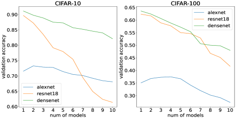
Figure 2: Validation accuracy v.s. number of models. Mixup data augmentation is applied.

In Figure 2, we show the validation accuracy curve v.s. the number of models for all models and datasets where mixup data augmentation is applicable. Recall that we need to choose the number of models that achieves the highest validation accuracy. However, we also need to have at least two models, so that our cross-difference loss is applicable. Thus, where mixup data augmentation is applicable, for all models and datasets except CIFAR-100 and AlexNet, the number of models should be $2$. For the CIFAR-100 and AlexNet, the number of models should be four. For the case where the mixup data augmentation is not applicable (TEXAS dataset and PURCHASE dataset), we choose to use 4 models for TEXAS dataset and 4 models for PURCHASE dataset based on Figure 5 in the Appendix. In practice, we recommend developers to generate this validation accuracy curve for their own datasets to determine the number of models. If the computational resources are limited, our ad-hoc advice is to use $2$ to $4$ models since this range was suitable for all our datasets.

As for the choice of the hyperparameter $\lambda$ of Phase 2 (the cross-difference loss minimization), we choose $\lambda$ as to provide the strongest defense while making sure the testing accuracy drop is less than $1\%$. In practice, the training does not need to follow this procedure, as $\lambda$ may be utilized as a knob to tune a privacy-utility tradeoff, which allow practitioners to determine this tradeoff based on their needs.

4.6 Ablation Study

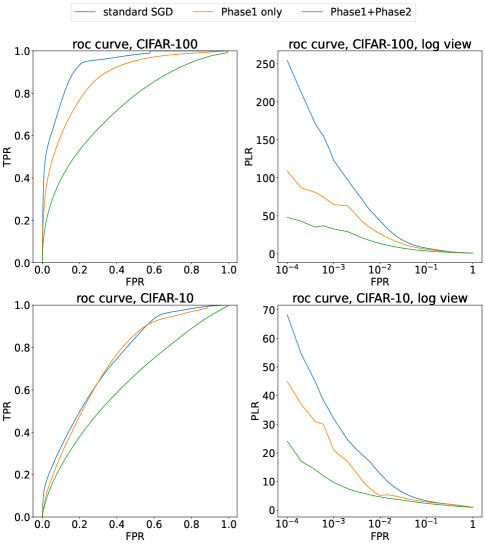
Figure 3: The clear positive impact of Phase 1 and Phase 2. Impact measured on ROC curve and PLR at low FPR region. LIRA attack is evaluated to produce the ROC curve and PLR curve. CIFAR-100 and CIFAR-10 using AlexNet.

The positive impact of subspace learning and cross-difference loss. In this ablation study, we use AlexNet on CIFAR-10 and CIFAR-100 dataset. For CIFAR-10 dataset, we use $3$ models and for CIFAR-100 dataset we use $7$ models. These two values are chosen because the highest testing accuracy (higher than the standard SGD case with one model) can be achieve with this choice when no cross-difference loss and mix-up data augmentation is applied (detailed results are shown in Appendices C and C in the Appendix). For the $\lambda$ of the cross difference loss, we choose the $\lambda$ so that the maximum defense can be provided while the testing accuracy drop is less than $1\%$ in this experiment. We compare the attack effectiveness against model trained without defense, trained with Phase 1 only and trained with both Phases 1 and 2. The results are shown in Figure 3. We can conclude that the only performing Phase 1 of our MIST algorithm (ignoring Phase 2) can still be used as a defense which can preserve utility and decrease attack effectiveness at the same time with appropriate number of models. We also repeat this experiment on other models and datasets and we observe similar phenomenon. Moreover, adding Phase 2 (cross-difference loss minimization) can provide further robustness against the LIRA attack.

Different cross-difference loss implementations. In this ablation study, we experiment on different implementations for the cross-difference loss. More specifically, we use three different implementations: KL-divergence, Equation 3 and $L_{2}$ version of Equation 3. We run experiments using AlexNet on CIFAR-100 dataset and we choose the optimal weights that we can find for each loss function so that the testing accuracy drop is less than $1\%$ comparing to the case without any defense. The results are shown in Table 6, where we can conclude that the $L_{1}$ variant slightly outperforms the other two variants and the KL-divergence variant performs the worst. One possible reason for the KL-divergence variant being worse than $L_{1}$ is because the KL-divergence considers the distance between two prediction vectors, while the state-of-the-art attacks only focus on the probability of the correct label. Moreover, we also observe that this KL-divergence variant makes the model training unstable, meaning that sometimes the model fails to converge, thus we recommend the use of $L_{1}$.

Loss function	Testing accuracy	PLR at $0.1\%$ FPR
L1	0.3049	17.43
L2	0.2997	17.54
KL-divergence	0.3003	19.72

Table 6: Comparing different implementations of the MIST loss. CIFAR-100 dataset on AlexNet.

5 Conclusion

In this work we introduce Membership-Invariant Subspace Training (MIST), a method for training classifiers that acts as a defense designed to specifically defend against blackbox membership inference attacks on the most vulnerable instances in the training data (which also helps defending against overall blackbox MI attacks). MIST uses a novel two-phase subspace learning procedure that trains models regularized to be membership invariant (counterfactually invariant to the membership of each instance in the training data $D$). Through our proposed two-phase subspace learning method, and a new proposed loss (cross-difference loss), we can efficiently regularize neural network training towards membership-invariant classifiers. Our experiments empirically show that our trained classifiers are significantly less vulnerable against blackbox membership inference attacks than baselines, especially on those most vulnerable training examples.

Appendix A Further Related Work

Other MI attacks that are similar to LIRA but weaker. Several MI attacks are similar to LIRA and are shown in  [3] to be less effective in LIRA; we thus do not consider them in the experiments. We list these attacks below.

Long et al. [24] proposed to train instance-specific MI classifiers. For each instance $x$, there will be two sets of models: trained with $x$ and trained without $x$. Then, the average prediction of $x$ from the member set and the average prediction of $x$ from the non-member set is calculated. $x$ is predicted to be a member if the target model’s prediction of $x$ is more similar to the average prediction of the member set (in the sense of KL divergence).

Ye et al. [44] followed the same shadow model procedure as  [41] to produce a collection of loss for one instance when this instance is not used in the training. Next, a one-sided hypothesis testing is proposed to predict membership. The advantage of this hypothesis testing is that the attacker could select a false positive rate. However, the possible false positive rate range is limited by the number of shadow models. Watson et al. [41] propose to use the shadow models to set a per-instance loss threshold by the average of loss of the instance on shadow models that are not trained using this example.

Other membership inference defenses. In  [37], it was proposed to reduce the information given by the prediction vectors, such as providing only the top-k probabilities and using high temperature in softmax. This has limited effectiveness as the top-k probabilities give enough information needed by the best attacks, and high temperatures change only the absolute values of confidences, but not the fact that confidences for members tend to be higher than that for non-members. Moreover, this defense is not effective against LIRA, thus we do not consider this defense in our experiments.

Membership inference attacks in other settings. Melis et al. [26] identified membership leakage when using FL for training a word embedding function, which is a deterministic function that maps each word to a high-dimensional vector. Given a training batch (composed of sentences), the gradients are all $0$’s for the words that do not appear in this batch, and thus the set of words used in the training sentences can be inferred. The attack assumes that the participants update the central server after each mini-batch, as opposed to updating after each training epoch.

Nasr et al. [29] use gradient updates as feature vectors and train an auto-encoder to generate a single-number embedding to predict membership. This attack was also applied in the white-box setting, for which it performs worse than attacks that directly use gradient norm to predict membership, which show only small improvement over blackbox attacks. Another interesting idea in [29] is that a malicious server can actively improve MI attacks, by applying a gradient ascent with respect to the target instance. If the instance is a member, then the gradients tend to be larger in order to compensate for the malicious gradient ascent.

Li et al. [21] proposed a new membership inference attack against the federated learning setting. They observed that the cosine similarity between gradients of each data instance and the parameter updates sent by each client has very different distribution for members and non-members. Thus, the cosine similarity is used as the metric to predict members. They also proposed to use the gradient difference between the gradients of each data instance and the parameter updates to predict membership. Their results show that the new proposed attacks can achieve higher TPR at low FPR than the attack proposed in  [29].

Song et al. [38] evaluated how adversarial training would affect the privacy leakage. Experiments showed that adversarial training would boost the performance of instance loss membership inference attack and the testing accuracy of the target model will be decreased.

Liu et al. [23] evaluated the privacy leakage of pre-trained models which are trained using unsupervised contrastive learning strategy. The authors proposed a specific membership inference attack against pre-trained models. Given one instance, this new attack generates many perturbed versions of this instance and gather all the embeddings of these perturbed versions using the pre-trained model. The intuition is if one instance is used in the training of this pre-trained model, then the embeddings of its perturbed versions are generally closer to each other. He et al. [13] utilized the same contrastive learning idea and proposed to fine-tune the pre-trained model to get the final target model. Experiments showed that using pre-trained model as feature extractor would reduce privacy leakage, comparing to training models from scratch.

Hidano et al. [14] evaluated MI attack under the setting where the attacker can know the parameters of some shallow layers. In the experiment, the author assumed that the attacker can get all but the last layer and the parameters of these layers are used to initialize shadow models to facilitate the class-vector attack. With these known parameters, the class-vector attack can outperform its black-box version.

Other privacy-threatening attacks. Salem et al. [34] studied the possible information leakage of an update set when the machine learning model is updated using the update set. To detect the information leakage, the authors proposed two different attacks: label inference attack and instance reconstruction attack. These two attacks can be applied to both single instance update set case and multi-instances update set case, with only black-box access to the machine learning model.

Zhu et al. [47] presented a gradient-based instance reconstruction attack. If the gradients of one specific instance are revealed to one adversary who can access the trained model, then the adversary is able to reconstruct the specific instance with high fidelity. One random instance is gradually optimized by matching its gradients with the provided gradients of the specific instance.

Appendix B Additional Ablation Study

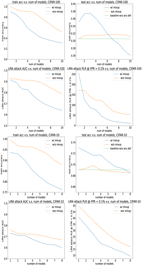
Figure 4: The impact of mixup data augmentation on training accuracy, testing accuracy and attack effectiveness when the number of models is varied. AlexNet, CIFAR-10 and CIFAR-100 datasets.

The positive impact of mixup data augmentation. The experiment is performed using CIFAR-10 and CIFAR-100 dataset on AlexNet. We perform experiments while varying the number of models $K$ from 1 to 8 for CIFAR-10 (10 for CIFAR-100). $D$, which contains 20,000 training instances, is divided into $K$ equal-size, disjoint partitions, and each model will be trained using one partition for one epoch, before we average the model. For each number of models choice, we experiment with two cases: with mixup and without mixup. The results are shown in Figure 4. The detailed numbers are included in Table C, C, C and C in the appendix. From Figure 4, for CIFAR-100 dataset, the first thing we can observe is that the training accuracy is decreased and the testing accuracy is increased when mixup is applied for the same number of models. Furthermore, by adding the mixup data augmentation, the LIRA attack AUC and LIRA attack PLR at low FPR are both reduced when the same number of models are created. This validates the effectiveness of the mixup data augmentation. However, we also noticed that the testing accuracy is always decreasing while creating more than one models and when the number of models is seven, the testing accuracy is very similar to the testing accuracy when there is no defense. Thus, there is a privacy-utility tradeoff that should be considered by the model trainer and the model trainer should choose the number of models based on their own needs. In addition, in order to regularize the trained model with the cross-difference loss, there should be at least two models. For CIFAR-10 dataset, we also notice that the training accuracy is decreased and the testing accuracy is increased when mixup is applied for the same number of models, which again verifies the effectiveness of the mixup data augmentation. The only difference is that, the testing accuracy increases and then decreases while having more models. Therefore, we suggest the model trainers to generate similar figures like Figure 4 and choose the number of models based on their needs.

Appendix C Additional Experimental Details and Results

Hyperparameters. In Table 7, we present all the hyperparameters used in our evaluation.

Detailed numbers for all defenses evaluation. In Table C, C and C we present the detailed AUC numbers for the evaluation of all defenses.

dataset	model	lr	epochs	schedule	batch size	number of models	lambda
CIFAR-10	AlexNet	0.05	120	[100]	100	2	3.5
CIFAR-10	ResNet-18	0.10	300	[200,250]	100	2	3.5
CIFAR-10	DenseNet_BC(100,12)	0.10	500	[300,350]	100	2	6.0
CIFAR-100	AlexNet	0.05	120	[100]	100	4	12.0
CIFAR-100	ResNet-18	0.10	300	[200,250]	100	2	13.0
CIFAR-100	DenseNet_BC(100,12)	0.10	500	[300,350]	100	2	13.0
PURCHASE-100	PURCHASE-100	0.10	100	None	100	4	40.0
TEXAS-100	TEXAS-100	0.10	100	None	100	4	25.0
LOCATION	LOCATION	0.10	100	None	100	4	14.0

Table 7: Training recipe for different models. Learning rate is adjusted to 0.1x when current epoch is in schedule.

Dataset-Model	Defense	Train Acc.	Test Acc.	random-perturbation Attack AUC  [17]	LOSS Attack AUC  [45]	modified-entropy Attack AUC  [38]	class-NN Attack AUC  [37]	LIRA Attack AUC  [3]	CANARY Attack AUC  [42]
CIFAR-10, AlexNet	No-def	0.9989	0.6960	0.5000	0.7075	0.7101	0.7221	0.7598	0.8803
CIFAR-10, AlexNet	Adv-reg	0.9980	0.7103	0.5000	0.6558	0.6694	0.6728	0.7454	0.8256
CIFAR-10, AlexNet	Memguard	0.9930	0.7010	0.5000	0.6225	0.6275	0.6396	0.7259	OOT
CIFAR-10, AlexNet	DMP	0.4141	0.4043	0.5010	0.5077	0.5088	0.5044	0.5067	0.5129
CIFAR-10, AlexNet	Mix-up+MMD	0.8805	0.7012	0.5000	0.6322	0.6382	0.6470	0.7014	0.8050
CIFAR-10, AlexNet	SELENA	0.7250	0.6710	0.5000	0.5488	0.5483	0.5038	0.6338	0.6415
CIFAR-10, AlexNet	HAMP	0.8615	0.7106	0.5000	0.5895	0.5900	0.5854	0.6475	0.7559
CIFAR-10, AlexNet	DP-SGD	0.9881	0.6925	0.5001	0.7032	0.7138	0.7160	0.7634	0.8687
CIFAR-10, AlexNet	Mix-up+MIST	0.7589	0.7006	0.5000	0.5838	0.5830	0.5878	0.6295	0.7237
CIFAR-10, ResNet18	No-def	0.9991	0.8631	0.5000	0.6144	0.6133	0.6159	0.6684	0.7775
CIFAR-10, ResNet18	Adv-reg	MNC	MNC	MNC	MNC	MNC	MNC	MNC	MNC
CIFAR-10, ResNet18	Memguard	0.9999	0.8630	0.5000	0.5830	0.5820	0.5691	0.6157	OOT
CIFAR-10, ResNet18	DMP	0.6973	0.6745	0.5000	0.5151	0.5167	0.5161	0.5084	0.5199
CIFAR-10, ResNet18	Mix-up+MMD	0.9630	0.8685	0.5000	0.5770	0.5780	0.6221	0.6122	0.7640
CIFAR-10, ResNet18	SELENA	OOT	OOT	OOT	OOT	OOT	OOT	OOT	OOT
CIFAR-10, ResNet18	HAMP	0.9957	0.8651	0.5000	0.6290	0.6293	0.6350	0.6830	0.7890
CIFAR-10, ResNet18	DP-SGD	0.9797	0.8719	0.5000	0.5749	0.5788	0.6203	0.6190	0.6879
CIFAR-10, ResNet18	Mix-up+MIST	0.8802	0.8633	0.5000	0.5623	0.5666	0.5690	0.5795	0.6516
CIFAR-10, DenseNet	No-def	0.9995	0.8788	0.5000	0.6208	0.6201	0.6178	0.6932	0.7575
CIFAR-10, DenseNet	Adv-reg	0.2891	0.2841	0.5000	0.5037	0.5040	0.5079	0.5028	0.5088
CIFAR-10, DenseNet	Memguard	0.9999	0.8788	0.5000	0.5736	0.5739	0.5760	0.6375	OOT
CIFAR-10, DenseNet	DMP	0.4845	0.4785	0.5000	0.5031	0.5047	0.5020	0.5040	0.5091
CIFAR-10, DenseNet	Mix-up+MMD	0.9577	0.8671	0.5000	0.5851	0.5890	0.5919	0.6744	0.7434
CIFAR-10, DenseNet	SELENA	OOT	OOT	OOT	OOT	OOT	OOT	OOT	OOT
CIFAR-10, DenseNet	HAMP	0.9639	0.8780	0.5000	0.5680	0.5701	0.5893	0.6397	0.6918
CIFAR-10, DenseNet	DP-SGD	0.9898	0.8644	0.5000	0.5848	0.5830	0.5818	0.6319	0.6867
CIFAR-10, DenseNet	Mix-up+MIST	0.9097	0.8814	0.5000	0.5758	0.5799	0.5783	0.5991	0.6676

Table 8: Our proposed defense evaluation on CIFAR-10. OOT stands for out-of-time. The SELENA defense cannot be evaluated on ResNet18 and DenseNet because this defense requires more than half an year to run the experiments. The Adv-reg defense encounters training failure on CIFAR-10, ResNet. MNC stands for Model Not Converging (training failure).

Dataset-Model	Defense	Train Acc.	Test Acc.	random-perturbation Attack AUC  [17]	LOSS Attack AUC  [45]	modified-entropy Attack AUC  [38]	class-NN Attack AUC  [37]	LIRA Attack AUC  [3]	CANARY Attack AUC  [42]
CIFAR-100, AlexNet	No-def	0.9989	0.3054	0.5000	0.8899	0.8920	0.9002	0.9242	0.9836
CIFAR-100, AlexNet	Adv-reg	0.9822	0.3222	0.5000	0.8888	0.9010	0.9023	0.9482	0.9834
CIFAR-100, AlexNet	Memguard	0.9999	0.3048	0.5000	0.8849	0.8890	0.9155	0.9593	OOT
CIFAR-100, AlexNet	DMP	MNC	MNC	MNC	MNC	MNC	MNC	MNC	MNC
CIFAR-100, AlexNet	Mix-up+MMD	0.5473	0.3018	0.5000	0.7249	0.7299	0.7239	0.8089	0.9396
CIFAR-100, AlexNet	SELENA	0.3373	0.2879	0.5000	0.5917	0.5901	0.6014	0.6644	0.7142
CIFAR-100, AlexNet	HAMP	0.5959	0.3147	0.5000	0.6990	0.7120	0.7046	0.8120	0.8604
CIFAR-100, AlexNet	DP-SGD	0.5029	0.2977	0.5002	0.6637	0.6710	0.6739	0.7014	0.8199
CIFAR-100, AlexNet	Mix-up+MIST	0.3535	0.3049	0.5000	0.5619	0.5693	0.5782	0.6412	0.7714
CIFAR-100, ResNet18	No-def	0.9999	0.5301	0.5000	0.8885	0.8899	0.9012	0.9270	0.9695
CIFAR-100, ResNet18	Adv-reg	0.5491	0.4455	0.5000	0.5830	0.5830	0.5719	0.5721	0.6320
CIFAR-100, ResNet18	Memguard	0.9999	0.5298	0.5000	0.7529	0.7623	0.7727	0.8669	OOT
CIFAR-100, ResNet18	DMP	0.1585	0.1490	0.5000	0.5113	0.5122	0.6521	0.5043	0.5139
CIFAR-100, ResNet18	Mix-up+MMD	0.8883	0.5197	0.5000	0.7845	0.7855	0.7910	0.9028	0.9288
CIFAR-100, ResNet18	SELENA	OOT	OOT	OOT	OOT	OOT	OOT	OOT	OOT
CIFAR-100, ResNet18	HAMP	0.9851	0.5188	0.5000	0.8308	0.8281	0.8502	0.9391	0.9710
CIFAR-100, ResNet18	DP-SGD	0.9804	0.5212	0.5000	0.7793	0.7801	0.7905	0.8552	0.9384
CIFAR-100, ResNet18	Mix-up+MIST	0.5389	0.5202	0.5000	0.5877	0.5937	0.6394	0.6826	0.8288
CIFAR-100, DenseNet	No-def	1.0000	0.5211	0.5000	0.8617	0.8610	0.8649	0.9270	0.9615
CIFAR-100, DenseNet	Adv-reg	0.2891	0.2858	0.5000	0.5038	0.5047	0.5019	0.5060	0.5070
CIFAR-100, DenseNet	Memguard	1.0000	0.5209	0.5000	0.7588	0.7601	0.7748	0.8469	OOT
CIFAR-100, DenseNet	DMP	0.0682	0.0665	0.5000	0.5031	0.5048	0.5081	0.5093	0.5101
CIFAR-100, DenseNet	Mix-up+MMD	0.8286	0.5177	0.5000	0.8015	0.8103	0.8292	0.8385	0.9259
CIFAR-100, DenseNet	SELENA	OOT	OOT	OOT	OOT	OOT	OOT	OOT	OOT
CIFAR-100, DenseNet	HAMP	0.8397	0.5184	0.5000	0.6864	0.6890	0.7564	0.7948	0.8257
CIFAR-100, DenseNet	DP-SGD	0.8350	0.5103	0.5000	0.6758	0.6794	0.6904	0.7418	0.7899
CIFAR-100, DenseNet	Mix-up+MIST	0.5577	0.5188	0.5000	0.5715	0.5839	0.5913	0.6868	0.7469

Table 9: Our proposed defense evaluation on CIFAR-100. OOT stands for out-of-time. The SELENA defense cannot be evaluated on ResNet18 and DenseNet because this defense requires more than half an year to run the experiments. The DMP defense encounters training failure on CIFAR-100, AlexNet. MNC stands for Model Not Converging (training failure).

Dataset-Model	Defense	Train Acc.	Test Acc.	random-perturbation Attack AUC  [17]	LOSS Attack AUC  [45]	modified-entropy Attack AUC  [38]	class-NN Attack AUC  [37]	LIRA Attack AUC  [3]	CANARY Attack AUC  [42]
Texas	No-def	0.6955	0.5679	0.5000	0.6117	0.6203	0.6840	0.6211	N/A
Texas	Adv-reg	0.3205	0.3081	0.5000	0.5136	0.5206	0.8450	0.5026	N/A
Texas	Memguard	0.6955	0.5689	0.5000	0.6186	0.6199	0.6735	0.5102	N/A
Texas	DMP	MNC	MNC	MNC	MNC	MNC	MNC	MNC	MNC
Texas	MMD	0.6397	0.5598	0.5000	0.5991	0.6001	0.6533	0.5545	N/A
Texas	SELENA	0.5914	0.5366	0.5000	0.5498	0.5499	0.6344	0.5479	N/A
Texas	HAMP	0.5346	0.5190	0.5010	0.5066	0.5109	0.7073	0.5019	N/A
Texas	DP-SGD	0.6892	0.5596	0.5000	0.6105	0.6115	0.6795	0.5789	N/A
Texas	MIST	0.6396	0.5638	0.5000	0.5800	0.5830	0.6379	0.5574	N/A
Purchase	No-def	0.9998	0.9017	0.5020	0.6171	0.6210	0.6351	0.6689	N/A
Purchase	Adv-reg	0.3692	0.3636	0.5000	0.5070	0.5080	0.5058	0.5004	N/A
Purchase	Memguard	0.9999	0.9017	0.5000	0.5287	0.5290	0.5298	0.5080	N/A
Purchase	DMP	MNC	MNC	MNC	MNC	MNC	MNC	MNC	MNC
Purchase	MMD	0.9897	0.9041	0.5000	0.6052	0.6039	0.6300	0.6564	N/A
Purchase	SELENA	0.9234	0.8717	0.5000	0.5460	0.5480	0.5320	0.6592	N/A
Purchase	HAMP	0.8926	0.8343	0.5000	0.5053	0.5038	0.5271	0.5004	N/A
Purchase	DP-SGD	0.9893	0.8995	0.5000	0.6233	0.6310	0.6422	0.6732	N/A
Purchase	MIST	0.9789	0.8944	0.5000	0.5975	0.5979	0.6150	0.5938	N/A
Location	No-def	1.0000	0.7213	0.5002	0.7753	0.7758	0.7688	0.9258	N/A
Location	Adv-reg	0.9447	0.6410	0.5010	0.6489	0.6481	0.6843	0.5708	N/A
Location	Memguard	1.0000	0.7143	0.5000	0.7716	0.7720	0.7475	0.7790	N/A
Location	DMP	MNC	MNC	MNC	MNC	MNC	MNC	MNC	MNC
Location	MMD	1.0000	0.6901	0.5000	0.6270	0.6239	0.8094	0.6139	N/A
Location	SELENA	0.7307	0.6647	0.5000	0.5116	0.5122	0.5079	0.5419	N/A
Location	HAMP	0.9885	0.7115	0.5109	0.6868	0.6910	0.6835	0.8959	N/A
Location	DP-SGD	1.0000	0.7113	0.5028	0.7827	0.7837	0.7797	0.8831	N/A
Location	MIST	0.9560	0.7159	0.5001	0.7120	0.7111	0.7583	0.7255	N/A

Table 10: Our proposed defense evaluation on binary feature datasets. OOT stands for out-of-time. N/A stands for not applicable. The CANARY attack is not applicable to PURCHASE, TEXAS and LOCATION dataset because these three datasets only contain binary features. MNC stands for Model Not Converging (training failure).

Figure 5: Testing accuracy v.s. number of models for all datasets and models considered in this paper. No mixup data augmentation. The main observation is that testing accuracy can be improved by adding a few models. However, adding too many models would cost testing accuracy.

Dataset-Model	Number of models	Train Acc.	Test Acc.	LOSS Attack AUC	LIRA Attack AUC	LIRA Attack PLR (FPR @ $0.1\%$)
CIFAR-10, AlexNet	1	0.9948	0.6905	0.7213	0.7590	49.81
CIFAR-10, AlexNet	2	0.9678	0.6931	0.6870	0.7283	43.56
CIFAR-10, AlexNet	3	0.9631	0.6985	0.6831	0.7237	37.88
CIFAR-10, AlexNet	4	0.9620	0.6899	0.6729	0.7218	32.01
CIFAR-10, AlexNet	5	0.9473	0.6880	0.6590	0.7117	26.95
CIFAR-10, AlexNet	6	0.9291	0.6873	0.6444	0.6985	22.78
CIFAR-10, AlexNet	7	0.8991	0.6859	0.6211	0.6826	19.59
CIFAR-10, AlexNet	8	0.8790	0.6841	0.6113	0.6714	16.86

Table 11: Experimental results of varying number of models. CIFAR-10, AlexNet. No cross-difference loss, no mixup data augmentation.

Dataset-Model	Number of models	Train Acc.	Test Acc.	LOSS Attack AUC	LIRA Attack AUC	LIRA Attack PLR (FPR @ $0.1\%$)
CIFAR-100, AlexNet	1	0.9760	0.3054	0.8899	0.9242	171.95
CIFAR-100, AlexNet	2	0.9459	0.3142	0.8632	0.9230	170.46
CIFAR-100, AlexNet	3	0.9105	0.3156	0.8411	0.9114	140.80
CIFAR-100, AlexNet	4	0.9090	0.3123	0.8334	0.9087	123.34
CIFAR-100, AlexNet	5	0.8800	0.3149	0.8241	0.9086	121.36
CIFAR-100, AlexNet	6	0.8132	0.3164	0.7961	0.8954	95.31
CIFAR-100, AlexNet	7	0.7314	0.3173	0.7641	0.8729	70.19
CIFAR-100, AlexNet	8	0.6564	0.3108	0.7268	0.8423	61.30
CIFAR-100, AlexNet	9	0.5788	0.3161	0.6843	0.8147	55.59
CIFAR-100, AlexNet	10	0.5223	0.3125	0.6545	0.7874	53.28
CIFAR-100, AlexNet	11	0.4715	0.3008	0.6315	0.7629	43.00
CIFAR-100, AlexNet	12	0.4321	0.2920	0.6285	0.7394	36.33

Table 12: Experimental results of varying number of models. CIFAR-100 dataset, AlexNet. No cross-difference loss, no mixup data augmentation.

Dataset-Model	Number of models	Train Acc.	Test Acc.	LOSS Attack AUC	LIRA Attack AUC	LIRA Attack PLR (FPR @ $0.1\%$)
CIFAR-10, AlexNet	1	0.9360	0.7301	0.6535	0.7284	40.77
CIFAR-10, AlexNet	2	0.9305	0.7235	0.6548	0.7128	33.97
CIFAR-10, AlexNet	3	0.8980	0.7165	0.6238	0.7076	27.01
CIFAR-10, AlexNet	4	0.8517	0.7171	0.5935	0.6736	19.54
CIFAR-10, AlexNet	5	0.8211	0.7057	0.5705	0.6488	17.36
CIFAR-10, AlexNet	6	0.7940	0.6960	0.5632	0.6284	14.61
CIFAR-10, AlexNet	7	0.7773	0.6928	0.5583	0.6255	12.67
CIFAR-10, AlexNet	8	0.7616	0.6853	0.5506	0.5994	9.37

Table 13: Experimental results of varying number of models. Mix-up data augmentation is applied. CIFAR-10, AlexNet.

Dataset-Model	Number of models	Train Acc.	Test Acc.	LOSS Attack AUC	LIRA Attack AUC	LIRA Attack PLR (FPR @ $0.1\%$)
CIFAR-100, AlexNet	1	0.9025	0.3680	0.8290	0.9024	256.13
CIFAR-100, AlexNet	2	0.8466	0.3730	0.7994	0.8815	126.38
CIFAR-100, AlexNet	3	0.7478	0.3747	0.7376	0.8384	86.44
CIFAR-100, AlexNet	4	0.5913	0.3610	0.6724	0.8251	77.05
CIFAR-100, AlexNet	5	0.5103	0.3418	0.6258	0.7698	46.10
CIFAR-100, AlexNet	6	0.4262	0.3201	0.5905	0.7282	29.68
CIFAR-100, AlexNet	7	0.3878	0.3022	0.5716	0.6951	20.60
CIFAR-100, AlexNet	8	0.3548	0.2917	0.5616	0.6726	16.29
CIFAR-100, AlexNet	9	0.3301	0.2733	0.5526	0.6529	12.92
CIFAR-100, AlexNet	10	0.3083	0.2605	0.5456	0.6391	10.93

Table 14: Experimental results of varying number of models. Mix-up data augmentation is applied. CIFAR-100 dataset, AlexNet.

References

- [1] Martín Abadi, Andy Chu, Ian Goodfellow, H Brendan McMahan, Ilya Mironov, Kunal Talwar, and Li Zhang. Deep learning with differential privacy. In Proceedings of the 2016 ACM SIGSAC Conference on Computer and Communications Security, pages 308–318. ACM, 2016.
- [2] Martin Arjovsky, Léon Bottou, Ishaan Gulrajani, and David Lopez-Paz. Invariant risk minimization. arXiv preprint arXiv:1907.02893, 2019.
- [3] Nicholas Carlini, Steve Chien, Milad Nasr, Shuang Song, Andreas Terzis, and Florian Tramer. Membership inference attacks from first principles. In 2022 IEEE Symposium on Security and Privacy (SP), pages 1897–1914. IEEE, 2022.
- [4] Nicholas Carlini and David Wagner. Towards evaluating the robustness of neural networks. In 2017 IEEE Symposium on Security and Privacy (SP), pages 39–57. IEEE, 2017.
- [5] Zitao Chen and Karthik Pattabiraman. Overconfidence is a dangerous thing: Mitigating membership inference attacks by enforcing less confident prediction. arXiv preprint arXiv:2307.01610, 2023.
- [6] Christopher A Choquette-Choo, Florian Tramer, Nicholas Carlini, and Nicolas Papernot. Label-only membership inference attacks. In International conference on machine learning, pages 1964–1974. PMLR, 2021.
- [7] Cynthia Dwork. Differential privacy. In ICALP, pages 1–12, 2006.
- [8] Cynthia Dwork. Differential privacy: A survey of results. In International Conference on Theory and Applications of Models of Computation, pages 1–19. Springer, 2008.
- [9] Cynthia Dwork, Frank McSherry, Kobbi Nissim, and Adam Smith. Calibrating noise to sensitivity in private data analysis. In Theory of cryptography conference, pages 265–284. Springer, 2006.
- [10] Robert Fortet and Edith Mourier. Convergence de la répartition empirique vers la répartition théorique. Annales scientifiques de l’École Normale Supérieure, 70(3):267–285, 1953.
- [11] Yaroslav Ganin, Evgeniya Ustinova, Hana Ajakan, Pascal Germain, Hugo Larochelle, François Laviolette, Mario Marchand, and Victor Lempitsky. Domain-adversarial training of neural networks. The journal of machine learning research, 17(1):2096–2030, 2016.
- [12] Arthur Gretton, Karsten M Borgwardt, Malte J Rasch, Bernhard Schölkopf, and Alexander Smola. A kernel two-sample test. Journal of Machine Learning Research, 13(Mar):723–773, 2012.
- [13] Xinlei He and Yang Zhang. Quantifying and mitigating privacy risks of contrastive learning. In Proceedings of the 2021 ACM SIGSAC Conference on Computer and Communications Security, pages 845–863, 2021.
- [14] Seira Hidano, Takao Murakami, and Yusuke Kawamoto. Transmia: membership inference attacks using transfer shadow training. In 2021 International Joint Conference on Neural Networks (IJCNN), pages 1–10. IEEE, 2021.
- [15] Geoffrey Hinton, Oriol Vinyals, and Jeff Dean. Distilling the knowledge in a neural network. arXiv preprint arXiv:1503.02531, 2015.
- [16] Samyak Jain, Sravanti Addepalli, Pawan Kumar Sahu, Priyam Dey, and R Venkatesh Babu. Dart: Diversify-aggregate-repeat training improves generalization of neural networks. In Proceedings of the IEEE/CVF Conference on Computer Vision and Pattern Recognition, pages 16048–16059, 2023.
- [17] Bargav Jayaraman, Lingxiao Wang, Katherine Knipmeyer, Quanquan Gu, and David Evans. Revisiting membership inference under realistic assumptions. Proceedings on Privacy Enhancing Technologies, 2021(2), 2021.
- [18] Jinyuan Jia, Ahmed Salem, Michael Backes, Yang Zhang, and Neil Zhenqiang Gong. Memguard: Defending against black-box membership inference attacks via adversarial examples. In Proceedings of the 2019 ACM SIGSAC Conference on Computer and Communications Security, pages 259–274, 2019.
- [19] Yibo Jiang and Victor Veitch. Invariant and transportable representations for anti-causal domain shifts. Advances in Neural Information Processing Systems, 35:20782–20794, 2022.
- [20] Jiacheng Li, Ninghui Li, and Bruno Ribeiro. Membership inference attacks and defenses in classification models. In Proceedings of the Eleventh ACM Conference on Data and Application Security and Privacy, pages 5–16, 2021.
- [21] Jiacheng Li, Ninghui Li, and Bruno Ribeiro. Effective passive membership inference attacks in federated learning against overparameterized models. In The Eleventh International Conference on Learning Representations, 2023.
- [22] Ninghui Li, Wahbeh Qardaji, Dong Su, Yi Wu, and Weining Yang. Membership privacy: A unifying framework for privacy definitions. In Proceedings of the 2013 ACM SIGSAC conference on Computer & communications security, pages 889–900, 2013.
- [23] Hongbin Liu, Jinyuan Jia, Wenjie Qu, and Neil Zhenqiang Gong. Encodermi: Membership inference against pre-trained encoders in contrastive learning. In Proceedings of the 2021 ACM SIGSAC Conference on Computer and Communications Security, pages 2081–2095, 2021.
- [24] Yunhui Long, Vincent Bindschaedler, and Carl A Gunter. Towards measuring membership privacy. arXiv preprint arXiv:1712.09136, 2017.
- [25] Gustavo López, Luis Quesada, and Luis A Guerrero. Alexa vs. siri vs. cortana vs. google assistant: a comparison of speech-based natural user interfaces. In Advances in Human Factors and Systems Interaction: Proceedings of the AHFE 2017 International Conference on Human Factors and Systems Interaction, July 17- 21, 2017, The Westin Bonaventure Hotel, Los Angeles, California, USA 8, pages 241–250. Springer, 2018.
- [26] Luca Melis, Congzheng Song, Emiliano De Cristofaro, and Vitaly Shmatikov. Exploiting unintended feature leakage in collaborative learning. In 2019 IEEE Symposium on Security and Privacy, pages 691–706. IEEE, 2019.
- [27] S Chandra Mouli and Bruno Ribeiro. Asymmetry learning for counterfactually-invariant classification in ood tasks. In International Conference on Learning Representations, 2022.
- [28] Milad Nasr, Reza Shokri, and Amir Houmansadr. Machine learning with membership privacy using adversarial regularization. In Proceedings of the 2018 ACM SIGSAC Conference on Computer and Communications Security, pages 634–646. ACM, 2018.
- [29] Milad Nasr, Reza Shokri, and Amir Houmansadr. Comprehensive privacy analysis of deep learning: Passive and active white-box inference attacks against centralized and federated learning. In 2019 IEEE Symposium on Security and Privacy, pages 739–753. IEEE, 2019.
- [30] OpenAI. Gpt-4 technical report, 2023.
- [31] Junhyung Park and Krikamol Muandet. A measure-theoretic approach to kernel conditional mean embeddings. Advances in neural information processing systems, 33:21247–21259, 2020.
- [32] Francesco Quinzan, Cecilia Casolo, Krikamol Muandet, Niki Kilbertus, and Yucen Luo. Learning counterfactually invariant predictors. arXiv preprint arXiv:2207.09768, 2022.
- [33] Aditya Ramesh, Mikhail Pavlov, Gabriel Goh, Scott Gray, Chelsea Voss, Alec Radford, Mark Chen, and Ilya Sutskever. Zero-shot text-to-image generation. In International Conference on Machine Learning, pages 8821–8831. PMLR, 2021.
- [34] Ahmed Salem, Apratim Bhattacharya, Michael Backes, Mario Fritz, and Yang Zhang. Updates-leak: Data set inference and reconstruction attacks in online learning. In 29th USENIX Security Symposium, pages 1291–1308, 2020.
- [35] Ahmed Salem, Yang Zhang, Mathias Humbert, Mario Fritz, and Michael Backes. Ml-leaks: Model and data independent membership inference attacks and defenses on machine learning models. In 25th Annual Network and Distributed System Security Symposium (NDSS), 2019.
- [36] Virat Shejwalkar and Amir Houmansadr. Membership privacy for machine learning models through knowledge transfer. In Proceedings of the AAAI Conference on Artificial Intelligence, 2021.
- [37] Reza Shokri, Marco Stronati, Congzheng Song, and Vitaly Shmatikov. Membership inference attacks against machine learning models. In Security and Privacy (SP), 2017 IEEE Symposium on, pages 3–18. IEEE, 2017.
- [38] Liwei Song, Reza Shokri, and Prateek Mittal. Membership inference attacks against adversarially robust deep learning models. In 2019 IEEE Security and Privacy Workshops (SPW), pages 50–56. IEEE, 2019.
- [39] Xinyu Tang, Saeed Mahloujifar, Liwei Song, Virat Shejwalkar, Milad Nasr, Amir Houmansadr, and Prateek Mittal. Mitigating membership inference attacks by Self-Distillation through a novel ensemble architecture. In 31st USENIX Security Symposium (USENIX Security 22), pages 1433–1450, 2022.
- [40] Victor Veitch, Alexander D’Amour, Steve Yadlowsky, and Jacob Eisenstein. Counterfactual invariance to spurious correlations in text classification. Advances in neural information processing systems, 34:16196–16208, 2021.
- [41] Lauren Watson, Chuan Guo, Graham Cormode, and Alex Sablayrolles. On the importance of difficulty calibration in membership inference attacks. arXiv preprint arXiv:2111.08440, 2021.
- [42] Yuxin Wen, Arpit Bansal, Hamid Kazemi, Eitan Borgnia, Micah Goldblum, Jonas Geiping, and Tom Goldstein. Canary in a coalmine: Better membership inference with ensembled adversarial queries. arXiv preprint arXiv:2210.10750, 2022.
- [43] Mitchell Wortsman, Maxwell C Horton, Carlos Guestrin, Ali Farhadi, and Mohammad Rastegari. Learning neural network subspaces. In International Conference on Machine Learning, pages 11217–11227. PMLR, 2021.
- [44] Jiayuan Ye, Aadyaa Maddi, Sasi Kumar Murakonda, Vincent Bindschaedler, and Reza Shokri. Enhanced membership inference attacks against machine learning models. In Proceedings of the 2022 ACM SIGSAC Conference on Computer and Communications Security, pages 3093–3106, 2022.
- [45] Samuel Yeom, Irene Giacomelli, Matt Fredrikson, and Somesh Jha. Privacy risk in machine learning: Analyzing the connection to overfitting. In 2018 IEEE 31st Computer Security Foundations Symposium (CSF), pages 268–282. IEEE, 2018.
- [46] Hongyi Zhang, Moustapha Cisse, Yann N Dauphin, and David Lopez-Paz. mixup: Beyond empirical risk minimization. arXiv preprint arXiv:1710.09412, 2017.
- [47] Ligeng Zhu and Song Han. Deep leakage from gradients. In Federated Learning, pages 17–31. Springer, 2020.