An Introduction to KnotPlot

Abstract.

We give a brief introduction to the software KnotPlot. The goals of this chapter are twofold: 1) to help a new user get started with using KnotPlot and 2) to provide veteran users with additional background and functionality available in the software.

1. Introduction

KnotPlot is a program for visualizing and interacting with 3D mathematical knots. It was created in 1992 by RGS in the Department of Computer Science at the University of British Columbia [Sch98]. Since then the program has steadily accreted new features and has been applied to problems in mathematical knot theory such as the minimal edge number of knots for various cases [Sch98, RS02, SIA⁺09, ISD⁺12] and the visualization of topology changes in DNA [DSS08, DS06, AJS⁺15].

This document is not intended as a comprehensive guide to KnotPlot, but as an introduction to aid new users to start using the software to perform useful experiments. Please refer to the manual for more information: A hyperlinked HTML manual is available at [Sch22d] and a PDF version can be downloaded from [Sch22b]. The version of KnotPlot described here is the current one at the time of writing (March 2023). For consistency with what is in this document, make sure your copy of KnotPlot was compiled no earlier than this date. You can find the compile date using the command version.

This chapter is not linear. Each section is generally self contained. The list below provides a short description of what is in each section. We highlight three particular sections: Section 9 that lists and describes commonly used commands, Section 10 that shows the user how to change parameter values (like the background color), and Section 16 that lists commonly used commands in popular user activities.

2 – Setting it up:
      Downloading and setting up KnotPlot
3 – Loading and saving:
      Basic input/output for knot/link models
4 – Changing the view or embedding:
      Rotating a model
5 – Relaxing knots and links examples:
      How to relax a knot/link so that it is visually appealing
6 – Making pictures:
      Directions for making images of 3D knots/links
7 – Making knot diagrams:
      Directions for making different types of knot diagram images
8 – Creating knots and links:
      Sketching, editing, and constructions of special classes of knots/links
9 – Useful commands:
      List and description of highly-used KnotPlot commands
10 – Parameter values:
      Guide to some parameter values and how to change them
11 – User interface:
      Guide for windows, tabs, boxes, and rollers seen when launching KnotPlot
12 – KnotPlot distribution:
      Information about where models are loaded from and save to, as well as a guide to directories in the KnotPlot installation
13 – Advanced dynamics:
      How to change the dynamics for relaxing knots/links
14 – Scripting and running without graphics:
      Using files of commands to perform experiments using KnotPlot
15 – Tabs:
      Guide to the tabs which we do not cover in detail elsewhere
16 – Commands listed by activity:
      Commands grouped by common user activities

2. Setting it up

KnotPlot may be downloaded from [Sch22c]. It is available for macOS (both Intel and ARM architectures), Windows 10/11, and multiple flavours of Linux. Instructions are also given on the download page for setting up project directories. This is important for conducting research with KnotPlot in order to keep individual projects self contained.

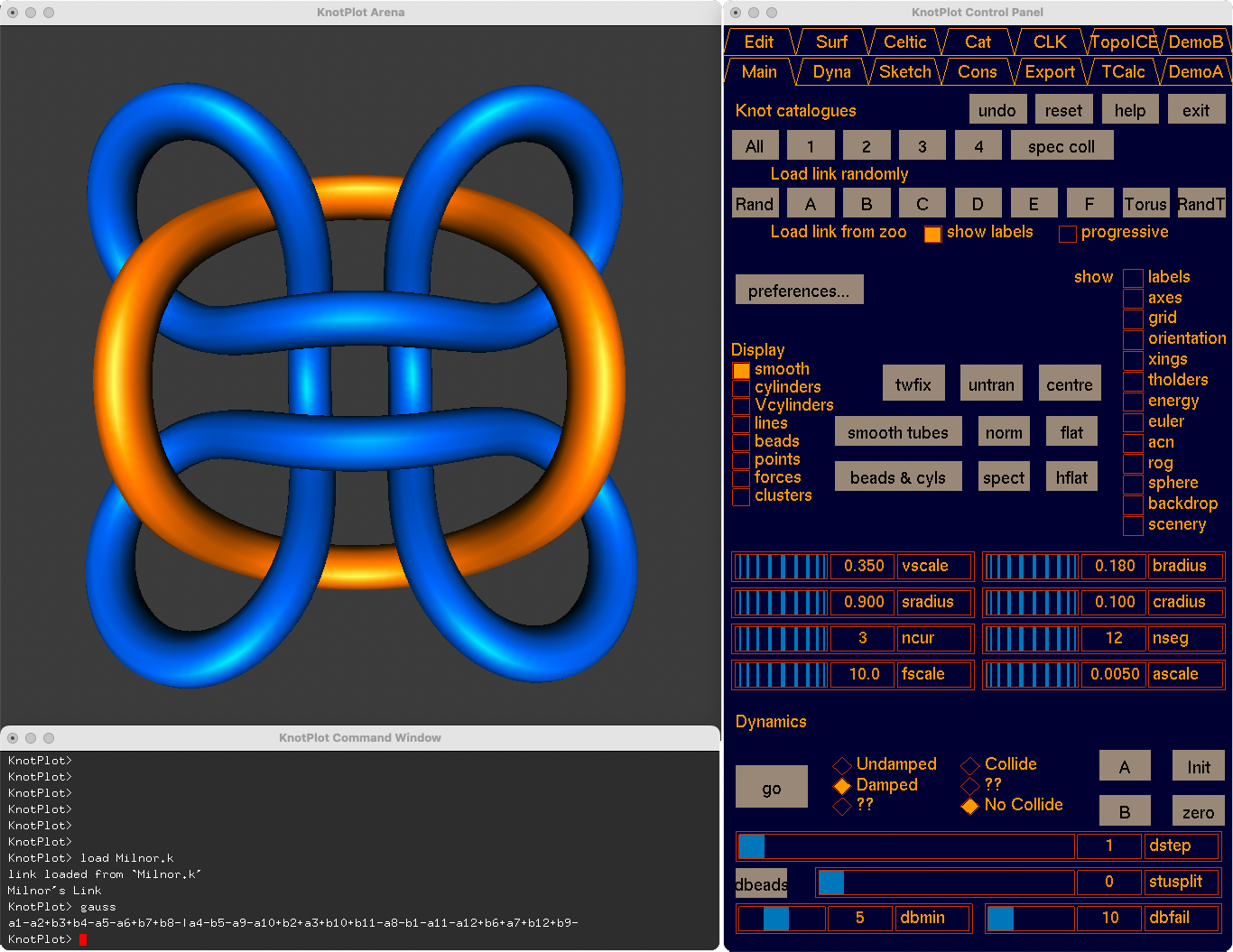
Figure 1. KnotPlot showing the Arena (upper left), Control Panel (right, set to the Main tab) and Command Window (bottom).

Figure 1 shows what KnotPlot looks like upon startup, after a knot of interest is loaded. KnotPlot opens three windows: KnotPlot Arena, KnotPlot Control Panel, and KnotPlot Command Window. The knot is displayed in the KnotPlot Arena where interactions using mouse and keyboard can be used. The KnotPlot Control Panel is used for many tasks. It is divided into a number of sub-panels that may be accessed using one of the 14 tabs at the top of the panel. In this document when we refer to a specific sub-panel we use the names shown, for example Main, Sketch, and DemoA. We discuss a few of these tabs in detail, please refer to Section 15 to see a brief description of the rest. The final option for interacting with KnotPlot is to use the KnotPlot Command Window. Here we see that that Milnor’s Link has been loaded and its extended Gauss code calculated by entering the commands load Milnor.k and gauss.

At the moment, the user interface looks identical on the various platforms, having been implemented in OpenGL [Gro22] and GLUT [Gro20]. This “Classic KnotPlot” does not use the native buttons, sliders, and menus of the platforms they are running on. For example, KnotPlot’s menus are accessed by right clicking on the Control Panel. While this universal look has a certain appeal, it may make KnotPlot more difficult to learn than it should be. Currently in beta testing is KnotPlot Redux, a cross-platform re-implementation of the user interface with native look and feel, with “Classic” mode available as a legacy option.

3. Loading and saving

We recommend that users create a project directory (folder) and start KnotPlot with that directory set as the working directory. If the working directory contains user’s knot files, they may be loaded with something like
        load myknot
where myknot is the name of knot file. If the file specified does not exist in the working directory, KnotPlot will search a list of directories to find the file. For more information on this, please refer to the path command.

KnotPlot comes with the entire Rolfsen Appendix C catalogue of knots and links [Rol76]. The KnotPlot names are formed in a simple way, for example
        load 3.1
loads the trefoil $3_{1}$ and
        load 9.2.14
the link $9^{2}_{14}$.

Most of the thousands of knots and links in KnotPlot’s various catalogues are stored in a compact binary format, but users can use a simple plain text format to load a configuration. This is one vertex per line with coordinates separated by spaces, and a blank line separating different components. For example the following represents the Hopf link $2^{2}_{1}$.
        0.10 -3.29 -0.49
        1.11 0.69 0.13
        -1.64 -0.27 0.26
        
        0.01 2.30 0.44
        -0.07 2.10 -0.87
        0.48 -1.55 0.53

Saving knots is done with the save command,
        save myknot
that will save to the working directory. KnotPlot supports saving in many different file formats. By default KnotPlot saves in its compact binary format. Appending a file extension to the file name will save in a different format, as in
        save something.txt
for simple plain text and
        save something.vect
for Geomview’s VECT format [Cen14].

4. Changing the view or embedding

The Arena shows the currently loaded knot using a virtual camera located at the starting position of $(0,0,8)$ with the centre of view being the origin. A viewing transformation is applied to the knot and may be modified using the following mouse or keyboard controls:

• Left click and drag rotates the view. You can also constrain the rotation using the keyboard. Press and hold one of x, y, or z before left clicking causes the rotation to be about one of those coordinate axes. These axes are in the coordinate space of the knot, which may be already rotated. If you want to rotate about axes fixed to the screen, press and hold i, j, or k instead (k goes into the screen). For precise control over rotation, use the rotate command.

• Middle click and drag to translate the view (or press the option/alt key (or ctrl key on some systems) and left click, and then drag).

• Right click and drag to scale the view (or press the shift key and left click, and then drag). The viewing scale can be set to an exact value using the vscale parameter.

These actions change only the view and not the actual embedding of the knot. Another command, about, does the complement, namely changes the actual embedding but not the view. The two may look exactly the same, for example compare rotate x 33 to about x 33, but they are not equivalent. The rotate demo in the Tutorials section on DemoA gives a good introduction to the differences between rotate and about. The rotate fix command is useful for transferring a view rotation to a rotation of the embedding.

5. Relaxing knots and links examples

Sometimes we might have a knot in a rather messy conformation and we would just like to get a nice picture of it. We can use the controls on Main to accomplish this. Try the following:

• If necessary click on the reset button to get KnotPlot into its starting configuration.

• Load a knot of interest, say the trefoil
          load 3.1
  or load it from the Knot Zoo using the A button on Main.

• Click on the beads & cyls button so that you can see edges and vertices of the knot.

• The dbeads button deletes edges in the knot without changing the knot type. Click on this button several times until nothing more can be deleted.

• Click the go button to start relaxing. That button will turn green to indicate relaxation is happening. You should see that the knot gets stuck.

• Now increase the value of stusplit using the slider. This allows any stuck edges to be split, in a way that maintains knot type. The knot should now look much more trefoilesque.

• Keep the relaxation going and get an even nicer trefoil by entering the split into the Command Window. This splits all the edges. You should see something looking much like what you started with.

• If you feel like trying another example, just keep the relaxation going and load a knot or link.

Here is a real-world example which also handles rotating the knot so that it can be loaded later from the given position. We will use a knot that comes from an experiment that RGS did to generate “compact” versions of knots fitting into a spherical cavity. Load one of these with
        load compact.k
and apply the method above, relaxing with a non-zero value of stusplit and repeatedly clicking on dbeads. When you have simplified it to your liking, stop the relaxation and click on the centre button. It will likely not be in an orientation showing a minimal crossing number. Try rotating it until it looks as minimal as possible. Now what we would like to do is to save the rotated version. We need to apply the viewing transform to change the coordinates of the knot. For this we use the rotate fix command and then save transformedknot. At this point, if you exit KnotPlot, restart KnotPlot, and then load transformedknot, you will see the view of the knot as you saved it (unless you scaled the knot using vscale).

Here is another example. This creates a link with many vertices and then simplifies the link.
        load 9.3.7
        (press the beads & cyls button)
        #2 split % splits each edge into two pieces, and does this twice
        fitto mindist 0.5 % scales so min dist between beads is 0.5
        go beadlimit 4000 % increase this value if there are many edges
        (press the go button, it will turn green)
        (press the dbeads button repeatedly)
        stusplit = 3
After a few seconds, the link should look similar to Figure 2. Press the go button again to stop the relaxation.

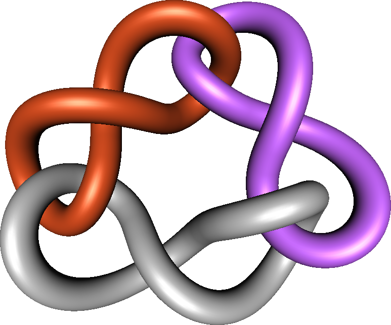
Figure 2. The link $9^{3}_{7}$.

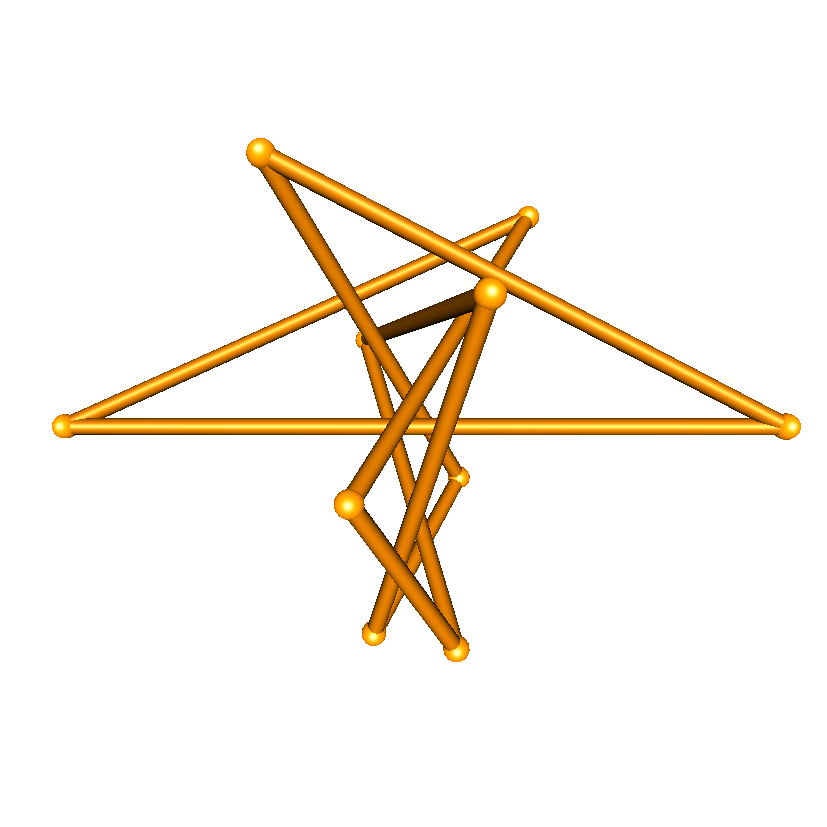
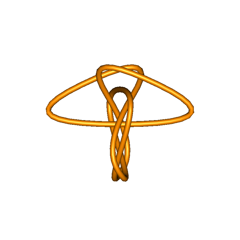
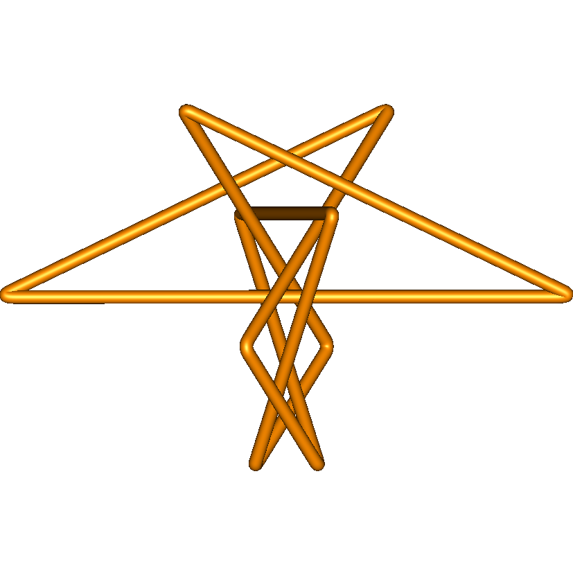
mode cb mode s mode s after splitting

Figure 3. Various renderings of minimal stick $10_{124}$.

6. Making pictures

Making full colour images of what is seen in the KnotPlot Arena can be made with the imgout command. The colour of different components may be changed in various ways using the colour command. Also, for publication purposes it is often desirable to have a white background rather than KnotPlot’s grey colour. Entering the sequence of commands
        load 9.3.7
        luxo
        background = white
        colour 0 grey
        colour 1 rgb:0.85/0.3/0.12
        colour 2 rgbi:199/102/255
        imgout 3complink
results in a file called 3complink.png, which is shown in Figure 2. The luxo command is just a shortcut to setting the values of ncur and nseg.

The next example is the kind of thing that we sometimes need to do to get a good illustration. Consider the knot on the left in Figure 3. This is a minimal stick representative of a knot found in RGS’s survey [Sch98], with an embedding that results from minimizing Simon’s minimum distance energy [Sim94]. It was then aligned using align axes. The knot exhibits a beautiful symmetry along all three axes but this is not completely evident in the left-hand figure because we are viewing in perspective. Suppose we want to show the symmetry and also draw the knot as just a polygon, without the little spheres showing the vertices. Switching to orthographic view with the command orthographic and to smooth mode with command mode s we get the middle figure, which may not be ideal. This is because the smooth tubes are drawn by using Bézier splines that interpolate the edges. The interpolation gives a correct look for knots only if the turning angle is not too large between edges. To get around this problem, we use the trick of splitting edges multiple times to get the view on the right. The commands that generated Figure 3 are below.
        luxo;background = white; mode cb; vscale = 0.8
        sradius = 0.12; cradius = 0.12
        load ms/10.124; about z -90
        display true;imgout polygonalLeft
        mode s;ncur = 11; ortho
        display true; imgout polygonalMiddle
        #4 split     % repeat split 4 times
        display true; imgout polygonalRight

Note that several commands can be typed on the same line using semicolons for separators and that % is the KnotPlot comment character (just like LaTeX). The command display true command is often used in scripts run from the command window to force a redraw of the frame buffer at that point. Otherwise the frame buffer does not get redrawn until the script finishes. If you type these commands in manually, you do not need display true. Note that these commands can be saved to a file, say myscript.kps, and then loaded through the command window via < myscript.kps. There is also a no graphics mode to KnotPlot which we discuss in Section 14.

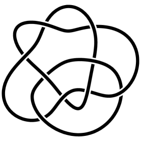
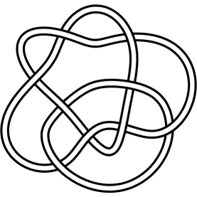
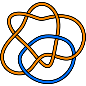
psmode = 40 psmode = 41 psmode = 45

Figure 4. The link $9^{2}_{37}$ in different styles.

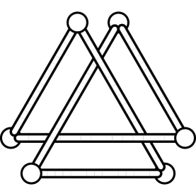
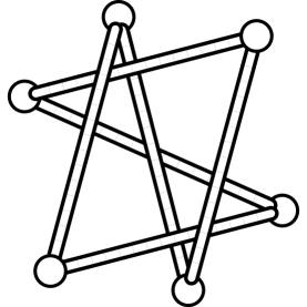
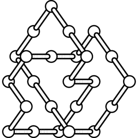
Minimal stick Equilateral minimal stick Cubic lattice

Figure 5. The trefoil in various minimal edge forms.

7. Making knot diagrams

KnotPlot can generate lightweight Encapsulated PostScript (EPS) files using something like
        psout filename
and there are wide variety of options. A simple example is shown in Figure 4, produced with the commands:
        mode s
        load 9.2.37
        psout knotLine
        psmode = 41 % default psmode mode is 40
        psout knotRolfsen
        psmode = 45
        psout knotOther

If KnotPlot is in piecewise linear mode (mode cb), the EPS figures look a little different. The following commands result in the images from Figure 5.
        mode cb; cradius = 0.16
        load ms/3.1; fitto avlength 3
        psout mstref
        load mseq/3.1
        fitto avlength 3; psout mseqtref
        load mscl/3.1; about x 45; about y 45; psout mscltref

RGS’s dissertation [Sch98] was heavily illustrated with EPS images of this sort. In addition to EPS images being lightweight, they also have the advantage as vector graphics that they may be scaled to arbitrarily large sizes without loosing their sharpness. To see the many flavours of PostScript output together with the KnotPlot scripts that created them visit the web page [Sch22e]. A few of these are shown in Figure 6 with the following links to the KnotPlot code that generated them:
https://knotplot.com/postscript/m/TangleE.html
https://knotplot.com/postscript/m/CelticH.html
https://knotplot.com/postscript/m/psm_eofill1.html
https://knotplot.com/postscript/m/3compBrunA.html
https://knotplot.com/postscript/m/tangle-holder-B.html
https://knotplot.com/postscript/m/combine-eofill-PL.html

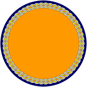
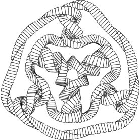
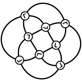
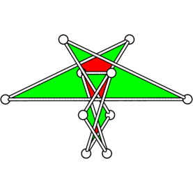
three string tangle Celtic knot checkerboard colouring Brunnian link tangle holder minimal stick $10_{124}$

Figure 6. Examples of Encapsulated PostScript diagrams

8. Creating knots and links

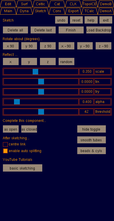
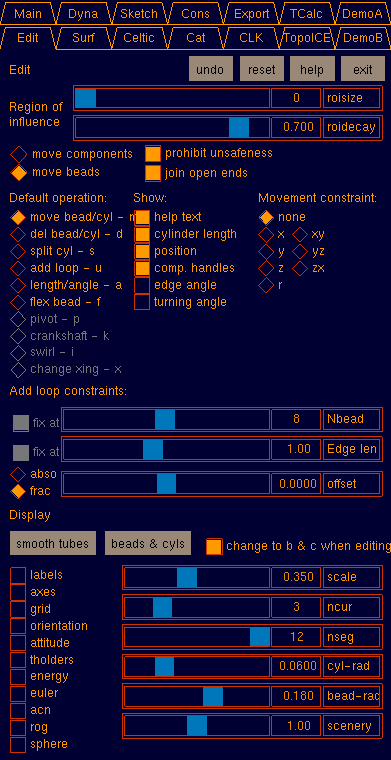
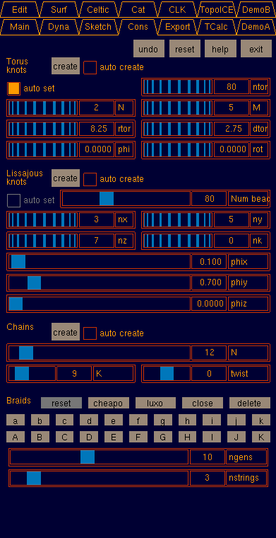
Sketch panel Edit panel Cons panel

Figure 7. Control panels for sketching, editing and constructing

8.1. Sketching

If you have some knot you would like to have coordinates for, you can use KnotPlot to sketch the entanglements. If you click the Sketch panel, shown in Figure 7, you can lay down points by left and right clicking. When you want to go over an existing strand, you use the right button. To go under, you use the left button. You will see that as you lay points down using the left and right buttons that the points will appear to be further away and closer to you, respectively. When you are done, click either as open or as closed button to complete the construction. You can also just hold down a button and drag around to lay down vertices at a reasonable pace. Adjust the threshold slider to control the spacing between beads when dragging. When you are finished sketching, exit sketching by going to another panel, for example Main.

When sketching, several keyboard operations can be useful, especially when sketching on a trackpad.

• Hold down the SHIFT key when left clicking to simulate a right click that goes over.

• Hold down the CONTROL key and left click and drag to translate the view.

• Hold down the OPTION/ALT key and left click and drag to scale the view. Click down at the location you wish to remain fixed when you scale.

8.2. Editing

If you want to move the vertices of a knot/link around, remove edges, remove vertices, etc., use the Edit panel. There are lots of choices here, but it is pretty straightforward to figure out. If prohibit unsafeness is checked (the default), KnotPlot will not let you leave the knot in an unsafe position (see Section 13) after any editing operation. Note that if this box is checked, it is still possible to change the knot type. KnotPlot does not check for unsafeness during the editing operation, only at the end. To change the knot type, the easier way is to leave the prohibit box checked, then increase roisize to a value near the top of the slider range. Then click and drag a bead or edge, pass a strand through another portion of the knot, and when things look clear release the button.

If you hover the mouse button over a bead or an edge, some information about that entity will be given. Exactly what information depends on what is selected in the Show: check box section on the Main panel. If you change something on the Edit panel, you might have to make sure the Arena window has mouse focus before you seen any changes. To do that, just left click the mouse anywhere on the background and things should work as expected.

The Default operation: list in the Control Panel shows what editing operations are available and is initially set to move beads/cylinders. If you want to delete one of those, select del bead/cyl and click on what you want gone. Again, remember to click on the background in the Arena to give that window mouse focus. It is actually not necessary to change the Default operation: to switch between operations. You can press and hold one of the shortcut characters m, d, s, u, a, or f to temporarily change the operation (the corresponding shortcuts are shown to the right of the operations).

You can constrain moving in various directions by changing the settings under the Movement constraint: list on the right. The letters indicate in which directions movement will not be allowed. For example, select xy to change only the $z$-coordinates.

One important thing to note is that, unlike when sketching, the editing mode allows you to rotate, scale, or translate the view in the normal KnotPlot mouse movements. Just remember when doing that, click down on an empty space, avoiding the knot, and then drag the mouse. It is for this and other reasons that Sketch panel will be removed in future versions of KnotPlot and its features added to the Edit panel.

Something fun to try:

1. Whilst on the Edit panel, enter the command   delete all

2. Enter the command   unknot

3. Click on the beads & cyls button in the Display section of Edit

4. Enter command   cut pieces 10

5. Increase roisize to at least 8

6. Click the none diamond in the Movement constraint: list

7. Click the join open ends box until it is selected

8. Enter the command   jitter 5

9. Enter the command   collision allow

10. Enter the command   until safe "ago 55"

You should now have a bunch of short strings that you can move around. If you bring two open ends within a certain distance of each other, you should see a green indicator showing a connection between the ends. Keep moving and the indicator will disappear. However, if you release the mouse button when the indicator is on, the two beads will be connected forming a new component. See if you can join all the ends to make a knot or a link. You might have to rotate and scale the view a few times. It might help to switch between move beads and move components.

8.3. Torus knots and links

The top part of the Cons panel shown in Figure 7 is used to create torus knots and links. To get a quick start, check the auto create box and start to adjust the N and M rollers. This will create an ($N$, $M$) torus knot/link with ntor edges, a meridional radius of rtor, and a longitudinal radius of dtor. You can also leave auto create unchecked, adjust all the rollers to desired values, and then click the create button to create the knot. As long as the auto set is checked, KnotPlot will pick an appropriate value for ntor. It can be interesting to uncheck this box, click the beads & cyls button on Main, and then set ntor so that the torus knot/link is undersampled. You can use the torus command to specify directly all values.

8.4. Lissajous knots

Lissajous knots [BHJS94] can be created with the next section down on Cons panel. Things work in a similar manner to the construction for torus knots, except the auto set is not available. Note that many embeddings created in this construction will be in an unsafe position (for a discussion of safety, see Section 13).

The Lissajous demo on DemoA can be quite a lot of fun. It chooses random values for the Lissajous knots and does not stop until it finds a safe embedding. When it does, you can click on the simplify knot button in the Arena. Often what looks like a high crossing number knot simplifies to an unknotted round circle.

8.5. Chains

This creates a chain with N components with K edges each that twist. More control can be had by using the chain command. To see what can be done with chains, run the chains demo on DemoA.

8.6. Braids

In this section, you set the number of generators and strings and then add positive or negative crossings one by one. Once again, the use of the braid command is much more flexible. To see what can be done with braids, run the braids demo on DemoA.

9. Useful commands

Below is a list of commands that are used with some frequency. We have included example numbers in these, but all of the numbers are specific to the context and what you are trying to do. The current version of KnotPlot has 357 commands, please consult the manual [Sch22b] to see what is not covered here.

about x 45 — This rotates the knot/link while keeping the axes fixed in place. This changes the coordinates of the knot/link. The $x$ is the axis you are spinning about, so you can use $y$ and $z$ too. See also rotate x 45.

acn — Computes the exact average crossing number (up to computer precision), i.e., the average of the number of crossings seen over all projections. This also computes the writhe, which is the average over all projections of the sum of the signed crossings.

ago 1000 — This runs the dynamics/relaxation for 1000 steps. While it is running, KnotPlot will not respond to any user actions. The ‘a’ in the command name stands for ‘atomic’, that is the command completes before anything else is allowed to happen. This should be used in place of go in scripts that are run in graphics mode. In non-graphics mode (see Section 14) the two commands are identical. See also go.

alias plpsout "psout $0" — Creates an alias. Aliases whose name begins with a $\sim$ are deleted upon a reset. Others, such as this one, will persist.

align axes — This puts the centre of mass at the origin and rotates the knot so that the principal moment of inertia axes are aligned with the $x$-, $y$-, and $z$-axes. This command tends to produce embeddings that minimize crossing numbers (in an orthographic projection to the $xy$-plane).

allocate 10000 — This allocates memory for knots/links with larger numbers of beads. Use with no argument to find the current amount allocated.

angle — This computes the minimum internal angle, maximum internal angle, ratio of maximum to minimum internal angle, and the average internal angle for each component.

angle turning — Toggles between computing the internal angle and the turning angle. The turning angle, which measures how much one edge turns relative to the one before it is equal to 180 minus the internal angle.

braid (aB)^3Ca — Creates a braid with the braid word $(\sigma_{1}\sigma_{2}^{-1})^{3}\sigma_{3}^{-1}\sigma_{1}$. The parentheses can be nested, so braid e(D(Bc^2)^3Ca)^2b would produce the braid $\sigma_{5}(\sigma_{4}^{-1}(\sigma_{2}^{-1}\sigma_{3}^{2})^{3}\sigma_{3}^{-1}\sigma_{1})^{2}\sigma_{2}$.

celtic box 4 6 2 — Creates a Celtic box of the given dimensions.

centre — Translates knot/link so that its axis-aligned rectangular bounding box is at the origin. The US spelling center is an alternative.

centre mass — Translates the knot/link so that its centre of mass is at the origin.

chain 10 — Creates a chain of unknots with 10 components.

cheapo — This command changes ncur and nseg to values lower than normally used. This command is useful when you want to reduce the rendering quality temporarily so that rotating and scaling the view is more responsive. The name borrowed from [Knu89, p. 150]. There is also a complementary luxo command.

close 4 — Closes the indicated component if the component is open. Use close all to close all components. See the open command.

collision allow — Turns off KnotPlot’s collision checking, allowing strand passages during relaxation. Use collision fast to go back to the default collision mode.

colour 0 red — This colours component 0 red. Use colour all red to set the colour to red for all components. The available colours are in the resource/colours.txt file within your KnotPlot installation directory. The colour names are essentially those from X11 [Wik22c] with a few additions. The names are case and space insensitive. You can also set the colour explicitly using RGB values, for example colour 2 rgb:.3/.5/1 where the values are in the range 0 to 1. For more complete information see [Sch22f]. The US spelling color may be used as an alternative. See also matrgb bead and matrgb knot.

conway 6,3,4 — Creates a pretzel link from the Conway notation [Con70]. Also prints out the tangle command string used to generate the link in the tangle calculator, in this case tangle 6r3r#4r#N

cut 27 — Deletes the edge starting at a given bead/vertex. Use show labels or check the box on Main to see the bead labels. Vertices are numbered starting at 0 and edge $n$ goes from vertex $n$ to vertex $(n+1)$ (modulo the number of edges, if the configuration is closed).

cut outside x 0 — Cut all edges that are entirely outside the plane $x=0$. To see all the options, run the cut demo in the Lua scripted demos section of DemoA (also view the Lua source).

cwd — This tells you the current working directory that KnotPlot is running from. If you save something, it goes into this directory. See also the path command.

delete 1 — If you have a link, this will delete component 1 (components are numbered starting at 0). Use undo if that was a mistake. See also keep 1.

delete downto 15 — Deletes vertices, while keeping the knot type fixed, to 15 vertices. Oftentimes it will not be able to get to that value, in which case it just stops. You can say delete downto 0 (equivalent to the dbeads button on DemoA) and that will do the best it can to get rid of extra vertices. Doing this periodically during relaxation and with the parameter stusplit set to a positive value is how the knots on the Split/delete demo on DemoA work. See the exercise in Section 5.

diagram 8 -10 -16 12 -14 6 2 -4 — Generates a configuration whose Dowker code is 8 -10 -16 12 -14 6 2 -4. Uses (with permission) the knot diagram engine by Morwen Thistlethwaite and Kenneth Stephenson modified slightly from the ‘draw’ routine in Knotscape [HT99].

display true — Forces a redisplay of the current state of the KnotPlot Arena. Useful mostly in scripts run in graphics mode when you want to ensure the display is correctly updated before creating a picture.

distance — Shows the minimum distance between non-adjacent edges. This is the value reviewed when you check on safety with the safe command. See Section 13.

dowker — KnotPlot computes Dowker codes [DT83] with this command as well as Extended Gauss Codes (EGCs) [GMGCL99] using the gauss command. By default, these commands compute their codes in a fixed projection that may not correspond to the view in the Arena. Please see the discussion of the dowker projection options on how to change modes so that the codes match the view. For a comprehensive introduction to crossing codes see the codes demo on DemoA.

dowker projection view — Set the Dowker projection mode to the view (as an orthographic projection) of the knot/link seen in the KnotPlot Arena. In this mode, the dowker and gauss commands will correspond to what is seen in the view window, and will change if you rotate the view. Same as gauss projection view.

dowker projection z — Set the Dowker projection mode to the $z$-projection (i.e., onto the $xy$-plane). In this mode, crossings are computing by orthographically projecting the edges to the $xy$ plane. The dowker and gauss commands will give codes that, if the knot has been rotated, do not correspond to what you see in the view window, especially if the knot is rotated. Alternately, one can do a rotate fix followed by dowker. Same as gauss projection z.

draw flat – Draws the knot/link so that the cylinders look like they are made out of rectangles.

draw hflat – Draws the knot/link so that the cylinders look like they are made out of long rectangles.

draw normal – Draws the knot/link in the default fashion.

draw spectrum – Draws the knot/link with rainbow colouring.

duplicate — Duplicates component 0. The duplicate will be directly on top of the original so you will not see both unless you move one of them. An example usage is to quickly create a composition of two $6.3$ knots:
        load 6.3
        shift maxx % shifts bead 0 to maximum x-position
        duplicate
        open all
        reflect x 1; translate 20 0 0 1
        join F0 F1; close all
        ago 333; centre

energy — Prints the knot energy according to the current energy model.

energy model — List the available energy models (there are more than a dozen to choose from). Change the energy model used with commands such as

• energy model MD — Simon’s minimum distance energy [Sim94]

• energy model symm — Buck and Orloff’s symmetric energy [BO95]

• energy model nbeads — Energy is the total number of beads in the knot. Can be useful when trying to reduce the number of vertices.

Consult the KnotPlot Manual for more information [Sch22b] on the different models.

exit — Same as the quit command. This command will quit KnotPlot if run from the Command Window. In scripts this causes the script to quit at that point in the script.

export mymodel — Exports a 3D polygonal mesh to the file mymodel.obj which is in Wavefront OBJ format [Wik22b].

fitto 10 — Multiplies the coordinates of the knot and centres it at the origin such that the maximum extent in the $x$, $y$ or $z$ directions is $\pm 10$. This command is useful for rescaling and centering the model so that it is in the viewing window.

fitto mindist 0.15 — This is like the normal fitto but it makes it so that the knot/link has a minimum distance of 0.15 between any two non-adjacent cylinders.

gauss — Works the same as the dowker command except that it computes the extended gauss code. How EGCs are computed is explained in Section 2.3 of the HOMFLY-PT chapter in this book.

gauss projection view — Same as dowker projection view.

gauss projection z — Same as dowker projection z.

go 1000 — This runs the dynamics/relaxation for 1000 steps. While it is running, KnotPlot will respond commands and user interactions. See also ago.

head 22 — Shows only the first 22 beads of the knot and hides the rest. Used on the demo braid warp on DemoA. Although the beads are hidden, they are really still there. Enter head off turn off hiding.

hide 1 — Hides component number 1. It is still there, but you will not be able to see it. The opposite is unhide 1.

hide all — Hides all of the components. They are still there, but you will not be able to see them. The opposite is unhide all.

homfly-pt – Computes the HOMFLY-PT polynomial. Alternative command names are homfly, homflypt and flypmoth. For references and a description of a stand-alone tool to compute these polynomials please refer to the HOMFLY-PT chapter in this book.

id – Attempts to identify the currently loaded knot or link using the homfly-pt command and KnotPlot’s built-in lookup table for HOMFLY-PT polynomials. This lookup table is limited in scope and not changeable by users. The HOMFLY-PT chapter has links to various knotting tools that have much more flexibility.

imgout tref — Saves the contents of the view window as the PNG file tref.png. If you want a JPEG instead, append .jpg to the file name, e.g., use the command imgout tref.jpg.

info — This tells the number of components, number of vertices/beads, and some other information. Use info s to get a short version of the same information.

jitter 0.1 — This moves each vertex by a random value $\leq 0.1$. If you have a lot of parallel edges (like in a lattice knot) and do something like try to find a crossing code, you will run into all sorts of problems (you will get division by 0 in some of the computations). You can use jitter to get out of that problem.

join L0 F1 — Join the last bead of component 0 to the first bead of component 1, creating a new component. Both components must be open.

keep 1 — If you have a link, this will delete all of the components but component 1. See also delete 1.

knot — Randomly choose a knot/link from the Rolfsen catalogue and load it. To choose a random link with 3 components use knot 3.

length — This computes the total arc length, minimum edge length, maximum edge length, ratio of maximum to minimum edge lengths, and the average edge length for each component.

line from 5 3 1 to -4 2 -7 — Create a line between two locations. You can omit the from and to.

lnknum — If you have a link, this will compute the linking number matrix, i.e., the linking number between each pair of components.

load file — Loads a knot/link file. See Section 3 for information on using this command.

load combine file — If you have one knot/link loaded and you want to load another knot/link as to form a union with what is there, you use load combine.

load sum file — This is used if you have a knot/link loaded and you want to do a composition with a new knot/link. You usually need to relax the knot/link after doing this. For links, you can specify which component of the currently loaded link that you connect sum with. For example, if you
     load 9.3.2
     load sum 3.1 0
you get something different than if you
     load 9.3.2
     load sum 3.1 1
For links, the component to compose with is set to a default value of 0.

lua run Brunnian — Run the given Lua program, in this case the Brunnian demo on DemoA.

luxo — This command changes ncur and nseg to values higher than normally used. This command is useful before exporting an image with imgout. The name borrowed from [Knu89, p. 150]. There is also a complementary cheapo command.

mass open — If you have an open knot, this anchors the first and last vertex so that they do not move during relaxation.

matrgb bead 0.1 0.4 0.8 — This changes the beads to the colour with RGB values of 0.1, 0.4, and 0.8. This affects all components.

matrgb knot 0.5 0.25 0.3 — This changes the cylinders to the colour with RGB values of 0.5, 0.25, and 0.3. This affects all components. If you just want to change the colour of one component, see colour.

mf myknot — Outputs the current knot as a Metafont [Knu89] program. Only works for 1-component knots.

mode cb — Puts KnotPlot in beads and cylinders mode. There is a button for this on the main panel, so you would probably only use this in a script.

mode s — Puts KnotPlot in smooth tubes mode. There is a button for this on the main panel, so you would probably only use this in a script.

nap $N$ — Pauses for $N$ seconds. You might use this if you are running a script to view knots, kind of like a slideshow, and you want it to pause a bit between each knot.

nbeads +5 — Adds 5 to the number of vertices. It does so by following a spline of the knot, so the new version typically has nicely distributed edge lengths. You can also subtract using nbeads -7, or specify a number exactly using nbeads 20. The latter is precarious because you can easily change knot type. You really only want to use this command if your knot/link is pretty smoothish looking to start. See also split and nbeads mult.

nbeads mult 3 — This is like nbeads but works as a multiplier. So this example triples the number of vertices. You really only want to use this command if your knot/link is pretty smoothish looking to start. See also nbeads and split.

open 3 — Opens component 3. Use open all to open all components. See the close command. This command opens a closed component by removing the edge between the 0${}^{\text{th}}$ bead and the last bead. If you want to open the component at another edge, see the shift command.

orthographic — Sets the view to an orthographic projection. In the default perspective view, objects that are further away look smaller. In the orthographic view, this is not the case.

panel set Cons — Set the Control Panel to the indicated tab. This could be used in an initialization script, for example, to get KnotPlot into a desired setup.

parameters — Lists all of the parameter values. If an argument is given, then KnotPlot will list all the parameters that start with that prefix. For example parameters ps will list all the parameters dealing with EPS output. You can do a
     parameters > pars.txt
and then open the pars.txt file to see all of the parameters.

path — Prints the read, write, and execute paths. See Section 12.

perspective — This switches the view to a perspective view, which is the default. In the projection view, things that are further away look smaller. In the orthographic view, this is not the case. The alternative is orthographic.

project random — Project the knot in a random direction. Changes the embedding, not the view.

psoption bbox square — Sets the bounding box option for psout. The are many other options that can be set. See the KnotPlot code on the PostScript examples page [Sch22e].

psout diagram — Generates an eps file called diagram.eps of a knot diagram version of the configuration you have loaded. See Section 7.

quit — The same as the exit command.

refine 3 — Refine the knot using Bézier interpolation by a given factor ($3$ times as many beads in this case). This command may change the knot type.

refine equilateral 1.02 — Refines the knot so it is approximately equilateral with the specified edge length. Use the length command to see how well it refined.

reflect x — This reflects the knot/link relative to the chosen $x$-axis. You can also use $y$ or $z$. In other words, it flips the signs of the $x$ (or $y$ or $z$) coordinates. Any one of these will create the mirror image of the given knot/link. You can combine reflections, as in reflect yx or reflect in a randomly chosen direction reflect r. If you want to reflect a single component of a link, specify the component number reflect z 2.

reset — This resets the viewing transform, the display mode, and other things, keeping the knot/link currently loaded.

reset all — Resets KnotPlot to its startup state. Also see the gentler reset command.

revbeads 1 — This reverses the orientation on component 1. Without any arguments revbeads reverses all the components. If you click on the Labels box on the right side of DemoA, you can see the vertex numbering change when you do this.

rog — Computes the radius of gyration.

rotate x 45 — This rotates the camera while keeping the knot/link the axes fixed in place. This does not change the coordinates of the knot/link. You need to use rotate fix after this, or after rotating the knot/link with the mouse, if you want to change the coordinates. The $x$ is the axis you are spinning about, so you can use $y$ and $z$ too. See also about x 45.

rotate fix — If you have rotated the view using rotate or using the mouse, the coordinates of the actual knot/link will not have changed, just the viewing transformation. This command changes the coordinates so that the view you are seeing is lined up so that you are looking down the $z$-axis. A useful command if have a nice view of something you created and want to adjust the embedding so that when you save your knot and load it back into KnotPlot, you do not have to any rotating to get back to that view.

rotate unit — Resets any rotations you have done with the mouse or with the rotate command.

safe — This tells you whether the knot/link is in a KnotPlot safe configuration. See Section 13 for details.

save file — Saves a knot/link file. See Section 3 for information on using this command.

scale 2 — This multiplies all of the vertex coordinates by 2.

scale 2 4 0.8 — This non-proportionally scales the knot/link coordinates by a factor of 2 in the $x$-direction, 4 in the $y$-direction and 0.8 in the $z$-direction. This command will not change the knot type.

shift 5 — This shifts the labels on the vertices by 5. So, for example, if you want some other vertex to be the $0^{th}$ vertex, you can use a shift to make that happen.

show orientation — Shows orientation arrows on the components. This command has many other options in addition to orientation (see the show check boxes on the Main panel).

split — This adds a vertex half way into each edge, doubling the number of vertices. See also nbeads and nbeads mult.

swap 2 4 — Swaps the numbering of the components indicated. Use swap random to swap all components randomly.

tangle 21*r2r#2r#N — Create the link $7^{2}_{5}$ using the tangle calculator. Use the conway command to see how the Conway notation gets parsed into tangle calculator commands. Also try the interactive tangle calculator on the TCalc panel.

tfunction 2.3 knot — Queue an arbitrary command to be executed in a given number of seconds.

thickness — This computes some sense of thickness. It is not equivalent to EJR’s definition of knot thickness [Raw97, Raw98, Raw03].

timer start gumby — Start a named timer. The name is arbitrary and you can have as many timers as you wish. Check the timer at some point in the future with timer check gumby.

torus 3 5 50 11 2 — Creates a (3,5) torus knot with 50 edges where the longitudinal radius is 11 and the meridional radius is 2. You can skip last three parameters and KnotPlot defaults to the current value of the parameters N-torus, R-torus, and d-torus.

translate 5 8 3 — This translates the knot by 5 in the $x$ direction, 8 in the $y$-direction, and 3 in the $z$-direction. Changes the embedding, not the viewing transform in a similar manner to about. To un-transform a translation, do a undo command immediately after the unwanted transformation. Note, translations are not undone by untran, which resets the viewing transform.

translate to 5 3 7 — This translates the knot so that the 0th vertex is at (5,3,7). You can use shift to set a different vertex as the 0th vertex if you want to move a different vertex to a particular point in space.

twfix — Sets the value of twist (found on the Surf panel) to the value required so that the cross sections of the smooth tubes align at the beginning and end. For example, to see what this does, type
     load 8.18
     draw flat
     nseg = 3
You will find an unsightly twist in the smooth tube. Entering twfix makes this disappear.

undo — This undoes any changes just made to the knot.

unhide 1 — Unhides component number 1 if it is hidden. Now you can see it. The opposite is hide 1.

unhide all — Unhides all of the components. Now you can see all of the components. The opposite is hide all.

unknot 50 5 — Creates a regular 50-gon on a circle of radius 5. If the radius is omitted, it defaults to the current value of N-torus.

untran — Resets the viewing transform to the unrotated/untranslated one.

version — Use this command to find out the version, build number, and compile date of the KnotPlot you are running. Also shows you where the KnotPlot home directory is.

xing — This tells you the number of crossings seen looking down the $z$-axis. If you have rotated the knot, it might not give you the number you are seeing. If you do a
     rotate fix
and then
     xing
then you will see the number of crossings from the view you are looking at (at least the orthographic version of it).

10. Parameter values

The values in the sliders and rollers are parameters that can be set directly via a command like
     sradius = 1
for example. This is useful to set a parameter to an exact value, which might be difficult using the slider/roller. The majority of parameters in KnotPlot do not have a slider/roller associated with them. See the parameters command description.

Some of the most frequently used parameters are the following:

background — Used to change the background colour. Typically, you do a background = white. See the colour command for more detail.

bradius — The radius of the sphere representing the beads (vertices). Has a roller on Main.

cradius — This controls the radius of the cylinders in the knot in beads and cylinders mode. Has a roller on Main.

dbmin — The minimum number of beads that delete downto will delete to. Has a slider on Main.

dstep — The number of relaxation steps between each redisplay. Defaults to 1. Increasing the value helps to speed up relaxations if the rendering time is significant.

duc = true — This is good to put at the start of any scripts that are used in production runs. It will cause KnotPlot to have a panic exit if it “complains” about anything. A complaint is made whenever there is a major error, such as a typo causing an unknown command error. They are prefaced with the text ***. The name comes from “die upon complaining”.

hstart , hincr , satur and value — Controls the hue, saturation, and value (HSV) of knots and links in the default colouring mode (auto). To get a feel for how these work, go to the Surf panel and enter the following commands:
        reset all
        chain 18
and then play with the top four sliders on Surf.

ncur — KnotPlot draws the smooth tubes based on a Bézier spline interpolation of the polygonal knot. This is the number of interpolation points per edge. Increase to 10 or more for a smoother look. Run the bezier demo on DemoB for an interactive experience. Has a roller on Main.

nseg — The number of subdivisions in the meridional direction for both the smooth tubes and the cylinder. Load a knot/link and then try the following commands to get a neat extruded triangle look:
        mode s
        nseg = 3
        draw hflat
        twfix
Has a roller on Main.

N-torus — The default number of beads used if that parameter is omitted for commands such as torus and unknot.

pserase — This controls the amount of white space near crossings in a knot diagram when you use psout. See Section 7.

psmode — This controls the output mode when using psout. There are lots of different values. See Section 7.

sradius — This controls the radius of the tube about the knot smooth tubes mode. Has a roller on Main.

stusplit — Sets how many relaxation steps are done between checking for stuck edges. A value of 0 turns off checking. Has a slider on Main.

vscale — The scale component of the viewing transform. Has a roller on Main. Note that this affects the view of the knot, but not the coordinates.

11. User interface

This section is about buttons, boxes, and rollers in the Control Panel in the Main tab. Below is a description about what most of the controls on Main do.

Everything on this panel can also be done using commands (described in Section 9) or by changing parameter values directly (described in Section 10).

undo — undoes last action, equivalent to the command undo

reset — resets most of KnotPlot’s state to the startup values but keeps the currently loaded knot, equivalent to the reset command

help – a brief description of the options in the selected tab

exit – quits KnotPlot, equivalent to the commands quit and exit

All – loads a randomly chosen prime knot or link from the Rolfsen catalogue
1 – same as above but restrict to knots (i.e., 1-component links)
2 – restrict to 2-component links
3 – restrict to 3-component links
4 – restrict to 4-component links

Knot / Link Zoos

Rand – Randomly chosen from the Rolfsen catalogue
A – The knots $0_{1}$ to $9_{28}$
B – $9_{29}$ through $10_{43}$
C – $10_{43}$ through $10_{107}$
D – $10_{108}$ through $10_{165}$ and a few prime 2-component links
E – loads most of the prime 2-component links
F – loads prime 2, 3, and 4-component links and one 5-component link
Torus – loads torus knots and links in order of crossing number; you can keep clicking it to get the next set of more complicated ones
RandT – loads randomly selected torus knots and links

Boxes under “Display” on the left

These check boxes toggle various display modes: smooth are the smooth tubes (interpolated from the cylinders/edges), cylinders are centred on the edges of the knot, and Vcylinders are like cylinders but they meet up more nicely. Edges can also be drawn as lines. The vertices of the knot can be drawn as beads (spheres centred on the vertices) or points. By selecting forces you will see force vectors showing where the knot is moving if you press the go button. See the Section 13 for more information about the dynamics.

In the centre

twfix, untran, and centre are equivalent to the commands of the same name

smooth tubes is equivalent to the command mode s

norm is equivalent to the command draw normal

beads & cyls is equivalent to the command mode cb

spect is equivalent to the command draw spectrum

flat is equivalent to the command draw flat

hflat is equivalent to the command draw hflat

Boxes on the right

labels will let you see the vertex, edge numbers, and component numbers. The $n^{th}$ edge is the one starting at vertex $n$. Vertex and edge counting start at 0.

axes lets you see the $x$, $y$, and $z$-axes

grid lets you see the $xy$ plane

orientation puts some arrows on the knot so that you can see the orientation

backdrop gives you a coloured background

Rollers

vscale modifies the viewing transform, short for viewing scale

cradius controls the cylinder radius in beads and cylinders mode

bradius controls the bead radius, i.e., the vertex sphere radius, in beads and cylinders mode

sradius controls the thickness of the tube in smooth tubes mode

ncur and nseg control the level of refinement for the graphics of the cylinders (nseg only) and smooth tubes (both).

Dynamics

Dynamics is a mini version of what you see under the Dyna tab. For more detailed control of the dynamics, see Section 13.

Init is the normal dynamics. A, B, and zero are some other pre-loaded dynamics settings that change the relaxation. You can play around with these, but generally you will not want/need to change these dynamics settings. The Collide box allows the knot type to change, which can be useful in some situations. Relaxation mode undamped should generally be used only when the parameter velfo (velocity damping, available under the Dyna tab) is turned on.

dstep is how many dynamics steps happen between displaying the new configuration. If you increase this, things will move faster because the computer does not need to spend so much time rendering the image.

stusplit and dbeads are usually used in conjunction to simplify complex or awkward configurations. See the exercise in Section 5 for an example of how to use these features.

12. KnotPlot distribution

12.1. Where the files are

In a similar manner to the command path inside a terminal shell, KnotPlot has a read, write, and execute path. Users can see what these are or change the paths using the path command. On a typical Linux installation, this would print something like

Current execute path:
   .
   /usr/share/knotplot/resource/linux
   /usr/share/knotplot/resource/generic
Current write path:
   .
Current read path:
   .
   /usr/share/knotplot/basic
   /usr/share/knotplot/special
   /usr/share/knotplot/demos

We can see that the current working directory (represented by .) is first in all the paths, so a load command will first look in the that directory for a knot file. If it is not found, then the basic, special, and demos directories are searched in that order. These directories, as well as resource, are located under the KnotPlot home directory and have the following function:

basic — Contains the Rolfsen catalogue plus a few composite knots.

demos — The KnotPlot script files that implement the demos on DemoA and DemoB are found here. Two of these files, DemoA.kps and DemoB.kps define which buttons appear on the demo tabs. Because the working directory is first in the read path, it is possible to customize the DemoA or DemoB panels by creating a local copy of one of these files in that directory. To create a starter file, right click on the Control Panel and select one of the menu entries as shown in Figure 8. The .kps files are just plain text and can be edited with any text editor.

resource — A varied collection of resources that KnotPlot relies upon. The definition for the named colours that the colour command recognizes is in the colours.txt file. The src subdirectory contains example C++ code to read and write KnotPlot’s native binary format [Sch10] for knots/links.

special — A “Special Collection” of many knots and links of interest in knot theory and in popular culture. To load a randomly chosen member of this collection, click on the spec coll button on Main or enter the command knot special.

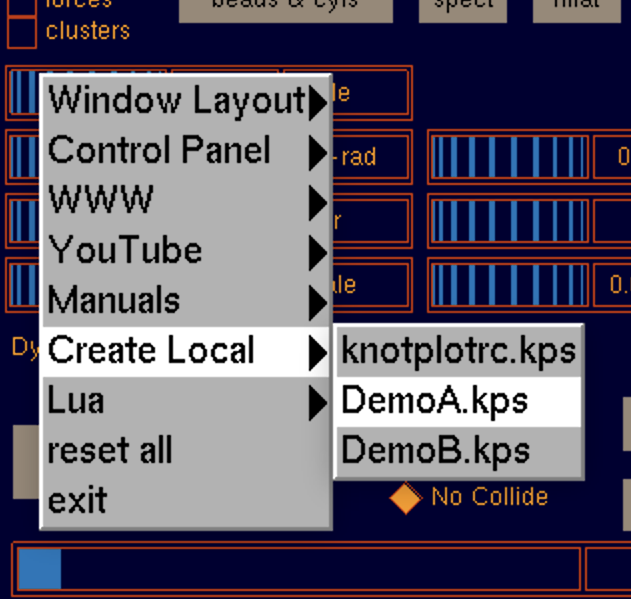
Figure 8. Creating a starter DemoA.kps file.

12.2. Various catalogues

As mentioned in Section 3 KnotPlot comes with the Rolfsen catalogue in versions that are similar to Appendix C of Rolfsen’s book [Rol76] (they are flipped vertically). This catalogue is also available in several other versions, whose knots can be loaded by prepending a subdirectory name (one of ms, mseq, or mscl) to the knot name.

Minimal stick — Finding minimal stick representatives for knots is work that was pioneered by Richard Randell [Ran94]. RGS extended the known values to all prime knot types up to 10 crossings [Sch98].
        load ms/10.124

Minimal stick equilateral — Modifying techniques used in the work mentioned above, the authors [RS02] found proposed equilateral minimal stick representatives.
        load mseq/8.19

Minimal step cubic lattice — Extending the work by Diao [Dia93], RGS found minimal step candidates for all knots and links in the Rolfsen catalogue. This work, in addition to some interesting theoretical results, was published in [SIA⁺09].
        load mscl/10.123

The minimal edge versions of the trefoil are shown in Figure 5.

In addition, KnotPlot includes the census of the simplest hyperbolic knots by Callahan, Dean, and Weeks [CDW99]. This study ranks the knots arranged according to the complexity of their complements, rather than by crossing number as is usually done. Load the simplest knot in this catalogue with
        load census/k2.1
and you will see that it is the Figure-8 knot. The 3D versions of these knots were created by RGS in collaboration with the authors of the study.

12.3. Knots and links in Virtual Reality (VR)

If you happen to be away from KnotPlot, you can still view the knots mentioned in the subsection above as well as knots and links from the Knot Zoo by going to one of the web pages
https://knotplot.com/zoo/
https://knotplot.com/stick-numbers
https://knotplot.com/hyper/

On any browser on a computer or mobile device, you will see a 3D model that you can rotate and scale. However, if you happen to own a VR headset, you will enter into a space where you can walk around your chosen knot or link and interact with it in other ways.

These pages are a work-in-progress and will be enhanced over time. Also, example JavaScript code will be supplied in case you want to showcase your own creations in ordinary 3D or in immersive VR.

13. Advanced dynamics

KnotPlot uses a simple force-based dynamical model to relax and simplify knots. This model is designed to maintain knot type during relaxation. An important concept in the model is the notion of safeness. A polygonal knot is said to be in a safe position if no two non-adjacent edges are closer than a certain threshold distance called close. During relaxation vertices are moved one at a time a distance not exceeding max-dir. Part of the condition for maintaining knot type is that max-dir be strictly less than close. These parameters can be changed on the Dyna tab of the KnotPlot Control Panel or by setting them directly: close = 0.12 and max-dir = 0.1. You can check to see if your knot is in a safe position using the safe command. A knot in an unsafe position can usually be made safe by simply scaling it with the scale command or to use the fitto mindist command with a value larger than max-dir. For a detailed discussion of KnotPlot’s dynamical model and a simple proof that it maintains knot type during relaxation see Section 7.1 of RGS’s dissertation [Sch98].

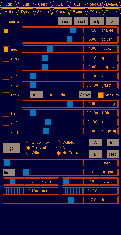
Figure 9. The Dyna panel showing options for the dynamics

Changes to the dynamical model can be done through the use of commands and parameters or by changing settings on the Dyna panel. Figure 9 shows the settings upon startup. By default only the elec force (repulsive) and mech force (attractive) are turned on. Forces may be toggled on/off using the check boxes or by typing a command, for example
        velfo = on
Each of the forces also has a corresponding strength (on the right hand side of the panel) that can be set using the sliders or by typing a command.
        velmag = 0.2
At the bottom of this panel are other options, for example checking the (inappropriately-named) Collide radio button allows edges of the knot to pass through each other, thereby allowing the knot type to change.

As mentioned before, the dbeads button deletes as many edges as it can without changing the knot type. This is usually done in conjunction with allowing edges to split if pairs of edges are in a stuck situation. Increasing the value of stusplit to something non-zero will cause KnotPlot to check every few relaxation steps on whether there are any stuck edges (according to the value of the slider). For a demonstration of the effectiveness of using this technique in simplifying complex knots, try the Split/delete demo on the DemoA control panel. This demo is essentially equivalent to the user randomly clicking dbeads every so often.

Here is a description of the various forces that are available. All these forces are applied to the beads/vertices, not the edges.

elec — A repulsive force similar to an electric field but generally with a higher power in the falloff compared to the $1/r^{2}$ Coulomb force. You can set that power as well as the magnitude of the charge. This force is applied to all pairs of beads that are not connected by an edge.

mech — Attractive force similar to a spring but non-linear. Change the strength of this force using hooke. The force is applied to beads that are connected by an edge. This allows the user to keep some control of the ratio of longest to shortest edge lengths.

amech — An alternative to mech that attempts to get the edges to a preferred length set by the parameter spring.

velfo — A velocity damping force similar to wind resistance. Only active if the force model is Undamped.

grav — Gravity force. Try the knot drop and snakes 2 demos on DemoB.

anch — Set some fixed anchor points that are attached to each bead. The force behaves in a similar way to the mech force. This is good to use if you just want KnotPlot to refine an embedding you have made so that it looks a bit smoother, but not change the configuration too much. Relaxing a sketched knot using anchors will not generally change the crossing number.

therm — A “thermal” force that applies a random nudge to each bead at every iteration step.

tanf — Force applied in a tangential direction to each bead in the direction of its associated edge. See the snakes 2 demo where a bunch of “snakes” are dropped onto a plane and they attempt to reptate out of a trap. Try also the demos swim and dolphins. These demos are on DemoB.

drag — Enabling this force allows you to click down on a bead and drag it to a new location. Try this in in beads and cylinders mode and run the demo mentioned below.

A good way to get a sense of the various force options is to play with the Forces, Anchors, and FreeDrag demos on DemoA.

14. Scripting with and running without graphics

Scripting can be used with the Command Window or run in no graphics mode. For example, suppose you have a bunch of KnotPlot commands collected in a plain text file script.kps. You can get KnotPlot to execute this script by entering
     <script.kps
into the Command Window.

For experiments, KnotPlot can be run in non-graphics mode. To do this, enter
     knotplot -nog < script.kps
into a terminal window. As was mentioned earlier, the command ago (used to run energy dynamics) is an “atomic go”, it completes what it is doing before letting anything else happen. In non-graphics mode, go is interpreted as ago. In this mode, KnotPlot will not open any windows and commands that require a frame buffer (such as image-producing commands like imgout) will do nothing. However, psout will work the same as it does in graphics mode.

Through most of KnotPlot’s history, scripts have been written in the commands described in this document (and many others). These native commands can do many things, but they are not a general purpose programming language. In early 2022 such a language, Lua [Wik22a, ICdF22], was embedded into KnotPlot. This addition has simplified and greatly enhanced the process of scripting.

15. Tabs

We have only discussed a few of the 14 Control Panel tabs in any detail (Main, Cons, Sketch, Edit, and Dyna). Here is a brief description of the others. When you go to any of these tabs, be sure to click on the help button at the top of the panel. The help is specific to the tab you are on.

Surf – Change surface properties of knots and links (colouring mode, various radii). All of these can be changed using commands or parameters. Camera parameters may also be set here such as field of view (FOV) and the distance the camera is from the origin. If these sliders are ghosted out, click on the Perspective radio button. Try setting vcn to a non-zero value and then adjust vcA and vcphi.

Celtic — Create Celtic knots. Quick start: click on one of the 20 preset configurations at the bottom of the panel, for example josephine. Then click on the diagram button at the top. This will show you the interlace pattern. Next click on the copy to arena button. Try the celtic demo on DemoA.

Cat — Most interesting here is a catalogue of 1736 decorative knots and links with $C_{n}$ and $D_{n}$ symmetry for $3\leq n\leq 8$.

Export — The buttons on this panel are intended as demos only. Use the relevant commands for actual work (psout, imgout, and export). Important: click on the how to set up a project folder (YouTube) button on the bottom.

CLK — Knot and links on the simple cubic lattice. This panel uses RGS’s implementation of the BFACF algorithm [vRW91].

TCalc — An interactive tangle calculator. The tangle command can be used to send a string of operations to the tangle calculator.

TopoICE — This is the Topological Interactive Construction Engine [DSS08, DS06]. It is an interface to software written by Isabel Darcy and uses the tangle calculator extensively. This tool is related to site-specific recombination in DNA. Manuals can be found on the KnotPlot download page [Sch22g].

DemoA, DemoB — A collection of demos that may be interesting or even fun. Briefly, the demos on DemoA that most useful for learning what the dynamics can do are Split/delete and Forces. For a complete description, please see the PDF document (ever evolving) A Rough Guide to the KnotPlot Demos that is located in the KnotPlot installation folder or can be downloaded from [Sch22a].

There are several more tabs that can only be accessed by right clicking on the Control Panel and selecting the Control Panel submenu. Perhaps the most interesting of these is the 4D tab that allows users to create 4D knots from 3D knots. We will leave that for you to explore.

16. Commands listed by activity

In this section, We have grouped the commands by certain activities that you might be trying to do. The list of activities is below, then followed by the pertinent commands (whose descriptions are in Section 9).

16.1. Changing the knot/link coordinates

• about

• nbeads

• nbeads mult

• reflect

• revbeads

• rotate fix

• scale

• shift

• split

• translate

• translate to

16.2. Isolating components in links

• delete

• hide

• hide all

• keep

• unhide

• unhide all

16.3. Combining multiple knots/links

• load combine

• load sum

16.4. Making a knot/link look nice

• align axes

• centre

• centre mass

• delete downto

• fitto

• fitto mindist

• nbeads

• nbeads mult

• rotate

• rotate unit

16.5. Making pictures

• background

• bradius

• colour

• cradius

• display true

• draw flat

• draw hflat

• draw normal

• draw spectrum

• imgout

• luxo

• matrgb bead

• matrgb knot

• mode cb

• mode s

• orthographic

• perspective

• psout

• rotate

• twfix

• pserase

• psmode

• psoption

16.6. Relaxing a knot/link

• ago

• delete downto

• go

• mass open

• stusplit

16.7. Technical issues and information

• allocate

• cwd

• duc

• info

• jitter

• parameters

• quit

• reset

• resetall

• undo

• untran

16.8. Knot/Link configuration measurements

• acn

• angle

• energy

• length

• lnknum

• rog

• thickness

16.9. Scripting

• ago

• lua

• mode cb

• mode s

• nap

16.10. Crossing information

• diagram

• dowker

• gauss

• xing

16.11. Special knot constructions

• braid

• torus

• unknot

16.12. Safety

• distance

• fitto mindist

• safe

16.13. File input/output

• load

• load combine

• load sum

• save

References

- [AJS+15] Javier Arsuaga, Reyka Jayasinghe, Robert Scharein, Mark Segal, Robert Stolz, and Mariel Vazquez. Current theoretical models fail to predict the topological complexity of the human genome. Frontiers in Molecular Biosciences, 2, 2015.
- [BHJS94] M. G. V. Bogle, J. E. Hearst, V. F. R. Jones, and L. Stoilov. Lissajous knots. Journal of Knot Theory and Its Ramifications, 3(2):121–140, 1994.
- [BO95] G. Buck and J. Orloff. A simple energy function for knots. Topology and its Applications, 61:205–214, 1995.
- [CDW99] Patrick J. Callahan, John C. Dean, and Jeffrey R. Weeks. The simplest hyperbolic knots. Journal of Knot Theory and Its Ramifications, 8(3):279–297, 1999.
- [Cen14] The Geometry Center. Geomview manual. http://www.geomview.org/docs/html/VECT.html, 2014.
- [Con70] J. H. Conway. An enumeration of knots and links, and some of their algebraic properties. In John Leech, editor, Computational Problems in Abstract Algebra, pages 329–358, 1970.
- [Dia93] Y. Diao. Minimal knotted polygons on the cubic lattice. Journal of Knot Theory and Its Ramifications, 2:413–425, 1993.
- [DS06] Isabel K. Darcy and Robert G. Scharein. TopoICE-R: 3D visualization modeling the topology of DNA recombination. Bioinformatics, 22(14):1790–1791, 05 2006.
- [DSS08] I. K. Darcy, R. G. Scharein, and A. Stasiak. 3D visualization software to analyze topological outcomes of topoisomerase reactions. Nucleic Acids Research, 36(11):3515–3521, 04 2008.
- [DT83] C. H. Dowker and Morwen B. Thistlethwaite. Classification of knot projections. Topology and its Applications, 16:19–31, 1983.
- [GMGCL99] G. Gouesbet, S. Meunier-Guttin-Cluzel, and C. Letellier. Computer evaluation of HOMFLY polynomials by using gauss codes, with a skein-template algorithm. Appl. Math. Comput., 105(2–3):271–289, 1999.
- [Gro20] Khronos Group. GLUT – The OpenGL Utility Toolkit. https://www.opengl.org/resources/libraries/glut/glut_downloads.php#1, 2020.
- [Gro22] Khronos Group. OpenGL – The Industry’s Foundation for High Performance Graphics. http://opengl.org, 2022.
- [HT99] Jim Hoste and Morwen Thistlethwaite. Knotscape. http://www.math.utk.edu/morwen/knotscape.html, 1999.
- [ICdF22] Roberto Ierusalimschy, Waldemar Celes, and Luiz Henrique de Figueiredo. The Programming Language Lua. https://www.lua.org, 2022.
- [ISD+12] K Ishihara, R Scharein, Y Diao, J Arsuaga, M Vazquez, and K Shimokawa. Bounds for the minimum step number of knots confined to slabs in the simple cubic lattice. Journal of Physics A: Mathematical and Theoretical, 45(6):065003, jan 2012.
- [Knu89] Donald E. Knuth. The Metafont Book. Addison-Wesley Longman Publishing Co., Inc., USA, 1989.
- [Ran94] Richard Randell. An elementary invariant of knots. Journal of Knot Theory and Its Ramifications, 3(3):279–286, 1994.
- [Raw97] Eric J. Rawdon. The Thickness of Polygonal Knots. PhD thesis, University of Iowa, 1997.
- [Raw98] Eric J. Rawdon. Approximating the thickness of a knot. In Ideal knots, pages 143–150. World Sci. Publishing, Singapore, 1998.
- [Raw03] Eric J. Rawdon. Can computers discover ideal knots? Experiment. Math., 12(3):287–302, 2003.
- [Rol76] Dale Rolfsen. Knots and Links. Publish or Perish, Inc., 1976.
- [RS02] Eric J. Rawdon and Robert G. Scharein. Upper bounds for equilateral stick numbers. Contemporary Mathematics, 304:55–75, 2002.
- [Sch98] Robert Glenn Scharein. Interactive topological drawing. PhD thesis, Department of Computer Science, University of British Columbia, 1998.
- [Sch10] Rob Scharein. KnotPlot File Formats. https://knotplot.com/manual/FileFormats.html, 2010.
- [Sch22a] Rob Scharein. A Rough Guide to the KnotPlot Demos. https://knotplot.com/manual/guide, 2022.
- [Sch22b] Rob Scharein. KnotPlot — A Program for Viewing Mathematical Knots. https://knotplot.com/manual/KPman.pdf, 2022.
- [Sch22c] Rob Scharein. KnotPlot Download Site. https://knotplot.com/download, 2022.
- [Sch22d] Rob Scharein. KnotPlot Manual. https://knotplot.com/manual, 2022.
- [Sch22e] Rob Scharein. KnotPlot PostScript / PDF Examples. https://knotplot.com/postscript, 2022.
- [Sch22f] Rob Scharein. Setting Colour in KnotPlot. https://knotplot.com/manual/colour, 2022.
- [Sch22g] Robert G. Scharein. KnotPlot Download Site. https://knotplot.com/download, 2022.
- [SIA+09] R Scharein, K Ishihara, J Arsuaga, Y Diao, K Shimokawa, and M Vazquez. Bounds for the minimum step number of knots in the simple cubic lattice. Journal of Physics A: Mathematical and Theoretical, 42(47):475006, November 2009.
- [Sim94] Jonathan K. Simon. Energy functions for polygonal knots. Journal of Knot Theory and Its Ramifications, 3(3):299–320, 1994.
- [vRW91] E. J. van Rensburg and S. G. Whittington. The BFACF algorithm and knotted polygons. J. Phys. A: Math. Gen, 24:5553–5567, 1991.
- [Wik22a] Wikipedia. Lua (programming language) — Wikipedia. https://en.wikipedia.org/wiki/Lua_(programming_language), 2022.
- [Wik22b] Wikipedia. Wavefront .obj file. https://en.wikipedia.org/wiki/Wavefront_.obj_file, 2022.
- [Wik22c] Wikipedia. X11 color names. https://en.wikipedia.org/wiki/X11_color_names, 2022.