Analyzing the semileptonic and nonleptonic $B_{c}\to J/\psi,\eta_{c}$ decays

Abstract

This study focuses on the decay of the $B_{c}$ meson to S-wave charmonia. Using lattice inputs on $B_{c}\to J/\psi$ form factors, we have obtained the $B_{c}\to\eta_{c}$ form factors using heavy quark spin symmetry (HQSS) relations between the associated form factors after parametrizing and extracting the possible symmetry breaking corrections. Using the $q^{2}$ shapes of these form factors, we have extracted the branching fractions $\mathcal{B}(B_{c}^{-}\to\eta_{c}\ell^{-}\bar{\nu})$ (with $\ell=\tau,\mu(e)$) and the decay rate distributions and have predicted the Standard model estimate for the observable $R(\eta_{c})=\Gamma(B_{c}^{-}\to\eta_{c}\tau^{-}\bar{\nu})/\Gamma(B_{c}^{-}\to\eta_{c}\mu^{-}\bar{\nu})=0.302\pm 0.010$. In addition, we have extracted the radial wave functions $\psi_{B_{c}}^{R}(0)$, $\psi_{J/\psi}^{R}(0)$ and $\psi_{\eta_{c}}^{R}(0)$ at small quark-antiquark distances from the available information on the form factors from lattice and experimental data on radiative and rare decays of the $J/\psi$ and $\eta_{c}$ mesons. To do so, we choose the theory framework of nonrelativistic QCD (NRQCD) effective theory. Using our results, we have estimated the branching fractions of a few non-leptonic decays of $B_{c}$ to $J/\psi$ or $\eta_{c}$ and other light mesons. We have also updated the numerical estimates of the cross sections $\sigma(e^{+}e^{-}\to J/\psi\eta_{c},\eta_{c}\gamma)$ and predicted the branching fractions of $Z$ boson decays to either $J/\psi$ or $\eta_{c}$ final states or both.

I Introduction

In the recent past and beyond, experimental collaborations like the B-factories and LHCb have gathered a plethora of data on the various decays of $B_{u}$, $B_{d}$ and $B_{s}$ mesons which have helped improve our understanding of the underlying low-energy QCD dynamics. Similarly, the developments made in lattice calculations are also remarkable and very useful. With improved precision, data might help pinpoint any underlying beyond the standard model (BSM) dynamics.

The semileptonic $b\to c\ell^{-}\bar{\nu}$ (with $\ell=e,\mu,\tau$) decays have gained a lot of attention over the past decade both from theory as well as from experimental collaborations like Belle and LHCb. The modes with light leptons are used for the extractions of the Cabibbo-Kobayashi-Maskawa (CKM) matrix element $V_{cb}$ while the mode with $\ell=\tau$ is expected to help probe new physics (NP) beyond the standard model (SM). Observables like ratios of the decay rates $R(D^{(*)})=\Gamma(\bar{B}\to D^{(*)}\tau^{-}\bar{\nu})/\Gamma(\bar{B}\to D^{(*)}\mu^{-}(e^{-})\bar{\nu})$ have been predicted in the SM and experimental collaborations have measured them; for a review see Zyla et al. (2020a); Amhis et al. (2019). At the present level of precision, data allows for sizeable NP contributions to these modes Biswas et al. (2021); Bhattacharya et al. (2019). For a more robust conclusion, we need more precise inputs from the lattice and the experimental collaborations.

In order to gain complementary phenomenological information compared to those mentioned above concerning well-analyzed mesonic decays, the study of various other similar decay modes is essential. Such studies can be helpful in improving our understanding of the nature of the anomalous results seen in B-meson decays. Moreover, any BSM physics altering the results for these modes should affect and be constrained by other $b\to c$ transitions. Among all such processes, the decays of the $B_{c}$ meson is of considerable interest. In comparison to the $B_{u}$, $B_{d}$ and $B_{s}$ mesons, $B_{c}$ has some special properties:

• $B_{c}$-meson is a heavy quarkonium with mixed-heavy flavour: the bottom (b) and the charm (c) quarks. It hence provides unique opportunities to study heavy-quark dynamics.

• LHCb is expected to produce around $5\times 10^{10}$ $B_{c}$ events per year, and one can hope to gather insights about the decay of the $B_{c}$ meson with a degree of rigour that was hitherto not possible.

• The lightest pseudoscalar $B_{c}$ meson is stable against strong and electromagnetic interactions as it lies below the $B\bar{D}$ threshold, can only decay through weak interactions and is therefore longlived, making it an ideal system to study weak decays of heavy quarks.

• Since both of its constituents are heavy, each of these can decay individually with the other as a spectator. This possibility offers a promising opportunity to study various nonleptonic and semileptonic weak decays of heavy mesons, which is helpful to test the SM and reveal any BSM physics.

The decay mode of the $B_{c}$ meson involving a $J/\psi$ is the most easily reconstructable. The CDF collaboration first discovered the $B_{c}$ meson via the $B_{c}^{-}\to J/\psi\ell^{-}\bar{\nu}$ decays. In the near future, this semileptonic decay can be useful to extract $|V_{cb}|$. Furthermore, one can define a ratio $R(J/\psi)$ similar to the one as defined above for probing NP. The NP effects in $\bar{B}\to D^{*}\tau^{-}\bar{\nu}$ decays will be highly correlated with those in $B_{c}^{-}\to J/\psi\tau^{-}\bar{\nu}$ Bhattacharya et al. (2019). The LHCb collaboration has measured this ratio which reads:

$$R(J/\psi)=\frac{\Gamma(B_{c}^{-}\to J/\psi\tau^{-}\bar{\nu})}{\Gamma(B_{c}^{-}\to J/\psi\mu^{-}\bar{\nu})}=0.71\pm 0.17(stat)\pm 0.18(syst).$$ (1)

As will be discussed in the following section, several QCD models exist in the literature from a theoretical perspctive. Based on the modelling of the form factors, the value of $R(J/\psi)$ lies in the range $[0.25,0.28]$ Anisimov et al. (1999); Kiselev (2002); Ivanov et al. (2006); Hernandez et al. (2006). A model-independent approach regarding the form factors Cohen et al. (2019) leads to the SM prediction of $0.25(3)$. The HPQCD lattice collaboration has recently extracted the $B_{c}\to J/\psi$ form-factors over the full kinematically allowed region Harrison et al. (2020a). They have predicted $R(J/\psi)=0.2582(38)$ Harrison et al. (2020b), which is so far the most precise prediction and in tension with the LHCb result given in Eq. 1.

Another equally important decay mode is $B_{c}^{-}\to\eta_{c}\ell^{-}\bar{\nu}$ which is analogous to the $\bar{B}\to D\ell^{-}\bar{\nu}$ decay. So far, we don’t have sufficient input on the form-factors relevant for this decay, nor do we have any measurement available. In this paper, we have extracted the information on $B_{c}\to\eta_{c}$ form-factors using the available information on $B_{c}\to J/\psi$ form-factors from lattice in combination with the heavy-quark-spin-symmetry (HQSS), and thus predicted the observable $R({\eta_{c}})$. In the non-relativistic QCD (NRQCD) effective theory framework, the $B_{c}\to J/\psi$ and $B_{c}\to\eta_{c}$ form-factors have been calculated including the next-to-leading order corrections at $\mathcal{O}(\alpha_{s}^{2})$ Bell (2006); Qiao et al. (2014); Qiao and Zhu (2013) and the relativistic corrections Zhu et al. (2017). The numerical evaluation of these form-factors requires knowledge of the model-dependent non-perturbative matrix elements, which are essentially the respective wave functions at the origin of the charmonium and the $B_{c}$. We have extracted these matrix elements from the available information on the $B_{c}\to J/\psi$ form-factors from lattice. We have also used the measured rates of the radiative and leptonic decays of $J/\psi$ and $\eta_{c}$ in the fit to extract the matrix elements.

Finally, we have predicted $R(\eta_{c})$ using the fit results of the associated non-perturbative matrix elements relevant for $B_{c}$ meson and the charmoniums $J/\psi$ and $\eta_{c}$. We have updated several other predictions related to $e^{+}e^{-}$, Higgs and Z-decays to single or double charmonium and radiative modes involving $J/\psi$ and/or $\eta_{c}$. Furthermore, we have updated the predictions for the branching fractions of a few non-leptonic decay modes of the $B_{c}$, including a light meson and $J/\psi$ or $\eta_{c}$ in the final state.

II Methodology

II.1 Theory

In order to obtain a reliable estimate for the decay rates of the semileptonic decays of $B_{c}$ into final states involving charmonium meson(s) such as $B_{c}^{-}\rightarrow J/\psi(\eta_{c})\ell^{-}\bar{\nu}$, an objective knowledge of the corresponding form factors over the entire kinematical region is necessary. Till date, several theoretical approaches have been incorporated in order to estimate the $B_{c}\to J/\psi$ form factors such as: perturbative QCD (PQCD) Wang et al. (2013), the constituent quark model Anisimov et al. (1999), the relativistic quark model Ebert et al. (2003a), the non-relativistic quark model Hernandez et al. (2006), QCD sum rules Kiselev (2002), the relativistic constituent quark model Ivanov et al. (2006), the light-front covariant quark model (LFCQ) Wang et al. (2009). Our analysis is based on the form factors calculated in the framework of NRQCD, which is an effective theory (EFT) approach Brambilla et al. (2005); Bodwin et al. (1995, 2006); Brambilla et al. (2011). For large enough masses, the heavy quark-antiquark system can be treated as non-relativistic (NR). Such a system involves different scales: hard (mass of the heavy quark $m$), soft (the relative momentum $mv$ of the quark-antiquark pair) and the ultra-soft (the binding energy $E=mv^{2}$) with $v<<1$ and the hierarchy: $m>>mv>>mv^{2}$. Another scale which is relevant for the discussion is the QCD scale $\Lambda_{QCD}$. The important fact about NRQCD which separates it from the other approaches is that it can be systematically derived from the QCD Lagrangian. NRQCD is obtained by integrating out the hard scale $m$ from the QCD Lagrangian. The only assumption required $m>>\Lambda_{QCD}$. The important non-perturbative physics involves momenta of order $mv$ and less. The relativistic effects are separated from the non-relativistic effects. However, the relativistic states (light degrees of freedom) impact the low energy physics. The relevant interactions are local and systematically added as corrections to the leading order term of the NRQCD Lagrangian as a power series in $1/m$. As a result, the effective Lagrangian can be expressed as a series expansion in $\alpha_{s}$ and $1/m$:

$$\mathcal{L}_{NRQCD}=\sum_{n}\frac{C_{n}(\alpha_{s}(m),\mu)}{m^{n}}\mathcal{O}_{n}(mv,mv^{2},\mu).$$ (2)

Here, $\mathcal{O}_{n}$’s are the low-energy effective operators and $C_{n}$’s are the corresponding perturbatively calculable Wilson coefficients (WCs). $\mu$ is the factorization scale.

Figure 1: The leading order Feynman diagram for semileptonic decays $B_{c}^{-}\to J/\psi(\eta_{c})\ell^{-}\bar{\nu}$

In full-QCD, the $B_{c}\rightarrow J/\psi(\eta_{c})$ transition form factors $f_{+}$, $f_{0}$, V, $A_{0}$, $A_{1}$, $A_{2}$ are defined as follows:

$$\langle\eta_{c}(p)|\bar{c}\gamma^{\mu}b|B_{c}(P)\rangle= f_{+}(q^{2})\bigg{[}P^{\mu}+p^{\mu}-\frac{m_{B_{c}}^{2}-m_{\eta_{c}}^{2}}{q^{2}}q^{\mu}\bigg{]}+f_{0}(q^{2})\frac{m_{B_{c}}^{2}-m_{\eta_{c}}^{2}}{q^{2}}q^{\mu},$$

$$\langle J/\psi(p,\epsilon^{*})|\bar{c}\gamma^{\mu}b|B_{c}(P)\rangle= \frac{2iV(q^{2})}{m_{B_{c}}+m_{J/\psi}}\epsilon^{\mu\nu\rho\sigma}\epsilon^{*}_{\nu}p_{\rho}P_{\sigma},$$

$$\langle J/\psi(p,\epsilon^{*})|\bar{c}\gamma^{\mu}\gamma_{5}b|B_{c}(P)\rangle= 2m_{J/\psi}A_{0}(q^{2})\frac{\epsilon^{*}\cdot q}{q^{2}}q^{\mu}-A_{2}(q^{2})\frac{\epsilon^{*}\cdot q}{(m_{B_{c}}+m_{J/\psi})}\bigg{[}P^{\mu}+p^{\mu}-\frac{m_{B_{c}}^{2}-m_{{J/\psi}}^{2}}{q^{2}}q^{\mu}\bigg{]}$$

$$+(m_{B_{c}}+m_{J/\psi})A_{1}(q^{2})(\epsilon^{*\mu}-\frac{\epsilon^{*}\cdot q}{q^{2}}q^{\mu}).$$ (3)

Where the momentum transfer $q=P-p$. The $B_{c}$ meson is a bound-state consisting of two heavy quarks with different flavors; the masses of which are larger than $\Lambda_{QCD}$. The relative velocity of these heavy quarks within the $B_{c}$ meson is small, i.e. $v<<1$. However, the magnitude is still considerably more than the velocities of constituent quarks in the final state charmonium. One can hence apply the non-relativistic QCD formalism in order to study the semileptonic $B_{c}$ decays to charmonium. In the NRQCD formalism, the matrix element relevant to the $B_{c}\to J/\psi(\eta_{c})$ form-factors can be factorised as

$$\langle J/\psi(\eta_{c})|\bar{c}\gamma^{\mu}(1-\gamma_{5})\nu|B_{c}\rangle\simeq\sum_{n=0}\psi(0)_{B_{c}}\psi(0)_{J/\psi(\eta_{c})}T^{n}.$$ (4)

Here, the nonperturbtive parameters $\psi(0)_{B_{c}}$, $\psi(0)_{J/\psi(\eta_{c})}$ are the Schrödinger wave functions at the origin for the b$\bar{c}$ and c$\bar{c}$ systems, which are defined as

$$\psi(0)_{\eta_{c}} =\frac{1}{\sqrt{2N_{c}}}\langle\eta_{c}|\psi_{c}^{\dagger}\chi_{c}|0\rangle,$$

$$\psi(0)_{B_{c}} =\frac{1}{\sqrt{2N_{c}}}\langle 0|\chi_{b}^{\dagger}\psi_{c}|B_{c}\rangle,$$

$$\psi(0)_{J/\psi} =\frac{1}{\sqrt{2N_{c}}}\langle J/\psi|\psi^{\dagger}\chi_{c}|0\rangle.$$ (5)

The hard scattering kernels $T^{n}$ can be calculated perturbatively. Here, both the $B_{c}$ meson and the charmonium are treated as non-relativistic bound states. The leading order ($\mathcal{O}(\alpha_{s})$) results are obtained from the diagrams in Fig. 1 Bell (2006). The next-to-leading order (NLO) corrections at $\mathcal{O}(\alpha_{s}^{2})$ accuracy are also available in the literature Bell (2006); Qiao et al. (2014); Qiao and Zhu (2013). The relativistic corrections to these form-factors, which are calculated in ref. Zhu et al. (2017) play an essential role in the phenomenology of $B_{c}$ meson decays to charmonium. These corrections are separated into two parts since there are two bound states composed of a heavy quark and a heavy antiquark: the charmonium and the $B_{c}$ meson. We define $v$ as the relative velocity between the quarks inside the quarkonium and $v^{\prime}$ as that inside the $B_{c}$ meson. Half of the relative momentum the quark inside the charmonium is defined as $k=\frac{m_{c}v}{2}$ and half of the quark relative momentum is defined as $k^{\prime}=m_{red}v^{\prime}=m_{b}m_{c}v^{\prime}/(m_{b}+m_{c})$ inside the $B_{c}$ meson. Accordingly, the masses of the charmonium bound states and $B_{c}$ will be defined. In ref. Zhu et al. (2017), the authors expand the amplitude in powers of $k^{\mu}$ in order to calculate the relativistic corrections from the charm quark-antiquark pair interactions inside the charmonium. Analogously, the relativistic corrections to the form factors from the charm and bottom quark interactions inside the $B_{c}$ meson can be obtained when the amplitude is expanded in powers of $k^{{}^{\prime}\mu}$. To estimate the magnitude of the relativistic correction operator matrix elements, one has

$$\langle\eta_{c}|\psi_{c}^{\dagger}\bigg{(}-\frac{i}{2}\mathcal{D}\bigg{)}^{2}\chi_{c}|0\rangle \simeq|\boldmath k|^{2}\langle\eta_{c}|\psi_{c}^{\dagger}\chi_{c}|0\rangle=|k|^{2}\psi(0)_{\eta_{c}}$$

$$\langle 0|\chi_{b}^{\dagger}\bigg{(}-\frac{i}{2}\mathcal{D}\bigg{)}^{2}\psi_{c}|B_{c}\rangle \simeq|\boldmath k^{\prime}|^{2}\langle 0|\chi_{b}^{\dagger}\psi_{c}|B_{c}\rangle=|\boldmath k^{\prime}|^{2}\psi(0)_{B_{c}}$$

$$\langle J/\psi|\psi_{c}^{\dagger}\bigg{(}-\frac{i}{2}\mathcal{D}\bigg{)}^{2}\chi_{c}|0\rangle \simeq|\boldmath k|^{2}\langle J/\psi|\psi^{\dagger}\chi_{c}|0\rangle=|\boldmath k|^{2}\psi(0)_{J/\psi}$$ (6)

where,

$|v|_{J/\psi(\eta_{c})}^{2}$$\approx 0.201$,    $|v|_{B_{c}}^{2}\approx 0.186$.

Hence, the matrix elements of the relativistic operators can be estimated by the wave functions at the origin of the heavy quarkonium. In ref.  Zhu et al. (2017), including all these corrections as mentioned above the transition form-factors are expressed as

$$F_{i}(q^{2})=F_{i}^{LO}(q^{2})\bigg{[}1+\frac{\alpha_{s}}{4\pi}f_{i,\alpha_{s}}(s,\gamma)+\frac{m_{c}^{2}|v|^{2}}{4m_{b}^{2}}f_{i,RC}(z,y)+\frac{m_{b}^{2}m_{c}^{2}|v^{\prime}|^{2}}{(m_{b}+m_{c})^{2}}f_{i,{RC}^{\prime}}(z,y)+h.o\bigg{]},$$

where, $s=m_{b}^{2}/(m_{b}^{2}-q^{2})$, $\gamma=(m_{b}^{2}-q^{2})/(4m_{b}m_{c})$, $z=m_{c}^{2}/m_{b}^{2}$ and $y=\sqrt{q^{2}/m_{b}^{2}}$ respectively. The various functions $F_{i}^{LO}(q^{2})$, $f_{i,\alpha_{s}}(s,\gamma)$, $f_{i,RC}(z,y)$, and $f_{i,{RC}^{\prime}}(z,y)$ are obtained from the refs. Qiao et al. (2014); Zhu et al. (2017). The leading order contributions $F_{i}^{LO}(q^{2})$ are proportional to the product of $\psi(0)_{B_{c}}\psi(0)_{J/\psi(\eta_{c})}$. Note that in the limit $m_{b}\to\infty$, the relativistic corrections can be expressed in leading power in $z=\frac{m_{c}}{m_{b}}$ and the only unknown parameters are the non-perturbative matrix elements as defined in Eq. 5 which need to be extracted from the available inputs. As mentioned in the introduction, we fit them using the available lattice inputs Harrison et al. (2020b) on the $B_{c}\to J/\psi$ form-factors and a few other inputs. To obtain the form factors in NRQCD, we use the inputs on the strong coupling constant $\alpha_{s}$ and the quark masses $m_{b}$ and $m_{c}$ following the kinetic and pole-mass scheme. The corresponding values are given in table 1. We have estimated the relative size of the perturbative and relativistic corrections in all schemes. We found that the corrections are large and highly scheme dependent. The details will be discussed in the following section.

	$\alpha_{s}({\mu=m_{c}})$	$\alpha_{s}({\mu=m_{b}})$	$m_{b}$	$m_{c}$	Reference
			(GeV)	(GeV)
Pole mass Scheme	$0.305(7)$	$0.2172(9)$	4.78	1.67	Alberti et al. (2015)
$\overline{MS}$ Scheme	$0.359(4)$	$0.2271(6)$	4.18	1.27	Zyla et al. (2020a)
Kinetic Scheme	$0.401(6)$	$0.2206(3)$	4.56	1.09	Alberti et al. (2015)

Table 1: The values of the strong coupling constant $\alpha_{s}(\mu)$ (corrected at the 5-loop level Zyla et al. (2020a)).

Note that the radial part of the Schrödinger wave functions defined in Eq. 5 are expressed as $\psi^{R}_{M}(0)$ via the relation

$$\psi(0)_{M}=\frac{1}{\sqrt{4\pi}}\psi_{M}^{R}(0).$$ (7)

The factor of $\frac{1}{\sqrt{4\pi}}$ comes from the spherical harmonics $Y_{l}^{m}(\theta,\phi)$ as a result of assuming a spherically symmetric potential. The radial part $\psi_{M}^{R}(0)$ arises as solutions to two-body non-relativistic quantum-systems at the origin (i.e $r=0$). In this paper, we will present our fit results for the radial wave functions: $\psi_{B_{c}}^{R}(0)$, $\psi_{J/\psi}^{R}(0)$ and $\psi_{\eta_{c}}^{R}(0)$, respectively. The corresponding Schrödinger wave functions can be obtained using the relation given in Eq. 7.

II.2 Inputs

As discussed in the last section, the transition form factors in NRQCD are parametrized in terms of the mesonic wave functions. A quantitative knowledge on these wave functions is hence imperative in order to obtain estimates for exclusive dynamics (decays, productions, etc.) involving such mesons. We attempt to estimate the non-perturbative matrix elements without assuming a dynamical model, in a data driven way. In what follows, we specify the theory as well as experimental inputs that we use in our analysis.

II.2.1 Theory inputs

• Inputs from Lattice:

  To obtain a fair estimate for the shape of the differential decay width distribution over the entire allowed kinematical range, knowledge of the behaviour of the non-perturbative aspects of the decay, viz-a-viz the form factors over the whole di-lepton range is imperative. The lattice inputs on the $B_{c}\to J/\psi$ form-factors are available in the full kinematically allowed range of $q^{2}$ Harrison et al. (2020a) which could be instrumental in constraining the $q^{2}$ behaviour of the decay rate. In ref. Harrison et al. (2020a), a fit to the simulated data has been carried out following the Bourrely-Caprini-Lellouch (BCL) parametrization Bourrely et al. (2009) for the form-factors defined over the entire di-lepton mass invariant region for the corresponding form factors. The authors provide complete information regarding their fits. The details of the relevant inputs used in the BCL parametrization can be seen from Harrison et al. (2020a) which we have also incorporated in our analysis. Note that the form-factor estimates in NRQCD are more reliable near $q^{2}=0$. Hence, using the central values, uncertainties and correlations among the coefficients of the polynomial series provided by lattice, we generate synthetic data at maximum recoil ($q^{2}=0$) for our analysis.

  Reliable lattice estimates corresponding to the $B_{c}\to\eta_{c}$ transitions are, however, currently unavailable in the literature. Ref. Colquhoun et al. (2016) provides certain estimates, albeit with an incomplete error treatment. We hence refrain from using this input in our analysis. We will rather try to get estimates for these form-factors using lattice inputs on $B_{c}\to J/\psi$ transition along with heavy quark spin symmetry.

• Inputs from QCD Sum Rules:
  Calculations based on QCD Sum Rules (QCDSR) are available for the $B_{c}\rightarrow J/\psi(\eta_{c})$ transition form factors at $q^{2}=0$ in the literature Leljak et al. (2019). Such estimates could also be useful as additional inputs in constraining the low $q^{2}$ behaviour of the differential decay distribution. For comparison, the complete information regarding the Lattice and QCDSR inputs extracted at $q^{2}=0$ has been summarized in table 2 .

  Form factors $(q^{2})$	Lattice data (Syn.) Harrison et al. (2020a)	QCD SR Leljak et al. (2019)
  $V^{J/\psi}(0)$	$0.725(68)$	$0.70(6)$
  $A_{0}^{J/\psi}(0)$	$0.477(32)$	$0.53(4)$
  $A_{1}^{J/\psi}(0)$	$0.457(29)$	$0.50(5)$
  $A_{2}^{J/\psi}(0)$	$0.417(88)$	$0.43(5)$
  $f_{0}^{\eta_{c}}(0)=f_{+}^{\eta_{c}}(0)$	$-$	$0.41(4)$

  Table 2: Values for the $B_{c}\to J/\psi$ form factors at the origin estimated from Lattice Harrison et al. (2020a) and QCD Sum rules Leljak et al. (2019).

II.2.2 Experimental inputs

On the experimental side, we use the Branching Ratios (BR’s) of the decays: $\eta_{c}\rightarrow\gamma\gamma$, $J/\psi\rightarrow e^{+}e^{-}$ and $J/\psi\rightarrow\gamma\gamma\gamma$ in our analysis as input in order to constrain the parameters. In particular these inputs are sensitive to $\psi^{R}_{J/\psi}(0)$ and $\psi^{R}_{\eta_{c}}(0)$ respectively. Hence, the data will be helpful to constrain the relevant parameters which in turn will help constrain $\psi^{R}_{B_{c}}(0)$. Details about the theoretical expressions for these decays are as follows:

• $\eta_{c}\rightarrow\gamma\gamma$:
  The analytic expression for the decay width corresponding to the di-photon decay of a general ${}^{1}{S}_{0}$ heavy quarkonium at order $v^{2}$, where $v$ denotes the relative velocity of the heavy quarks in the heavy quarkonium is given by Guo et al. (2011):

  $$\Gamma(H({}^{1}{S}_{0}^{[1]})\rightarrow\gamma\gamma) = \frac{F_{\gamma\gamma}({}^{1}{S}_{0}^{[1]})}{m_{Q}^{2}}\langle\mathcal{O}({}^{1}{S}_{0}^{[1]})\rangle_{H}+\frac{G_{\gamma\gamma}({}^{1}{S}_{0}^{[1]})}{m_{Q}^{4}}\langle\mathcal{P}({}^{1}{S}_{0}^{[1]})\rangle_{H},$$ (8)

  where

  $$\langle\mathcal{P}({}^{1}{S}_{0}^{[1]})\rangle_{\textrm{LO}}=\mathbf{q}^{2}\langle\mathcal{O}({}^{1}{S}_{0}^{[1]})\rangle_{\textrm{LO}}.$$ (9)

  The leading order long distance matrix element (LDME) is related to the wave function at the origin as

  $$\langle\mathcal{O}({}^{1}{S}_{0}^{[1]})\rangle_{H} = 2N_{c}|\psi(0)_{H}|^{2}.$$ (10)

  Here $\mathbf{q}$ is half the relative three-momentum of the heavy quark and anti-quark that the heavy quarkonium consists of. $F_{\gamma\gamma}({}^{1}{S}_{0}^{[1]})$ and $G_{\gamma\gamma}({}^{1}{S}_{0}^{[1]})$ are the short distance coefficients obtained by equating the expression for the decay width of a heavy quarkonium decaying into light hadrons computed in perturbative QCD to that computed in perturbative NRQCD and are given by

  $$F_{\gamma\gamma}({}^{1}{S}_{0}^{[1]})= 2\pi\alpha^{2}e_{Q}^{4}(1+\frac{\alpha_{s}}{\pi}\frac{\pi^{2}-20}{3}),$$ (11)

  $$G_{\gamma\gamma}({}^{1}{S}_{0}^{[1]})= 2\pi\alpha^{2}e_{Q}^{4}[-\frac{4}{3}+\frac{\alpha_{s}}{\pi}\frac{1}{27}(48\ln\frac{\mu_{\Lambda}^{2}}{m_{Q}^{2}}-96\ln 2-15\pi^{2}+196)].$$ (12)

• $J/\psi\rightarrow e^{+}e^{-}$:
  The decay rate for $J/\psi$ decaying into an electron-positron pair is given to the first order in perturbative QCD corrections by Braaten and Lee (2003):

  $$\Gamma[J/\psi\to e^{+}e^{-}] = \frac{2e_{c}^{2}\pi\alpha^{2}}{3}\,\frac{\langle O_{1}\rangle_{J/\psi}}{m_{c}^{2}}\left(1-\frac{8}{3}\,\frac{\alpha_{s}}{\pi}\right)^{2}.$$ (13)

  The leading relativistic correction to the above can be expressed as a multiplicative factor

  $$\left(1-\frac{1}{6}\,\langle v^{2}\rangle_{H}\right)^{2}\times\frac{M_{H}}{2m_{c}(1+\langle v^{2}\rangle_{H})}\times\frac{2m_{c}}{M_{H}},$$ (14)

  where the first (squared) term appears from the expansion of the corresponding amplitude in terms of the relative velocity of the $c\bar{c}$ pair. The second term takes into account the relativistic normalizations of the charmonium states. The third and last term comes from the relativistic normalization factor in the standard expression for the decay rate.

• $J/\psi\rightarrow\gamma\gamma\gamma$:
  The decay rate for the process $J/\psi\to 3\gamma$ in the NRQCD formalism can be written upto an error of $v^{4}$ as Feng et al. (2013):

  $$\Gamma(J/\psi\to 3\gamma) = {8(\pi^{2}-9)e_{c}^{6}\alpha^{3}\over 9m_{c}^{2}}\left|\langle 0|\chi^{\dagger}\mbox{\boldmath$\sigma$}\cdot\mbox{\boldmath$\epsilon$}^{\ast}\psi|J/\psi(\mbox{\boldmath$\epsilon$})\rangle\right|^{2}\Bigg{\{}1-12.630\,{\alpha_{s}\over\pi}$$ (15)

  $$+\bigg{[}{132-19\pi^{2}\over 12(\pi^{2}-9)}+\bigg{(}{16\over 9}\ln{\mu_{f}^{2}\over m_{c}^{2}}+G\bigg{)}\,{\alpha_{s}\over\pi}\bigg{]}\langle v^{2}\rangle_{J/\psi}+\cdots\Bigg{\}},$$

  where $e_{c}={2\over 3}$ and $m_{c}$ represents the electric charge and the mass of the charm quark. $\langle 0|\chi^{\dagger}\mbox{\boldmath$\sigma$}\cdot\bm{\epsilon}^{\ast}\psi|J/\psi(\mbox{\boldmath$\epsilon$})\rangle$ is the lowest order (LO) NRQCD $J/\psi$-to-vacuum matrix element. $\epsilon$ denotes the polarization vector of $J/\psi$. Up to an error of $v^{2}$, this matrix element can be approximated by $\sqrt{6}\psi(0)_{J/\psi}$.

The corresponding experimental limits for the BR’s specified above are taken from PDG Zyla et al. (2020b) and are summarized in table 3.

Model	Branching Ratio (BR)
$J/\psi\rightarrow e^{+}e^{-}$	$5.971(32)\times{10^{-2}}$
$J/\psi\rightarrow\gamma\gamma\gamma$	$1.16(22)\times{10^{-5}}$
$\eta_{c}\rightarrow\gamma\gamma$	$1.61(12)\times{10^{-4}}$

Table 3: Experimental results for the modes used in our analysis.

III Analysis and results

HQSS parameters	Fit results (inputs: $V,A_{0},A_{1},A_{2}$)	Fit results (inputs: $V,A_{0},A_{1}$)
	kinetic Scheme	kinetic Scheme
$\Delta_{V}$(1)	$0.827(40)$	$0.831(40)$
$\Delta_{A1}$(1)	$0.843(27)$	$0.844(27)$
$\Delta_{\mathcal{A}_{0}}$(1)	$0.845(27)$	$0.857(30)$
$\Delta_{\mathcal{A}_{2}}$(1)	$0.846(58)$	N.A.
$\Delta(1)^{\prime}$	$-2.077(87)$	$-2.131(91)$
$\Delta(1)^{\prime\prime}$	$4.910(445)$	$5.259(481)$

Table 4: Fit results for the HQSS parameters in the $m_{b}^{kinetic}$ scheme.

III.1 Extractions of $B_{c}\to\eta_{c}$ form factors

As of now, we do not have any inputs on the $B_{c}\to\eta_{c}$ form factors $f_{+,0}^{B_{c}\to\eta_{c}}$ from lattice collaborations. However, as discussed earlier, lattice inputs on the $B_{c}\to J/\psi$ form-factors are available. We can use these inputs and theoretical tools like heavy quark spin symmetry (HQSS) Jenkins et al. (1993); Kiselev et al. (2000) to predict the form factors $f_{+,0}^{B_{c}\to\eta_{c}}$. In this sub-section, we will discuss the details of the methodology used to constrain the shape of $f_{+,0}^{B_{c}\to\eta_{c}}(q^{2})$.

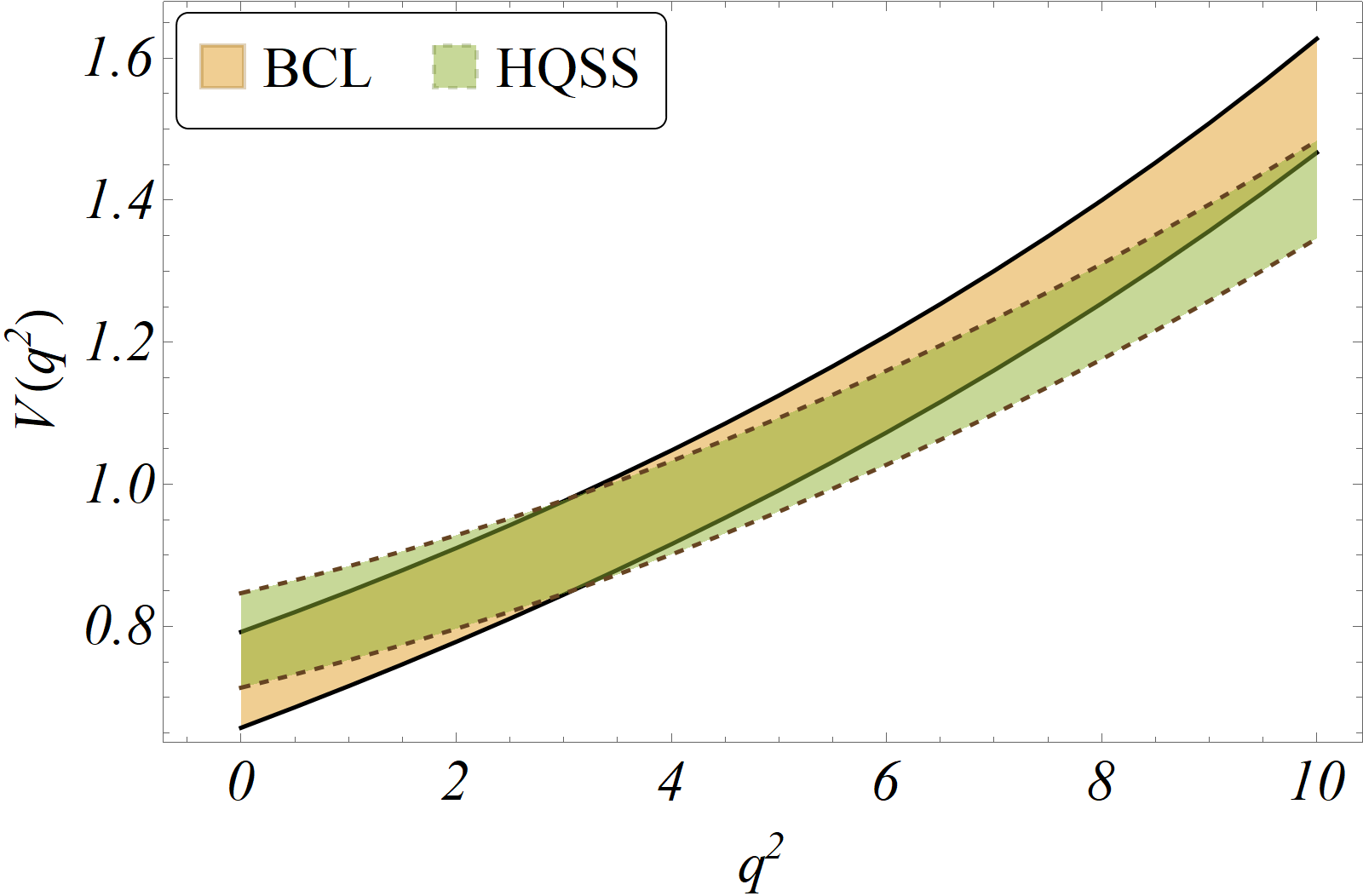
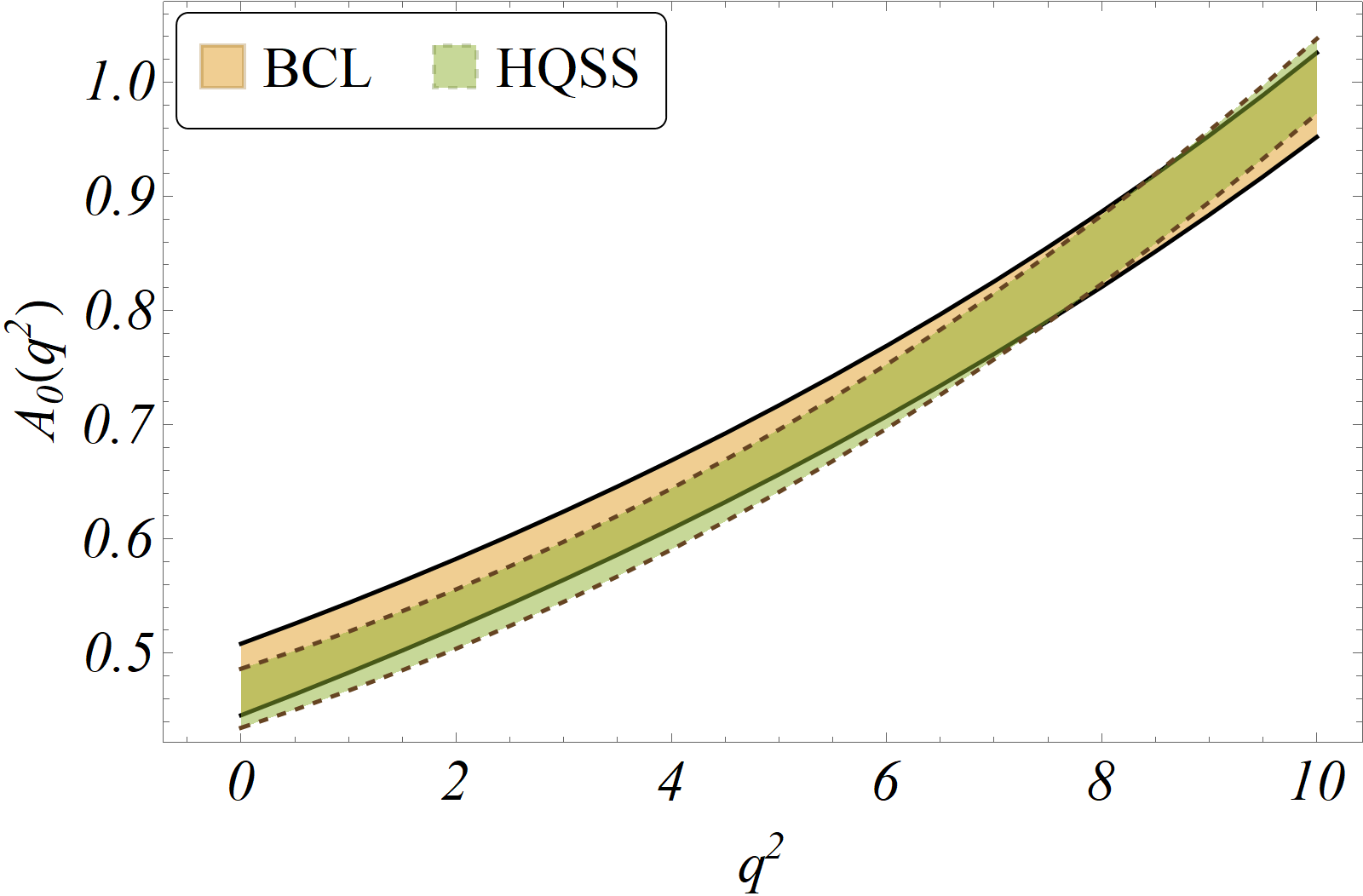
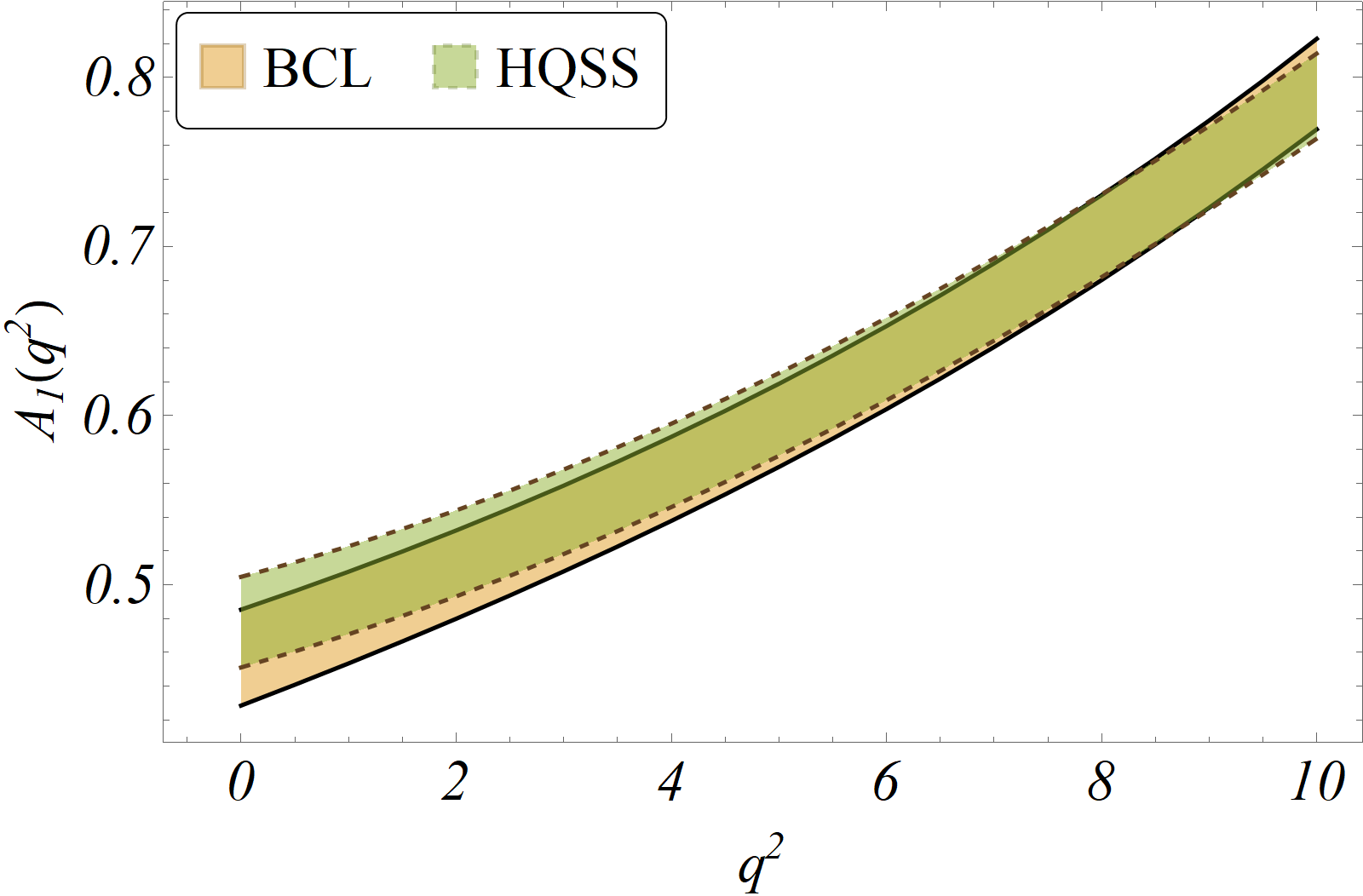
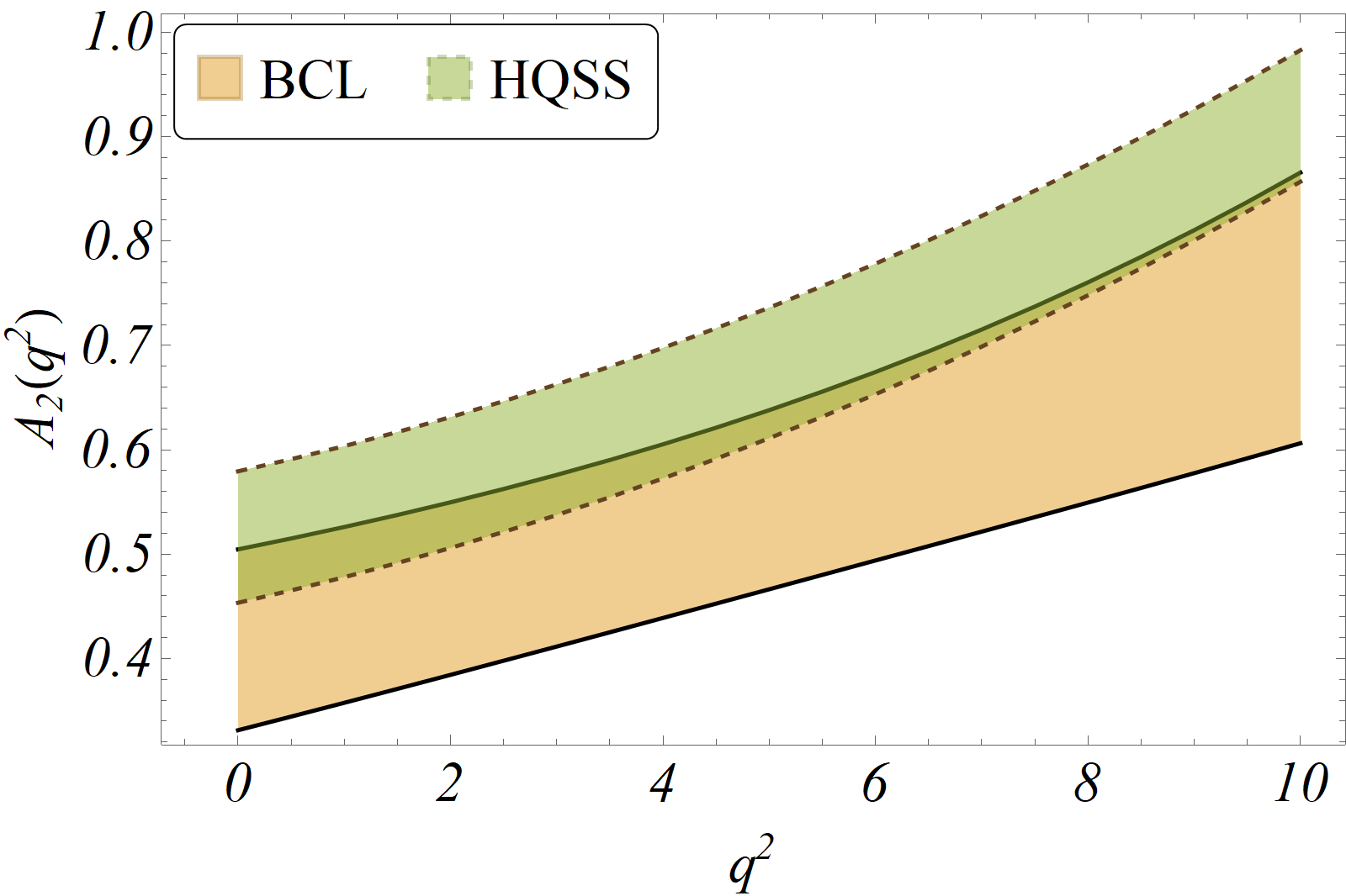
Figure 2: Our $1\sigma$ estimates for the HQSS fit corresponding to the $B_{c}\to J/\psi$ form factors (dashed green bands) compared to the corresponding estimates from Lattice (solid brown bands) in the $m_{b}^{kin.}$ scheme.

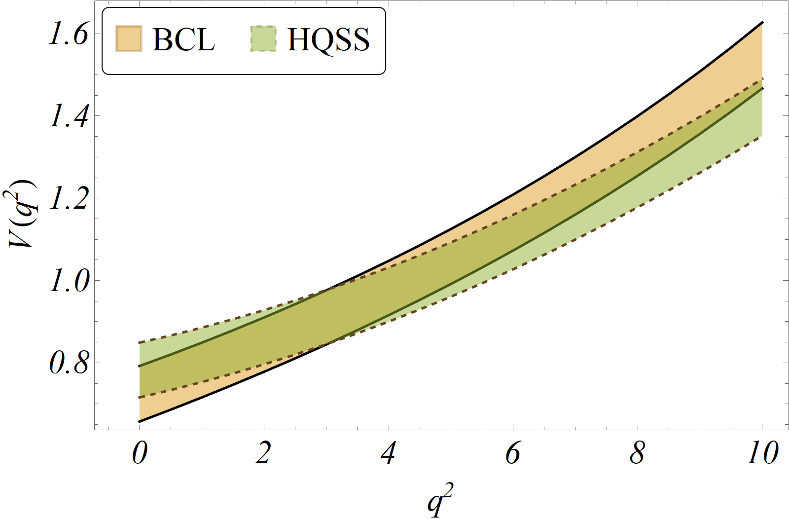
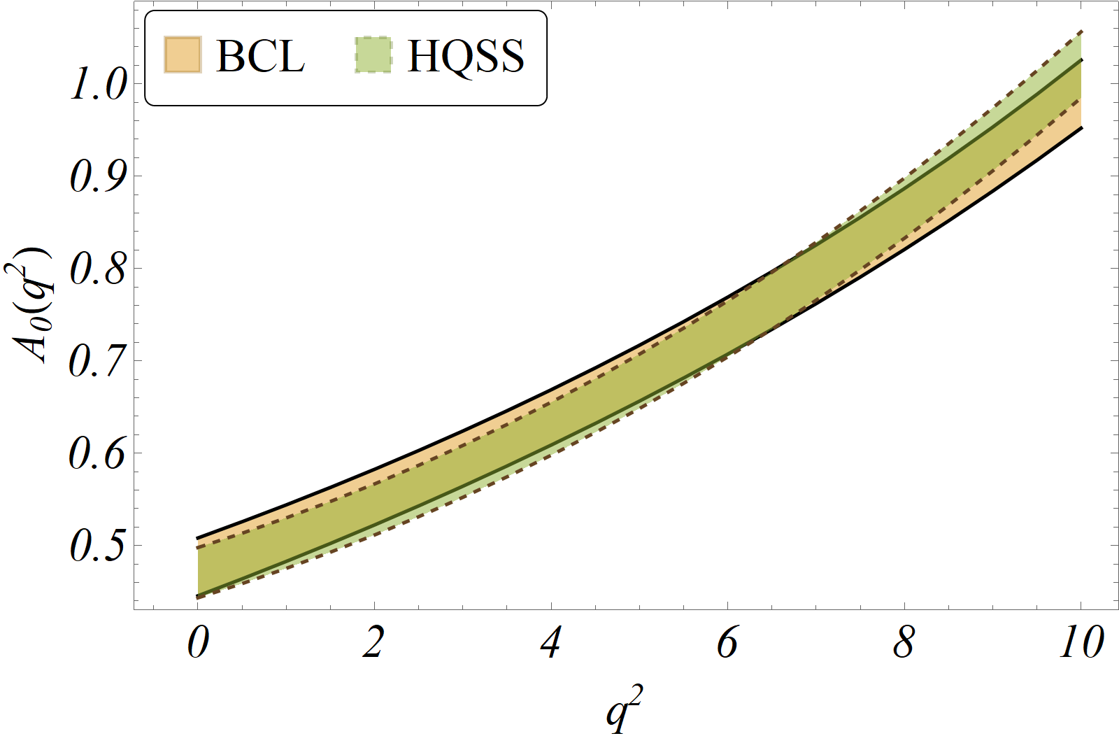
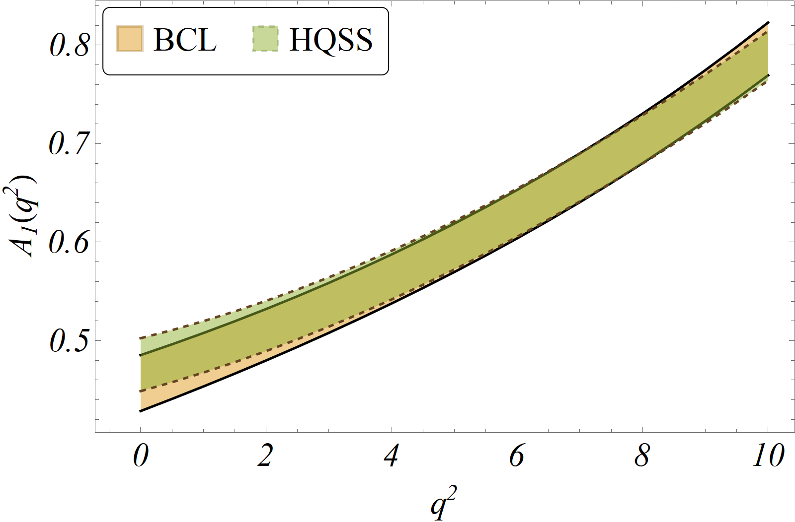
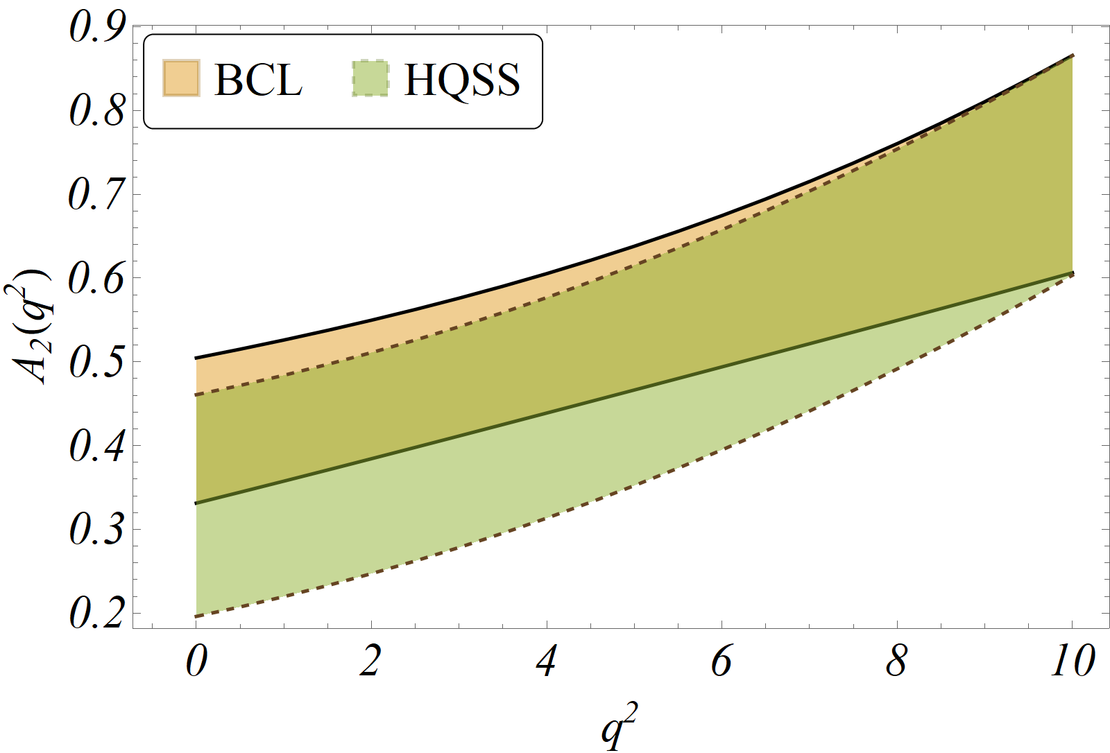
Figure 3: Our $1\sigma$ estimates for the HQSS fit corresponding to the $B_{c}\to J/\psi$ form factors (dashed green bands) compared to the corresponding estimates from Lattice (solid brown bands) in the $m_{b}^{kin.}$ scheme.

Following heavy quark effective theory (HQET), all transition matrix elements between two hadrons with a single heavy-quark (anti-quark) and the same light anti-quark (quark) are related via a universal function called the “Isgur-wise” function. However, this approximation fails for a heavy-heavy bound-state system (as is the case for $B_{c}$ decays). This is due to the fact that both of the constituent quarks are now of comparable masses. This results in a broken Heavy-Quark Flavor Symmetry. However, the decaying and the spectator quarks still retain their separate heavy-quark spin symmetries. And in fact, such systems are described to a better degree of accuracy by non-relativistic dynamics since the valence quarks are heavy. Therefore, the six transition form factors for $B_{c}\to J/\psi$ and $B_{c}\to\eta_{c}$ can be related to a single universal function $\Delta$ via the spin symmetries (instead of the flavour symmetry for the case of the “Isgur-Wise” functions) Jenkins et al. (1993); Kiselev et al. (2000). The trace formalism developed in Falk et al. (1990) is useful to find the relative normalization between these six form factors using NRQCD near the zero recoils Jenkins et al. (1993); Kiselev et al. (2000) and at the non-zero recoils Cohen et al. (2019). Here, the recoil angle $w$ is defined as $w=(m_{B_{c}}^{2}+m_{J/\psi}^{2}-q^{2})/2m_{B_{c}}m_{J/\psi}$. From ref. Cohen et al. (2019), following the leading order NRQCD relations between the form factors in $B_{c}\to J/\psi$ and $B_{c}\to\eta_{c}$, we obtain

$$V = -\frac{m_{B_{c}}+m_{J/\psi}}{2}\frac{c_{V}}{m_{B_{c}}\sqrt{r}}\Delta_{V}(w)\,,$$

$$A_{1} = \frac{m_{B_{c}}}{(m_{B_{c}}+m_{J/\psi})}\sqrt{r}c_{\epsilon}\Delta_{A_{1}}(w)\,,$$

$$A_{2} = -\frac{(m_{B_{c}}+m_{J/\psi})}{2m_{J/\psi}}\sqrt{r}(rc_{1}+c_{2})\Delta_{A_{2}},$$

$$A_{0} = \frac{c_{\epsilon}+(1-wr)c_{1}+(w-r)c_{2}}{2\sqrt{r}}\Delta_{\mathcal{A}_{0}}(w)\,,$$

$$f_{+} = \sqrt{r}\frac{c_{1}^{P}+c_{2}^{P}r^{-1}}{2}\Delta_{+}(w)\,,$$

$$f_{0} = m_{B_{c}}^{2}\sqrt{r}\big{[}(1-wr)c_{1}^{P}+(w-r)c_{2}^{P}\big{]}\Delta_{0}(w)\,.$$ (16)

Here, we have parametrised these $\Delta_{i}(w)$ functions as given below following a Taylor series expansion around $w=1$,

$$\Delta_{i}(w)=\Delta_{i}(1)+(w-1)\Delta(1)^{\prime}+\frac{(w-1)^{2}}{2}\Delta(1)^{\prime\prime}.$$ (17)

The unknown parameters $\Delta_{i}(1)$, $\Delta(1)^{\prime}$ and $\Delta(1)^{\prime\prime}$ can be estimated via a $\chi^{2}$ optimization method using lattice results on $B_{c}\to J/\psi$ form factors. Note that here the parameters $\Delta(1)^{\prime}$ and $\Delta(1)^{\prime\prime}$ are useful in determining the slope of the shapes of the form factors. The definitions for $r$, $k$ and $c_{i}$’s can be obtained from ref. Cohen et al. (2019) and the references therein. According to HQSS near the zero recoil ($w=1$)

$$\Delta_{V}(1)=\Delta_{A_{1}}(1)=\Delta_{A_{2}}(1)=\Delta_{A_{0}}(1)=\Delta_{+}(1)=\Delta_{0}(1)=\Delta.$$ (18)

In order to account for the symmetry-breaking corrections in the limit $w\to 1$, we have kept all the $\Delta_{i}(1)$ different in our fit. However, for simplicity and lack of a sufficient number of inputs, we require $\Delta(1)^{\prime}$ and $\Delta(1)^{\prime\prime}$ to be the same for all the form factors. As we shall see shortly, the $\Delta_{i}$’s are all consistent with each other within their $1\sigma$ confidence intervals (CI).

Pseudo data points for $f^{B_{c}\to\eta_{c}}_{+,0}(q^{2})$
$f_{+}(6)$	$f_{+}(8)$	$f_{+}(10)$	$f_{0}(6)$	$f_{0}(8)$	$f_{0}(10)$
0.767(56)	0.877(56)	1.006(56)	0.667(49)	0.726(46)	0.791(44)

Table 5: Synthetic data for the $B_{c}\rightarrow\eta_{c}$ form factors generated using eq. 17 and the results of $\Delta(1)^{\prime}$ and $\Delta(1)^{\prime\prime}$ given in the third column of tab 4. Also, to generate the numbers, we have used the conservative inputs $\Delta_{+}(w=1)=\Delta_{0}(w=1)=0.844(47)$.

	Fitted Results in Kinetic scheme
BCL coefficients	With NRQCD inputs	Without NRQCD inputs
$a_{0}^{0}$	0.567(27)	0.571(31)
$a_{0}^{1}$	-3.243(598)	-3.173(652)
$a_{+}^{0}$	0.642(31)	0.646(34)
$a_{+}^{1}$	-7.925(557)	-7.876(587)
dof	$3$	$2$
p-Value	$0.621$	$0.427$

Table 6: Fit results for the BCL coefficients $a_{i}^{n}$ corresponding to the $B_{c}\rightarrow\eta_{c}$ transition form factors (we took n=2 for $f_{0}$ and n=1 for $f_{+}$, since higher order coefficients are insensitive to the data) obtained from a fit to the synthetic data generated under HQSS in the kinetic scheme displayed in table 5.

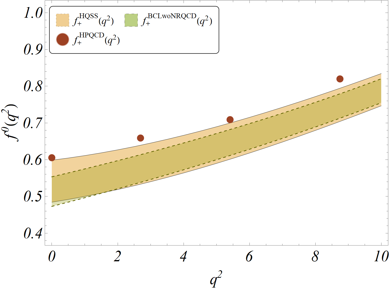
(a)

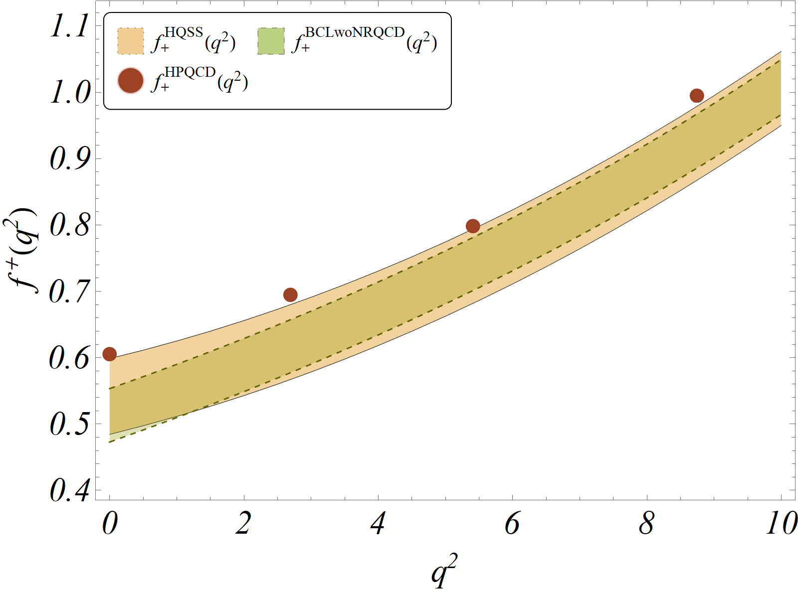
(b)

Figure 4: Our estimates for the $B_{c}\rightarrow\eta_{c}$ form factor plots with a $2\sigma$ error allowed on $\Delta_{\eta_{c}}$ in the $m_{b}^{kin.}$ scheme with HQSS parameters fit result. We overlay the data provided by the HPQCD collaboration Colquhoun et al. (2016). The bands represent the $1\sigma$ region for the corresponding form factors with the brown band representing the form factors corresponding to the HQSS parametrization and the green band specifying the BCL parametrization using the results from the third column of table 6.

We generate synthetic data points for the form factors in $B_{c}\to J/\psi$ decays over the allowed kinematical range using the fit results and the correlations for the same given in ref. Harrison et al. (2020a). Using the generated pseudo data points and their correlations, which are shown in table 18, we carry out the fit using the $\chi^{2}$-minimization procedure to extract the parameters $\Delta_{i}(1)$, $\Delta(1)^{\prime}$ and $\Delta(1)^{\prime\prime}$, respectively. We have generated pseudo data points for all the form factors: $V$, $A_{0}$, $A_{1}$ and $A_{2}$. The $\chi^{2}$ function is defined as :

$$\chi^{2}=\sum_{i,j}(O_{i}^{HQSS}-O_{i}^{lattice})^{T}V_{ij}(O_{j}^{HQSS}-O_{j}^{lattice}).$$ (19)

Where, $(O^{HQSS}-O^{lattice})$ is a column vector whose $i^{th}$ element is the difference between the theoretical expression and the experimental value for the $i^{th}$ observable. $V_{i,j}$ is the covariance matrix, the $i^{th}$ diagonal element of which is the squared-uncertainty corresponding to the lattice estimate for the $i^{t}h$ observable. The $\chi^{2}$ function depends on the concerned parameters through the $O_{i}^{HQSS}$’s.

The corresponding results in the kinetic scheme have been displayed in the second column of table 4. The results obtained in the pole and $\overline{MS}$ schemes are consistent with those obtained in the kinetic scheme. Hence, we have not shown them separately. We note that all the $\Delta_{i}$’s are consistent with each other within their $1\sigma$ CI’s. The corresponding $q^{2}$ shapes of the form factors obtained from the fit results are shown in fig. 2. These shapes have been compared to the respective lattice results. The fit results based on HQSS symmetry can correctly reproduce the slopes for the respective form factors and the corresponding $q^{2}$ distributions for $V(q^{2})$, $A_{0}(q^{2})$, and $A_{1}(q^{2})$. Note that we can correctly reproduce the slope for $A_{2}(q^{2})$ . However, the numerical values at different $q^{2}$ points are marginally consistent with the respective lattice results at 1$\sigma$ CI.

Following the above observation, we have carried out another fit where we have excluded the inputs on $A_{2}(q^{2})$. The corresponding fit result is shown in the third column of table 4. Note that the results are almost identical to the one obtained before in the fit with the pseudo data points on $A_{2}(q^{2})$. Using these results we can obtain the shape of $A_{0}(q^{2})$, $A_{1}(q^{2})$, and $V(q^{2})$, respectively which are shown in figure 3. To obtain the shape of $A_{2}(q^{2})$, we need to fix $\Delta_{A_{2}}(1)$ (see eq.  16), which we obtain directly by solving the eq. $A_{2}(w=1)=0.740(131)$:

$$\Delta_{A_{2}}(1)=0.676\pm 0.120.$$ (20)

Using this result for $\Delta_{A_{2}}(1)$, $\Delta(1)^{\prime}$ and $\Delta(1)^{\prime\prime}$ from table 4 ($3^{rd}$ column), we have obtained the shape of $A_{2}(q^{2})$ which has been shown in the bottom right plot of figure 3. Thus, we are able to reproduce the $q^{2}$ shapes of all four form factors as predicted by lattice from our fits.

Our objective is to obtain the $q^{2}$ shapes of the form factors $f_{+,0}^{B_{c}\to\eta_{c}}(q^{2})$, which in the HQSS framework is parametrized as shown in the relations provided in eqs. 16 and 17, respectively. We need the inputs on $\Delta(1)^{\prime}$, $\Delta(1)^{\prime\prime}$, $\Delta_{+}(1)$ and $\Delta_{0}(1)$ respectively in order to obtain these shapes. The inputs on the parameters $\Delta(1)^{\prime}$ and $\Delta(1)^{\prime\prime}$ can be collected from the fit results provided in table 4. In order to fix the values of $\Delta_{+}(1)=\Delta_{0}(1)$, we use an average over the values of $\Delta_{V}(1)$, $\Delta_{A_{1}}(1)$ and $\Delta_{A_{0}}(1)$ obtained from the fit (the results of which we have shown in the third column of table 4). Following this method we obtain

$$\Delta_{+}(w=1)=\Delta_{0}(w=1)=0.844(47).$$ (21)

To keep our estimates conservative, we double the error displayed in eq. 21. The corresponding shapes of $f_{+}(q^{2})$ and $f_{0}(q^{2})$ are shown in figs. 4a and 4b respectively. The shapes obtained are extremely consistent with the preliminary lattice data points (without error) provided in ref. Colquhoun et al. (2016).

As we know, the $q^{2}$ shapes of $f_{+,0}(q^{2})$ can also be obtained using the BCL parametrization Bourrely et al. (2009) for the respective form factors. In this parametrization, both the form factors are written as a polynomial series in powers of $q^{2}$.

$$f_{i}(q^{2})=\frac{1}{P(q^{2})}\sum_{k=0}^{n}a_{i}^{k}z^{k}(q^{2},t_{0})$$ (22)

with $i=0,+$ and

$$z(q^{2},t_{0}) = \frac{\sqrt{t_{+}-q^{2}}-\sqrt{t_{+}-t_{0}}}{\sqrt{t_{+}-q^{2}}+\sqrt{t_{+}-t_{0}}},$$

$$t_{0} = t_{+}\left(1-\sqrt{1-\frac{t_{-}}{t_{+}}}\right).$$ (23)

In the above, $t_{\pm}=(m_{B_{c}}\pm{\eta_{c}})^{2}$ and $P(q^{2})=1-q^{2}/m_{R}^{2}$. $m_{R}$ represents the masses of the low-lying $B_{c}$ resonances. We use $m_{R}=6.34$ GeV and $6.71$ GeV for $f_{+}$ and $f_{0}$ respectively in accordance with ref. Leljak et al. (2019). The goal here is the extraction of the BCL expansion coefficients $a_{i}$’s. To that end, we first generate pseudo data points for $f_{+,0}(w)$ following eqs. 16 and 17 respectively using the fit results of $\Delta(1)^{\prime}$ and $\Delta(1)^{\prime\prime}$ given in table 4 and $\Delta_{+}(1)$, $\Delta_{0}(1)$ from eq. 21. These data points are provided in table 5, and can be compared to more precise lattice estimates in the future. We have checked that we get identical results using the results in the second column of table 4, which we have not shown. We then fit the BCL coefficients using these pseudo datapoints, the results of which we have presented in table 6. We reduce the number of free parameters from six to five by using the QCD relation $f_{+}(0)=f_{0}(0)$. The respective $q^{2}$ shapes obtained using these fit results and the related correlations are shown in figs. 4a and 4b respectively. As expected, these agree with the one obtained using HQSS expansion and the preliminary data from lattice. We obtain the following values at $q^{2}=0$:

$$f_{+}^{B_{c}\to\eta_{c}}(q^{2}=0)=f_{0}^{B_{c}\to\eta_{c}}(q^{2}=0)=\begin{cases}0.513\pm 0.040\ \ \ \text{(BCL)},\\ 0.541\pm 0.058\ \ \ \text{(HQSS)}.\end{cases}$$ (24)

Also, using this result for the form factors, we have predicted the lepton flavour universality conserving observable $R(\eta_{c})=\frac{\Gamma(B_{c}^{-}\rightarrow\eta_{c}\tau\bar{\nu}_{\tau})}{\Gamma(B_{c}^{-}\rightarrow\eta_{c}\mu^{-}\bar{\nu}_{\mu})}$ which is given by

$$R(\eta_{c})=0.302\pm 0.010.$$ (25)

The estimated error is only 3%, which is the most precise theory estimate so far, even after we have doubled the error on the HQSS parameters. Our prediction can be compared to the earlier predictions:

$$R(\eta_{c})=\begin{cases}0.31^{+0.04}_{-0.02}\ \ \ \ \text{\cite[cite]{\@@bibref{Authors Phrase1YearPhrase2}{Murphy:2018sqg}{\@@citephrase{(}}{\@@citephrase{)}}}},\\ 0.30\pm 0.05\ \ \text{\cite[cite]{\@@bibref{Authors Phrase1YearPhrase2}{Cohen:2019zev}{\@@citephrase{(}}{\@@citephrase{)}}}},\\ 0.29\pm 0.05\ \ \text{ \cite[cite]{\@@bibref{Authors Phrase1YearPhrase2}{Berns:2018vpl}{\@@citephrase{(}}{\@@citephrase{)}}}}.\end{cases}$$ (26)

Note that our prediction agrees with all these predictions. We also obtain $R_{\eta_{c}}$ following other schemes like the $\overline{MS}$ and pole-mass schemes. The corresponding result is extremely consistent with the one obtained from the kinetic scheme provided in eq. 25.

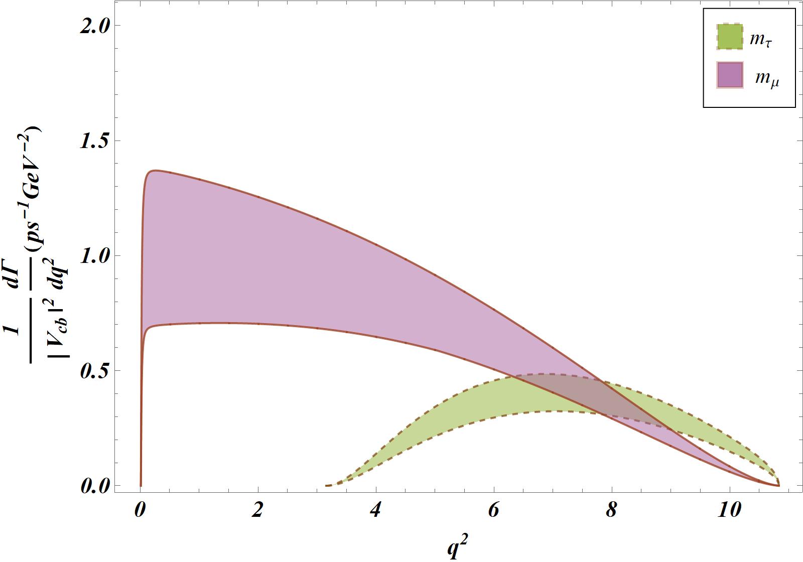
Figure 5: 1$\sigma$ bands for the differential decay distributions corresponding to semileptonic $B_{c}\to\eta_{c}$ decays with a tauon (green) or a muon (purple) in the final state.

Using the estimates on the shape of $f_{+,0}(q^{2})$ we have predicted the shape of $\frac{1}{|V_{cb}|^{2}}\frac{d\Gamma(B_{c}^{-}\to\eta_{c}\ell^{-}\bar{\nu})}{dq^{2}}$ with $\ell=\tau,\mu(e)$. The corresponding shapes are displayed in fig. 5. The overall normalization is dependent on the value of $|V_{cb}|^{2}$. Our estimates for the uncertainties are rather large at present. We expect this to improve with more precise inputs on the form factors so that the shape can be compared to future experiments. We also provide the $q^{2}$ integrated branching fraction $\mathcal{B}(B_{c}^{-}\to\eta_{c}\ell^{-}\bar{\nu})$:

$$\frac{1}{|V_{cb}|^{2}}\mathcal{B}(B_{c}^{-}\to\eta_{c}\tau\bar{\nu})=(1.040\pm 0.100),\ \ \ \ \frac{1}{|V_{cb}|^{2}}\mathcal{B}(B_{c}^{-}\to\eta_{c}\mu^{-}\bar{\nu})=(3.447\pm 0.421).~{}~{}~{}$$ (27)

With $|V_{cb}|=0.0403(5)$ Ray and Nandi (2023) we obtain for the SM

$$\mathcal{B}(B_{c}^{-}\to\eta_{c}\tau^{-}\bar{\nu})=(1.689\pm 0.168)\times 10^{-3},\ \ \ \ \mathcal{B}(B_{c}^{-}\to\eta_{c}\mu^{-}\bar{\nu})=(5.598\pm 0.698)\times 10^{-3}.~{}~{}~{}~{}$$ (28)

All these predictions can be tested in future experiments, which will be helpful in understanding the predictive power of HQSS.

III.2 Extractions of $\psi^{R}_{M}(0)$ with $M=B_{c},J/\psi,\eta_{c}$

In this subsection, we will discuss the method to extract the radial wave functions $\psi^{R}_{B_{c}}(0)$, $\psi^{R}_{J/\psi}(0)$ and $\psi^{R}_{\eta_{c}}(0)$ at very small interquark distances using lattice inputs for the form factors and the experimental data mentioned in subsection II.2. We have done the analyses considering the experimental data specified in table 3 and the synthetic data points (generated at $q^{2}=0$) given in table 2 obtained from the lattice results. In order to estimate these parameters, we construct a likelihood function comprising of the the radial wave functions as parameters. These parameters enter the likelihood function via the expressions for the three observables BR($J/\psi\to\gamma\gamma\gamma$), BR($J/\psi\to e^{+}e^{-}$), BR($\eta_{c}\to\gamma\gamma$) and the expressions for the $B_{c}\to J/\psi(\eta_{c})$ form factors at $q^{2}$=0. In this analysis, we construct a $\chi^{2}$ function defined as

$$\chi^{2}=\sum_{i}\frac{(O_{i}^{NRQCD}-O_{i}^{expt})^{2}}{\sigma_{i}^{2}}+\sum_{i,j}(O_{i}^{NRQCD}-O_{i}^{lattice})^{T}V_{ij}(O_{j}^{NRQCD}-O_{j}^{lattice}).$$ (29)

Here $O_{i}^{NRQCD}$s represent the theory expressions for the form factors and the decay rates calculated in the NRQCD effective theory. $O_{i}^{expt}$ and $O_{i}^{lattice}$ represent the relevant experimental data and the lattice inputs respectively. The $\sigma_{i}$ in the denominator of the first term represents the error in the experimental measurements at 1$\sigma$. Note that here we use experimental data which are not correlated. We have also carried out two types of fits depending on whether or not the inputs on $f_{+,0}^{B_{c}\to\eta_{c}}(q^{2}=0)$ obtained in subsection III.1 are used in the analyses. The extracted values of the radial wave functions from both fits are consistent with each other.

The fit results obtained after minimizing the $\chi^{2}$ function defined in eq. 29 are shown in table 7 for the kinetic, $\overline{MS}$ and pole-mass schemes respectively. To obtain these results, we have not included the inputs on $f_{+,0}^{B_{c}\to\eta_{c}}(q^{2}=0)$. This is because the form factors calculated in NRQCD are highly sensitive to masses of the $b$ and $c$ quarks. As discussed earlier, the perturbative corrections at order $\alpha_{s}$ and the first-order relativistic corrections to the form factors calculated in NRQCD are available. To check the impact of these corrections on the extracted values of $\psi^{R}_{M}(0)$, we present our results considering the NRQCD form factors at LO, LO+NLO, and LO+NLO+RC separately. Furthermore, we consider a $\pm$20% additional error due to the missing (QCD and relativistic) higher order corrections to the form factors calculated in NRQCD in an additional fit. It is to be noted that the fit quality in the kinetic scheme is relatively better than that in the pole mass and $\overline{MS}$ schemes.

The $B_{c}\to J/\psi$ form factors are sensitive to the product: $\psi^{R}_{B_{c}}(0)\psi^{R}_{J/\psi}(0)$. It is thus possible to get constraints on $\psi^{R}_{J/\psi}(0)$ and $\psi^{R}_{\eta_{c}}(0)$ directly from the experimental data given in Table 3. Hence, a combination of these experimental data and the lattice input on the form factors (at $q^{2}=0$) will be useful to constrain $\psi^{R}_{B_{c}}(0)$, $\psi^{R}_{J/\psi}(0)$ and $\psi^{R}_{\eta_{c}}(0)$ simultaneously. However, $\psi^{R}_{B_{c}}(0)$ will be constrained mainly by lattice. This is evident from our results: the extracted values of $\psi^{R}_{B_{c}}(0)$ gradually reduce while $\psi^{R}_{J/\psi}(0)$ remain fixed with the inclusion of higher order corrections to $B_{c}\to J/\psi$ form factors. The reduction in the values of $\psi^{R}_{B_{c}}(0)$ is because the higher order corrections in all these form factors appear with a plus sign. There are hence no relative numerical cancellations between different orders. Each of the parameters $\psi_{B_{c}}^{R}(0)$ and $\psi_{\eta_{c}}^{R}(0)$ can be extracted with an error of about $5$%. However we obtain a very precise value for $\psi_{J/\psi}^{R}(0)$ with an error of about $1$%. The extracted values of the form factors in the different fits provided in Table 7 are presented in table 8. Note that in the fits without the additional corrections, apart from $A_{2}(0)$, the other three form factors are consistent with the respective lattice inputs at the 1-$\sigma$ CI. Not surprisingly though, the additional corrections render the form factors consistent with the respective lattice inputs at their 1-$\sigma$ CI.

	Schemes	$\psi^{R}_{B_{c}}$(0)	$\psi^{R}_{J/\psi}(0)$	$\psi^{R}_{\eta_{c}}(0)$	$\delta_{V}$	$\delta_{A0}$	$\delta_{A2}$	p-value
(I) LO	$\overline{\textbf{MS}}$	0.404(24)	1.002(5)	0.848(32)	$-$	$-$	$-$	$0.037$
	Pole	0.437(26)	1.239(10)	1.067(41)	$-$	$-$	$-$	$0.002$
	Kinetic	0.680(41)	0.909(7)	0.760(29)	$-$	$-$	$-$	$\bf 0.156$
(II) LO+NLO	$\overline{\textbf{MS}}$	0.304(18)	1.002(5)	0.848(32)	$-$	$-$	$-$	$0.032$
	Pole	0.341(21)	1.239(10)	1.067(41)	$-$	$-$	$-$	$0.002$
	kinetic	0.496(30)	0.909(7)	0.760(29)	$-$	$-$	$-$	$\bf 0.160$
(III) LO+NLO+RC	$\overline{\textbf{MS}}$	0.232(14)	1.002(5)	0.848(32)	$-$	$-$	$-$	$0.025$
	Pole	0.239(15)	1.239(10)	1.067(41)	$-$	$-$	$-$	$0.001$
	kinetic	0.417(25)	0.909(7)	0.760(29)	$-$	$-$	$-$	$\bf 0.141$
Fit-III	$\overline{\textbf{MS}}$	0.227(21)	1.002(5)	0.848(32)	0.029(155)	0.089(146)	-0.126(174)	$0.043$
	Pole	0.233(21)	1.239(10)	1.067(41)	0.006(156)	0.103(149)	-0.115(176)	$0.002$
$\pm$ add. err.	Kinetic	0.408(39)	0.909(7)	0.760(29)	0.064(154)	0.066(143)	-0.141(172)	$\bf 0.240$

Table 7: Fit results for radial wave functions corresponding to the $B_{c}$, $J/\psi$ and $\eta_{c}$ mesons.

Predictions using the fit results
Form Factors	Kinetic Scheme		Pole Scheme		$\overline{\textbf{MS}}$ Scheme		Lattice data
	LO + NLO	With add.	LO+NLO	With add.	LO+NLO	With add.
	+ RC	err.	+RC	err.	+RC	err.
$V^{J/\psi}\text{(0)}$	$0.693(42)$	$0.704(61)$	$0.734(44)$	$0.718(60)$	$0.719(43)$	$0.712(60)$	$0.725(68)$
$A_{0}^{J/\psi}\text{(0)}$	$0.460(28)$	$0.469(31)$	$0.453(27)$	$0.467(31)$	$0.456(27)$	$0.468(31)$	$0.477(32)$
$A_{1}^{J/\psi}\text{(0)}$	$0.512(31)$	$0.480(72)$	$0.489(29)$	$0.477(68)$	$0.498(30)$	$0.478(69)$	$0.457(29)$
$A_{2}^{J/\psi}\text{(0)}$	$0.557(33)$	$0.501(59)$	$0.541(32)$	$0.495(56)$	$0.549(33)$	$0.498(57)$	$0.417(88)$
$f_{+}^{\eta_{c}}\text{(0)=}f_{0}^{\eta_{c}}\text{(0)}$	$0.490(35)$	$-$	$0.429(30)$	$-$	$0.452(32)$	$-$	$-$

Table 8: The predictions of the respective form-factors (in NRQCD) at maximum recoil obtained using the fit results in different schemes.

One can note from table 7 that the extracted values of $J/\psi$ and $\eta_{c}$ wave functions do not change in the fit with additional $20$% error to the NRQCD form factors, whereas the best-fit point of $\psi^{R}_{B_{c}}(0)$ is lowered by $\approx$ 2% and the error increased by $\approx$ 4%. Therefore, even after considering an error around 20% for the missing higher order corrections, $\psi^{R}_{B_{c}}(0)$ can be extracted with an error of 10%. As a conservative estimate, we will consider an error of approximately 15% in the extracted value of $\psi^{R}_{B_{c}}(0)$ in Fit-III in the next part of our analyses. This was about 6% in the actual fit. This means we are adding an error of nearly about 10% on account of the missing higher-order pieces. For example in the kinetic scheme, we consider $\psi_{B_{c}}(0)=0.417\pm 0.063$ as a conservative estimate.

Inputs	$R^{J/\psi}_{\eta_{c}}=\psi^{R}_{J/\psi}(0)/\psi^{R}_{\eta_{c}}(0)$
	Kin. Scheme	$\overline{\bf MS}$ Scheme	Pole scheme
$\text{Form factors (LO+NLO+RC)}:$ Lattice	0.863(70)	0.802(65)	0.763(61)
$\text{Form factors (LO+NLO)}:$ Lattice	0.891(72)	0.936(76)	1.010(80)
Expt. data (tab. 3 )	1.196(45)	1.172(44)	1.126(42)

Table 9: The extracted values of $R^{J/\psi}_{\eta_{c}}=\frac{\psi^{R}_{J/\psi}(0)}{\psi^{R}_{\eta_{c}}(0)}$ using lattice and experimental data separately.

We have repeated Fit-III in table 7 including the inputs on $f_{+,0}^{B_{c}\to\eta_{c}}(q^{2}=0)$ given in eq. 24. The result in the kinetic scheme is given by

$$\psi_{B_{c}}^{R}(0)=0.419\pm 0.016,\ \ \ \psi_{J/\psi}^{R}(0)=0.9088\pm 0.0071,\ \ \ \psi_{\eta_{c}}^{R}(0)=0.765\pm 0.027.$$ (30)

Note that these fitted values are consistent with the corresponding ones in table 7. However, the inclusion of these inputs reduces the error in the estimates of the radial wave functions. We have similar conclusions for the results obtained in both the other schemes. Hence, we will not present them separately.

Note that in the ratios of the NRQCD form factors $F_{i}^{B_{c}\to J/\psi}/F_{i}^{B_{c}\to\eta_{c}}$, the radial wave function of the $B_{c}$ meson will cancel and it will become sensitive to $R^{J/\psi}_{\eta_{c}}=\psi^{R}_{J/\psi}(0)/\psi^{R}_{\eta_{c}}(0)$. In this work, we have created pseudo data points for these form factor ratios (at $q^{2}=0$) using the information from lattice and HQSS (subsection III.1). Using these pseudo data points, we have extracted $R^{J/\psi}_{\eta_{c}}$ which are presented in the first two rows of table 9. We have presented the results in three different mass schemes and for the NRQCD form factors defined with “LO+NLO” and “LO + NLO +RC” contributions respectively. We have also quoted the respective errors at their 1$\sigma$ CI. The results show that the best-fit values of $R^{J/\psi}_{\eta_{c}}$ is slightly less than 1. The values are also consistent in different mass schemes even after considering the relativistic corrections to the form factors. We have extracted the same ratio using only the experimental data shown in table 3. The results are shown in the third row of table 9. Note that the extracted values of $R^{J/\psi}_{\eta_{c}}$ are above those obtained using the inputs on the form factors, and they are inconsistent with each other within their 1$\sigma$ CI.

III.3 Decay constants and $\mathcal{B}(B_{c}^{-}\to\ell^{-}\bar{\nu})$

In the NRQCD approach, the detailed theoretical expressions for the decay constants $f_{B_{c}}$, $f_{J/\psi}$ and $f_{\eta_{c}}$ are given as follows Wang and Zhu (2015):

$$f_{J/\psi}=\sqrt{\frac{3}{2m_{c}\pi}}\psi^{R}_{J/\psi}(0)\left[\left(1-\frac{8}{3}\,\frac{\alpha_{s}}{\pi}\right)^{2}\left(1-\frac{1}{6}\,\langle v^{2}\rangle_{J/\psi}\right)^{2}\times\frac{1}{(1+\langle v^{2}\rangle_{J/\psi})}\right]^{1/2},$$ (31)

$$f_{\eta_{c}}=\sqrt{\frac{3}{2m_{c}\pi}}\psi^{R}_{\eta_{c}}(0)\left[1+\frac{\alpha_{s}}{\pi}\frac{\pi^{2}-20}{3}+\langle v^{2}\rangle_{\eta_{c}}\left(-\frac{4}{3}+\frac{\alpha_{s}}{\pi}\frac{1}{27}(48\ln\frac{\mu_{\Lambda}^{2}}{m_{Q}^{2}}-96\ln 2-15\pi^{2}+196)\right)\right]^{1/2},$$ (32)

$$f_{B_{c}}=\sqrt{\frac{2}{m_{B_{c}}}}\Bigg{[}c_{0}^{f}\langle 0|\chi_{c}^{\dagger}\psi_{b}|\overline{B_{c}}(P)\rangle+\frac{c_{2}^{f}}{m_{B_{c}}^{2}}\langle 0|\chi_{c}^{\dagger}\bigg{(}-\frac{i}{2}\mathcal{D}\bigg{)}^{2}\psi_{b}|\overline{B_{c}}(P)\rangle+\mathcal{O}(v^{4})\Bigg{]}.$$ (33)

In eq. 33, the coefficients $c_{0}^{f}$, $c_{2}^{f}$ are taken from ref Wang and Zhu (2015) and the matrix elements are defined in eqs. 5 and II.1 respectively. Therefore, the decay constants are also sensitive to the mesonic wave function $\psi^{R}_{M}(0)$. In principle, one could use these inputs to constrain the wave functions. The corresponding lattice inputs are available which are shown in the second column in table 10. Alternatively, one could predict these decay constants after extracting the wave functions using some other inputs. We have tried both and discuss the outcome in what follows.

Decay Const. (MeV)	Lattice estimate	QCDSR	Our prediction:
			Kin. Scheme
$f_{B_{c}}$	434 (15) McNeile et al. (2012); Colquhoun et al. (2015)	-	$\begin{array}[]{l}0.147(29)\\ 0.174(11)\end{array}$
$f_{J/\psi}$	405(6) Donald et al. (2012)	401(36) Bečirević et al. (2014)	349(50)
$f_{\eta_{c}}$	394.7(2.4) Davies et al. (2010)	309(39) Bečirević et al. (2014)	292(43)

Table 10: Lattice results for the decay constants used in our analysis.

We have predicted the decay constants in the above equations using the results from table 7. We have extracted $\psi^{R}_{B_{c}}(0)$ from the NRQCD form factors defined with and without the relativistic corrections, which are presented as Fit-III and Fit-II respectively, in table 7. Using both these results, we have estimated $f_{B_{c}}$, which are presented in table 10. We have also presented estimates for $f_{J/\psi}$ and $f_{\eta_{c}}$. In the same table, we have shown the corresponding lattice predictions. Note that the lattice estimates are higher than the values we have obtained in our analysis. In particular, the central values of $f_{B_{c}}$ differ by more than 50%. However, the QCDSR predictions for $f_{J/\psi}$ and $f_{\eta_{c}}$ given in the same table are consistent with our obtained values. In addition, we have estimated the ratio $R^{J/\psi}_{\eta_{c}}$ defined in table 9 using the lattice inputs on $f_{J/\psi}$ and $f_{\eta_{c}}$. The obtained values are given by

$$R^{J/\psi}_{\eta_{c}}=\begin{cases}1.026\pm 0.016\ \ \text{(Kinetic scheme)},\\ 1.005\pm 0.016\ \ \text{($\overline{MS}$ scheme)},\\ 0.966\pm 0.016\ \ \ \text{(Pole mass scheme)}.\end{cases}$$ (34)

These numbers are relatively more precise than those obtained in table 9 and the values lie in between those we get using the lattice form factor and experimental data respectively.

Decay Mode	Predictions using	Predictions using	Predictions in Wang and Zhu (2015)
	$f_{B_{c}}=0.147(29)$ (table 10)	$f_{B_{c}}=0.174(11)$ (table 10)
$10^{2}\times\mathcal{B}(B_{c}\to\tau\nu)$	$0.248(99)$	$0.350(42)$	$1.80^{+0.03}_{-0.04}$
$10^{5}\times\mathcal{B}(B_{c}\to\mu\nu)$	$1.035(414)$	$1.461(177)$	$7.53^{+0.14}_{-0.16}$

Table 11: Predictions for the leptonic decays of the $B_{c}$ meson.

Using our estimates for $f_{B_{c}}$, we present our predictions for the branching fraction of $B_{c}\to\ell\nu$ decays with $(\ell=\tau,\mu)$. The corresponding expression for the decay rate is given by

$$\Gamma(B_{c}\rightarrow\ell\nu)=\frac{G_{F}^{2}}{8\pi^{2}}|V_{cb}|^{2}f_{B_{c}}^{2}m_{B_{c}}^{3}\frac{m_{\ell}^{2}}{m_{B_{c}}^{2}}\bigg{(}1-\frac{m_{\ell}^{2}}{m_{B_{c}}^{2}}\bigg{)}^{2}$$ (35)

The decays of pseudoscalar mesons into light lepton pairs are helicity suppressed, i.e. their decay widths are suppressed by $\frac{m_{\ell}^{2}}{m_{B_{c}}^{2}}$. The results are shown in table 11. As expected our predicted values are much lower than what one can obtain using the lattice result for $f_{B_{c}}$. They are also lower than those obtained in Wang and Zhu (2015) where $f_{B_{c}}$ has been defined in NRQCD. However, they have used $\psi^{R}_{B_{c}}(0)\approx 1.28$ which is almost three times larger than what we have obtained using the lattice inputs.

Following the observation made above, we can comment that the simultaneous explanation of the lattice data for the $B_{c}\to J/\psi$ form factors and the decay constants is not possible currently. We have carried out a fit using all these inputs on form factors and decay constants. The results had very low $p$-values as per our expectations. Assuming no error on behalf of the lattice collaborations, the reason for such a mismatch could be the unknown higher-order pieces in the form factors predicted by NRQCD. It is important to note that for the NRQCD form factors the corrections at order $\alpha_{s}$ are being cross-checked. However, the relativistic corrections have not been subjected to any such check thus far. This is something that should be done but is outside the scope of this work. For a similar reason, one may need to cross check the higher order pieces in the NRQCD expression for the decay constant obtained in ref. Wang and Zhu (2015).

In this paper, we have done a toy analysis where we have parametrised the relativistic corrections in the $B_{c}\to J/\psi$ form factors as

$$F_{i}(q^{2})=F_{i}^{LO}(q^{2})\bigg{[}1+\frac{\alpha_{s}}{4\pi}f_{i,\alpha_{s}}(s,\gamma)+\frac{m_{c}^{2}|v|^{2}}{4m_{b}^{2}}\delta_{1i}+\frac{m_{c}^{2}|v^{\prime}|^{2}}{(m_{b}+m_{c})^{2}}\delta_{2i}\bigg{]},$$ (36)

where $\delta_{i}$’s are the free parameters which will be obtained from the fit to lattice inputs and experimental data discussed earlier. We have also added unknown parameters in the NRQCD expressions for the decay constants to take care of the missing higher-order pieces. We fit these parameters alongside $\delta_{i}$’s defined in eq. 36 from the available inputs. We incorporate lattice inputs for $B_{c}\to J/\psi$ form factors at $q^{2}=0$, $BR(J/\psi\to e^{+}e^{-})$, $BR(J/\psi\to\gamma\gamma\gamma)$, $BR(\eta_{c}\to\gamma\gamma)$, and the lattice inputs on the decay constants $f_{B_{c}}$. The fit results are shown in table 12. To explain the available inputs on the form factors, we need large relativistic corrections in all the form factors ($\approx 70$%) along with a relative sign difference with the respective (LO + NLO) results. However, to explain the available inputs in the decay constants, the unknown higher-order pieces are relatively small as compared to those in the form factors. The available relativistic corrections in ref. Zhu et al. (2017) are large but appear with the same sign as that of the respective (LO+NLO) results. In addition, we now obtain relatively large values for $\psi_{B_{c}}^{R}(0)$, which is consistent with the QCD model predictions mentioned earlier. We will conclude this section by stating that a further detailed understanding of all the inputs is required to understand these discrepancies.

Fit results and the respective predictions in NRQCD in the different scheme.
Fit results				Predictions using the fit results
Parameters	Kinetic	Pole mass	$\overline{\bf MS}$	Form-factors	kinetic mass	Pole mass	$\overline{\bf MS}$
	Scheme	Scheme	Scheme	$\&$	Scheme	Scheme	Scheme
				decay constants
$\psi_{B_{c}}^{R}\text{(0)}$	$1.232(143)$	$1.305(160)$	$1.268(151)$	$V^{J/\psi}\text{(0)}$	$0.726(68)$	$0.725(68)$	$0.725(68)$
$\psi_{J/\psi}^{R}\text{(0)}$	$0.906(125)$	$1.406(202)$	$1.068(153)$	$A_{0}^{J/\psi}\text{(0)}$	$0.478(32)$	$0.477(32)$	$0.477(32)$
$\psi_{\eta_{c}}^{R}\text{(0)}$	$0.758(116)$	$1.232(211)$	$0.900(143)$	$A_{1}^{J/\psi}\text{(0)}$	$0.457(29)$	$0.457(29)$	$0.457(29)$
$10^{-2}\times\delta_{1V}$	$-0.114(979)$	$-0.094(971)$	$-0.111(975)$	$A_{2}^{J/\psi}\text{(0)}$	$0.421(87)$	$0.418(88)$	$0.418(88)$
$10^{-2}\times\delta_{1A_{0}}$	$-0.114(979)$	$-0.090(971)$	$-0.106(975)$	$f_{B_{c}}$	$0.434(15)$	$0.434(15)$	$0.434(15)$
$10^{-2}\times\delta_{1A_{1}}$	$-0.129(979)$	$-0.097(971)$	$-0.115(975)$	$f_{J/\psi}$	$0.349(48)$	$0.437(63)$	$0.381(54)$
$10^{-2}\times\delta_{1A_{2}}$	$-0.139(979)$	$-0.101(971)$	$-0.119(975)$	$f_{\eta_{c}}$	$0.292(44)$	$0.361(62)$	$0.315(50)$
$10^{-2}\times\delta_{2V}$	$-1.098(441)$	$-0.768(480)$	$-0.963(452)$
$10^{-2}\times\delta_{2A_{0}}$	$-1.099(433)$	$-0.733(480)$	$-0.927(451)$
$10^{-2}\times\delta_{2A_{1}}$	$-1.243(428)$	$-0.787(479)$	$-0.999(451)$
$10^{-2}\times\delta_{2A_{2}}$	$-1.336(440)$	$-0.819(480)$	$-1.039(452)$
$\delta_{J\psi ee}$	$-0.0006(932)$	$-0.009(94)$	$-0.007(94)$
$\delta_{J\psi\gamma\gamma\gamma}$	$0.035(39)$	$0.032(39)$	$0.032(39)$
$\delta_{f_{Bc}}$	$0.010(100)$	$0.002(100)$	$0.003(100)$
dof	$5$	$5$	$5$
p-Value	$\bf 0.896$	$\bf 0.980$	$\bf 0.951$

Table 12: Fit results for the radial wave functions corresponding to the $B_{c}$, $J/\psi$ and $\eta_{c}$ mesons and the predictions of the respective form-factors (in NRQCD) at maximum recoil obtained using the fit results in different schemes.

III.4 Test of NP in $B_{c}^{-}\to J/\psi(\eta_{c})\tau^{-}\bar{\nu}_{\tau}$ decays

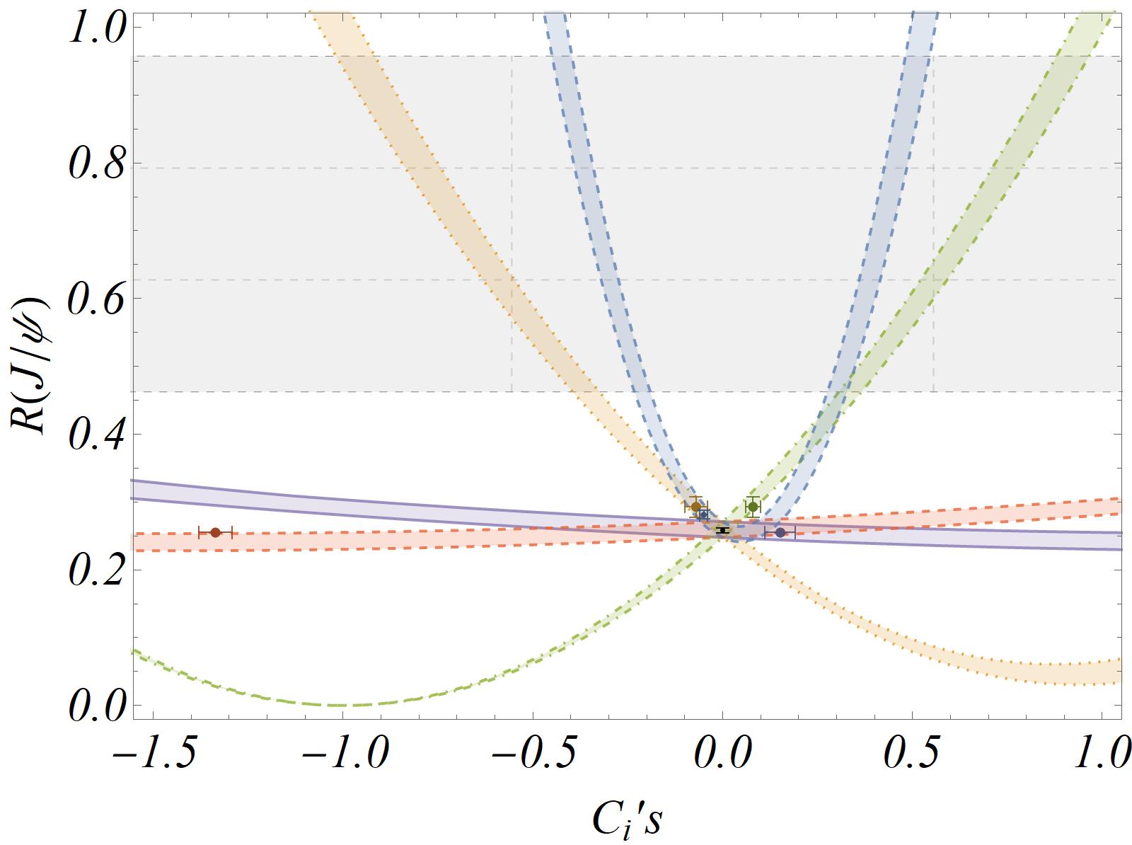
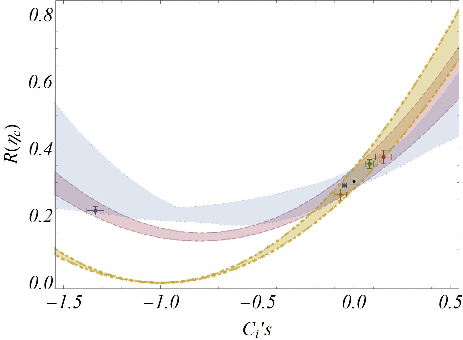
Figure 6: Variation of the $R(J/\psi)$ (top-left) and $R(\eta_{c})$ (top-right) observables w.r.t. real NP WC’s taken one at a time in the kinetic scheme. The grey regions are allowed by the current experimental limits, $R(J/\psi)^{expt.}$= $0.71(17)(18)$. In the plot, $R(J/\psi)^{SM}$=$0.2582(38)$ and $R(\eta_{c})^{SM}$=$0.302(10)$ and. Please consult the legend for the respective colour coding of the plots. The SM predictions and the predictions in the one operator scenarios are shown in dots with error bars. For the predictions please see the results of table 13.

		R(J/$\psi$)=$\frac{\Gamma(B_{c}^{-}\rightarrow J/\psi\tau^{-}\bar{\nu})}{\Gamma(B_{c}^{-}\rightarrow J/\psi\ell^{-}\bar{\nu})}(\ell=\mu,e)$	R($\eta_{c}$)=$\frac{\Gamma(B_{c}^{-}\rightarrow\eta_{c}\tau^{-}\bar{\nu})}{\Gamma(B_{c}\rightarrow\eta_{c}\ell^{-}\bar{\nu})}(\ell=\mu,e)$
Willson’s coefficients	best fit values	kinetic Scheme	kinetic Scheme
Re($C_{S_{1}}$)	0.152(40)	0.255(4)	0.373(24)
Re($C_{S_{2}}$)	-1.336(44)	0.240(4)	0.214(14)
Re($C_{V_{1}}$)	0.08(2)	0.301(12)	0.353(17)
Re($C_{V_{2}}$)	-0.07(3)	0.292(16)	0.262(19)
Re($C_{T}$)	-0.05(1)	0.281(8)	0.289(10)

Table 13: The NP sensitivities of $R(J/\psi)$ (third column) and $R(\eta_{c})$ (fourth column) for different one-parameter scenarios taken one at a time. The best fit points for the one parameter scenarios have taken from ref. Ray and Nandi (2023).

This section will discuss the NP effects in $B_{c}\to J/\psi(\eta_{c})\tau\nu_{\tau}$ decays. It was shown in ref. Ray and Nandi (2023) that the data on the decay rates and the angular distributions of $B\to D^{(*)}\mu(e)\nu$ decays suggest negligible NP effects in $b\to c\mu(e)\nu$ decays. Therefore, we have not considered the NP in $B_{c}\to J/\psi(\eta_{c})\mu\nu$ decays. The new operator basis for $b\to c\tau\nu_{\tau}$ decays is given by the following effective Hamiltonian

$${\cal H}_{eff} =\frac{4G_{F}}{\sqrt{2}}V_{cb}\left.[(\delta_{\ell\tau}+C_{V_{1}}^{\ell}){\cal O}_{V_{1}}^{\ell}+C_{V_{2}}^{\ell}{\cal O}_{V_{2}}^{\ell}+C_{S_{1}}^{\ell}{\cal O}_{S_{1}}^{\ell}+C_{S_{2}}^{\ell}{\cal O}_{S_{2}}^{\ell}+C_{T}^{\ell}{\cal O}_{T}^{\ell}\right.]\,,$$ (37)

where $C^{\ell}_{W}(W=V_{1},V_{2},S_{1},S_{2},T)$ are the new Wilson coefficients (WC) corresponding to the following four-fermi operators:

$${\cal O}_{V_{1}}^{\ell} =({\bar{c}}_{L}\gamma^{\mu}b_{L})({\bar{\tau}}_{L}\gamma_{\mu}\nu_{\ell L}),$$

$${\cal O}_{V_{2}}^{\ell} =({\bar{c}}_{R}\gamma^{\mu}b_{R})({\bar{\tau}}_{L}\gamma_{\mu}\nu_{\ell L}),$$

$${\cal O}_{S_{1}}^{\ell} =({\bar{c}}_{L}b_{R})({\bar{\tau}}_{R}\nu_{\ell L}),$$

$${\cal O}_{S_{2}}^{\ell} =({\bar{c}}_{R}b_{L})({\bar{\tau}}_{R}\nu_{\ell L}),$$

$${\cal O}_{T}^{\ell} =({\bar{c}}_{R}\sigma^{\mu\nu}b_{L})({\bar{\tau}}_{R}\sigma_{\mu\nu}\nu_{\ell L})\,.$$ (38)

Here, we have considered only left handed neutrinos. The decay distribution can be written as-

$$\frac{d\Gamma\left(B_{c}\rightarrow\eta_{c}\tau\overline{\nu}_{\tau}\right)}{dq^{2}}=\frac{G^{2}_{F}\left|V_{cb}\right|^{2}}{192\pi^{3}m^{3}_{B_{c}}}q^{2}\sqrt{\lambda_{\eta_{c}}(q^{2})}\left(1-\frac{m^{2}_{\tau}}{q^{2}}\right)^{2}\left\{\left|1+C_{V_{1}}+C_{V_{2}}\right|^{2}\left[\left(1+\frac{m^{2}_{\tau}}{2q^{2}}\right)H^{s2}_{V,0}+\frac{3}{2}\frac{m^{2}_{\tau}}{q^{2}}H^{s2}_{V,t}\right]\right.$$

$$~{}~{}~{}\left.+\frac{3}{2}\left|C_{S_{1}}+C_{S_{2}}\right|^{2}H^{s2}_{S}+8\left|C_{T}\right|^{2}\left(1+\frac{2m^{2}_{\tau}}{q^{2}}\right)H^{s2}_{T}+3\mathcal{R}e\left[\left(1+C_{V_{1}}+C_{V_{2}}\right)\left(C^{*}_{S_{1}}+C^{*}_{S_{2}}\right)\right]\frac{m_{\tau}}{\sqrt{q^{2}}}H^{s}_{S}H^{s}_{V,t}\right.$$

$$~{}~{}~{}\left.-12\mathcal{R}e\left[\left(1+C_{V_{1}}+C_{V_{2}}\right)C^{*}_{T}\right]\frac{m_{\tau}}{\sqrt{q^{2}}}H^{s}_{T}H^{s}_{V,0}\right\}\,,$$ (39)

and

$$\frac{d\Gamma\left(B_{c}\rightarrow J/\psi\tau\overline{\nu}_{\tau}\right)}{dq^{2}}=\frac{G^{2}_{F}\left|V_{cb}\right|^{2}}{192\pi^{3}m^{3}_{B_{c}}}q^{2}\sqrt{\lambda_{J/\psi}(q^{2})}\left(1-\frac{m^{2}_{\tau}}{q^{2}}\right)^{2}\left\{\left(\left|1+C_{V_{1}}\right|^{2}+\left|C_{V_{2}}\right|^{2}\right)\left[\left(1+\frac{m^{2}_{\tau}}{2q^{2}}\right)\left(H^{2}_{V,+}+H^{2}_{V,-}+H^{2}_{V,0}\right)\right.\right.$$

$$~{}~{}~{}\left.\left.+\frac{3}{2}\frac{m^{2}_{\tau}}{q^{2}}H^{2}_{V,t}\right]-2\mathcal{R}e\left[\left(1+C_{V_{1}}\right)C^{*}_{V_{2}}\right]\left[\left(1+\frac{m^{2}_{\tau}}{2q^{2}}\right)\left(H^{2}_{V,0}+2H_{V,+}H_{V,-}\right)+\frac{3}{2}\frac{m^{2}_{\tau}}{q^{2}}H^{2}_{V,t}\right]+\frac{3}{2}\left|C_{S_{1}}-C_{S_{2}}\right|^{2}H^{2}_{S}\right.$$

$$~{}~{}~{}\left.+8\left|C_{T}\right|^{2}\left(1+\frac{2m^{2}_{\tau}}{q^{2}}\right)\left(H^{2}_{T,+}+H^{2}_{T,-}+H^{2}_{T,0}\right)+3\mathcal{R}e\left[\left(1+C_{V_{1}}-C_{V_{2}}\right)\left(C^{*}_{S_{1}}-C^{*}_{S_{2}}\right)\right]\frac{m_{\tau}}{\sqrt{q^{2}}}H_{S}H_{V,t}\right.$$

$$\left.-12\mathcal{R}e\left[\left(1+C_{V_{1}}\right)C^{*}_{T}\right]\frac{m_{\tau}}{\sqrt{q^{2}}}\left(H_{T,0}H_{V,0}+H_{T,+}H_{V,+}-H_{T,-}H_{V,-}\right)\right.$$

$$~{}~{}~{}\left.+12\mathcal{R}e\left[C_{V_{2}}C^{*}_{T}\right]\frac{m_{\tau}}{\sqrt{q^{2}}}\left(H_{T,0}H_{V,0}+H_{T,+}H_{V,-}-H_{T,-}H_{V,+}\right)\right\}\,.$$ (40)

In Fig. 6, we depict the variations of $R(J/\psi)$ and $R(\eta_{c})$ w.r.t the various NP WCs. Note that corresponding to the scalar operators, one observes only a slight variation in $R(J/\psi)$ while it could be relatively large in $R(\eta_{c})$. However, the deviations from the respective SM predictions could be significant in both scenarios with additional left or right-handed or tensor quark operators. Experimental measurement is available for $R(J/\psi)$ and is provided in eq. 1. It is represented by the grey region in the top-left plot in fig. 6. Note that the data is a few sigma away from the respective SM predictions. The one-operator scenarios with a scalar operator cannot explain the data. However, the one operator scenarios $\mathcal{O}_{V_{1}}$ or $\mathcal{O}_{V_{2}}$ or $\mathcal{O}_{T}$ can. We have also checked whether the NP allowed by $R(D^{(*)})$ in the semileptonic $B\to D^{(*)}$ decays can explain the present data on $R(J/\psi)$. To check this, we have taken the constraints on the new WCs from ref. Ray and Nandi (2023), which is based on the data on $R(D^{(*)})$. The respective values obtained for $R(J/\psi)$ are shown in table 13. These estimates are also indicated in the figure. For details, please check the legend. As can be noted, the available constraints on the new real WCs are not consistent with the observation on $R(J/\psi)$. None of the scenarios can explain the $R(J/\psi)$ data. However, we do observe deviations from the SM prediction. In a similar fashion, we obtain the values for $R(\eta_{c})$ corresponding to the allowed values of the new WCs, which are shown in table 13 and in the top-right plot in Fig. 6. We also register deviations w.r.t the SM prediction. For a check, precise measurements of both these observables are necessary.

IV A few non-leptonic decays of $B_{c}$ meson into charmonium:

Non-leptonic decays of heavy mesons offer an opportunity to understand the nature of Quantum Chromodynamics(QCD). The $B_{c}$ mesons can decay non-leptonically via the decays of the $\bar{b}$ quark with the c quark as the spectator or vice versa. There could also be annihilation dominated decays of $B_{c}$ mesons. We study the exclusive non-leptonic two-body $B_{c}$ decays within the factorization approximation with the leading order non-factorizable corrections calculated in NRQCD Qiao et al. (2014); Zhu et al. (2017); Zhu (2018). As a leading order approximation, naive factorization is widely used to study these decays in which the non-leptonic decay amplitudes reduce to the product of the form factor and a decay constant. For the decays we have considered in this analysis, the amplitudes are expressed as the product of the decay constant and the transition form factors for $B_{c}\to J/\psi(\eta_{c})$ transitions. For the decay constant, we have used the corresponding lattice estimates Zyla et al. (2020a) and the lattice estimates for the relevant form factors in $B_{c}\to J/\psi$ decays. At the same time, for $f_{+,0}^{B_{c}\to\eta_{c}}$ we use our estimates given in the subsection III.1. In evaluating the non-factorizable corrections, we have used our estimates for radial wave functions given in table 7. The branching fractions of a few such non-leptonic decays have been measured.

Figure 7: Tree level Feynman diagrams for the non-leptonic $B_{c}\to(c\bar{c})(P,V)$ decays, where P and V stand for a light pseudo-scalar meson and a vector meson and (c$\bar{c}$) stands for S and P wave charmonium.

IV.0.1 Formalism

The theoretical description of the non-leptonic decays involves the matrix elements of the local four-fermion operators. The effective and CKM favored Hamiltonian for the $b\to c\bar{u}d$ transition can be written as follows:

$$\mathcal{H}_{eff}=\frac{G_{F}}{\sqrt{2}}V^{*}_{ud}V_{cb}\big{(}C_{1}(\mu)Q_{1}(\mu)+C_{2}(\mu)Q_{2}({\mu})\big{)},$$ (41)

Here, $V_{ud}$, $V_{cb}$ are the CKM matrix elements, and the $C_{i}({\mu})$s are the Wilson coefficients (WCs) which take into account the short-distance effects. The WCs $C_{1,2}(\mu)$ are evaluated perturbatively at the W scale and are then evolved down to the renormalization scale $\mu\approx m_{b}$ by the renormalization group equations. The effects of soft gluons below the scale $\mu$ with the virtualities remain in the hadronic matrix elements of the local four-fermion operators $Q_{i}$. The four-fermion effective operators $Q_{1,2}(\mu)$ are defined as

$$Q_{1} =\bar{d}_{\alpha}\gamma^{\mu}(1-\gamma_{5})u_{\alpha}\bar{c}_{\beta}\gamma_{\mu}(1-\gamma_{5})b_{\beta},$$

$$Q_{2} =\bar{d}_{\alpha}\gamma^{\mu}(1-\gamma_{5})u_{\beta}\bar{c}_{\beta}\gamma_{\mu}(1-\gamma_{5})b_{\alpha},$$ (42)

where $\alpha$ and $\beta$ are color indices, and the summation conventions over repeated indices are understood. The Fierz rearrangement

$$T^{A}_{\alpha\beta}T^{A}_{\rho\lambda}=-\frac{1}{6}\delta_{\alpha\beta}\delta_{\rho\lambda}+\frac{1}{2}\delta_{\alpha\lambda}\delta_{\rho\beta},$$ (43)

can be used to change the above basis to

$$Q_{0}=Q_{1},~{}~{}~{}~{}Q_{8}=-\frac{1}{6}Q_{1}+\frac{1}{2}Q_{2},$$ (44)

with the following Wilson coefficients (WCs) Buchalla et al. (1996)

$$C_{0}=C_{1}+C_{2}/3=\frac{2}{3}C_{+}+\frac{1}{3}C_{-}\,,~{}~{}C_{8}=2C_{2}=C_{+}-C_{-}\,,$$ (45)

where

$$C_{\pm}=\left[\frac{\alpha_{s}(M_{W})}{\alpha_{s}(\mu)}\right]^{\frac{\gamma_{\pm}}{2\beta_{0}}}\,,~{}~{}\gamma_{\pm}=\pm 6\frac{N_{c}\mp 1}{N_{c}}\,,~{}~{}\beta_{0}=\frac{11N_{c}-2n_{f}}{3}\,.$$ (46)

In this paper, we have only focused on the CKM favored processes. Here, we do not consider non-leptonic $B_{c}$ decays into $D^{(*)},$ $D_{s}^{(*)}$ mesons as these decays are strongly CKM suppressed. We limit our analysis of the $B_{c}$ non-leptonic decays to the case when the final meson $M_{c\bar{c}}$ is charmonium, and the light $M$ meson is $\pi$, $K^{(*)}$, $\rho$. The corresponding Feynman diagram is shown in fig 7.

Gegenbauer Coefficients			Decay constant	Form factors
Mesons	Coefficient	Values	(MeV) Zyla et al. (2020a)	(Kin. sch.)
$\pi$ Bali et al. (2019)	$a_{1}$	$0$	$f_{\pi}=130.5$	$f_{0}(m_{\pi}^{2})=0.505(44)$
	$a_{2}$	$0.116^{+19}_{-20}$
$K$ Bali et al. (2019)	$a_{1}$	$0.0525^{+31}_{-33}$	$f_{K}=155.72$	$f_{0}(m_{K}^{2})=0.510(44)$
	$a_{2}$	$0.106^{+15}_{-16}$
	$a_{1}^{||,\perp}$	0
$\rho$ Braun et al. (2017)	$a_{2}^{||}$	$0.132\pm 0.027$	$f_{\rho}=221$	$f_{+}(m_{\rho}^{2})=0.527(44)$
	$a_{2}^{\perp}$	$0.101\pm 0.022$
	$a_{1}^{||}$	$0.03\pm 0.02$
$K^{*}$ Ball and Jones (2007)	$a_{1}^{\perp}$	$0.04\pm 0.03$	$f_{K^{*}}=220$	$f_{+}(m_{K^{*}}^{2})=0.534(44)$
	$a_{2}^{||}$	$0.11\pm 0.09$
	$a_{2}^{\perp}$	$0.10\pm 0.08$

Table 14: Gegenbauer moments for the twist-2 distribution amplitudes of light mesons and the inputs for the decay constants used in the estimate of the branching fractions of the non-leptonic decays of $B_{c}$ meson.

Following the naive-factorization approximation the amplitude can be expressed as

$$\langle M_{c\bar{c}}M|\mathcal{H}_{eff}|B_{c}\rangle\propto C_{i}\langle M_{c\bar{c}}|(\bar{b}c)_{V-A}|B_{c}\rangle\times\langle M|(\bar{q_{1}}q_{2})_{V-A}|0\rangle\approx C_{i}f_{M}F^{B_{c}\to M_{c\bar{c}}},$$ (47)

where $f_{M}$ and $F^{B_{c}\to M_{c\bar{c}}}$ are the decay constant and the form factor, respectively. Note that in the above equation, the matrix elements of the weak current between the vacuum and a pseudoscalar (P) or a vector (V) meson have been parametrized by the decay constant $(f_{P},f_{V})$ and defined as:

$$\langle P(p_{\mu})|{(\bar{q_{1}}q_{2})}_{V-A}|0\rangle=-if_{P}p_{\mu},~{}~{}~{}\\ \langle V|{(\bar{q_{1}}q_{2})}_{V-A}|0\rangle=-if_{V}m_{V}\epsilon^{*}_{\mu},$$

where $m_{V}$ and $\epsilon_{\mu}$ are the mass and polarization vectors of the vector meson. The matrix elements $\langle M_{c\bar{c}}|(\bar{b}c)_{V-A}|B_{c}\rangle$ are already defined in eq. II.1. Note that, in general the matrix element between the vacuum and the mesonic state can be parametrized by the mesonic wave function and its decay constant as follows:

$$\langle 0|q_{1}(0)\gamma^{\mu}\gamma_{5}q_{2}(0)|P(P)\rangle =if_{P}P^{\mu}\int_{0}^{1}dx\phi_{P}(x),$$ (48)

$$\langle 0|q_{1}(0)\gamma^{\mu}q_{2}(0)|V(P),\epsilon_{\lambda=0}\rangle =if_{V}M_{V}\epsilon^{\mu}\int_{0}^{1}dx\phi_{V\parallel}(x),$$ (49)

$$\langle 0|q_{1}(0)\sigma^{\mu\nu}q_{2}(0)|V(P),\epsilon_{\lambda=\pm 1}\rangle =if_{V}^{\perp}\int_{0}^{1}dx(\epsilon^{\mu}P^{\nu}-\epsilon^{\nu}P^{\mu})~{}\phi_{V\perp}(x).$$ (50)

Hence, following the QCD factorization approach, the most general expression for the decay amplitude for $B_{c}\to M_{1}(c\bar{c})M_{2}$ decays is given by

$${\cal A}(B_{c}\to M_{1}(c\bar{c})M_{2})\sim F^{B\to M_{1}}(0)f_{M_{2}}\int_{0}^{1}{dx\ T_{H}(x)\ \phi_{M_{2}}}(x)+\mathcal{O}(\frac{1}{m_{b}})+\mathcal{O}(v^{2}),$$ (51)

where $F^{B\to M_{1}}$ and $f_{M_{2}}$ are the form factor and the decay constant, respectively. $M_{1}$ represents the meson that takes away the spectator quark. $\phi_{M_{2}}$ is the light-cone-distribution amplitude (LCDA) of the meson $M_{2}$, and the $T_{H}$ are the perturbatively calculable hard-scattering kernels for the various operators in the effective weak Hamiltonian (eq. 41 ). In the naive factorization approximation, $T_{H}$ is independent of $x$, and $\int_{0}^{1}{dx\ \phi_{M_{2}}}(x)=1$ is obtained from the normalization. Hence, under this approximation, the amplitude is proportional to the product of the decay constant and the form factor. Once we add the non-factorizable contributions, i.e. contributions from the diagrams containing gluon exchanges that do not belong to the form factor for the $B_{c}\to M_{1}$ transition, the hard scattering kernels given in eq. 51 can be generalized as Qiao et al. (2014),

$${\cal A}(B_{c}^{+}\to J/\psi(\eta_{c})P)=\frac{G_{F}}{\sqrt{2}}V_{ud}^{*}V_{cb}\int_{0}^{1}{dx\ \phi_{P}(x)\Big{[}C_{0}(\mu)\big{(}T_{f,0}(\mu)+T_{nf,0}(x,\mu)\big{)}\langle Q_{0}\rangle+C_{8}(\mu)T_{nf,8}(x,\mu)\langle Q_{8}\rangle\Big{]}},$$ (52)

$$T_{f,i}(\mu)=\sum_{k=0}^{\infty}(\frac{\alpha_{s}}{4\pi})^{k}T^{(k)}_{f,i}(\mu)\,,~{}~{}~{}T_{nf,i}(\mu)=\sum_{k=0}^{\infty}(\frac{\alpha_{s}}{4\pi})^{k}T^{(k)}_{nf,i}(\mu)\,,$$ (53)

where $P$ is a pseudoscalar meson. In these equations, the hard kernels $T_{f}$ and $T_{nf}$ represent the factorizable and non-factorizable contributions in the decay amplitudes, respectively, which are perturbatively calculable. These can further be classified as the contributions to $\langle Q_{0}\rangle$ and $\langle Q_{8}\rangle$, respectively. In NRQCD, the matrix elements $\langle Q_{0}\rangle$ and $\langle Q_{8}\rangle$ for $B_{c}\to\eta_{c}$ decays can be written as Qiao et al. (2014):

Decay modes	Kinetic Scheme		Other estimates
$(\times 10^{3})$	Naive Fac.	with corrections	PQCD	RQM	QCDSR
		(fac. + Non-fact. (LO))	Rui and Zou (2014)	Ebert et al. (2003b)	Kiselev (2002)
$\mathcal{B}(B_{c}\to\text{J/$\psi\pi$})$	0.703(92)	0.698(92)	$2.33(63)$	$0.61$	$1.3$
$\mathcal{B}(B_{c}\to\text{J/$\psi$K})$	0.053(7)	0.053(7)	$0.19(4)$	$0.05$	$0.11$
$\mathcal{B}(B_{c}\to\eta_{c}\pi)$	0.855(119)	0.840(118)	$2.98(84)$	$0.85$	$2.0$
$\mathcal{B}(B_{c}\to\eta_{c}K)$	0.065(9)	0.064(9)	$0.24(4)$	$0.07$	$0.13$
$\mathcal{B}(B_{c}\to\eta_{c}\rho)$	2.422(324)	2.380(321)	$9.83(138)$	$2.1$	$4.2$
$\mathcal{B}(B_{c}\to\eta_{c}K^{*})$	0.127(17)	0.125(17)	$0.57(10)$	$0.11$	$0.20$

Table 15: The predictions for the branching fractions in a few $B_{c}\to\eta_{c}(P,V)$, and $B_{c}\to J/\psi P$ decays. For the predictions with non-factorizable corrections the radial wave functions are taken from Fit-III of table 7. Our predictions have been compared with those obtained in other methods/models.

$$\langle Q_{0}\rangle^{B_{c}\to\eta_{c}P}= (M_{B_{c}}^{2}-M_{\eta_{c}}^{2})f_{P}f^{B_{c}\to\eta_{c}}_{0}(q^{2}=M_{P}^{2})$$ (54)

$$\langle Q_{8}\rangle^{B_{c}\to\eta_{c}P}= \frac{2\sqrt{2}\pi f_{P}\psi_{\eta_{c}}(0)\psi_{B_{c}}(0)C_{A}C_{F}\alpha_{s}\sqrt{m_{b}+m_{c}}(m_{b}+3m_{c})^{2}(xm_{c}-(x-1)m_{b})}{m_{c}^{3/2}N_{c}^{2}(m_{c}-m_{b})\big{(}(x-1)m_{b}+(3x-2)m_{c}\big{)}\big{(}xm_{b}+(3x-1)m_{c}\big{)}}.$$

The same matrix elements for $B_{c}\to J/\psi$ decays are obtained as Qiao et al. (2014)

$$\langle Q_{0}\rangle^{B_{c}\to J/\psi P}= -2m_{J/\psi}f_{P}P_{B_{c}}\cdot\epsilon^{*}_{J/\psi}A_{0}^{B_{c}\to\eta_{c}}(q^{2}=M_{P}^{2})$$ (55)

$$\langle Q_{8}\rangle^{B_{c}\to J/\psi P}=- \frac{8\sqrt{2}\pi f_{P}\psi_{J/\psi}(0)\psi_{B_{c}}(0)P_{B_{c}}\cdot\epsilon^{*}_{J/\psi}C_{A}C_{F}\alpha_{s}(m_{b}+m_{c})^{2}}{m_{c}^{1/2}N_{c}^{2}(m_{b}-m_{c})^{2}\big{(}(x-1)m_{b}+(3x-2)m_{c}\big{)}\big{(}xm_{b}+(3x-1)m_{c}\big{)}}\times$$

$$\bigg{(}3(2x-1)m_{b}m_{c}+(x-1)m_{b}^{2}+(9x-4)m_{c}^{2}\bigg{)}.$$

Here, $\psi_{c\bar{c}}(0)$ and $\psi_{M_{2}}(0)$ are the Schrödinger wave function defined earlier. In the above equations, we define $P_{B_{c}}\cdot\epsilon^{*}_{J/\psi}=\frac{m_{B_{c}}}{m_{J/\psi}}|p|$, $|p|=\frac{\sqrt{[m_{B_{c}}^{2}-(m_{J/\psi}+m_{p})^{2}][m_{B_{c}}^{2}-(m_{J/\psi}-m_{p})^{2}]}}{2m_{B_{c}}}$, $z=\frac{m_{c}}{m_{b}}$, $m_{B_{c}}=(m_{b}+m_{c})$, $m_{J/\psi}=m_{\eta_{c}}=2m_{c}$. In the above expressions, we have used the inputs on the form factors extracted from lattice discussed earlier. Note that at the tree level, the hard kernel $T_{f,0}^{0}=1$ and independent of $x$. At the one-loop level $T_{f,0}^{1}(\mu)$ does not depend on $x$ either. For these types of contributions the convolution integral in eq. IV.0.1 could simply be written as $\int_{0}^{1}{dx\ \phi_{P}(x)}=1$, the normalization condition. At the lowest order for both the decay modes $T_{nf,0}^{0}=0$ and $T_{nf,8}^{0}=1$. The detailed mathematical expressions for the $T_{f,0}^{1}$, $T_{nf,0}^{1}$ and $T_{nf,8}^{1}$ can be obtained from ref. Qiao et al. (2014). However, we have not taken into account the non-factorizable contributions $T_{nf,0}^{1}$ and $T_{nf,8}^{1}$ in our analysis. The LCDA of light meson can be written as an expansion in Gegenbauer polynomials, defined as follows:

$$\phi_{M}(x,\mu^{2})=6x(1-x)\big{[}1+\sum_{n=1}^{\infty}a_{n}^{M}(\mu^{2})C_{n}^{3/2}(2x-1)\big{]},$$ (56)

where the Gegenbauer polynomial is given by the coefficient $C_{n}^{3/2}(2x-1)$ and $a_{n}^{M}$s are the Gegenbauer moments. In the asymptotic limit, the above equation can be written as $\phi_{M}(x)\approx 6x(1-x)$. Following the definitions given in eq. 48 we obtain that only the parallel component of the wave functions contributes to the decay amplitude in $B_{c}\to\eta_{c}V(\rho,K^{*})$ decays. The transition amplitude for $B_{c}\to\eta_{c}V$ will have only the longitudinal components $\mathcal{A}_{||}$ which can be expressed as

$$\mathcal{A}_{||}(B_{c}\to\eta_{c}~{}V) =\frac{G_{F}}{\sqrt{2}}V_{ud}^{*}V_{cb}\int_{0}^{1}dx\ \phi_{V,||}(x)\times$$

$$\biggl{(}C_{0}(\mu)\big{(}T_{f,0}(\mu)+T_{nf,0}(x,\mu)\big{)}\langle Q_{0}\rangle^{B_{c}\to\eta_{c}V}+C_{8}(\mu)T_{nf,8}(x,\mu)\langle Q_{8}\rangle^{B_{c}\to\eta_{c}V}\biggr{)},$$

with the twist-2 LCDA given by

$$\phi_{V,||}(x,\mu)=6x(1-x)\big{[}1+\sum_{n=1}^{\infty}a_{n,||}(\mu)C_{n}^{3/2}(2x-1)\big{]},$$ (57)

The matrix elements $\langle Q_{0}\rangle^{B_{c}\to\eta_{c}V}$ and $\langle Q_{8}\rangle^{B_{c}\to\eta_{c}V}$ can be obtained from eq. 54 with the replacement $f_{P}\to f_{V}$. In this analysis, we will predict the branching fractions of the $B_{c}\to J/\psi(\pi,K)$ and $B_{c}\to\eta_{c}(\pi,K,K^{*},\rho)$ decays. The available inputs on the Gegenbauer moments are given in table 14 which we have used in our analysis.

Following the formalism and the relevant inputs discussed above, we have predicted the respective branching fractions. We have presented the results in the naive factorization approximation and including non-factorizable corrections at LO (discussed above), respectively. As discussed before, for the numerical estimates we need the inputs on the form factors $A_{0}^{B_{c}\to J/\psi}(M_{P}^{2})$ and $f_{0}^{B_{c}\to\eta_{c}}(M_{P}^{2})$ where $M_{p}$ is the mass of the light meson to which $B_{c}$ is decaying. Following are the lattice inputs for $A_{0}$ and $f_{0}$:

$$A_{0}^{B_{c}\to J/\psi}(m_{\pi}^{2})=0.478\pm 0.031,\ \ \ \ f_{0}^{B_{c}\to\eta_{c}}(m_{K}^{2})=0.513\pm 0.035,$$ (58)

which we have extracted from the results of ref. Harrison et al. (2020a). The inputs for the $f_{0}$’s are shown in table 14, which we have obtained from our analysis in subsection III.1. In this table, we have presented the results in the kinetic scheme. For the numerical estimates of the non-factorizable corrections calculated in NRQCD, we need inputs on the radial wave functions which we have taken from “Fit-III” of table 7. The inputs on Gegenbauer coefficients for the light meson wave functions have been taken from table 14.

Using all the relevant inputs discussed above, we predict the respective branching fractions shown in table 15. The estimated errors in the branching fractions in both estimates are $\approx$ 15%. This precision is based on lattice inputs. We have compared our results with other estimates based on QCD models. In PQCD Rui and Zou (2014) and QCDSR Ebert et al. (2003b) approaches, the estimated values are relatively higher due to the different inputs for the form factors used in both analyses. However, our predictions include the estimates presented in the relativistic quark model Kiselev (2002), though they have not provided any error in their estimates. We have estimated the $f_{0}(M_{P}^{2})$ in the other two mass schemes, which are shown in table 19 (appendix). Using these inputs alongside other inputs discussed above, we obtain the predictions for the branching fractions shown in the appendix in table 20. These predictions are consistent with those obtained in the kinetic scheme.

V Predictions for other production and decay modes for Charmonium

Using the results in table 7, one could update the predictions of various decay rates and production or annihilation cross-sections calculated in the NRQCD effective theory involving these charmoniums. This is not the goal of this paper. However, we update the predictions of a few interesting channels in this section.

V.1 Electron positron annihilation to charmonium:

We have also studied $e^{+}e^{-}$ decays into double charmonium in the scope of the NRQCD framework. The corresponding results are presented below in table 16. The explicit expressions for the cross-sections corresponding to these decay channels are presented below.

• $e^{+}e^{-}\rightarrow J/\psi+\eta_{c}$:
  The production rate up to $\mathcal{O}(\alpha_{s}v^{2})$ can be written as Dong et al. (2012); Li and Wang (2014).

  $$\sigma[e^{+}e^{-}\rightarrow J/\psi+\eta_{c}]=\sigma_{0}+\sigma_{2}+\mathcal{O}(\sigma_{0}v^{4})$$ (59)

  Where,

  $$\sigma_{0}=\frac{8\pi\alpha^{2}m_{c}^{2}(1-4r)^{3}/2}{3}\langle\mathcal{O}_{1}\rangle_{J/\psi}\langle\mathcal{O}_{1}\rangle_{\eta_{c}}|c_{0}|^{2}$$ (60)

  $$\sigma_{2}= \frac{4\pi\alpha^{2}m_{c}^{2}(1-4r)^{3}/2}{3}\langle\mathcal{O}_{1}\rangle_{J/\psi}\langle\mathcal{O}_{1}\rangle_{\eta_{c}}\biggl{\{}\bigg{(}\frac{1-10r}{1-4r}|c_{0}|^{2}+4Re[c_{0}c^{*}_{2,1}]\bigg{)}\langle v^{2}\rangle_{J/\psi}$$ (61)

  $$+(\frac{1-10r}{1-4r}|c_{0}|^{2}+4Re[c_{0}c^{*}_{2,2}]\bigg{)}\langle v^{2}\rangle_{\eta_{c}}\biggr{\}}$$ (62)

  where $c_{0},c_{2,1},c_{2,2}$ are given in ref Dong et al. (2012); Li and Wang (2014). The measured values of this cross section by the BaBar collaboration is given by Aubert et al. (2005)

  $$\sigma[e^{+}e^{-}\rightarrow J/\psi+\eta_{c}]=17.03\pm 1.2~{}\text{fb},$$ (63)

  while that from the Belle collaboration Abe et al. (2002, 2004) is

  $$\sigma[e^{+}e^{-}\rightarrow J/\psi+\eta_{c}]=24.6\pm 2.8(\text{stat.})\pm 3.4(\text{syst.})~{}\text{fb}.$$ (64)

Decay Channel	$\mu$	Cross-section(fb)	Cross-section(fb)	Cross-section(fb)
		Kin.	$\overline{\bf MS}$. Scheme	Pol. Scheme
$\sigma(e^{+}e^{-}\to J/\psi\eta_{c})$	$2m_{c}$	$25.094(2029)$	$24.619(1903)$	$26.700(2197)$
$\sigma(e^{+}e^{-}\to J/\psi\eta_{c})$	$\frac{\sqrt{s}}{2}$	$19.139(1549)$	$22.507(1740)$	28.806(2370)
$\sigma(e^{+}e^{-}\to\eta_{c}\gamma)$	$\frac{\sqrt{s}}{2}$	$39.527(3015)$	$40.573(3053)$	44.427(3409)

Table 16: Cross section estimates for $e^{+}e^{-}$ decays into double charmonium.

• $e^{+}e^{-}\rightarrow\eta_{c}\gamma$

An electromagnetic transition between quarkonium states offers the distinctive experimental signature of a monochromatic photon, a useful production mechanism for discovery and study of the lower-lying state, and a unique window on the dynamics of such systems. In this regard, we predict the scattering cross section $\sigma(e^{+}e^{-}\to\eta_{c}\gamma)$ using our result. The corresponding expression for the cross-section including the available corrections at order $\alpha_{s}$, $v^{2}$ and $\alpha_{s}v^{2}$ is given by  Xu et al. (2014)

$$\sigma=\hat{\sigma}^{(0)}_{\eta_{c}}\big{[}1+\alpha_{s}c^{10}+(c^{02}+\alpha_{s}c^{12})\langle v^{2}\rangle\big{]}\langle 0|\mathcal{O}^{H}|0\rangle,$$ (65)

where the LO short-distance cross section for $\eta_{c}$ is given by

$$\hat{\sigma}^{(0)}_{\eta_{c}}=\frac{(4\pi\alpha)^{3}Q_{c}^{4}(1-r)}{6\pi m_{c}s^{2}}.$$ (66)

The analytical expressions for the asymptotic behaviour of $c^{02}$, $c^{10}$ and $c^{12}$ at high energies ($r\to 0$) are taken from ref. Xu et al. (2014), which are as follows

$$\lim\limits_{r\rightarrow 0}c^{02} = -\frac{5}{6}$$

$$\lim\limits_{r\rightarrow 0}c^{10} = -\frac{2}{9\pi}[3(3-2\ln 2)\ln r+9(\ln^{2}2-3\ln 2+3)+\pi^{2}]$$ (67)

$$\approx -0.34\ln r-1.59$$

$$\lim\limits_{r\rightarrow 0}c^{12} = \frac{1}{27\pi}[3(21-10\ln 2)\ln r+15(3\ln^{2}2-7\ln 2)+28+5\pi^{2}]$$

$$\approx 0.50\ln r+0.31$$

The LO long-distance matrix elements are obtained from the radial wave functions at the origin:

$$\langle 0|\mathcal{O}^{\eta_{c}(nS)}|0\rangle = \frac{2N_{c}|\psi_{\eta_{c}}^{R}(0)|^{2}}{4\pi}$$ (68)

Using the results obtained on $\psi_{\eta_{c}}^{R}(0)$, we have obtained the following result,

$$\sigma(e^{+}e^{-}\text{$\to$ }\eta_{c}\text{ $\gamma$})=(39.527\pm 3.015)\ \text{fb},$$ (69)

which is consistent with the result available in ref. Xu et al. (2014),

$$\sigma(e^{+}e^{-}\text{$\to$ }\eta_{c}\text{ $\gamma$})=(54\pm 15)\ \text{fb}.$$ (70)

We provide our estimates for the production cross-sections of S-wave charmonia in table 16.

V.2 Z boson decays into charmonium

Decay Modes	Kin.	$\overline{\bf MS}$	Pol.
$10^{12}\times\mathcal{B}(Z\to\eta_{c}+J/\psi)$ Likhoded and Luchinsky (2018)	0.0573(46)	0.0865(67)	0.210(17)
$10^{12}\times\mathcal{B}(Z\to J/\psi$+$J/\psi)$ Luchinsky (2017)	0.0670(21)	0.0984(21)	0.2312(77)
$10^{8}\times\mathcal{B}(\text{$Z\to\eta_{c}+\gamma$})$ Luchinsky (2017)	1.169(89)	1.252(94)	1.51(12)
$10^{8}\times\mathcal{B}(\text{$Z\to J/\psi+\gamma$})$  Luchinsky (2017)	10.96(17)	11.46(12)	13.32(22)

Table 17:

Using our results for the radial wave functions we have updated the rates of various $Z$ decays involving charmonium final states. These include radiative decays including $J/\psi$ or $\eta_{c}$ in the final state. Equally important channels are the exclusive $Z$ boson decays into charmonium-charmonium final states. We have updated the decay rates calculated at the leading order in NRQCD Likhoded and Luchinsky (2018); Luchinsky (2017). The corresponding expressions are given by

$$\Gamma(Z\rightarrow\gamma\eta_{c})=\frac{2\alpha c_{V}^{2}e_{c}^{2}\tilde{f}_{\eta_{c}}^{2}}{3M_{Z}}(1-4r^{2})$$ (71)

$$\Gamma(Z\rightarrow\gamma J/\psi)=\frac{2\alpha c_{A}^{2}e_{c}^{2}\tilde{f}_{J/\psi}^{2}}{3M_{Z}}(1-16r^{4})$$ (72)

and

$$\Gamma(Z\to\eta_{c}J/\psi) = \frac{8192\pi\alpha_{s}^{2}\beta^{3}c_{V}^{2}\tilde{f}_{\eta_{c}}^{2}\tilde{f}_{J/\psi}^{2}r^{2}}{243M_{Z}^{3}}$$ (73)

$$\Gamma(Z\to J/\psi J/\psi) = \frac{1024\pi\alpha_{s}^{2}\beta^{5}c_{A}^{2}\tilde{f}_{J/\psi}^{4}r^{2}}{243M_{Z}^{3}}.$$ (74)

where $r=\frac{m_{c}}{M_{Z}}$. The NRQCD constants $\tilde{f_{Q}}$ are defined as

$$\tilde{f}_{\eta_{c}}=\tilde{f}_{J/\psi}=\sqrt{\frac{\langle\mathcal{O}_{1}\rangle_{J/\psi}}{m_{c}}}.$$ (75)

We provide numerical predictions for the BRs of Z boson decays to di-charmonium final states and radiative decays of Z boson into charmonium final states, which are presented in table 17. The inputs on the radial wave functions for $J/\psi$ and $\eta_{c}$ mesons are taken from table 7.This is the first numerical analysis that provides the predictions with the corresponding 1$\sigma$ CI. The earlier numerical analyses Likhoded and Luchinsky (2018); Luchinsky (2017) do not provide any error. However, our estimates within the 1$\sigma$ CI’s include the estimated number in these publications. An objective statistical comparison with the existing literature is currently impossible since most of the corresponding references do not estimate the related uncertainties.

VI Summary

This paper discusses the semileptonic and nonleptonic decays of the $B_{c}$ meson to S-wave charmonia, like the $J/\psi$ and $\eta_{c}$ mesons. In this analysis, we use the available lattice inputs on the $B_{c}\to J/\psi$ form factors and the branching fractions: $\mathcal{B}(J/\psi\to e^{+}e^{-})$, $\mathcal{B}(J/\psi\to 3\gamma)$ and $\mathcal{B}(\eta_{c}\to 2\gamma)$. Using lattice inputs on the form factors and HQSS, we extract the shapes of the form factors $f_{+,0}^{B_{c}\to\eta_{c}}(q^{2})$. We also extract the Isgur-Wise function defined at the zero recoil ($q^{2}_{max}$) in $B_{c}\to J/\psi(\eta_{c})$ transitions and the parameters related to the symmetry-breaking effects at the non-zero recoils in the process. We have extracted all these parameters in a statistically consistent way. Using these form factors we have predicted the $q^{2}$ integrated branching fractions $\mathcal{B}(B_{c}^{-}\to\eta_{c}\tau^{-}(\mu^{-})\bar{\nu})$ and the LFU ratio of the rates $R(\eta_{c})$ in the SM.

The $B_{c}\to J/\psi$ and $B_{c}\to\eta_{c}$ form factors defined in the NRQCD effective theory are sensitive to the radial wave functions $\psi_{B_{c}}^{R}(0)$, $\psi_{J/\psi}^{R}(0)$ and $\psi_{\eta_{c}}^{R}(0)$ at small quark-antiquark distances. We have considered the NRQCD form factors up to the currently available order “LO + NLO + RC”. We have extracted these radial wave functions using lattice inputs on the corresponding form factors and a few measured branching fractions of the $J/\psi$ and $\eta_{c}$. We have obtained a value of $\psi_{B_{c}}^{R}(0)$ which is much lower than the predictions obtained in other model-dependent calculations. Using the extracted value for $\psi_{B_{c}}^{R}(0)$, we predict the decay constant of the $B_{c}$ meson in NRQCD, which is again much lower than the lattice estimate available at the moment. We have also presented predictions for the ratios $R(J/\psi)$ and $R_{\eta_{c}}$ in different NP scenarios, making use of the constraints from the available information on $\bar{B}\to D^{(*)}\ell^{-}\nu$ data.

Using all this information, we have predicted the branching fractions for the $B_{c}^{-}\to\eta_{c}(\pi^{-},K^{-},\rho^{-},K^{*}-)$ and $B_{c}^{-}\to J/\psi(\pi^{-},K^{-})$ decays, respectively. This, so far, is the first analysis where lattice inputs have been used in the computation of these predictions. As a final step, we have updated the numerical estimates of the cross sections $\sigma(e^{+}e^{-}\to J/\psi\eta_{c},\eta_{c}\gamma)$ and predicted the branching fractions of $Z$ boson decays to either $J/\psi$ or $\eta_{c}$ or to both using our results.

Appendix

We present some supplemental information relevant to our current article in this appendix. We begin by presenting our synthetic data points for the $B_{c}\to J/\psi$ form factors and the corresponding correlations at $q^{2}=4$, $8$ and $(m_{B_{c}}-m_{J/\psi})^{2}$ in table 18.

Form factor Values	$\bf V(4)$	$\bf A_{1}(4)$	$\bf A_{2}(4)$	$\bf A_{0}(4)$	$\bf V(8)$	$\bf A_{1}(8)$	$\bf A_{2}(8)$	$\bf A_{0}(8)$	$\bf V(q^{2}_{\text{max}})$	$\bf A_{1}(q^{2}_{\text{max}})$	$\bf A_{2}(q^{2}_{\text{max}})$	$\bf A_{0}(q^{2}_{\text{max}})$
at diff. $\bf q^{2}$
Input data	0.982(66)	0.563(25)	0.522(83)	0.639(30)	1.327(73)	0.705(25)	0.66(11)	0.854(33)	1.559(81)	0.801(27)	0.74(13)	0.996(37)
correlations	1.	0.036	0.006	0.034	0.941	0.037	0.005	0.032	0.863	0.035	0.005	0.028
	.	1.	0.63	0.463	0.036	0.923	0.506	0.456	0.034	0.825	0.414	0.427
	.	.	1.	-0.356	0.007	0.463	0.867	-0.296	0.007	0.335	0.742	-0.246
	.	.	.	1.	0.032	0.54	-0.296	0.929	0.03	0.55	-0.245	0.836
	.	.	.	.	1.	0.039	0.007	0.032	0.981	0.037	0.007	0.03
	.	.	.	.	.	1.	0.444	0.54	0.038	0.972	0.401	0.504
	.	.	.	.	.	.	1.	-0.334	0.007	0.335	0.977	-0.326
	.	.	.	.	.	.	.	1.	0.031	0.561	-0.324	0.977
	.	.	.	.	.	.	.	.	1.	0.037	0.008	0.029
	.	.	.	.	.	.	.	.	.	1.	0.311	0.53
	.	.	.	.	.	.	.	.	.	.	1.	-0.336
	.	.	.	.	.	.	.	.	.	.	.	1.

Table 18: Pseudo data points and their correlations for the the form factors in $B_{c}\to J/\psi$ decays at different $q^{2}$ values extracted from the results given in Harrison et al. (2020a).

Next, we provide our results for the $B_{c}\to\eta_{c}$ form factors at $q^{2}=m_{\pi}^{2}$, $m_{K}^{2}$, $m_{\rho}^{2}$ and $m_{K^{*}}^{2}$ instrumental in calculating the non-leptonic exclusive decays involving $\eta_{c}$ that we provide the predictions for in the second and third columns of table 15 in the kinetic scheme.

	$\bf\overline{MS}$. Sch	Pol.Sch
$f_{0}(m_{\pi}^{2})$	0.485(34)	0.495(34)
$f_{0}(m_{K}^{2})$	0.490(33)	0.500(34)
$f_{+}(m_{\rho}^{2})$	0.506(34)	0.516(34)
$f_{+}(m_{K^{*}}^{2})$	0.513(33)	0.523(34)

Table 19: The estimate of the form factors $f_{0}^{B_{c}\to\eta_{c}(M_{P}^{2})}$ at the $\overline{MS}$ and pole mass schemes.

We conclude this section by providing our estimates for two-body non-leptonic $B_{c}$ decays into charmonium final states with a light vector or pseudoscalar meson in the pole-mass and $\overline{MS}$ schemes.

	Pole mass Scheme		$\overline{\bf MS}$ mass Scheme
Decay modes	Naive Fac.	with corrections	Naive Fac.	with corrections
$(\times 10^{3})$		(fac. + Non-fact. (LO))		(fac. + Non-fact. (LO))
$\mathcal{B}$($B_{c}\to J/\psi\pi$)	0.702(92)	0.699(92)	0.706(93)	0.702(92)
$\mathcal{B}$($B_{c}\to J/\psi K)$	0.053(7)	0.053(7)	0.053(7)	0.053(7)
$\mathcal{B}$($B_{c}\to\eta_{c}\pi$)	0.776(107)	0.769(107)	0.813(113)	0.804(112)
$\mathcal{B}$($B_{c}\to\eta_{c}K$)	0.059(8)	0.059(8)	0.062(9)	0.061(8)
$\mathcal{B}$($B_{c}\to\eta_{c}\rho$)	2.203(292)	2.182(290)	2.304(307)	2.279(305)
$\mathcal{B}$($B_{c}\to\eta_{c}K^{*}$)	0.116(15)	0.115(150)	0.121(16)	0.120(16)

Table 20: The predictions for the branching fractions in a couple of $B_{c}\to\eta_{c}(P,V)$, and $B_{c}\to J/\psi P$ decays where the relevant inputs are considered in the pole mass and $\overline{MS}$ schemes, respectively When required the radial wave functions are taken from Fit-III of table 7.

References

- Zyla et al. (2020a) P. A. Zyla et al. (Particle Data Group), PTEP 2020, 083C01 (2020a).
- Amhis et al. (2019) Y. S. Amhis et al. (HFLAV) (2019), eprint 1909.12524.
- Biswas et al. (2021) A. Biswas, L. Mukherjee, S. Nandi, and S. K. Patra (2021), eprint 2111.01176.
- Bhattacharya et al. (2019) S. Bhattacharya, S. Nandi, and S. Kumar Patra, Eur. Phys. J. C 79, 268 (2019), eprint 1805.08222.
- Anisimov et al. (1999) A. Y. Anisimov, I. M. Narodetsky, C. Semay, and B. Silvestre-Brac, Phys. Lett. B 452, 129 (1999), eprint hep-ph/9812514.
- Kiselev (2002) V. V. Kiselev (2002), eprint hep-ph/0211021.
- Ivanov et al. (2006) M. A. Ivanov, J. G. Korner, and P. Santorelli, Phys. Rev. D 73, 054024 (2006), eprint hep-ph/0602050.
- Hernandez et al. (2006) E. Hernandez, J. Nieves, and J. M. Verde-Velasco, Phys. Rev. D 74, 074008 (2006), eprint hep-ph/0607150.
- Cohen et al. (2019) T. D. Cohen, H. Lamm, and R. F. Lebed, Phys. Rev. D 100, 094503 (2019), eprint 1909.10691.
- Harrison et al. (2020a) J. Harrison, C. T. H. Davies, and A. Lytle (HPQCD), Phys. Rev. D 102, 094518 (2020a), eprint 2007.06957.
- Harrison et al. (2020b) J. Harrison, C. T. H. Davies, and A. Lytle (LATTICE-HPQCD), Phys. Rev. Lett. 125, 222003 (2020b), eprint 2007.06956.
- Bell (2006) G. Bell, Ph.D. thesis, Munich U. (2006), eprint 0705.3133.
- Qiao et al. (2014) C.-F. Qiao, P. Sun, D. Yang, and R.-L. Zhu, Phys. Rev. D 89, 034008 (2014), eprint 1209.5859.
- Qiao and Zhu (2013) C.-F. Qiao and R.-L. Zhu, Phys. Rev. D 87, 014009 (2013), eprint 1208.5916.
- Zhu et al. (2017) R. Zhu, Y. Ma, X.-L. Han, and Z.-J. Xiao, Phys. Rev. D 95, 094012 (2017), eprint 1703.03875.
- Wang et al. (2013) W.-F. Wang, Y.-Y. Fan, and Z.-J. Xiao, Chin. Phys. C 37, 093102 (2013), eprint 1212.5903.
- Ebert et al. (2003a) D. Ebert, R. N. Faustov, and V. O. Galkin, Phys. Rev. D 68, 094020 (2003a), eprint hep-ph/0306306.
- Wang et al. (2009) W. Wang, Y.-L. Shen, and C.-D. Lu, Phys. Rev. D 79, 054012 (2009), eprint 0811.3748.
- Brambilla et al. (2005) N. Brambilla, A. Pineda, J. Soto, and A. Vairo, Rev. Mod. Phys. 77, 1423 (2005), eprint hep-ph/0410047.
- Bodwin et al. (1995) G. T. Bodwin, E. Braaten, and G. P. Lepage, Phys. Rev. D 51, 1125 (1995), URL https://link.aps.org/doi/10.1103/PhysRevD.51.1125.
- Bodwin et al. (2006) G. T. Bodwin, D. Kang, and J. Lee, Phys. Rev. D 74, 114028 (2006), eprint hep-ph/0603185.
- Brambilla et al. (2011) N. Brambilla et al., Eur. Phys. J. C 71, 1534 (2011), eprint 1010.5827.
- Alberti et al. (2015) A. Alberti, P. Gambino, K. J. Healey, and S. Nandi, Phys. Rev. Lett. 114, 061802 (2015), URL https://link.aps.org/doi/10.1103/PhysRevLett.114.061802.
- Bourrely et al. (2009) C. Bourrely, I. Caprini, and L. Lellouch, Phys. Rev. D 79, 013008 (2009), [Erratum: Phys.Rev.D 82, 099902 (2010)], eprint 0807.2722.
- Colquhoun et al. (2016) B. Colquhoun, C. Davies, J. Koponen, A. Lytle, and C. McNeile (HPQCD), PoS LATTICE2016, 281 (2016), eprint 1611.01987.
- Leljak et al. (2019) D. Leljak, B. Melic, and M. Patra, JHEP 05, 094 (2019), eprint 1901.08368.
- Guo et al. (2011) H.-K. Guo, Y.-Q. Ma, and K.-T. Chao, Phys. Rev. D 83, 114038 (2011), eprint 1104.3138.
- Braaten and Lee (2003) E. Braaten and J. Lee, Phys. Rev. D 67, 054007 (2003), URL https://link.aps.org/doi/10.1103/PhysRevD.67.054007.
- Feng et al. (2013) F. Feng, Y. Jia, and W.-L. Sang, Phys. Rev. D 87, 051501 (2013), eprint 1210.6337.
- Zyla et al. (2020b) P. Zyla et al. (Particle Data Group), PTEP 2020, 083C01 (2020b).
- Jenkins et al. (1993) E. E. Jenkins, M. E. Luke, A. V. Manohar, and M. J. Savage, Nucl. Phys. B 390, 463 (1993), eprint hep-ph/9204238.
- Kiselev et al. (2000) V. V. Kiselev, A. K. Likhoded, and A. I. Onishchenko, Nucl. Phys. B 569, 473 (2000), eprint hep-ph/9905359.
- Falk et al. (1990) A. F. Falk, H. Georgi, B. Grinstein, and M. B. Wise, Nucl. Phys. B 343, 1 (1990).
- Murphy and Soni (2018) C. W. Murphy and A. Soni, Phys. Rev. D 98, 094026 (2018), eprint 1808.05932.
- Berns and Lamm (2018) A. Berns and H. Lamm, JHEP 12, 114 (2018), eprint 1808.07360.
- Ray and Nandi (2023) I. Ray and S. Nandi (2023), eprint 2305.11855.
- Wang and Zhu (2015) W. Wang and R.-L. Zhu, Eur. Phys. J. C 75, 360 (2015), eprint 1501.04493.
- McNeile et al. (2012) C. McNeile, C. T. H. Davies, E. Follana, K. Hornbostel, and G. P. Lepage, Phys. Rev. D 86, 074503 (2012), eprint 1207.0994.
- Colquhoun et al. (2015) B. Colquhoun, C. T. H. Davies, R. J. Dowdall, J. Kettle, J. Koponen, G. P. Lepage, and A. T. Lytle (HPQCD), Phys. Rev. D 91, 114509 (2015), eprint 1503.05762.
- Donald et al. (2012) G. C. Donald, C. T. H. Davies, R. J. Dowdall, E. Follana, K. Hornbostel, J. Koponen, G. P. Lepage, and C. McNeile, Phys. Rev. D 86, 094501 (2012), eprint 1208.2855.
- Bečirević et al. (2014) D. Bečirević, G. Duplančić, B. Klajn, B. Melić, and F. Sanfilippo, Nucl. Phys. B 883, 306 (2014), eprint 1312.2858.
- Davies et al. (2010) C. T. H. Davies, C. McNeile, E. Follana, G. P. Lepage, H. Na, and J. Shigemitsu, Phys. Rev. D 82, 114504 (2010), eprint 1008.4018.
- Zhu (2018) R. Zhu, Nucl. Phys. B 931, 359 (2018), eprint 1710.07011.
- Buchalla et al. (1996) G. Buchalla, A. J. Buras, and M. E. Lautenbacher, Rev. Mod. Phys. 68, 1125 (1996), eprint hep-ph/9512380.
- Bali et al. (2019) G. S. Bali, V. M. Braun, S. Bürger, M. Göckeler, M. Gruber, F. Hutzler, P. Korcyl, A. Schäfer, A. Sternbeck, and P. Wein (RQCD), JHEP 08, 065 (2019), [Addendum: JHEP 11, 037 (2020)], eprint 1903.08038.
- Braun et al. (2017) V. M. Braun et al., JHEP 04, 082 (2017), eprint 1612.02955.
- Ball and Jones (2007) P. Ball and G. W. Jones, JHEP 03, 069 (2007), eprint hep-ph/0702100.
- Rui and Zou (2014) Z. Rui and Z.-T. Zou, Phys. Rev. D 90, 114030 (2014), URL https://link.aps.org/doi/10.1103/PhysRevD.90.114030.
- Ebert et al. (2003b) D. Ebert, R. N. Faustov, and V. O. Galkin, Phys. Rev. D 68, 094020 (2003b), URL https://link.aps.org/doi/10.1103/PhysRevD.68.094020.
- Dong et al. (2012) H.-R. Dong, F. Feng, and Y. Jia, Phys. Rev. D 85, 114018 (2012), eprint 1204.4128.
- Li and Wang (2014) X.-H. Li and J.-X. Wang, Chin. Phys. C 38, 043101 (2014), eprint 1301.0376.
- Aubert et al. (2005) B. Aubert et al. (BaBar), Phys. Rev. D 72, 031101 (2005), eprint hep-ex/0506062.
- Abe et al. (2002) K. Abe et al. (Belle), Phys. Rev. Lett. 89, 142001 (2002), eprint hep-ex/0205104.
- Abe et al. (2004) K. Abe et al. (Belle), Phys. Rev. D 70, 071102 (2004), eprint hep-ex/0407009.
- Xu et al. (2014) G.-Z. Xu, Y.-J. Li, K.-Y. Liu, and Y.-J. Zhang, JHEP 10, 071 (2014), eprint 1407.3783.