“Tattered” membrane

Abstract

Ideal crystalline membranes, realized by graphene and other atomic monolayers, exhibit rich physics – a universal anomalous elasticity of the critical “flat” phase characterized by a negative Poisson ratio, universally singular elastic moduli, order-from-disorder and a crumpling transition. We formulate a generalized $D$-dimensional field theory, parameterized by an $O(d)\times O(D)$ tensor field with an energetic longitudinal constraint. For a soft constraint the resulting field theory describes a new class of a fluctuating “tattered” membranes, exhibiting a nonzero density of topological connectivity defects - slits, cracks and faults at an effective medium level. For hard, infinite-coupling constraint, the model reproduces the conventional crystalline membrane and its crumpling transition, and thereby demonstrates the essence of the difference between an elastic membrane and conventional field theories. Two additional fixed points emerge within the critical manifold, (i) globally attractive, ”isotropic” $O(d)\times O(D)$, and (ii) ”transverse”, which in $D=2$ is the exact ”dual” of the elastic membrane. Their properties are obtained in general $D,d$ from the renormalization group and the self-consistent screening analyses.

Introduction, background and motivation. Fluctuating elastic membranes, first explored in the context of soft and biological matter more than three decades ago NP ; AL ; CrumplingBucklingGuitter ; GDLP ; LRprl ; LRrapid ; GuitterMC ; Jerusalem ; Bensimon ; NRlett ; RNpra ; ML ; RTtubule ; LRReview , have seen a renaissance following experimental realization of freely suspended graphene Geim2004 ; GeimMacDonald ; reviewRMPGraphene ; suspendGrapheneNature2007 and other exfoliated two-dimensional atomic monolayers.

Spectacularly, tensionless crystalline membranes exhibit a novel “flat” phaseNP , that spontaneously breaks the rotational symmetry of the embedding space, in stark contrast to canonical two-dimensional field theories for which the Hohenberg-Mermin-Wagner theoremsHohenberg ; MerminWagner ; Coleman preclude spontaneous breaking of a continuous symmetry in two dimensions. Such critical ordered statecriticalMatterLR is made possible through a striking phenomenon of order-from-disorder, where destabilizing thermal height fluctuations with roughness $h_{rms}\sim L^{\zeta}$ stiffen the long-wavelength ($k^{-1}$) bending rigidity $\kappa_{0}\rightarrow\kappa(k)\sim k^{-\eta}$ and soften the Young modulus, $K_{0}\rightarrow K(k)\sim k^{\eta_{u}}$. For a membrane of internal dimension $D$, embedded in $d$ dimensions, the universal exponents: $\eta$, $\eta_{u}=4-D-2\eta$, related exactly by the underlying rotational invariance, the roughness exponent $\zeta=(4-D-\eta)/2$ and the universal Poisson ratio $\sigma\approx-1/3$ LRprl ; LRReview are controled by an infrared attractive fixed point, nontrivial for $D<4$. This flat phase has been studied by a variety of complementary methodsNP ; AL ; GDLP ; LRprl ; LRReview ; Gazit ; MouhannaTwoLoopFlat ; Burmistrovlarged ; MouhannaThreeLoopFlat , verified in numerical simulations simulationsGraphene and continues to be explored experimentally experimentElasticModuli . For a physical membrane, $D=2,d=3$, early estimates give $\eta\approx 0.82$ and $\zeta\approx 0.59$ LRprl ; LRReview , supported by higher order calculations with small corrections MouhannaTwoLoopFlat ; Gazit ; MouhannaThreeLoopFlat .

The other, related feature of an elastic membrane is its crumpling transition from the flat phase – at mean-field level, the transition is akin to a ferromagnet-to-paramagnet transition with normals playing the role of a spin (magnetization) NelsonKantorCrumplingTransition ; KantorNelson – that appears to survive only in a “phantom” (non-self-avoiding)PKN ; CrumplingBucklingGuitter ; ALGolubovic ; PaczuskiCrumplingLarged ; LRprl ; LRReview ; Mouhanna1 ; MouhannaCrumpling ; OurBuckling or extensively perforatedperforatedCrumple membrane. The corresponding Landau theory is formulated in terms of a tangent tensor field $\partial_{\alpha}\vec{r}$, encoding a “shift” symmetry in addition to internal and embedding space rotational symmetries. Crucially, it is the $d$-component embedding field $\vec{r}({\bf x})$ of the $D$-dimensional atomic reference positions ${\bf x}$, and not the tangent field itself, that is the independent degree of freedom of the corresponding statistical mechanics. We will demonstrate that it is this feature that is at the heart of all striking characteristics of the elastic membrane, distinguishing it from a conventional $\phi^{4}$ field theory of an unconstrained tensor field $\vec{t}_{\alpha}$.

To elucidate this distinction, provide new efficient calculational approach to membrane field theory, and to introduce a new fascinating class of membranes, that we dub “tattered”, in this Letter we study a $D$-dimensional field theory of a $O(d)\times O(D)$ tensor order parameter, $t_{i\alpha}$. To make contact with a membrane, we supplement the model with an energetically-imposed constraint, controlled by a coupling $g$, that for the physical 2D case tends to suppress transverse fluctuations ${\bm{\nabla}}\times{\bf t}_{i}$, to constraint it to a tangent field, $\partial_{\alpha}\vec{r}({\bf x})$.

For a non-infinite coupling $g$ of this energetic constraint the resulting field theory describes a new class of a fluctuating “tattered” $D$-dimensional “membrane” embedded in $d$-dimensions. At an effective medium level it encodes a nonzero density of topological connectivity defects - slits, cracks and faults, that violate the longitudinal constraint.

This extension of degrees of freedom is akin to allowing e.g., vortices in a superfluid and dislocations in a crystal, that distinguish them from their topologically disordered non-superfluid state and non-crystalline fluid counterparts, respectively For the hard, infinite-coupling constraint $g=+\infty$ the topological defects are excluded and the model reduces to a conventional crystalline membrane with its well-known rich anomalous propertiesPKN ; CrumplingBucklingGuitter ; LRReview , reviewed above.

We also relate our energetically constrained ”spin-orbit” coupled $O(d)\times O(D)$ model to a number of other systems studied in the literature. These include the $O(n)\times O(m)$ symmetric generalization of the Heisenberg field theory with no constraint VicariNM2001 , of relevance to a large variety of physical systems, from spinor condensatesspinorBEC ; MolecularBECChoi and unconventional superconductorsHe3book ; FFLOlr , to magnets with non-collinear spin ordermagnets ; SpinSmectic . The Heisenberg model with dipolar interactions effectively (asymptotically) imposing spin-transversality constraint ${\bm{\nabla}}\cdot{\bf S}\rightarrow 0$ and leading to modified criticality AharonyFisher ; FreyIsotropicDipolar ; NovelClarkFerroNematic is another system of close relevance.

Here we introduce and study the criticality of the tattered membrane model using a complementary combination of the renormalization group (RG) and self-consistent screening approximation (SCSA) Bray ; LRprl . We uncover its several critical points, including the conventional crumpling transition PKN ; LRprl , the isotropic “chiral” Heisenberg critical point, as well as the ”dual” of the crumpling transition, a multi-component generalization of the ”dipolar-Heisenberg” critical point.

“Tattered” membrane model. We begin by introducing a $D$-dimensional field theory of a $O(d)\times O(D)$ tensor order parameter field, $t^{i}_{\alpha}({\bf x})$, with ${\bf x}\in\mathbb{R}^{D}$, $\alpha=1,\ldots,D$ and $i=1,\ldots,d$. We take the Landau-Ginzburg-Wilson effective Hamiltonian $H=\int d^{D}x{\cal H}[\vec{t}_{\alpha}]$, to be a power-law expansion in the order parameter $\vec{t}_{\alpha}$, with energy density,

$${\cal H}=\frac{\kappa}{2}(\partial_{\alpha}\vec{t}_{\alpha})^{2}+\frac{g}{2}(\partial_{\gamma}\vec{t}_{\alpha})\cdot P^{T}_{\alpha\beta}\cdot(\partial_{\gamma}\vec{t}_{\beta})+\frac{\tau}{2}(\vec{t}_{\alpha})^{2}+\frac{u}{4d}(\vec{t}_{\alpha}\cdot\vec{t}_{\beta})^{2}+\frac{v}{4d}(\vec{t}_{\alpha}\cdot\vec{t}_{\alpha})^{2}+\ldots\;,$$ (1)

where $\kappa$ is the bending rigidity and $\tau\sim T-T_{c}$ is the reduced temperature that controls the transition (setting $T=1$ everywhere else, i.e. measuring couplings in units of temperature). For convenience we have taken our quartic couplings (related to those of Ref. PKN via $u_{P}=u/(4d)=\mu/(4d)$, $v_{P}=v/(4d)=\lambda/(8d)$) to be proportional to the Lamé elastic moduli of the flat phase and to be scaled down by $d$, for the large $d$ and SCSA expansions.NP ; LRReview . To make contact with a model of an elastic membrane we supplemented our model with an energetically-imposed longitudinal constraint term $g$, where $P^{T}_{\alpha\beta}$ is a projection operator $P^{T}_{\alpha\beta}=\delta_{\alpha\beta}-\partial_{\alpha}\partial_{\beta}/\nabla^{2}$ transverse to wavevector $k_{\alpha}$, penalizing fluctuations of $\vec{t}_{\alpha}$ with spatial modulation transverse to $k_{\alpha}$, i.e., in 2D ($D=2$) those with a non zero ${\bm{\nabla}}\times{\bf t}_{i}\equiv\epsilon_{\alpha\beta}k_{\alpha}\vec{t}_{\beta}$.

The hard, infinite-coupling $g\rightarrow\infty$ constraint,

$$P^{T}_{\alpha\beta}\vec{t}_{\beta}=0,$$ (2)

is solved by the $d\times D$ tensor order parameter given by

$$\vec{t}_{\alpha}=\partial_{\alpha}\vec{r}\;,$$ (3)

with $\vec{r}({\bf x})\in\mathbb{R}^{d}$, and atoms (in the continuum limit) labeled by their position ${\bf x}\in\mathbb{R}^{D}$. With this, the $g\rightarrow\infty$ limit of the model (1) thereby reduces to that of a conventional crystalline membrane, with its properties summarized in the Introduction.NP ; AL ; PKN ; CrumplingBucklingGuitter ; LRReview . We note that even outside of elastic membranes the $g\rightarrow\infty$ constraint (as well as its “dual” $\kappa\rightarrow\infty$) can naturally arise as a result of long-range interactions, where such coupling has a singular dependence in momentum $g\rightarrow g(k)\sim k^{-\alpha}$, diverging as $k\rightarrow 0$, as for example for dipolar interactions where $\kappa(k)\sim k^{-\alpha}$ with $\alpha=2$.

For a finite constraint coupling $g$ the field theory (1) is qualitatively distinct, allowing additional transverse degrees of freedom, in 2D,

$$\epsilon_{\alpha\beta}\partial_{\alpha}\vec{t}_{\beta}={\bm{\nabla}}\times{\bm{\nabla}}\vec{r}({\bf x}) = \vec{b}({\bf x})\;,$$ (4)

that corresponds to a non-single-valued embedding ${\vec{r}}({\bf x})$. At an effective medium level $\vec{b}({\bf x})$ encodes a nonzero density of topological connectivity defects - slits, cracks and faultsLRslits , depending on its orientation, that violate the longitudinal constraint akin to e.g., vortices in a superfluid and dislocations in a crystal.KT ; HNmelting ; Youngmelting Thus, model (1) describes a new class of fluctuating “tattered” – liquid-crystal-like – $D$-dimensional membranes’ embedded in $d$-dimensions.

Next we turn to the RG and SCSA analyses of the tattered membrane model, (1), focussing on the ordering phase transition, at $\tau_{R}=0$ criticality, controlled by the RG flow of the couplings $u,v$ and of the ratio

$$s\equiv\kappa/g\;.$$ (5)

As detailed below, we find that (i) The $s\rightarrow 0$ (i.e., $g\rightarrow\infty$) limit corresponds to the crumpled-to-flat phase transitionPKN of a conventional elastic membrane and provides valuable checks for the calculations in this new formulation. (ii) The $s\rightarrow+\infty$ limit is the “dual” of the crumpling critical point (in a sense discussed below) which is also universal and describes spin systems asymptotically constrained, e.g by dipolar interactions. (iii) For a non-zero and non-infinite $s$, we have a more general criticality as a function of $s$, that to lowest order in $\epsilon=4-D$ is a fixed line. (iv) For $s=1$ the criticality is spatially isotropic and is related to the “chiral” critical point of the $O(n)\times O(m)$ model VicariNM2001 , with $n=d$, but with the additional spin-orbital constraint that $m=D$ the space dimensionality. However, more generally, as we will detail below, $s(\ell)$ flows as a function of the RG coarse-graining scale $b=e^{\ell}$, with its fate controlled by a critical point $s_{*}$. We find that $s_{*}=1$ describes the criticality at large scales, unless the bare moduli $\kappa,g$ have singular small $k$ behavior, as alluded to in the Introduction.

Renormalization-group analysis of the “tattered” membrane criticality. We now analyze the tattered membrane model (1), $H=H_{0}+H_{v}$, focussing on the critical point $\tau_{R}=0$. To this end, it is convenient to write the harmonic part $H_{0}=\int_{\bf k}{\cal H}_{0}[\vec{t}_{\alpha}({\bf k})]$ in $D$-dimensional Fourier space ${\bf k}$, and the quartic energy $H_{v}=\int d^{D}x{\cal H}_{v}[\vec{t}_{\alpha}({\bf x})]$ in real space, with

$${\cal H}_{0}=\frac{1}{2}G^{-1}_{\alpha\beta}({\bf k})\vec{t}_{\alpha}({\bf k})\cdot\vec{t}_{\beta}(-{\bf k})\;,$$ (6)

$${\cal H}_{v}=\frac{1}{4d}R_{\alpha\beta\gamma\delta}~{}{\vec{t}}_{\alpha}\cdot{\vec{t}}_{\beta}~{}{\vec{t}}_{\gamma}\cdot{\vec{t}}_{\delta}$$ (7)

where $\int_{\bf k}$ denotes $\int d^{D}k/(2\pi)^{D}$, and we introduced the bare inverse propagator and four-point tensorial vertex,

$$G^{-1}_{\alpha\beta}({\bf k}) = \left(\kappa P^{L}_{\alpha\beta}({\bf k})+gP^{T}_{\alpha\beta}({\bf k})\right)k^{2}\;,$$ (8)

$$R_{\alpha\beta,\gamma\delta} = \frac{u}{2}(\delta_{\alpha\gamma}\delta_{\beta\delta}+\delta_{\alpha\delta}\delta_{\beta\gamma})+v\delta_{\alpha\beta}\delta_{\gamma\delta}\;.$$ (9)

The bare correlator of the vector field $t^{i}_{\alpha}$ is given by

$$\langle t^{i}_{\alpha}({\bf k})t^{j}_{\beta}({\bf k})\rangle_{0}=\delta_{ij}G_{\alpha\beta}({\bf k})(2\pi)^{d}\delta^{d}({\bf k}+{\bf k}^{\prime})\;,$$ (10)

with the bare propagator

$$G_{\alpha\beta}({\bf k})=\frac{P_{\alpha\beta}^{L}({\bf k})}{\kappa k^{2}}+\frac{P_{\alpha\beta}^{T}({\bf k})}{gk^{2}}\;.$$ (11)

In the limit $g\rightarrow+\infty$ the transverse component is suppressed, $\vec{t}_{\alpha}=\partial_{\alpha}\vec{r}$ solves the constraint, and one recovers the standard defect-free elastic membrane modelPKN ; LRReview , as discussed in the Introduction.

Standard momentum shell RG analysis (which involves integrating out short-scale fields in a shell of momenta, $\Lambda_{\ell}e^{-d\ell}<k<\Lambda_{\ell}$ where $\Lambda_{\ell}=\Lambda e^{-\ell}$ is the running UV cutoff) gives a one-loop vertex correction at zero vertex momentum,

$$\delta R_{\alpha\beta\gamma\delta} = -\frac{1}{d}\left[dR_{\alpha\beta\sigma\kappa}R_{\sigma^{\prime}\kappa^{\prime}\gamma\delta}+4R_{\alpha\beta\sigma\kappa}R_{\sigma^{\prime}\gamma,\kappa^{\prime}\delta}+2R_{\alpha\sigma\kappa\gamma}R_{\beta\sigma^{\prime}\kappa^{\prime}\delta}+2R_{\alpha\sigma\kappa\gamma}R_{\beta\kappa^{\prime}\sigma^{\prime}\delta}\right]\int_{\bf k}G_{\sigma\sigma^{\prime}}({\bf k})G_{\kappa\kappa^{\prime}}(-{\bf k}).$$ (12)

As a check, the above form agrees with a standard $4(N+8)$ symmetry factor in the $O(N=d)$ model, corresponding to a scalar vertex and an isotropic propagator. Another check is that for $u=0$ and $g=\kappa$ the theory exhibits $O(N=dD)$ symmetry and thus (12) reduces to the $dD+8$ symmetry factor.

As in a conventional $O(N)$ model, because the vertex is independent of momentum, a singular momentum-dependent correction to the inverse propagator only appears at two-loop order, i.e., $\eta_{\kappa}=\eta_{g}=0$ to one-loop order that we focus on here. The SCSA of the next section will give nonzero anomalous exponents since it is computed for an arbitrary $D$.

At a vanishing vertex momentum, the loop integral is rotationally invariant and can be easily computed over the spherical momentum shell. Performing the angular averages $\langle\hat{k}_{\alpha}\hat{k}_{\beta}\ldots\rangle$ appearing in (12) and the index contractions, we obtain the corrections to the couplings, $\delta u$, $\delta v$. This allows one to obtain the RG flows on the critical, $\tau_{R}=0$, $u-v$ surface. As usual for the quartic model, the upper critical dimension is $D=4$, and thus we expand in $\epsilon=4-D$. Defining the dimensionless couplings $\hat{u}=C_{D}\Lambda_{\ell}^{-\epsilon}\,u/\kappa^{2}$, $\hat{v}=C_{D}\Lambda_{\ell}^{-\epsilon}\,v/\kappa^{2}$ with $C_{4}=1/8\pi^{2}$ we obtain the RG flows:

$$d\hat{u}/d\ell = \epsilon\hat{u}-a_{1}\hat{u}^{2}-a_{2}\hat{v}^{2}-a_{3}\hat{u}\hat{v}\;,$$ (13)

$$d\hat{v}/d\ell = \epsilon\hat{v}-b_{1}\hat{u}^{2}-b_{2}\hat{v}^{2}-b_{3}\hat{u}\hat{v}\;,$$ (14)

$$ds/d\ell = [\eta_{\kappa}(\hat{u},\hat{v},s)-\eta_{g}(\hat{u},\hat{v},s)]s\;,$$ (15)

The coefficients $a_{1},a_{2},a_{3},b_{1},b_{2},b_{3}$ are functions of $s$ and $d$ given in SM . Here $\eta_{\kappa,g}(\hat{u},\hat{v})$ are the coarse-graining corrections to $\kappa,g$, that become anomalous exponents at the fixed point $\hat{u}_{*},\hat{v}_{*}$, $s_{*}$. As alluded to above, to one-loop order $\eta_{\kappa,g}(\hat{u}_{*},\hat{v}_{*},s)=0$ vanish at $s>0$ and thus $s$ does not flow, giving a fixed line of critical points labelled by $s$.

These RG equations pass a few simple checks. For $s=1$, i.e. $\kappa=g$, $a_{2}$ vanishes so that $\hat{u}=0$ is preserved, which corresponds to an $O(dD)$ symmetric model, with $\hat{v}^{*}=d/(8+4d)$ the Wilson-Fisher critical point. For $d=1$ the $u$ and $v$ terms in (9) cannot be distinguished, and (13),(14) reduce to a flow fo the combined coupling

$$d(\hat{u}+\hat{v})/d\ell=\epsilon(\hat{u}+\hat{v})-\frac{1}{2}(s(17s+2)+5)(\hat{u}+\hat{v})^{2}$$ (16)

which always admits an attractive fixed point $\hat{u}+\hat{v}=\frac{2\epsilon}{s(17s+2)+5}$ In the transverse only limit $\kappa\to+\infty$, i.e. $s\to+\infty$ one can check SM that it recovers the RG equation of the Heisenberg model with isotropic dipolar interactions FreyIsotropicDipolar , which corresponds to a $q$-dependent bare $\kappa(q)=g+c/q^{2}$. The non-analytic structure of $\kappa(q)$ forbids graphical corrections to the amplitude $c$, explaining the connection to the $\kappa=+\infty$ limit of our RG equations. Our result for $d=1$ are however valid for a general $s$.

For general $d$, insight is gained by first considering the large $d$ limit of these equations, which read

$$d\hat{u}/d\ell = \epsilon\hat{u}-\frac{7s^{2}+4s+1}{12}\hat{u}^{2}$$ (17)

$$d\hat{v}/d\ell = \epsilon\hat{v}-\frac{(s-1)^{2}\hat{u}^{2}}{24}-(3s^{2}+1)\hat{v}^{2}-\frac{3s^{2}+1}{2}\hat{u}\hat{v}$$

For any given $s$ there are four fixed points (FP). The (fully unstable) Gaussian FP, $P_{1}:\hat{u}=\hat{v}=0$, and

$$P_{2}:~{}\hat{u}=0\quad,\quad\hat{v}=\frac{\epsilon}{1+3s^{2}}$$ (18)

$$P_{3}:~{}\hat{u}=\frac{12\epsilon}{s(7s+4)+1}\quad,\quad\hat{v}=\frac{-2(s-1)^{2}}{\left(3s^{2}+1\right)\left(7s^{2}+4s+1\right)}$$

$$P_{4}:~{}\hat{u}=\frac{12\epsilon}{s(7s+4)+1}\quad,\quad\hat{v}=\frac{-3\epsilon}{s(7s+4)+1}$$

where only $P_{3}$ is fully stable with eigenvalues $(-\epsilon,-\epsilon)$, while $P_{2}$ and $P_{4}$ have eigenvalues $(\pm\epsilon,\mp\epsilon)$ respectively. A study of the finite $d$ RG equations (13),(14) shows SM that this fixed point structure remains qualitatively the same for $d$ large enough. The FP $P_{3}$ moves but remains stable for $d>d_{c}(s)$ when it annihilates with the finite $d$ extension of $P_{4}$, so that there is no stable FP for $d_{c}(s)>d>d_{c}^{-}(s)$ (these special embedding dimensions $d_{c}(s)$ and $d_{c}^{-}(s)$ are computed in SM , see Fig. 2 there. Since for $d=1$ there is always a stable FP, discussed above, it implies $d_{c}^{-}(s)>1$, and in fact we find $d_{c}^{-}(s)\gtrsim 1$.

Let us now study in more details the three cases $s=0,1,+\infty$. In some cases they connect to previously studied models.

Elastic membrane. For $s=0$ ($g\rightarrow\infty$), a single-value surface constraint on the tangent vector $\vec{t}_{\alpha}$, requires the defect density $\vec{b}$ in (4) to vanish, and the flow equations (13),(14) reduce to that for the crumpling transition of a polymerized defect-free membrane:

$$d\hat{u}/d\ell = \epsilon\hat{u}-\frac{d+21}{12d}\hat{u}^{2}-\frac{1}{3d}\hat{v}^{2}-\frac{5}{3d}\hat{u}\hat{v},$$ (19)

$$d\hat{v}/d\ell = \epsilon\hat{v}-\frac{d+15}{24d}\hat{u}^{2}-\frac{6d+7}{6d}\hat{v}^{2}-\frac{3d+17}{6d}\hat{u}\hat{v}\;,\;\;\;$$ (20)

These equations are equivalent to those obtained by Paczuski, Kardar and NelsonPKN (within our definitions of $u,v$ given above in (7), when reexpressed in terms of their $4(\hat{v}-\hat{u}/D),4\hat{u}$ couplings). In the $d=+\infty$ limit the fixed points are those given in (18) setting $s=0$. These FP’s are the counterparts, within the critical manifold, of those obtained in the $D=4-\epsilon$ RG for the flat ordered phase AL . The only fully stable FP $P_{3}:\hat{u}^{*}=12\epsilon,\hat{v}^{*}=-2\epsilon$ describes the crumpling transition of crystalline membranes. At the FP $P_{2}:\hat{u}^{*}=0,\hat{v}^{*}=\epsilon$ (unstable to $P_{3}$) the quartic interaction in (1) has the enhanced $O(dD)$ Heisenberg symmetry, but with an anisotropic propagator corresponding to $g=+\infty$. Hence it can be termed ”dual” of the ”dipolar $O(dD)$ Heisenberg”. It also represents the crumpling transition of a ”fixed connectivity fluid” with zero renormalized shear modulus $\mu=0$, a situation which occurs in nematic elastomers LRelastomer ; LubenskyElastomer . Finally, $P_{4}:\hat{u}^{*}=12\epsilon,\hat{v}^{*}=-3\epsilon$ (unstable to $P_{3}$) is also at the boundary of physical stability, which requires a positive bulk modulus $2\mu+D\lambda\geq 0$, i.e. $\hat{u}+4\hat{v}\geq 0$. At finite $d$ the structure of these FP’s remains similar as long as $d>d_{c}=d_{c}(0)=218.206$ (see SM for a precise calculation of $d_{c}$). For $d<d_{c}$ the RG flow has a runaway, often interpreted as a first-order transition PKN . We also find $d^{-}_{c}(0)=1.12657$ below which a critical point reemerges, consistent with our analysis for $d=1$.

Isotropic ”tattered membrane” For $s=1$ ($g=\kappa$) the propagator is isotropic and our RG equations become

$$\partial_{\ell}\hat{u}=\epsilon\hat{u}-\frac{\hat{u}}{d}\left((d+8)\hat{u}+12\hat{v}\right)\,,$$ (21)

$$\partial_{\ell}\hat{v}=\epsilon\hat{v}-\frac{1}{d}(\hat{u}+2\hat{v})(2(d+2)\hat{v}+3\hat{u})\,.$$ (22)

For $d\to+\infty$ the stable fixed point $P_{3}$ has $\hat{u}=\epsilon$ and $\hat{v}=0$. It exists for $d\geq d_{c}(1)=22+12\sqrt{3}=46.1284$, see SM (and for $d<d_{c}^{-}(1)=22-12\sqrt{3}=1.21539$). For $s=1$ our tattered membrane model corresponds to a $O(n)\times O(m)$ magnet, with $n=d$ and where the number of components $m$ is tied to the space dimension $D$. The $O(n)\times O(m)$ magnet has been much studied, see e.g. VicariNM2001 for a three-loop order study, and the isotropic fixed point $P_{3}$ that we obtain here for $s=1$ corresponds to the ”chiral” fixed point in VicariNM2001 (while $P_{2}$ corresponds to the Heisenberg $O(mn)$ fixed point, and $P_{4}$ to the ”anti-chiral” FP). One can check that our RG equations (21), fixed points and results for $d_{c}(1)$, $d^{-}_{c}(1)$, are consistent with those obtained in VicariNM2001 setting $m=4$ there. That work can further be used to predict, to next order in $\epsilon$, $\eta=\frac{5}{4d}\epsilon^{2}+O(1/d^{2})$, which we will also obtain via SCSA below.

Transverse, ”dual” of elastic membrane. For $s\to+\infty$, i.e. for $\kappa\to+\infty$, the $\vec{t}_{\alpha}$ vector field is purely transverse (its divergence is constrained to vanish, $\partial_{\alpha}\vec{t}_{\alpha}=0$). To study this limit the natural dimensionless couplings are $\bar{u}=C_{4}\Lambda_{\ell}^{-\epsilon}\,u/g^{2}=s^{2}\hat{u}$, and similarly $\bar{v}=s^{2}\hat{v}$, and Eqs. (13),(14) then lead to the flow

$$\partial_{\ell}\bar{u} = \epsilon\bar{u}-\frac{(7d+69)\bar{u}^{2}}{12d}-\frac{23\bar{u}\bar{v}}{3d}-\frac{\bar{v}^{2}}{3d}$$ (23)

$$\partial_{\ell}\bar{v} = \epsilon\bar{v}-\frac{(d+51)\bar{u}^{2}}{24d}-\frac{(9d+47)\bar{u}\bar{v}}{6d}-\left(\frac{31}{6d}+3\right)\bar{v}^{2}$$

For $d=+\infty$ the stable fixed point $P_{3}:\bar{u}=\frac{12\epsilon}{7},\bar{v}=-\frac{2}{21}\epsilon$ describes the ”dual” of the crumpling transition of membranes. The FP $P_{2}:\bar{u}=0,\bar{v}=\frac{\epsilon}{3}$ (unstable to $P_{3}$) has again the enhanced $O(dD)$ Heisenberg symmetry, but with an anisotropic propagator corresponding to $\kappa=+\infty$. For $d>1$, it can be seen as a multi-component extension of the dipolar Heisenberg model of FreyIsotropicDipolar discussed above for $d=1$. Finally, $P_{4}:\bar{u}=\frac{12\epsilon}{7}\quad,\quad\bar{v}=-\frac{3\epsilon}{7}$ (instable to $P_{3}$) is dual to the $P_{4}$ FP for membranes. For arbitrary $d$, we find that the stable FP $P_{3}$ exists only for $d>d_{c}(+\infty)=61.31$ or $d<d_{c}^{-}(+\infty)=1.042$.

Beyond one-loop, below $D=4$, we expect $s(\ell)$ to flow under the RG and thus the criticality is controlled by $s_{*}$. On symmetry grounds it is natural to expect that for non-zero and non-infinite $s$, it flows to the isotropic fixed point value $s_{*}=1$. To derive this flow within a $1/d$ expansion and for any $D<4$, we next analyze the same tattered membrane $O(d)\times O(D)$ transition, using the self-consistent screening approximation (SCSA) applied to the Hamiltonian in (1).

SCSA analysis of the “tattered” membrane: crumpling transition. The SCSA is a self-consistent resummation of the expansion in large embedding space dimension $d$, and is exact for any $D$ to order $O(1/d)$ Bray ; LRprl . It aims to determine the exact field correlator ${\cal G}_{\alpha\beta}({\bf k})$

$$\langle t^{i}_{\alpha}({\bf k})t^{j}_{\beta}({\bf k})\rangle=\delta_{ij}{\cal G}_{\alpha\beta}({\bf k})(2\pi)^{d}\delta^{d}({\bf k}+{\bf k}^{\prime})\;,$$ (24)

a counterpart of the bare correlator ${G}_{\alpha\beta}({\bf k})$ defined in (10). Focusing on the critical point $\tau_{R}=0$, it gives two coupled closed integral equations for the field correlator ${\cal G}_{\alpha\beta}({\bf k})$ (and its associated self-energy ${\cal G}^{-1}_{\alpha\beta}({\bf k})-G^{-1}_{\alpha\beta}({\bf k})$) and for the dressed (i.e. renormalized) quartic vertex $\tilde{R}_{\alpha\beta,\gamma\delta}(\hbox{\bf q})$, which acquires momentum dependence. These coupled SCSA integral equations are given by

$${\cal G}^{-1}_{\alpha\beta}({\bf k})-G^{-1}_{\alpha\beta}({\bf k})={2\over d}\int_{q}\tilde{R}_{\alpha\beta,\gamma\delta}(\hbox{\bf q}){\cal G}_{\beta\delta}({\bf k}-\hbox{\bf q})\;,$$ (25)

$$\tilde{R}_{\alpha\beta,\gamma\delta}(\hbox{\bf q})R_{\alpha\beta,\gamma\delta}-R_{\alpha\beta,\alpha^{\prime}\beta^{\prime}}\Pi_{\alpha^{\prime}\beta^{\prime},\gamma^{\prime},\delta^{\prime}}(\hbox{\bf q})\tilde{R}_{\gamma^{\prime},\delta^{\prime},\gamma\delta}(\hbox{\bf q}),$$

where $R_{\alpha\beta,\gamma\delta}$ is the bare vertex defined in (9). The tensor $\Pi_{\alpha\beta,\gamma\delta}(\hbox{\bf q})$ is the ”vacuum polarization bubble” which encodes the screening of the interactions by the fluctuations

$$\Pi_{\alpha\beta,\gamma\delta}(\hbox{\bf q})={\rm sym}_{\alpha\beta}{\rm sym}_{\delta\gamma}\int_{p}{\cal G}_{\alpha\gamma}({\bf p}){\cal G}_{\beta\delta}(\hbox{\bf q}-{\bf p})\,.$$ (26)

Since we tune to the critical point $\tau_{R}=0$, the integral in the r.h.s. of the first equation in (25) is to be understood with its value at $\hbox{\bf k}=0$ subtracted (for the same reason, the tadpole term does not appear in (25)). Although that self-consistent closure is not fully controlled, it gives accurate results for membranes LRReview as it includes the physics of screening.

We now look for a solution which describes the critical manifold, i.e., for a propagator which behaves as a power law at small momentum $k\to 0$

$${\cal G}_{\alpha\beta}({\bf k})\simeq\frac{P_{\alpha\beta}^{L}({\bf k})}{Z_{\kappa}k^{2-\eta}}+\frac{P_{\alpha\beta}^{T}({\bf k})}{Z_{g}k^{2-\eta}}$$ (27)

and with two a priori distinct amplitudes $Z_{\kappa}$ and $Z_{g}$ for each component. While each is non-universal their ratio may be, and in this part we again denote $s=\frac{Z_{\kappa}}{Z_{g}}$, a dressed (or renormalized) version of $\kappa/g$. Inserting the form (27) into (26) and performing the integrals leads to a divergent form $\Pi({\bf q})\propto q^{-(4-D-2\eta)}$, which upon inversion of the second SCSA equation in (25) yields the screened interaction $\tilde{R}({\bf q})\propto q^{4-D-2\eta}$. Both tensors acquire a complicated momentum structure, with non trivial amplitudes, worked out in SM , and here we will only display the result. Inserting the obtained $\tilde{R}({\bf q})$, together with (27) into the r.h.s of the first SCSA equation in (25), and performing all integrals yields a self energy $\propto k^{2-\eta}$. Equating the longitudinal and the transverse components on both sides of (25), respectively yields two self-consistency conditions

$$\frac{d}{2}=F(\eta,D,s)\quad,\quad\frac{d}{2}=F_{1}(\eta,D,s)\,.$$ (28)

The functions $F$ and $F_{1}$ are given explicitly in SM . The system (28) determines the the possible fixed point values of the pair $(\eta,s)$ for any given $D<4$. In $D=2$ it obeys a remarkable duality relation $F_{1}(\eta,D=2,s)=F(\eta,D=2,1/s)$, which originates from the exact duality in momentum space, $\hbox{\bf q}\leftrightarrow\hbox{\bf q}^{T}\equiv\hat{\bf z}\times{\bf q}$, leading to $P^{T}(\hbox{\bf q})\leftrightarrow P^{L}(\hbox{\bf q})$ (since in $D=2$ one has $P^{T}_{\alpha,\beta}(\hbox{\bf q})=\hbox{\bf q}^{T}_{\alpha}\hbox{\bf q}^{T}_{\beta}$). Using this duality in $D=2$ we predict and find SM that the only solution of (28) at finite $s>0$ is at $s^{*}=1$. In fact the latter result extends to any $D<4$ SM , hence we find from SCSA that the only fixed points are at $s^{*}=0,1,+\infty$. Furthermore, from the SCSA we derive the RG flow, exact to $O(1/d)$, for the ratio $s$

$$\partial_{\ell}s=\frac{2}{d}\left[f(D,s)-f_{1}(D,s)\right]\,s\,,$$ (29)

where $f_{1}(D,s)=\lim_{\eta\to 0}\eta F_{1}(\eta,D,s)$, $f(D,s)=\lim_{\eta\to 0}\eta F(\eta,D,s)$. Analysis of this equation confirms that $s^{*}=1$ is the only stable FP and $s^{*}=0$, $=+\infty$ are unstable to $s^{*}=1$ under a small perturbation of $s$. Let us now give further results about these FP.

Crumpling transition. For $s=0$ only the first equation in (28) holds (see SM ), i.e. $\frac{d}{2}=F(\eta,D,0)$, which recovers the SCSA self-consistency condition for the crumpling transition LRprl . The predictions were much detailed in LRReview , e.g. one finds $\eta=\eta_{cr}(D,d)$ with $\eta_{cr}(D=3,d=2)=0.5352$. From (29) we find within SCSA that the FP $s^{*}=0$ is unstable, i.e. at small $s$, $\partial_{\ell}s=\omega_{0}s$ where $\omega_{0}=\eta_{cr}$.

Isotropic critical point, ”tattered”. For $s=1$ one finds that $F_{1}(\eta,D,s=1)=F(\eta,D,s=1)$, hence the two equations in (28) reduce to a single one for $\eta$, displayed and analyzed in SM (e.g. the SCSA gives $\eta_{D=3,d=3}\approx 0.136$, $\eta_{D=3,d=4}\approx 0.11$). Expanding, one finds $\eta\simeq\frac{2}{d}C(D)+O(d^{-2})$, where $C(D)$ vanishes for $D=2,4$, with $C(3)=\frac{8}{3\pi^{2}}$ and $C(4-\epsilon)\simeq\frac{5}{8}\epsilon^{2}$. Again, this agrees with the results of VicariNM2001 for the ”chiral” critical fixed point of the $O(n)\times O(m)$ model, identifying $n=d$ and $m=D$. The vanishing of $\eta$ in $D=2$ to this order is consistent with a lower critical dimension $D_{lc}=2$ for the tattered membrane critical point. However, the stability of the ordered phase remains an open problem. Finally, we find that the isotropic FP at $s^{*}=1$ is stable, i.e. $s-1\sim e^{\omega_{1}\ell}\sim k^{-\omega_{1}}$ with $\omega_{1,D=3,d}\simeq-44/(15d\pi^{2})$ and $\omega_{1,4-\epsilon,d}\simeq-7\epsilon^{2}/(9d)$ ($\omega_{1}=0$ for $D=2$), hence $s(\ell)$ flows to $1$ at large scale.

Transverse critical fixed point. The fixed point at $s^{*}=+\infty$ corresponds to $\kappa\to+\infty$ and $\vec{t}_{\alpha}({\bf k})$ transverse to $k_{\alpha}$. In $D=2$, the aforementioned exact duality in momentum space maps this case to a purely longitudinal $\vec{t}_{\alpha}({\bf k})$, i.e. onto a membrane and the crumpling transition, with $\eta_{tr}(2,d)=\eta_{cr}(2,d)$. This mapping extends to the low-temperature phase, and thus predicts that this ”transverse” model exhibits an ordered phase in $D=2$, dual of the flat phase of crystalline membranes (with identical exponents). The SCSA self-consistency condition reduces to the second equation in (28), i.e. $\frac{d}{2}=F_{1}(\eta,D,+\infty)$. For general $D$ there is no duality mapping to crumpling, and the SCSA predicts an $\eta_{\rm tr}$ exponent generally smaller than $\eta_{cr}$, except very near $D=4$, e.g. $\eta_{tr,D=3,d=3}=0.192$, $\eta_{tr,D=3,d=4}=0.163$ while $\eta_{cr,D=3,d=3}=0.236$, $\eta_{cr,D=3,d=4}=0.209$. At large $d$ we obtain $\eta\simeq\frac{2}{d}C_{\rm tr}(D)$, where $C_{\rm tr}(2)=C_{\rm cr}(2)=1$ as for crumpling, while $C_{\rm tr}(3)=176/(35\pi^{2})\approx 0.51$, significantly smaller than $C_{cr}(3)=48/(5\pi^{2})\approx 0.97$ for the crumpling transition. By contrast, $\eta_{tr,D=4-\epsilon,d}\simeq\frac{16\epsilon^{2}}{9d}>\eta_{cr,D=4-\epsilon,d}\simeq\frac{25}{3d}\epsilon^{3}$. The SCSA predicts that the lower critical dimension (solution of $2-\eta(D_{lc},d)=D_{lc}$) is the root $D=D_{lc}$ of

$$d=\frac{D\left(D^{4}-D^{3}-7D^{2}+5D+8\right)}{2(D-2)(D-1)\left(D^{2}-D-1\right)}\,,$$ (30)

leading to $D_{lc}(d)\simeq 2-\frac{2}{d}+O(d^{-2})$ (exact), and e.g. $D_{lc}(3)=1.677~{},~{}D_{lc}(2)=1.672~{},~{}D_{lc}(1)=1.667$ while it predicts $D_{lc}(d)=2d/(1+d)$ for crumpling LRReview . Finally, this transverse FP is unstable at finite $s$, i.e. for $s\gg 1$, $\partial_{\ell}(s^{-1})=-\omega_{\infty}s^{-1}$ with $\omega_{\infty,D=2,d}=\omega_{0,D=2,d}$ and for general $D$, $\omega_{\infty,D,d}=-\frac{2}{d}C_{\rm tr}(D)+O(d^{-2})$.

Summary and conclusion. We introduced a generalized $O(d)\times O(D)$ field-theoretic description of the statistical mechanics of fluctuating manifolds –”tattered” membranes, that allow for a finite density of unbound connectivity defects, such as slits, cracks and faults, in an elastic sheet. The model is formulated in terms of a tensor field $\vec{t}_{\alpha}$ controlled by an energetic constraint, which, for a hard constraint recover known results for the crumpling transition of an elastic membrane.

For a soft constraint, i.e. $g=O(1)$, we have shown that the criticality of the tattered membrane ultimately behaves at large scale as a critical $O(d)\times O(D)$ magnet. This suggests $D_{lc}=2$ as the lower-critical dimension, implying that the unbound connectivity defects destroy the crumpling transition for physical 2D membranes at large scale, while there is a non trivial critical point for $2<D<4$. In addition, our study has unveiled an interesting transverse ”dual” analog of elastic membranes, which can be thought as a multi-component generalization of the dipolar Heisenberg model. We calculated its non trivial critical exponent for any $D$, and predicted that it exhibits an ordered phase that extends down to a lower critical dimension $D_{lc}(d)<2$ that we computed. Finally, we have shown that for $g\ll 1$ or $\kappa\ll 1$ the defected membrane, or its dual, survives until a scale that we determined. We hope these predictions stimulate numerical and experimental studies on this new class of defected membranes.

Note Added: After this work was completed, a related paper appeared, arXiv:2307.00600 by L. Delzescaux, C. Duclut, D. Mouhanna, M. Tissier Mouhanna , with an impressive three-loop calculation. The idea of parameterizing a membrane with a $O(d)\times O(D)$ tensor field with a longitudinal constraint (though constraint is applied differently) is common between the two works. On the other hand, our work extends the model to a ”soft” energetic constraint, and thereby introduces a new class of ”tattered” membranes with connectivity defects.

Acknowledgments We thank D.R. Nelson for stimulating discussions about tattered membranes. LR acknowledges support the Simons Investigator Fellowship through the James Simons Foundation, and thanks École Normale Supérieure for hospitality. Both authors thank KITP for hospitality, supported in part by the National Science Foundation under Grant No. NSF PHY-1748958 and PHY-2309135.

.

Supplementary Material for Tattered membranes

We give the principal details of the calculations described in the main text of the Letter.

I I. Renormalization group analysis around $D=4$

In this section we give the details of the one-loop RG analysis of a $D=4-\epsilon$ dimensional tattered membrane, described by the effective Hamiltonian (1).

I.1 Derivation of the RG equations

We will analyze the model introduced in the text at the critical point $\tau_{R}=0$ (assuming that it exists and that one can tune to it). We do not write the bare $\tau$ term since it does not play a role in the calculation. The effective Hamiltonian reads

$${H}[\vec{t}_{\alpha}] = \frac{1}{2}\int_{{\bf k}}G^{-1}_{\alpha\beta}({\bf k})\vec{t}_{\alpha}({\bf k})\cdot\vec{t}_{\beta}(-{\bf k})+\frac{1}{4d}\int_{\bf x}R_{\alpha\beta\gamma\delta}~{}{\vec{t}}_{\alpha}\cdot{\vec{t}}_{\beta}~{}{\vec{t}}_{\gamma}\cdot{\vec{t}}_{\delta},$$ (31)

$$= \frac{1}{2}\int_{{\bf k}}G^{-1}_{\alpha\beta}({\bf k})\vec{t}_{\alpha}({\bf k})\cdot\vec{t}_{\beta}(-{\bf k})+\frac{1}{4d}\int_{\bf x}\tilde{R}^{ijkl}_{\alpha\beta\gamma\delta}~{}t^{i}_{\alpha}t^{j}_{\beta}~{}t^{k}_{\gamma}t^{l}_{\delta},$$ (32)

where we use $\int_{\bf k}$ to denote $\int d^{D}k/(2\pi)^{D}$, and the four-point unsymmetrized and symmetrized tensorial quartic vertex have the form:

$$R_{\alpha\beta,\gamma\delta} = \frac{u}{2}(\delta_{\alpha\gamma}\delta_{\beta\delta}+\delta_{\alpha\delta}\delta_{\beta\gamma})+v\delta_{\alpha\beta}\delta_{\gamma\delta},$$ (34)

$$\hat{R}^{ijkl}_{\alpha\beta,\gamma\delta} = \frac{1}{3}(R_{\alpha\beta,\gamma\delta}\delta_{ij}\delta_{kl}+R_{\alpha\gamma,\beta\delta}\delta_{ik}\delta_{jl}+R_{\alpha\delta,\gamma\beta}\delta_{il}\delta_{kj}).$$ (35)

The bare tangent-tangent correlator is given by

$$\langle t^{i}_{\alpha}({\bf k})t^{j}_{\beta}({\bf k})\rangle_{0}=\delta_{ij}G_{\alpha\beta}({\bf k})(2\pi)^{d}\delta^{d}({\bf k}+{\bf k}^{\prime})\quad,\quad$$ (36)

with the bare propagator

$$G^{-1}_{\alpha\beta}({\bf k})=\left(\kappa P^{L}_{\alpha\beta}({\bf k})+gP^{T}_{\alpha\beta}({\bf k})\right)k^{2}\quad,\quad G_{\alpha\beta}({\bf k})=\frac{P_{\alpha\beta}^{L}({\bf k})}{\kappa k^{2}}+\frac{P_{\alpha\beta}^{T}({\bf k})}{gk^{2}}.$$ (37)

Standard momentum shell RG analysis (which involves integrating out short-scale fields in a shell of momenta, $\Lambda_{\ell}e^{-d\ell}<k<\Lambda_{\ell}$ where $\Lambda_{\ell}=\Lambda e^{-\ell}$ is the running UV cutoff) gives a one-loop vertex correction at zero vertex momentum, illustrated in Fig. 1 (the calculation is most efficiently done using the symmetrized vertex $\hat{R}$ where all the channels are automatically taken into account)

$$\delta R_{\alpha\beta\gamma\delta} = -\left[dR_{\alpha\beta\sigma\kappa}R_{\sigma^{\prime}\kappa^{\prime}\gamma\delta}+4R_{\alpha\beta\sigma\kappa}R_{\sigma^{\prime}\gamma,\kappa^{\prime}\delta}+2R_{\alpha\sigma\kappa\gamma}R_{\beta\sigma^{\prime}\kappa^{\prime}\delta}+2R_{\alpha\sigma\kappa\gamma}R_{\beta\kappa^{\prime}\sigma^{\prime}\delta}\right]\int_{\bf k}G_{\sigma\sigma^{\prime}}({\bf k})G_{\kappa\kappa^{\prime}}(-{\bf k}).$$ (38)

As a check, structurally this agrees with the standard $4(N+8)$ factor in the $O(N)$ model, with here $N\to d$, corresponding to scalar vertex and isotropic propagator. Another check is that for $u=0$ and $g=\kappa$ the theory exhibits $O(dD)$ symmetry and so should reduce to a $dD+8$ factor. Alternatively, these factors can be generated by using the symetrized vertex $\hat{R}^{ijkl}_{\alpha\beta,\gamma\delta}$, defined above, from a single diagram (with symmetry factor $(4\times 3)(4\times 3)/2$) producing all the terms above.

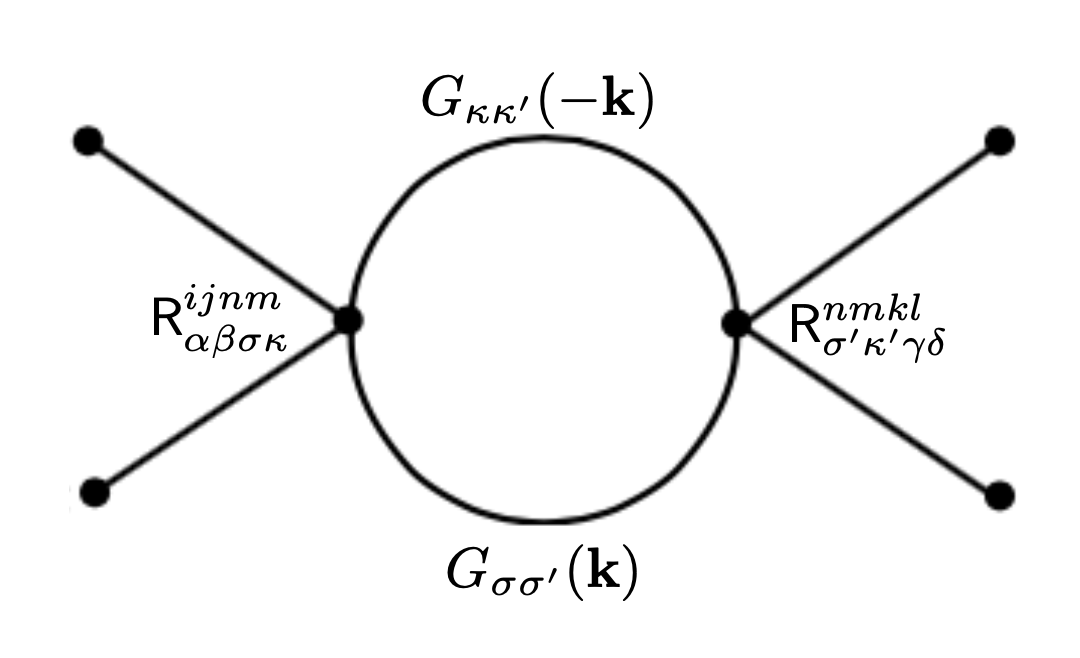
Figure 1: One-loop graphical correction to the symmetrized quartic coupling tensor, $\hat{R}^{ijkl}_{\alpha\beta,\gamma\delta}$.

As usual, because the vertex is independent of momentum, a singular momentum-dependent correction to the inverse propagator only appears at two loops, i.e., the exponent $\eta=0$ within the one-loop calculation on which we focus on here. Henceforth the ratio $\kappa/g$ is not flowing to this order.

At vanishing vertex momentum, the loop integral is rotationally invariant and thus can be easily computed over the spherical momentum shell. We first perform angular average using identities for $\langle\hat{k}_{\alpha}\hat{k}_{\beta}\rangle=\frac{1}{D}\delta_{\alpha\beta}$ and $\langle\hat{k}_{\alpha}\hat{k}_{\beta}\hat{k}_{\gamma}\hat{k}_{\delta}\rangle=\frac{1}{D(D+2)}\left(\delta_{\alpha\beta}\delta_{\gamma\delta}+\delta_{\alpha\gamma}\delta_{\beta\delta}+\delta_{\alpha\delta}\delta_{\gamma\beta}\right)$, which give:

$$\langle P^{L}_{\alpha\beta}P^{L}_{\gamma\delta}\rangle = \frac{1}{D(D+2)}\left(\delta_{\alpha\beta}\delta_{\gamma\delta}+\delta_{\alpha\gamma}\delta_{\beta\delta}+\delta_{\alpha\delta}\delta_{\gamma\beta}\right),$$ (39)

$$\langle P^{L}_{\alpha\beta}P^{T}_{\gamma\delta}\rangle = \frac{1}{D}\delta_{\alpha\beta}\delta_{\gamma\delta}-\frac{1}{D(D+2)}\left(\delta_{\alpha\beta}\delta_{\gamma\delta}+\delta_{\alpha\gamma}\delta_{\beta\delta}+\delta_{\alpha\delta}\delta_{\gamma\beta}\right),$$ (40)

$$\langle P^{T}_{\alpha\beta}P^{T}_{\gamma\delta}\rangle = \left(1-\frac{2}{D}\right)\delta_{\alpha\beta}\delta_{\gamma\delta}+\frac{1}{D(D+2)}\left(\delta_{\alpha\beta}\delta_{\gamma\delta}+\delta_{\alpha\gamma}\delta_{\beta\delta}+\delta_{\alpha\delta}\delta_{\gamma\beta}\right).$$ (41)

We calculate the remaining integral using momentum shell $\int\frac{d^{D}q}{(2\pi)^{D}}\frac{1}{k^{4}}\to{\int_{\Lambda_{\ell}e^{-d\ell}}^{\Lambda_{\ell}}{d^{D}q\over(2\pi)^{D}}}\frac{1}{k^{4}}=C_{D}\frac{1}{\epsilon}(e^{\epsilon d\ell}-1)\Lambda_{\ell}^{-\epsilon}=C_{D}\Lambda_{\ell}^{D-4}d\ell$, where $d\ell$ is the momentum shell width and $C_{D}=S_{D}/(2\pi)^{D}$, with $S_{D}=2\pi^{D/2}/\Gamma(D/2)$ surface area of a $D$-dimensional ball. Putting the above ingredients together and performing the tensor contractions with Mathematica, we find that the correction to the vertex (38) can be accounted for within the parametrization (35) by the following corrections to the couplings $u,v$

$$\delta u = (A_{1}u^{2}+A_{2}v^{2}+A_{3}uv)C_{D}\Lambda_{\ell}^{D-4}d\ell,$$ (42)

$$\delta v = (B_{1}u^{2}+B_{2}v^{2}+B_{3}uv)C_{D}\Lambda_{\ell}^{D-4}d\ell,$$ (43)

where,

$$A_{1} = -\frac{1}{dD(D+2)}\left[(2d+D^{2}+4D+10)\kappa^{-2}+2((d+2)D-2)g^{-1}\kappa^{-1}+(d(D^{2}-2)+D^{3}+5D^{2}-6)g^{-2}\right],$$ (44)

$$A_{2} = -\frac{8}{dD(D+2)}(g^{-1}-\kappa^{-1})^{2},$$ (45)

$$A_{3} = -\frac{4}{dD(D+2)}\left[(D+6)\kappa^{-2}+4Dg^{-1}\kappa^{-1}+(3D^{2}+D-6)g^{-2}\right],$$ (46)

$$B_{1} = -\frac{1}{dD(D+2)}\left[(d+2D+7)\kappa^{-2}-2(d-D+1)g^{-1}\kappa^{-1}+(d+3D^{2}+2D-5)g^{-2}\right],$$ (47)

$$B_{2} = -\frac{1}{dD(D+2)}\left[(dD^{2}+2(d+2)D+12)\kappa^{-2}+8(D+1)g^{-1}\kappa^{-1}+(dD^{3}+(d+8)D^{2}-2(d-2)D-20)g^{-2}\right],\;\;\;\;\;\;\;\;\;$$ (48)

$$B_{3} = -\frac{2}{dD(D+2)}\left[(d(D+2)+D^{2}+3D+6)\kappa^{-2}-8g^{-1}\kappa^{-1}+(d(D^{2}+D-2)+D^{3}+2D^{2}-D+2)g^{-2}\right].$$ (49)

There are a few simple checks that above result passes. The case of $\kappa=g$ and $u=0$ corresponds to an $O(dD)$ symmetric model. The correction to the $O(dD)$ symmetry breaking quartic interaction $u$ vanishes with $u$, i.e., $a_{2}=0$ for $\kappa=g$, consistent with the existence of the $O(dD)$ symmetric Wilson-Fisher critical point. The resulting correction $\delta v\propto-(dD+8)v^{2}/\kappa^{2}$ is consistent with the $N+8$ factor of an $O(N)$ model (with here $N=dD$). Another check is for $d=1$, in which case the $u$ and $v$ terms in (35) cannot be distinguished from each others, and so they reduce to a single combined coupling constant $u+v$. Consistent with this, we find $\delta(u+v)\propto-(u+v)^{2}$ (see below for a more detailed discussion of this case).

We now examine the RG flows on the critical, $\tau_{R}=0$, $u-v$ surface. As usual for the quartic model, the upper critical dimension is $D=4$, and thus we expand in $\epsilon=4-D$. We define the dimensionless couplings

$$\hat{u}=C_{D}\Lambda_{\ell}^{-\epsilon}\,u/\kappa^{2}\,\quad,\quad\hat{v}=C_{D}\Lambda_{\ell}^{-\epsilon}\,v/\kappa^{2}\,\quad,\quad C_{4}=\frac{1}{8\pi^{2}}.$$ (50)

We also introduce the important parameter

$$s=\kappa/g,$$ (51)

whose domain of variation is $s\in[0,+\infty]$, such as $s=0$ corresponds to the membrane (purely longitudinal model) and to the usual crumpling transition, $s=1$ is the isotropic case, and $s=+\infty$ is the purely transverse model.

To derive the flow equations we calculate $\partial_{\ell}(\hat{u},\hat{v})$ taking into account (i) the rescaling (ii) the above corrections to the interaction vertex. Since there are no corrections to the self energy to this one-loop order, there are no other contributions. This leads to the one-loop RG flow equations

$$\partial_{\ell}\hat{u} = \epsilon\hat{u}+a_{1}\hat{u}^{2}+a_{2}\hat{v}^{2}+a_{3}\hat{u}\hat{v},$$ (52)

$$\partial_{\ell}\hat{v} = \epsilon\hat{v}+b_{1}\hat{u}^{2}+b_{2}\hat{v}^{2}+b_{3}\hat{u}\hat{v},$$

with

$$a_{1}=\frac{-1}{12d}(21+d+(6+4d)s+(69+7d)s^{2})\quad,\quad a_{2}=-\frac{1}{3d}(s-1)^{2}\quad,\quad a_{3}=\frac{-1}{3d}(s(23s+8)+5)$$ (53)

$$b_{1}=\frac{-1}{24d}\left((d+51)s^{2}+2(3-d)s+d+15\right)\quad,\quad b_{2}=\frac{-1}{6d}\left((18d+31)s^{2}+10s+6d+7\right)$$

$$b_{3}=\frac{-1}{6d}\left((9d+47)s^{2}-4s+3d+17\right)$$

and we recall that $s=\kappa/g$, to this one-loop order, does not flow. In the large $d$ limit these equations reduce to

$$\partial_{\ell}\hat{u} = \epsilon\hat{u}-\frac{1}{12}\left(7s^{2}+4s+1\right)\hat{u}^{2}$$ (54)

$$\partial_{\ell}\hat{v} = \epsilon\hat{v}-\frac{1}{24}(s-1)^{2}\hat{u}^{2}-\left(3s^{2}+1\right)\hat{v}^{2}-\frac{1}{2}\left(3s^{2}+1\right)\hat{u}\hat{v}$$

I.2 Analysis of the RG equations

Let us now analyse the RG equations, starting by examining some particular cases.

Crumpling transition. The case $s=0$ corresponds to the limit of $g\rightarrow\infty$, i.e. to a single-valued surface constraint on the tangent vector $\vec{t}_{\alpha}$. In that case the flow equations reduce to that for the crumpling transition of a polymerized membrane:

$$\partial_{\ell}\hat{u} = \epsilon\hat{u}-\frac{d+21}{12d}\hat{u}^{2}-\frac{1}{3d}\hat{v}^{2}-\frac{5}{3d}\hat{u}\hat{v},$$ (55)

$$\partial_{\ell}\hat{v} = \epsilon\hat{v}-\frac{d+15}{24d}\hat{u}^{2}-\frac{6d+7}{6d}\hat{v}^{2}-\frac{3d+17}{6d}\hat{u}\hat{v},$$

Simple algebra shows that these equations are equivalent to those obtained by Paczuski, Kardar and Nelson in PKN , when reexpressed in terms of the $4(v-u/D),4u$ couplings. In the large $d$ limit they reduce to

$$\partial_{\ell}\hat{u} = \epsilon\hat{u}-\frac{1}{12}\hat{u}^{2},$$ (56)

$$\partial_{\ell}\hat{v} = \epsilon\hat{v}-\frac{1}{24}\hat{u}^{2}-\hat{v}^{2}-\frac{1}{2}\hat{u}\hat{v},$$

In that limit these equations have four fixed points (FP):

$$\hat{u} = 0,\;\;\hat{v}=0,\;\;\mbox{Gaussian},$$ (57)

$$\hat{u} = 0,\;\;\hat{v}=\epsilon,\;\;\mbox{O($dD$) critical Heisenberg},$$ (58)

$$\hat{u} = 12\epsilon,\;\,v=-2\epsilon,\;\;\mbox{Crumpling transition},$$ (59)

$$\hat{u} = 12\epsilon,\;\;\hat{v}=-3\epsilon,\;\;\mbox{Marginal}.$$ (60)

The Gaussian FP in unstable for $\epsilon>0$. The Heisenberg FP has one unstable direction. The crumpling transition fixed point is fully attractive. The last fixed point has also one unstable direction and lies at the boundary of the physical stability domain, which requires $2\mu+D\lambda\geq 0$, which here means $\hat{u}+4\hat{v}\geq 0$ (we call it ”Marginal” for that reason). This fixed point structure has a counterpart in the $D=4-\epsilon$ RG for the flat phase AL . As noted in PKN , for $d$ finite, the equations (55) have no attractive fixed point for $d<d_{c}\approx 219$. These equations were recently extended to 2 loops (i.e. order $O(\epsilon^{2})$ and it was found that $d_{c}$ decreases with $\epsilon$ Mouhanna .

General finite $s>0$. At large $d$ the equations (54) have the following fixed points, apart from the Gaussian FP which is fully unstable at $\epsilon>0$

$$\hat{u}=0\quad,\quad\hat{v}=\frac{\epsilon}{1+3s^{2}}$$ (61)

$$\hat{u}=\frac{12\epsilon}{s(7s+4)+1}\quad,\quad\hat{v}=\frac{\epsilon}{3s^{2}+1}-\frac{3\epsilon}{s(7s+4)+1}$$ (62)

$$\hat{u}=\frac{12\epsilon}{s(7s+4)+1}\quad,\quad\hat{v}=-\frac{3\epsilon}{s(7s+4)+1}$$ (63)

The Hessian matrix is triangular. The first FP has eigenvalues $(+1,-1)\epsilon$ along $(u,v)$ directions respectively hence it is unstable along $u$. The second FP has eigenvalues $(-1,-1)\epsilon$ and is the only fully stable one. The third FP has eigenvalues $(-1,1)\epsilon$ and is at the boundary of the physical domain (it has $\hat{u}=-3\hat{v}$). Hence we see that for large $d$ the structure of the FP’s does not qualitatively depend on $s$.

Figure 2: A plot of a critical value of the embedding space dimension $d_{c}(s)$ above which there is a stable critical fixed point to the RG flow to one-loop, as a function of $s=\kappa/g$. This fixed point describes a continuous transition to an ordered phase. For $s=0$ it describes the crumpling transition.

Going back to the full RG equations (52),(53), we find that for $d$ finite and large enough, the structure of the FP’s is qualitatively the same as for $d=+\infty$. We find that for any fixed $s$ there is an embedding dimension $d_{c}(s)$ (plotted in Fig. 2) such that for $d>d_{c}(s)$ there is a fully stable FP, and for $d<d_{c}(s)$ there is not. To determine $d_{c}(s)$ one notes that at this bifurcation two FP’s merge and hence the determinant of the Hessian of the RG equations vanishes. Imposing this condition leads to three non-linear equations for $\hat{u},\hat{v},d$ which are easy to solve numerically. They yield $d_{c}(s)$, and also the position of the two FP $(\hat{u}(s),\hat{v}(s))$ when they merge (and move off to the complex plane). One finds that $d_{c}(s)$ decreases fast with $s$ at small $s$, from its value at $s=0$. One finds for instance that (see also Fig. 2)

$$s=0\quad,\quad d_{c}=d_{c}(0)=218.206\quad,\quad(\hat{u}(s),\hat{v}(s))=(11.1348,-2.35165)\epsilon$$ (64)

$$s=1/4\quad,\quad d_{c}(s)=73.7747\quad,\quad(\hat{u}(s),\hat{v}(s))=(4.40623,-0.755289)\epsilon$$ (65)

$$s=1/2\quad,\quad d_{c}(s)=49.3649\quad,\quad(\hat{u}(s),\hat{v}(s))=(2.21725,-0.322653)\epsilon$$ (66)

$$s=1\quad,\quad d_{c}(s)=42.7846\quad,\quad(\hat{u}(s),\hat{v}(s))=(0.870014,-0.11656)\epsilon$$ (67)

$$s=2\quad,\quad d_{c}(s)=46.1284\quad,\quad(\hat{u}(s),\hat{v}(s))=(0.283511,-0.0397547)\epsilon$$ (68)

$$s=10\quad,\quad d_{c}(s)=56.7704\quad,\quad(\hat{u}(s),\hat{v}(s))=(0.0143203,-0.00222716)\epsilon$$ (69)

For $s=1$ one finds that $d_{c}(s=1)$ admits an analytic expression

$$d_{c}(1)=22+12\sqrt{3}\quad,\quad(\hat{u}(1),\hat{v}(1))=\left(\frac{7+5\sqrt{3}}{18},\frac{1-3\sqrt{3}}{36}\right)\epsilon$$ (70)

Interestingly the same condition of vanishing of the Hessian reveals that there is another special dimension $d_{c}^{-}(s)$ where two fixed points merge, and a stable FP again appears for $d<d_{c}^{-}(s)$. One finds

$$s=0\quad,\quad d^{-}_{c}(s)=1.12657\quad,\quad(\hat{u}^{-}(s),\hat{v}^{-}(s))=(1.48178,-1.13827)\epsilon$$ (71)

$$s=1\quad,\quad d^{-}_{c}(s)=22-12\sqrt{3}=1.21539,~{}~{},~{}~{}(\hat{u}^{-}(s),\hat{v}^{-}(s))=\left(\frac{7-5\sqrt{3}}{18},\frac{1+3\sqrt{3}}{36}\right)\epsilon=(-0.0922363,0.172115)\epsilon$$

This critical dimension is very close to $d=1$ (slightly above), we will not study it in details here (see specific discussion below for $s=1$ and also for $d=1$).

Special case $s=+\infty$. One can study the limit $s=\kappa/g\to+\infty$ or equivalently $\kappa\to+\infty$, in which case the $\vec{t}_{\alpha}$ vector field is purely transverse (i.e. the divergence is constrained to vanish, $\partial_{\alpha}\vec{t}_{\alpha}=0$). To this aim one must rescale the couplings, and define

$$\bar{u}=C_{4}\Lambda_{\ell}^{-\epsilon}\,u/g^{2}=s^{2}\hat{u}\quad,\quad\bar{v}=C_{4}\Lambda_{\ell}^{-\epsilon}\,v/g^{2}=s^{2}\hat{v}$$ (72)

One then obtains in the limit $s\to+\infty$,

$$\partial_{\ell}\bar{u} = \epsilon\bar{u}-\frac{(7d+69)\bar{u}^{2}}{12d}-\frac{23\bar{u}\bar{v}}{3d}-\frac{\bar{v}^{2}}{3d}$$ (73)

$$\partial_{\ell}\bar{v} = \epsilon\bar{v}-\frac{(d+51)\bar{u}^{2}}{24d}-\frac{(9d+47)\bar{u}\bar{v}}{6d}-\left(\frac{31}{6d}+3\right)\bar{v}^{2}$$ (74)

At large $d$ the above fixed points become

$$\bar{u}=0\quad,\quad\bar{v}=\frac{\epsilon}{3}$$ (75)

$$\bar{u}=\frac{12\epsilon}{7}\quad,\quad\bar{v}=-\frac{2}{21}\epsilon$$ (76)

$$\bar{u}=\frac{12\epsilon}{7}\quad,\quad\bar{v}=-\frac{3\epsilon}{7}$$ (77)

We know from the discussion above, valid for any $s$, that only the second one is fully stable. For arbitrary $d$, a stable FP exists only for $d>d_{c}(s=+\infty)$ with

$$s=+\infty\quad,\quad d_{c}(s)=61.3112\quad,\quad(\hat{u}(s),\hat{v}(s))=(1.52165,-0.244306)\epsilon$$ (78)

and the second special dimension is $d_{c}^{-}(+\infty)=1.04247$, with $(\hat{u}^{-}(+\infty),\hat{v}^{-}(+\infty))=(-0.411147,0.503785)\epsilon$.

The special case $d=1$. For $d=1$, there is no difference in the action of the initial model between the terms $u,v$. Instead, one obtains an equation for the sum $u+v$. Simply adding the two RG equations in (52) and setting $d=1$ one obtains

$$\partial_{\ell}(\hat{u}+\hat{v})=\epsilon(\hat{u}+\hat{v})-\frac{1}{2}(s(17s+2)+5)(\hat{u}+\hat{v})^{2}$$ (79)

and then there is always an attractive fixed point at

$$\hat{u}+\hat{v}=\frac{2\epsilon}{s(17s+2)+5}$$ (80)

In the transverse only limit $\kappa\to+\infty$, i.e. $s\to+\infty$ in terms of the couplings $\bar{u},\bar{v}$ defined above in (72) we obtain

$$\partial_{\ell}(\bar{u}+\bar{v})=\epsilon(\bar{u}+\bar{v})-\frac{17}{2}(\bar{u}+\bar{v})^{2}$$ (81)

One can check that we obtain the same RG equation as in FreyIsotropicDipolar (see (4.15) there taking $\ell\to+\infty$, with the identification that $u(\ell)$ there equals $6(\bar{u}+\bar{v})$ here, as obtained comparing their action (2.1) with ours - which leads to $u_{0}\equiv 6(u+v)$). In that work they study a Heisenberg model with isotropic dipolar interactions, which corresponds to a $q$-dependent bare $\kappa(q)=g+c/q^{2}$. Its non analytic structure forbids graphical corrections to the amplitude $c$. Here we find that it coincides (beyond some crossover scale) with the limit $\kappa=+\infty$ of our RG equations, which is reasonable to expect.

The special case $s=1$. In that case the propagator is isotropic $\kappa=g$. Our RG equations then become

$$\partial_{\ell}\hat{u}=\epsilon\hat{u}-\frac{\hat{u}}{d}\left((d+8)\hat{u}+12\hat{v}\right)$$ (82)

$$\partial_{\ell}\hat{v}=\epsilon\hat{v}-\frac{1}{d}(\hat{u}+2\hat{v})(2(d+2)\hat{v}+3\hat{u})$$ (83)

For $d\to+\infty$ the stable fixed point is $\hat{u}=\epsilon$ and $\hat{v}=0$.

One can check that these equations are equivalent to those obtained in VicariNM2001 (denoting $u^{\prime}$ and $v^{\prime}$ their couplings, one has $v^{\prime}=6\hat{u}/d$ and $u^{\prime}=6(\hat{u}+\hat{v})/d$). In that paper the standard $O(n)\times O(m)$ model (with $\kappa=g$) is studied to three loops (order $O(\epsilon^{3})$). To make contact with our model for $s=1$ we set $m=D=4$ in their equations. Our model for $s=1$ thus corresponds to $O(n=d)\times O(m=D)$, but where the number of components $m$ is tied to the space dimension $D$. The isotropic fixed point that we obtain here for $s=1$ corresponds to what they call the chiral fixed point. They have a similar structure of FP’s as we discussed above. They also have the Heisenberg $O(mn)$ fixed point, together with an ”anti-chiral FP” which can be compared to our FP that we called marginal. They also note that there are two special values of $n=n^{\pm}(m)$ such that their chiral FP exists and is stable only for $n>n_{+}$ and $n<n_{-}$. This maps onto the special dimensions $d_{c}(1)$, $d_{c}^{-}(1)$ calculated above. To one-loop order, their result reads

$$n^{\pm}(m)=5m+2\pm 2\sqrt{6(m-1)(m+2)}$$ (84)

and setting $n=d$ and $m=D=4$ we recover our results above (70) and (71) for $s=1$. They also compute the correction to $n^{\pm}(m)$ to the next order in $\epsilon$. Within their model this correction reads

$$\epsilon\left(-5m-2\mp\frac{1}{2\sqrt{6(m-1)(m+2)}}(25m^{2}+22m-32)\right)=-(22+\frac{38}{\sqrt{3}})\epsilon\approx-43.9393\epsilon$$ (85)

where we evaluated only the $+$ branch and set $m=4$, so that $n^{+}(4)=42.7846-43.9393\epsilon$. We will refrain from using that result for our model, since in our model $D$ and $m$ are constrained to be equal. Still it is quite analogous to the result obtained to two loops for the crumpling transition in Mouhanna . Finally note that there is an additional critical value of $n$ identified in VicariNM2001 such that for $n<n_{H}(m)=\frac{1}{m}(4-2\epsilon)$ the Heisenberg FP becomes the stable one. Finally, the authors of VicariNM2001 also compute the $\eta$ exponent. From their result we can infer, setting $m=4$

$$\eta=\frac{4d+2}{72}(u^{\prime})^{2}+3(d-1)v^{\prime}(\frac{v^{\prime}}{48}-\frac{u^{\prime}}{36})+h.o.t$$ (86)

To leading order at large $d$ the stable fixed point is at $u^{\prime}=v^{\prime}=6\epsilon/d$ and one finds

$$\eta=\frac{5}{4d}\epsilon^{2}+O(1/d^{2})$$ (87)

which we will compare with our results below. Finally, Ref. VicariNM2001 also computes the exponent $\nu$, which we give here for completeness. In our notations

$$\frac{1}{\nu}=2-\frac{4d+2}{6}u^{\prime}+\frac{d-1}{2}v^{\prime}+h.o.t=2-\frac{d+5}{d}\epsilon+O(\epsilon^{2})$$ (88)

II II. SCSA analysis and large $d$ expansion

In this section we give some of the details of the SCSA calculation, as well as of the large-$d$ expansion. Some more technical details will be given in following sections. The method was pioneered for the $O(N)$ model by Bray in Bray . For membranes it was introduced in LRprl to describe the flat phase and the crumpling transition. We will use similar methods and notations as in Refs. LRReview and OurBuckling to which we refer for more details on the method (see in particular the Appendices and Supp. Mat there).

II.1 Starting model: bare propagator and bare vertex

We will consider again the model at the critical point $\tau_{R}=0$. Since in the SCSA the (dressed) quartic vertex acquires a momentum dependence, we extend the notations and write the bare effective Hamiltonian as

$$H[\vec{r}]=\frac{1}{2}\int_{{\bf k}}\left(\kappa P^{L}_{\alpha\beta}({\bf k})+gP^{T}_{\alpha\beta}({\bf k})\right)k^{2}t_{\alpha}({\bf k})t_{\beta}(-{\bf k})+{1\over{4d}}\int_{{\bf k}_{1},{\bf k}_{2},{\bf k}_{3}}R_{\alpha\beta,\gamma\delta}(\hbox{\bf q})~{}{\vec{t}}_{\alpha}({\bf k}_{1})\cdot{\vec{t}}_{\beta}({\bf k}_{2})~{}{\vec{t}}_{\gamma}({\bf k}_{3})\cdot{\vec{t}}_{\delta}({\bf k}_{4})$$ (89)

with $\hbox{\bf q}={\bf k}_{1}+{\bf k}_{2}$ and ${\bf k}_{1}+{\bf k}_{2}+{\bf k}_{3}+{\bf k}_{4}={\bf 0}$, and we use $\int_{{\bf k}}$ to denote $\int d^{D}k/(2\pi)^{D}$. As before the bare tangent correlator reads

$$\langle t^{i}_{\alpha}({\bf k})t^{j}_{\beta}({\bf k})\rangle_{0}=\delta_{ij}G_{\alpha\beta}({\bf k})(2\pi)^{d}\delta^{d}({\bf k}+{\bf k}^{\prime})$$ (90)

$$G^{-1}_{\alpha\beta}({\bf k})=\left(\kappa P^{L}_{\alpha\beta}({\bf k})+gP^{T}_{\alpha\beta}({\bf k})\right)k^{2}\quad,\quad G_{\alpha\beta}({\bf k})=\frac{P_{\alpha\beta}^{L}({\bf k})}{\kappa k^{2}}+\frac{P_{\alpha\beta}^{T}({\bf k})}{gk^{2}}$$ (91)

We choose the bare quartic tensorial interaction to be local, as in the main text, and of the form:

$$R_{\alpha\beta,\gamma\delta}=\frac{\mu_{0}}{2}(\delta_{\alpha\gamma}\delta_{\beta\delta}+\delta_{\alpha\delta}\delta_{\beta\gamma})+\frac{\lambda_{0}}{2}\delta_{\alpha\beta}\delta_{\gamma\delta}.\quad,\quad\mu_{0}=u\quad,\quad\lambda_{0}=2v$$ (92)

where we use the natural notations in the context of membranes.

II.2 SCSA equations: dressed propagator and dressed vertex

The dressed tangent correlator is denoted as

$$\langle t^{i}_{\alpha}({\bf k})t^{j}_{\beta}({\bf k})\rangle=\delta_{ij}{\cal G}_{\alpha\beta}({\bf k})(2\pi)^{d}\delta^{d}({\bf k}+{\bf k}^{\prime})\quad,\quad{\cal G}^{-1}_{\alpha\beta}({\bf k})=G^{-1}_{\alpha\beta}({\bf k})+\sigma_{\alpha\beta}({\bf k})$$ (93)

where $\sigma_{\alpha\beta}({\bf k})$ is the self-energy. The SCSA gives two self-consistent Dyson type equations for the self-energy and the dressed vertex, which allow to determine the dressed propagator ${\cal G}_{\alpha\beta}({\bf k})$. The infrared behavior of the resulting dressed propagator (e.g. the exponent $\eta$, see below) is by construction exact to first order in the large $d$ expansion, i.e. to order $O(1/d)$ in any $D$ dimension. Similarly the dressed vertex is exact as $d\to\infty$. The SCSA equations ”improve” on the large-$d$ expansion by making it self-consistent through the use of dressed propagators and vertices. It amounts to a resumation of a $1/d$ expansion. It thereby provides predictions for any $D,d$. Since it accounts for the physics of screening of the interaction by fluctuations, it is known to give accurate results for membranes in physical dimensions $d=3$ LRReview .

The first SCSA ”self-energy” equation takes the form

$$\sigma_{\alpha\gamma}({\bf k})={2\over d}\int_{q}\tilde{R}_{\alpha\beta,\gamma\delta}(\hbox{\bf q}){\cal G}_{\beta\delta}({\bf k}-\hbox{\bf q})$$ (94)

where everywhere repeated indices are summed over. Note that in principle it should be symmetrized in $\alpha,\gamma$, however the only two-index tensors which appear here are symmetric. The complete Dyson equation for the self-energy contains an additional (UV divergent) $k$-independent ”tadpole” diagram contribution. The integral in (94) takes also some value at $k=0$. Both contributions have been subtracted by tuning the bare ”mass” term (reduced temperature) $\tau$ to its critical value (so that $\tau_{R}=0$). This is the standard procedure when dealing with a critical theory, where a parameter (distance to crumpling transition parameters) must be tuned. Henceforth, the integral in the r.h.s. of (94) is to be understood with its value at $k=0$ substracted.

In (94) $\tilde{R}_{\alpha\beta,\gamma\delta}(\hbox{\bf q})$ is the (momentum dependent) dressed quartic vertex. It is a four index tensor which is symmetric in $\alpha\leftrightarrow\beta$, in $\gamma\leftrightarrow\delta$ and under the exchange $(\alpha,\beta)\leftrightarrow(\gamma,\delta)$. It is determined by the second SCSA equation, which reads

$$\tilde{R}_{\alpha\beta,\gamma\delta}(\hbox{\bf q}) = R_{\alpha\beta,\gamma\delta}(\hbox{\bf q})-R_{\alpha\beta,\alpha^{\prime}\beta^{\prime}}(\hbox{\bf q})\Pi_{\alpha^{\prime}\beta^{\prime},\gamma^{\prime}\delta^{\prime}}(\hbox{\bf q})\tilde{R}_{\gamma^{\prime}\delta^{\prime},\gamma\delta}(\hbox{\bf q})$$ (95)

where $\Pi_{\alpha\beta,\gamma\delta}(\hbox{\bf q})$ is the four index vacuum polarization tensor, which is also a symmetric tensor

$$\Pi_{\alpha\beta,\gamma\delta}(\hbox{\bf q})={\rm sym}_{\alpha\beta}{\rm sym}_{\delta\gamma}\int_{p}{\cal G}_{\alpha\gamma}({\bf p}){\cal G}_{\beta\delta}(\hbox{\bf q}-{\bf p})$$ (96)

where ${\rm sym}_{\alpha\beta}A_{\alpha\beta}=\frac{1}{2}(A_{\alpha\beta}+A_{\beta\alpha})$.

To solve these equations we first parameterize the momentum-dependent tensors $\Pi$ and $\tilde{R}$ in an appropriate basis of projectors. We now recall how this is done (see ALGolubovic for the original construction of these tensors, and LRReview and OurBuckling for applications within the SCSA).

II.3 Projectors and tensor multiplication, inversion of the second SCSA equation

Here we consider four index tensors, such as $R_{\alpha\beta,\gamma\delta}({\bf q})$ and $\Pi_{\alpha\beta,\gamma\delta}({\bf q})$ introduced above, which are symmetric in $\alpha\leftrightarrow\beta$, in $\gamma\leftrightarrow\delta$ and in $(\alpha,\beta)\leftrightarrow(\gamma,\delta)$. The product of such tensors is defined as $(T\cdot T^{\prime})_{\alpha\beta,\gamma\delta}=T_{\alpha\beta,\gamma^{\prime}\delta^{\prime}}T^{\prime}_{\gamma^{\prime}\delta^{\prime},\gamma\delta}$, the identity being $I_{\alpha\beta,\gamma\delta}={1\over 2}(\delta_{\alpha\gamma}\delta_{\beta\delta}+\delta_{\alpha\delta}\delta_{\beta\gamma})$. We recall the definition LRReview of the five ”projectors” $W_{i}$, $i=1,\ldots,5$, which span the space of such four index tensors

$$(W_{3})_{\alpha\beta,\gamma\delta}({\bf q})={1\over{D-1}}P^{T}_{\alpha\beta}P^{T}_{\gamma\delta}\;,\;\;\;(W_{5})_{\alpha\beta,\gamma\delta}(\hbox{\bf q})=P^{L}_{\alpha\beta}P^{L}_{\gamma\delta}\;,$$ (97)

$$(W_{4})_{\alpha\beta,\gamma\delta}(\hbox{\bf q})=(W_{4a})_{\alpha\beta,\gamma\delta}(\hbox{\bf q})+(W_{4b})_{\alpha\beta,\gamma\delta}(\hbox{\bf q})\;,$$ (98)

$$(W_{4a})_{\alpha\beta,\gamma\delta}(\hbox{\bf q})={1\over{\sqrt{D-1}}}P^{T}_{\alpha\beta}P^{L}_{\gamma\delta}\;,\quad(W_{4b})_{\alpha\beta,\gamma\delta}(\hbox{\bf q})={1\over{\sqrt{D-1}}}P^{L}_{\alpha\beta}P^{T}_{\gamma\delta}\;,$$ (99)

$$(W_{2})_{\alpha\beta,\gamma\delta}(\hbox{\bf q})={1\over 2}(P^{T}_{\alpha\gamma}P^{L}_{\beta\delta}+P^{T}_{\alpha\delta}P^{L}_{\beta\gamma}+P^{L}_{\alpha\gamma}P^{T}_{\beta\delta}+P^{L}_{\alpha\delta}P^{T}_{\beta\gamma})\;,$$ (100)

$$W_{1}(\hbox{\bf q})={1\over 2}(\delta_{\alpha\gamma}\delta_{\beta\delta}+\delta_{\alpha\delta}\delta_{\beta\gamma})-W_{3}(\hbox{\bf q})-W_{5}(\hbox{\bf q})-W_{2}(\hbox{\bf q})\;,$$ (101)

$$W_{1}(\hbox{\bf q})+W_{3}(\hbox{\bf q})={1\over 2}(P^{T}_{\alpha\gamma}(\hbox{\bf q})P^{T}_{\beta\delta}(\hbox{\bf q})+P^{T}_{\alpha\delta}(\hbox{\bf q})P^{T}_{\beta\gamma}(\hbox{\bf q}))$$ (102)

where $P^{T}_{\alpha\beta}=\delta_{\alpha\beta}-q_{\alpha}q_{\beta}/q^{2}$ and $P^{L}_{\alpha\beta}=q_{\alpha}q_{\beta}/q^{2}$ are the standard transverse and longitudinal projection operators associated to q. The first two projectors $W_{1},W_{2}$ are mutually orthogonal and orthogonal to the other three. Note that while $R$, being symmetric, can be expressed in terms of the symmetric tensors $W_{i}$, $i=1,..5$, we will need at some intermediate stages of the calculations some products (such as $\Pi*R$ see below), which are not symmetric. Hence we introduced $W_{4}^{a}$ and $W_{4}^{b}$, which together with $W_{i}$, $i=1,2,3$ and $W_{5}$ make the representation complete under tensor multiplication. The rules for the tensor multiplication $T^{\prime\prime}=T^{\prime}*T$ of the tensors $T=\sum_{i=1}^{3}w_{i}W_{i}+w_{4a}W_{4a}+w_{4b}W_{4b}+w_{5}W_{5}$ and $T^{\prime}=\sum_{i=1}^{3}w^{\prime}_{i}W_{i}+w^{\prime}_{4a}W_{4a}+w^{\prime}_{4b}W_{4b}+w^{\prime}_{5}W_{5}$ are

$$w_{1}^{\prime\prime}=w^{\prime}_{1}w_{1}\;,\;\;\;w_{2}^{\prime\prime}=w^{\prime}_{2}w_{2}\;,\;\;\;\begin{pmatrix}w_{3}^{\prime\prime}&w_{4a}^{\prime\prime}\\ w_{4b}^{\prime\prime}&w_{5}^{\prime\prime}\end{pmatrix}=\begin{pmatrix}w^{\prime}_{3}&w_{4a}^{\prime}\\ w_{4b}^{\prime}&w^{\prime}_{5}\end{pmatrix}\begin{pmatrix}w_{3}&w_{4a}\\ w_{4b}&w_{5}\end{pmatrix}\;,$$ (103)

with $T^{\prime\prime}=\sum_{i=1}^{3}w^{\prime\prime}_{i}W_{i}+w^{\prime\prime}_{4a}W_{4a}+w^{\prime\prime}_{4b}W_{4b}+w^{\prime\prime}_{5}W_{5}$.

Then we define the decomposition of our tensors of interest on this basis (suppressing the indices here)

$$\tilde{R}(\hbox{\bf q})=\sum_{i=1}^{5}\tilde{w}_{i}(\hbox{\bf q})W_{i}(\hbox{\bf q})\;,\quad,\quad\Pi(\hbox{\bf q})=\sum_{i=1}^{5}\pi_{i}(\hbox{\bf q})W_{i}(\hbox{\bf q})\;,$$ (104)

To perform the calculations we need the inversion formula, which allows us to obtain the coefficients (correcting the obvious misprint in (C19) of LRReview )

$$\pi_{1}(\hbox{\bf q}) = \frac{2}{(D-2)(D+1)}(W_{1})_{\alpha\beta,\gamma\delta}\Pi_{\alpha\beta,\gamma\delta}(\hbox{\bf q})$$ (105)

$$\pi_{2}(\hbox{\bf q}) = \frac{1}{D-1}(W_{2})_{\alpha\beta,\gamma\delta}\Pi_{\alpha\beta,\gamma\delta}(\hbox{\bf q})$$ (106)

$$(D-1)\pi_{3}(\hbox{\bf q}) = P^{T}_{\alpha\beta}(\hbox{\bf q})\Pi_{\alpha\beta,\gamma\delta}(\hbox{\bf q})P^{T}_{\gamma\delta}(\hbox{\bf q})\;,$$ (107)

$$\pi_{5}(\hbox{\bf q}) = P^{L}_{\alpha\beta}(\hbox{\bf q})\Pi_{\alpha\beta,\gamma\delta}(\hbox{\bf q})P^{L}_{\gamma\delta}(\hbox{\bf q})\;,$$ (108)

$$\sqrt{D-1}\pi_{4}(\hbox{\bf q}) = P^{L}_{\alpha\beta}(\hbox{\bf q})\Pi_{\alpha\beta,\gamma\delta}(\hbox{\bf q})P^{T}_{\gamma\delta}(\hbox{\bf q})=P^{T}_{\alpha\beta}(\hbox{\bf q})\Pi_{\alpha\beta,\gamma\delta}(\hbox{\bf q})P^{L}_{\gamma\delta}(\hbox{\bf q})\;.$$ (109)

Using (101) the formula for $\pi_{1}(\hbox{\bf q})$ reduces to

$$\pi_{1}(\hbox{\bf q}) = \frac{2}{(D-2)(D+1)}\left[{1\over 2}(\delta_{\alpha\gamma}\delta_{\beta\delta}+\delta_{\alpha\delta}\delta_{\beta\gamma})\Pi_{\alpha\beta,\gamma\delta}(\hbox{\bf q})-\pi_{3}(\hbox{\bf q})-\pi_{5}(\hbox{\bf q})-(D-1)\pi_{2}(\hbox{\bf q})\right]$$ (110)

The bare vertex (92), which is local and q independent, can also be written in this general basis, as

$$R=\sum_{i=1}^{5}w_{i}W_{i}(\hbox{\bf q}),\;\;w_{1}=w_{2}=\mu_{0},\;\;w_{3}=\frac{1}{2}(D-1)\lambda_{0}+\mu_{0},\;\;w_{4}=\frac{1}{2}\sqrt{D-1}\lambda_{0},\;\;w_{5}=\frac{1}{2}\lambda_{0}+\mu_{0}\;.$$ (111)

Note that the q dependence cancels and that the two eigenvalues of the matrix formed by the $w_{i}$, $i=3,4,5$, are then $\mu_{0}$, and $\mu_{0}+\frac{1}{2}D\lambda_{0}$.

We can now formally solve the second SCSA equation (95) and find the renormalized couplings $\tilde{w}_{i}(\hbox{\bf q})$ as functions of the $\pi_{i}(\hbox{\bf q})$ as

$$\tilde{w}_{1}(\hbox{\bf q})={w_{1}\over{1+w_{1}\pi_{1}(\hbox{\bf q})}}\;,\;\;\;\tilde{w}_{2}(\hbox{\bf q})={w_{2}\over{1+w_{2}\pi_{2}(\hbox{\bf q})}}\;,$$ (112)

$$\begin{pmatrix}\tilde{w}_{3}(\hbox{\bf q})&\tilde{w}_{4}(\hbox{\bf q})\\ \tilde{w}_{4}(\hbox{\bf q})&\tilde{w}_{5}(\hbox{\bf q})\end{pmatrix}=\begin{pmatrix}w_{3}&w_{4}\\ w_{4}&w_{5}\end{pmatrix}\left(\begin{pmatrix}1&0\\ 0&1\end{pmatrix}+\begin{pmatrix}\pi_{3}(\hbox{\bf q})&\pi_{4}(\hbox{\bf q})\\ \pi_{4}(\hbox{\bf q})&\pi_{5}(\hbox{\bf q})\end{pmatrix}\begin{pmatrix}w_{3}&w_{4}\\ w_{4}&w_{5}\end{pmatrix}\right)^{-1}\;\;.$$ (113)

These can be substituted into (25) to express the self-energy as

$$\sigma_{\alpha\gamma}({\bf k})={2\over d}\sum_{i=1}^{5}\int_{q}\tilde{w}_{i}(\hbox{\bf q})(W_{i})_{\alpha\beta,\gamma\delta}(\hbox{\bf q}){\cal G}_{\beta\delta}({\bf k}-\hbox{\bf q})$$ (114)

II.4 Ansatz for the propagator at the critical point

We now look for a solution of the SCSA equations which describes the critical manifold, i.e., for a propagator which behaves as a power law at small momentum. A priori one could choose

$${\cal G}^{-1}_{\alpha\beta}({\bf k})\simeq Z_{\kappa}k^{2-\eta}P^{L}_{\alpha\beta}({\bf k})+Z_{g}k^{2-\eta_{g}}P^{T}_{\alpha\beta}({\bf k})\quad,\quad{\cal G}_{\alpha\beta}({\bf k})\simeq\frac{P_{\alpha\beta}^{L}({\bf k})}{Z_{\kappa}k^{2-\eta}}+\frac{P_{\alpha\beta}^{T}({\bf k})}{Z_{g}k^{2-\eta_{g}}}$$ (115)

i.e. two different exponents for the transverse and longitudinal components. However we will restrict our search to the case $\eta_{g}=\eta$, but take into account that there are a priori two distinct amplitudes $Z_{\kappa}$ and $Z_{g}$ for each component. While in SCSA each is non-universal, their ratio may be universal and in this section we will call $s$ their ratio

$$s=\frac{Z_{\kappa}}{Z_{g}}$$ (116)

since it corresponds to a ”dressed” (or renormalized) version of $\kappa/g$. Anticipating that $\eta>0$ we see that at small $k$ we can neglect the bare inverse propagator compared to the dressed one, hence our ansatz for the self-energy is given by

$$\sigma_{\alpha\beta}({\bf k})\simeq k^{2-\eta}\left(Z_{\kappa}P^{L}_{\alpha\beta}({\bf k})+Z_{g}P^{T}_{\alpha\beta}({\bf k})\right)$$ (117)

II.5 Dressed quartic couplings

We start with the calculation of the ”vacuum polarization bubble” $\pi_{(}\hbox{\bf q})$, presenting here only the results and leaving the quite technical derivation to Section III below. The key result is that at small $q$ $\pi_{i}(\hbox{\bf q})$ diverge as (under the condition that $4-D-2\eta>0$)

$$\pi_{i}(\hbox{\bf q})\simeq Z_{\kappa}^{-2}a_{i}(\eta,D,s)q^{-(4-D-2\eta)}\;.$$ (118)

For the amplitudes $a_{i}=a_{i}(\eta,D)$ we find

$$a_{1}=2A\left(\frac{2(\eta-2)^{2}s^{2}(D+\eta-1)}{D+\eta-2}-\frac{2(\eta-2)(2\eta-5)s(s-1)(D+\eta-1)}{(D+1)(D+\eta-2)}+(s-1)^{2}\right)$$ (119)

$$a_{2}=\frac{2A(\eta-2)\left(s\left(D^{2}+D(3\eta-7)+2(\eta-2)^{2}\right)-\left(s^{2}(D(D+\eta-3)-2\eta+3)\right)-1\right)}{D+\eta-2}$$

$$a_{3}=A\left(\frac{4(\eta-2)^{2}s^{2}(D+\eta-1)}{D+\eta-2}+\frac{4(\eta-2)s(s-1)(D+\eta-1)}{D+\eta-2}+D(s-1)^{2}+(s-1)^{2}\right)$$

$$a_{4}=A\sqrt{D-1}(s-1)^{2}(D+2\eta-3)$$

$$a_{5}=\frac{A}{D+\eta-2}\bigg{(}D^{2}(\eta-2)(s-5)(s-1)+D^{3}(s-1)^{2}$$

$$-D\left(-8(\eta-4)\eta+s^{2}+4(\eta-4)\eta s+14s-31\right)+(\eta-2)\left(4\eta^{2}+4\eta(s-4)-s(s+2)+11\right)\bigg{)}$$

where $A$ is defined by (using the same notations as in LRReview )

$$A=\frac{\Pi(\eta,D)}{D^{2}-1}\quad,\quad\Pi(\eta,D)=(D^{2}-1){{\Gamma}(2-\eta-\frac{D}{2}){\Gamma}(\frac{D}{2}+\frac{\eta}{2})^{2}\over 4{(4\pi)^{D/2}}{\Gamma}(2-\frac{\eta}{2})^{2}{\Gamma}(D+\eta)}$$ (120)

A useful check of this result is that for $s=0$ we recover the amplitudes $a_{i}$ obtained for the crumpling transition displayed in Eq. (121) of LRReview .

Now let us look for solutions such that the bare couplings $w_{1}$ and $w_{2}$ are non zero and that the matrix $\begin{pmatrix}w_{3}&w_{4}\\ w_{4}&w_{5}\end{pmatrix}$ is invertible. This is the case for the bare vertex considered in the main text, (111) if we assume $\mu_{0}>0$ and $2\mu_{0}+D\lambda>0$. Note that this excludes some of the (unstable) fixed points discussed in the RG section (see e.g. (57), (61)), that are not of interest to us here.

From (112) in the limit $\hbox{\bf q}\to 0$ we then find

$$\tilde{w}_{1}(\hbox{\bf q})\simeq\frac{1}{\pi_{1}(\hbox{\bf q})}\;,\quad\tilde{w}_{2}(\hbox{\bf q})\simeq\frac{1}{\pi_{2}(\hbox{\bf q})}\quad,\quad\begin{pmatrix}\tilde{w}_{3}(\hbox{\bf q})&\tilde{w}_{4}(\hbox{\bf q})\;,\\ \tilde{w}_{4}(\hbox{\bf q})&\tilde{w}_{5}(\hbox{\bf q})\end{pmatrix}\simeq\begin{pmatrix}\pi_{3}(\hbox{\bf q})&\pi_{4}(\hbox{\bf q})\\ \pi_{4}(\hbox{\bf q})&\pi_{5}(\hbox{\bf q})\end{pmatrix}^{-1}\;.$$ (121)

Hence the dressed couplings are ”soft” (screened), i.e. they vanish at small $q$ as

$$\tilde{w}_{i}(\hbox{\bf q})\simeq Z_{\kappa}^{2}\,c_{i}(\eta,D,s)\,q^{\eta_{u}}\quad,\quad\eta_{u}=4-D-2\eta$$ (122)

where the $c_{i}=c_{i}(\eta,D,s)$ are obtained from the $a_{i}=a_{i}(\eta,D,s)$ given in (119) as

$$c_{1}=\frac{1}{a_{1}}\quad,\quad c_{2}=\frac{1}{a_{2}}\quad,\quad\begin{pmatrix}c_{3}&c_{4}\\ c_{4}&c_{5}\end{pmatrix}\simeq\begin{pmatrix}a_{3}&a_{4}\\ a_{4}&a_{5}\end{pmatrix}^{-1}$$ (123)

II.6 Self-energy

We can now insert this result for $\tilde{w}_{i}(\hbox{\bf q})$ into the first SCSA equation for the self-energy (114), obtaining

$$\sigma_{\alpha\gamma}({\bf k})={2\over d}\sum_{i=1}^{5}\int_{q}\tilde{w}_{i}(\hbox{\bf q})(W_{i})_{\alpha\beta,\gamma\delta}(\hbox{\bf q}){\cal G}_{\beta\delta}({\bf k}-\hbox{\bf q})\simeq Z_{\kappa}^{2}\sum_{i=1}^{5}c_{i}(\eta,D,s)\sigma^{i}_{\alpha\gamma}({\bf k})$$ (124)

where the $\sigma^{i}_{\alpha\gamma}({\bf k})$ are the following integrals

$$\sigma^{i}_{\alpha\gamma}({\bf k})\simeq{2\over d}\int_{q}\,(W_{i})_{\alpha\beta,\gamma\delta}(\hbox{\bf q})\frac{|\hbox{\bf q}|^{4-D-2\eta}}{|{\bf k}-\hbox{\bf q}|^{2-\eta}}\left(\frac{P_{\beta\delta}^{L}({\bf k}-\hbox{\bf q})}{Z_{\kappa}}+\frac{P_{\beta\delta}^{T}({\bf k}-\hbox{\bf q})}{Z_{g}}\right)$$ (125)

These momentum integrals are computed in Section IV. The result can be written as follows

$$\sigma^{i}_{\alpha\gamma}({\bf k})=\frac{2}{d}k^{2-\eta}\frac{1}{Z_{\kappa}}(b_{i}^{(1)}(\eta,D,s)P_{\beta\delta}^{T}({\bf k})+b_{i}(\eta,D,s)P_{\beta\delta}^{L}({\bf k}))$$ (126)

where the amplitudes $b^{1}_{i}=b_{i}^{(1)}(\eta,D,s)$ and $b_{i}=b_{i}(\eta,D,s)$ are given by

$$b_{1}^{1}=-\frac{B(D-2)(D+1)\left(D^{2}((3\eta-4)s-1)+D^{3}s-D(\eta+2s-2)-2(\eta-2)((2(\eta-2)\eta+3)s-\eta)\right)}{2(D-1)(D+\eta-2)}$$

$$b_{2}^{1}=\frac{B\left(D^{2}(-\eta(s+2)+s+4)-D^{3}+D\left(\eta^{2}-3\eta-2(\eta-2)^{2}s+4\right)+2\left((\eta-2)^{3}+(2\eta-3)(\eta-2)s\right)\right)}{D+\eta-2}$$

$$b_{3}^{1}=\frac{B\left(D^{2}(5-3\eta)s+D^{3}(-s)+D(\eta-1)s+D+(\eta-2)(-2\eta+(4(\eta-2)\eta+5)s+1)\right)}{(D-1)(D+\eta-2)}$$

$$b_{4}^{1}=\frac{2B(2\eta-3)(s-1)}{\sqrt{D-1}}$$

$$b_{5}^{1}=B(D(s-2)-2\eta+s+1)$$

as well as

$$b_{1}=-\frac{1}{2}B(D-2)(D+1)(Ds+2\eta s-2)$$ (128)

$$b_{2}=-\frac{B(D-1)\left(D^{2}-s\left(D((\eta-7)\eta+8)+2(\eta-2)^{3}\right)+2\eta-4\right)}{D+\eta-2}$$

$$b_{3}=B(-2s(D+\eta)+D+s+1)$$

$$b_{4}=-2B\sqrt{D-1}(2\eta-3)(s-1)$$

$$b_{5}=\frac{B\left(D^{2}(s-2)-D(2\eta-3)(\eta(s-2)-s+5)+(\eta-2)(2\eta(2\eta+s-8)-s+11)\right)}{D+\eta-2}$$

where we have defined, as in LRReview

$$B=\frac{\Sigma(\eta,D)}{D^{2}-1}\quad,\quad\Sigma(\eta,D)=\frac{\left(D^{2}-1\right)\Gamma(2-\eta)\Gamma\left(\frac{D}{2}+\frac{\eta}{2}\right)\Gamma\left(\eta/2\right)}{4(4\pi)^{D/2}\Gamma\left(2-\frac{{\eta}}{2}\right)\Gamma\left(\frac{D}{2}+\eta\right)\Gamma\left(\frac{D}{2}-\frac{{\eta}}{2}+2\right)}$$ (129)

As a useful check for $s=0$ we recover the amplitudes $b_{i}$ obtained for the crumpling transition in Eq. (124) of LRReview .

II.7 Self-consistency conditions

Now we are ready to derive the final self-consistency conditions. To this end we equate the self-energy obtained by computing the integrals in (124), (125) with our ansatz for the self-energy (117),

$$\sigma_{\alpha\beta}({\bf k})\simeq k^{2-\eta}\left(Z_{\kappa}P^{L}_{\alpha\beta}({\bf k})+Z_{g}P^{T}_{\alpha\beta}({\bf k})\right)\simeq\frac{2}{d}Z_{\kappa}k^{2-\eta}\sum_{i=1}^{5}c_{i}(\eta,D,s)(b_{i}^{(1)}(\eta,D,s)P_{\beta\delta}^{T}({\bf k})+b_{i}(\eta,D,s)P_{\beta\delta}^{L}({\bf k}))$$ (130)

We observe that the non-universal amplitude $Z_{\kappa}$ cancels, giving two self-consistency conditions

$$\frac{d}{2}=F(\eta,D,s)\quad,\quad F(\eta,D,s)=\sum_{i=1}^{5}c_{i}(\eta,D,s)b_{i}(\eta,D,s)$$ (131)

$$\frac{d}{2}=F_{1}(\eta,D,s)\quad,\quad F_{1}(\eta,D,s)=s\sum_{i=1}^{5}c_{i}(\eta,D,s)b^{1}_{i}(\eta,D,s)$$ (132)

where the first equation comes from identifying the longitudinal part and the second the transverse part of the self-energy in (130). Using the relations (123) between the $c_{i}(\eta,D,s)$ and the $a_{i}(\eta,D,s)$ one obtains the explicit expressions for the functions $F_{1}=F_{1}(\eta,D,s)$ and $F=F(\eta,D,s)$ (with the dependence on $\eta,D,s$ suppressed)

$$F_{1}={b_{1}\over a_{1}}+\frac{b_{2}}{a_{2}}+{b_{3}a_{5}-b_{4}a_{4}+b_{5}a_{3}\over{a_{3}a_{5}-a_{4}^{2}}}\quad,\quad F_{1}=s\left({b^{1}_{1}\over a_{1}}+\frac{b^{1}_{2}}{a_{2}}+{b^{1}_{3}a_{5}-b^{1}_{4}a_{4}+b^{1}_{5}a_{3}\over{a_{3}a_{5}-a_{4}^{2}}}\right)$$ (133)

The expressions of the $a_{i}=a_{i}(\eta,D,s)$ and the $b_{i}=b_{i}(\eta,D,s)$ are given in (119), (120) and in (II.6), (129).

A priori the two equations (131) determine the possible fixed point values of the pair $(\eta,s)$ for any given $D<4$. However, as we will show below, and as is confirmed by a numerical search, there appears to be only three possible solutions corresponding to $s=0,1,+\infty$. Let us first discuss each of these special cases. Then, in the next subsection, we give an interpretation of these three solutions as fixed points of an RG flow.

Crumpling transition $s=0$. In the limit $g\to+\infty$, i.e. $s\to 0$ the tangent fields are purely longitudinal and one expects to recover the crumpling transition. Setting $s=0$ in the first equation in (131) gives

$$\frac{d}{2}=\frac{D(D+1)(D+\eta-4)(D+2\eta-4)(2D+2\eta-3)\Gamma(2-\eta)\Gamma\left(2-\frac{\eta}{2}\right)\Gamma\left(\frac{\eta}{2}\right)\Gamma(D+\eta)}{4(\eta-2)(D+\eta-1)(D+2\eta-5)\Gamma\left(-\frac{D}{2}-\eta+2\right)\Gamma\left(\frac{1}{2}(D-\eta+4)\right)\Gamma\left(\frac{D}{2}+\eta\right)\Gamma\left(\frac{D+\eta}{2}\right)}$$ (134)

which coincides with the SCSA equation which determines the exponent $\eta=\eta_{cr}(D,d)$ for the crumpling transition, LRprl , see in LRReview . In $D=2$ it reduces to the root of a cubic equation (with the smallest positive root as the physical solution)

$$\frac{d}{2}=\frac{12(\eta-1)^{2}(2\eta+1)}{(\eta-4)\eta(2\eta-3)}$$ (135)

which leads to the prediction $\eta_{cr}(D=3,d=2)=0.5352..$ for physical membranes LRprl . Let us recall that at large $d$ it gives

$$\eta_{cr}(D,d)\simeq\frac{C(D)}{d}+O(1/d^{2})\quad,\quad C(D)=\frac{(D-4)^{2}(2D-3)\Gamma(D+2)}{2(5-D)(D-1)\Gamma\left(2-\frac{D}{2}\right)\Gamma\left(\frac{D}{2}+2\right)\Gamma\left(\frac{D}{2}\right)^{2}}\;,$$

where $C(D)$ is exact by construction and agrees with the straight $1/d$ expansion PaczuskiCrumplingLarged ; ALGolubovic . Expanding in $D=4-\epsilon$ one obtains

$$\eta_{cr}(D,d)\simeq\frac{25}{3d}\epsilon^{3}+O(\epsilon^{4})\quad,\quad$$ (136)

This result, which is $O(\epsilon^{3})$, is consistent with the recent three loop RG calculation in Ref. Mouhanna . Since the SCSA builds on a large $d$ limit, it does not see the disappearance of the critical point at $d=d_{c}\approx 219$, found in the RG to $O(\epsilon)$, leading to a runaway flow, often interpreted as a first order transition. The solution of the SCSA describes instead a second-order critical crumpling transition which survives for any $d$. Interestingly, it was obtained in Ref. Mouhanna that to the next order, $d_{c}=218.20-448.25\epsilon$ decreases quite fast as $D$ is lowered, suggesting that the crumpling critical point may survive to physical dimensions, $D=2$, $d=3$.

It is important to note that strictly for $s=0$ the second SCSA equation in (131) must be dropped, i.e. does not apply. This is despite the fact that the r.h.s. of (130) contains a correction to the transverse part of the self-energy, proportional to $F_{1}(\eta,D,s)/s=\sum_{i=1}^{5}c_{i}(\eta,D,s)b^{1}_{i}(\eta,D,s)$, which, as one can check, remains finite for $s\to 0$. This correction is immaterial for $s=0$, since in that limit the tangent field is purely longitudinal, and hence any term proportional to $\vec{t}_{\alpha}(\hbox{\bf q})P^{T}_{\alpha\beta}(\hbox{\bf q})\cdot\vec{t}_{\beta}(\hbox{\bf q})$ identically vanishes. An analogous remark applies to the limit $s\to+\infty$, which is considered below.

Isotropic critical point, ”tattered” $s=1$. This solution corresponds to $Z_{\kappa}=Z_{g}$, i.e. to an isotropic propagator with $\kappa=g$ in a renormalized sense. It describes a tattered membrane at criticality. For $s=1$ one finds

$$F_{1}(\eta,D,s=1)=F(\eta,D,s=1)$$ (137)

The two equations (131) reduce to a single one,

$$\frac{d}{2}=-\frac{(D+1)(D-\eta+2)(D+2\eta-4)(D+2\eta-2)\Gamma(2-\eta)\Gamma\left(2-\frac{\eta}{2}\right)\Gamma\left(\frac{\eta}{2}\right)\Gamma(D+\eta)}{8(\eta-2)^{2}(D+\eta-1)\Gamma\left(-\frac{D}{2}-\eta+2\right)\Gamma\left(\frac{1}{2}(D-\eta+4)\right)\Gamma\left(\frac{D}{2}+\eta\right)\Gamma\left(\frac{D+\eta}{2}\right)}$$ (138)

which can equivalently be written in a slightly shorter form as

$$\frac{d}{2}=\frac{(D+1)2^{D+\eta-4}(D+2\eta-4)\csc\left(\frac{\pi\eta}{2}\right)\Gamma(2-\eta)\sin\left(\frac{1}{2}\pi(D+2\eta)\right)\Gamma\left(\frac{1}{2}(D+\eta-1)\right)}{\sqrt{\pi}(2-\eta)\Gamma\left(\frac{1}{2}(D-\eta+2)\right)}$$ (139)

We can now look at the large $d$ expansion of $\eta$, by expanding the r.h.s. for small $\eta$, obtaining

$$\eta=\frac{2}{d}C(D)+O(\frac{1}{d^{2}})\quad,\quad C(D)=-\frac{(D-4)(D-2)(D+1)(D+2)\Gamma(D)}{16(D-1)\Gamma\left(2-\frac{D}{2}\right)\Gamma\left(\frac{D}{2}\right)^{2}\Gamma\left(\frac{D+4}{2}\right)}=\frac{2^{D-4}(D-4)(D+1)\sin\left(\frac{\pi D}{2}\right)\Gamma\left(\frac{D-1}{2}\right)}{\pi^{3/2}\Gamma\left(\frac{D}{2}+1\right)}$$ (140)

We find that $C(D)$ vanishes for $D=2$ and $D=4$, and is positive in-between, with a maximum a bit below $D=3$, with

$$C(3)=\frac{8}{3\pi^{2}}\quad,\quad C(D)=\frac{3(D-2)}{4}+O\left((D-2)^{2}\right)\quad,\quad C(D=4-\epsilon)=\frac{5}{8}\epsilon^{2}+O\left(\epsilon^{3}\right)$$ (141)

The vanishing of $\eta$ in $D=2$ to this order is consistent with a lower critical dimension of the tattered membrane critical point equal to $2$. However, the stability of the ordered phase of the tattered membrane remains an open problem that we leave for future studies.

The above results can be compared with the predictions by Bray for the $O(d)$ model at first order in $O(1/d)$. We find

$$C(D)=\frac{D+1}{2}C_{O(d)}(D)\quad,\quad C_{O(d)}(D)=\frac{2(4-D)\Gamma(D-2)}{D\Gamma\left(2-\frac{D}{2}\right)\Gamma\left(\frac{D}{2}-1\right)^{2}\Gamma\left(\frac{D}{2}\right)}$$ (142)

As already discussed in the RG section we expect our isotropic ”tattered membrane” fixed point for $s=1$ to be directly related to the so-called ”chiral” critical fixed point of the model $O(n)\times O(m)$ studied in e.g. VicariNM2001 , provided one identifies $n=d$ and $m=D$ the space dimension. With this correspondence, to leading order in $1/n$ VicariNM2001 , their result for $\eta$ translates into

$$\eta=\frac{2}{d}\frac{D+1}{2}C_{O(d)}(D)+O(\frac{1}{d^{2}})$$ (143)

which agrees with our prediction. They have pushed their analysis to second order in $1/n$. For general $D$ it leads to a complicated expression, which simplifies for $D=3$. Setting $m=D=3$ in their result (Eq. (4.43) there) gives

$$\eta=\frac{16}{3\pi^{2}d}-\frac{608}{27\pi^{4}d^{2}}+O(1/d^{3})$$ (144)

This can be directly compared to the SCSA, which gives a result for general $d$. Expanding this result to the next order in $1/d$ we find for $D=3$

$$\eta=\frac{2}{d}C(3)-\frac{14C(3)^{2}}{3d^{2}}=\frac{16}{3\pi^{2}d}-\frac{896}{27\pi^{4}d^{2}}+O(1/d^{3})$$ (145)

While the leading term agrees, the next order correction in the SCSA is an approximation, but gives a value reasonably close to the exact result at second order in $O(1/d^{2})$.

In $D=3$ and finite $d$, the SCSA gives the equation at the isotropic fixed point, together with their numerical solutions

$$\frac{d}{2}=\frac{8(1-2\eta)\eta\cot\left(\frac{\pi\eta}{2}\right)\cot(\pi\eta)}{(3-\eta)(2-\eta)}$$ (146)

$$\eta_{D=3,d=1}\approx 0.250337\quad,\quad\eta_{D=3,d=2}\approx 0.177214\quad,\quad\eta_{D=3,d=3}\approx 0.136135\quad,\quad\eta_{D=3,d=4}\approx 0.11$$ (147)

In exactly $D=2$ (or as $D\to 2^{+}$) the SCSA naively gives a finite limit for $\eta$ for $d\leq 3$. Indeed the function $F(\eta,D=2^{+},s=1)$ is a non-trivial fonction of $\eta$ decreasing from $3/2$ at $\eta=0$ to $0$ at $\eta=1$. However at $D=2$ this branch is not continuously connected to $\eta=0$ at $d=\infty$, hence it may be a spurious solution.

Finally, around $D=4$ we note that the SCSA gives the same result $\eta\simeq\frac{5}{4d}\epsilon^{2}$ as the straight $1/d$ expansion, consistent with the $O(\epsilon^{2})$ calculation in VicariNM2001 , see Eq. (87).

Transverse critical fixed point, $s=+\infty$. We also find another fixed point for $s=+\infty$ corresponding to $\kappa\to+\infty$. In that case the $\vec{t}_{\alpha}$ vector field is purely transverse. In $D=2$ since $P^{T}_{\alpha,\beta}(\hbox{\bf q})=\hbox{\bf q}^{T}_{\alpha}\hbox{\bf q}^{T}_{\beta}$, where $\hbox{\bf q}^{T}$ is orthogonal to q, there is an exact duality in momentum space, $\hbox{\bf q}\to\hbox{\bf q}^{T}$ which maps this case onto $\vec{t}_{\alpha}$ vector field which are purely longitudinal, i.e. onto the membrane and the crumpling transition. This mapping extends to the low-temperature phase, and thus predicts that this ”transverse” model exhibits an ordered phase in $D=2$, dual of the flat phase of crystalline membranes.

Duality for $D=2$ and arbitrary $s$. Before studying $s=+\infty$ let us comment on this duality within SCSA for general $s$, and that it relates $s\to 1/s$. Indeed, one can check on the explicit formula that the two functions which appear in (131) are related according to

$$F_{1}(\eta,D=2,s)=F(\eta,D=2,1/s)$$ (148)

This is a non-trivial identity, which provides a good check of the calculations. It is a consequence of the above duality $\hbox{\bf q}\leftrightarrow\hbox{\bf q}^{T}$ in momentum space.

Absence of other SCSA solutions One application of this formula is that in $D=2$ it is now simple to exclude solutions of SCSA for finite $s$ apart from $s=1$. Indeed Eqs. (131) and (148) imply that

$$\frac{d}{2}=F_{1}(\eta,D=2,s)=F_{1}(\eta,D=2,1/s)$$ (149)

so one can check whether $F_{1}$ intersects $d/2$ for two different values of $s$. But a plot of $F_{1}$ for fixed $\eta\in[0,1]$ shows that it is a monotonic function of $s$. To further exclude solutions at finite $s\neq 1$ in $D=3$ one can instead plot both $F_{1}(\eta,D,s),F(\eta,D,s)$ for fixed $\eta\in[0,1]$ and check that it has a single intersection at $s=1$.

Let us now return to the SCSA fixed point at $s=+\infty$. Again one of the two equations in (131) drops out, this time only the second equation remain, so $\eta$ is determined by

$$1=\frac{2}{d}F_{1}(\eta,D,+\infty)$$ (150)

The r.h.s. is complicated for general $D$. For $D=2$ one recovers exactly the equation (135) which determines the crumpling exponent, hence $\eta=\eta_{cr}(D=2,d)$.

For $D=3$ it gives

$$\frac{d}{2}=\frac{8\eta(1-2\eta)\left(24\eta^{6}-40\eta^{5}-321\eta^{4}+410\eta^{3}+1119\eta^{2}-1042\eta-990\right)\cot\left(\frac{\pi\eta}{2}\right)\cot(\pi\eta)}{(\eta-5)(\eta-3)(\eta+3)(2\eta+1)(3\eta-5)\left(2\eta^{3}-3\eta^{2}-6\eta+14\right)}$$ (151)

which can be compared with the equation which determines $\eta$ for the crumpling transition in $D=3$, from (134)

$$\frac{d}{2}=\frac{24\eta(1-2\eta)(2\eta+3)\cot\left(\frac{\pi\eta}{2}\right)\cot(\pi\eta)}{(\eta-5)(\eta-3)(2\eta+1)}$$ (152)

and one can see that for general $D>2$ the two fixed points are quite different. This leads to the values

$$\eta_{cr}=0.329074\quad,\quad\eta_{tr}=0.299348\quad,\quad D=3,d=1$$ (153)

$$\eta_{cr}=0.273121\quad,\quad\eta_{tr}=0.233722\quad,\quad D=3,d=2$$ (154)

$$\eta_{cr}=0.23632\quad,\quad\eta_{tr}=0.192301\quad,\quad D=3,d=3$$ (155)

$$\eta_{cr}=0.209223\quad,\quad\eta_{tr}=0.163235\quad,\quad D=3,d=4$$ (156)

hence the $\eta=\eta_{tr}$ exponent of the transverse FP is smaller than the one for crumpling critical point. The large $d$ expansion of the SCSA result gives $\eta=\frac{2}{d}C_{\rm tr}(D)+O(1/d^{2})$ with

$$C_{\rm tr}(D)=\frac{(4-D)(D+1)\left(4D^{8}-22D^{7}+43D^{6}-62D^{5}+228D^{4}-623D^{3}+802D^{2}-464D+96\right)\Gamma(D)}{4(D-1)^{2}(2D-1)(3D-5)(3D-2)\left(D^{2}-3D+3\right)\Gamma\left(2-\frac{D}{2}\right)\Gamma\left(\frac{D}{2}\right)^{2}\Gamma\left(\frac{D+4}{2}\right)}$$ (157)

to be compared with the analogous result for crumpling in (II.7). One finds $C_{\rm tr}(2)=1$ which is the same as for crumpling. For $D=3$ one finds $C_{\rm tr}(3)=176/(35\pi^{2})\approx 0.509501$, significantly smaller than $C(3)=48/(5\pi^{2})\approx 0.972683$ for the crumpling transition.

Finally around $D=4$ the SCSA gives for the transverse FP

$$\eta=\frac{16\epsilon^{2}}{9d}+O(\epsilon^{3})$$ (158)

which coincides with the exact $O(1/d)$ expansion, and is distinct from the $\eta$ exponents for crumpling and for the isotropic critical points.

Lower critical dimension. Finally, we can obtain the lower critical dimension of the transverse fixed point. It is defined by the relation $2-\eta(D_{lc},d)=D_{lc}$. Inserting the relation $\eta=2-D$ inside the equation $F_{1}(\eta,D,+\infty)=d/2$ we obtain that $D=D_{lc}(d)$ is the root of

$$d=\frac{D\left(D^{4}-D^{3}-7D^{2}+5D+8\right)}{2(D-2)(D-1)\left(D^{2}-D-1\right)}$$ (159)

One finds (one must choose the branch continuously related to $D=D_{lc}(+\infty)=2$)

$$D_{lc}(d)=2-\frac{2}{d}-\frac{8}{d^{2}}-\frac{26}{d^{3}}+O(1/d^{4})$$ (160)

$$D_{lc}(40)=1.94462~{},~{}D_{lc}(20)=1.87777~{},~{}D_{lc}(10)=1.75041~{},~{}$$ (161)

$$D_{lc}(4)=1.68255~{},~{}D_{lc}(3)=1.67661~{},~{}D_{lc}(2)=1.67159~{},~{}D_{lc}(1)=1.66732~{},~{}D_{lc}(0)=1.66364$$ (162)

The function $D_{lc}(d)$ varies mostly for $d$ of order $10-20$. Let us recall that for the crumpling transition has a much simpler expression $D_{lc}=2d/(1+d)$.

II.8 RG version of SCSA and flow of $s=\kappa/g$

To understand why there are only three critical fixed points discussed above, we now use SCSA to derive the RG flow of the parameter $s=s(\ell)=\kappa/g$ at scale $k=\Lambda e^{-\ell}$.

As was explained in details in OurBuckling (see section C.3. of the Supp. Mat. there) one can recast the SCSA equations into an RG flow. It can be done so as to recover either (i) only the RG functions to first order in $1/d$, or (ii) within the full self-consistent scheme. We will only consider here the first approach, which is exact to $O(1/d)$.

Refering to OurBuckling for details, one defines within the SCSA the natural dimensionless coupling for the RG as

$$\hat{w}_{i}:=\tilde{w}_{i}(q)Z_{\kappa}^{-2}q^{-\epsilon}$$ (163)

In terms of these couplings we obtain the RG equation for $d=+\infty$, exact for any $\epsilon=4-D$, by taking a derivative $\partial_{\ell}=-q\partial_{q}$ on both sides of (112) and using (118). This gives

$$\partial_{\ell}\hat{w}_{i}=\epsilon\hat{w}_{i}-\epsilon a_{i}(0,D,s)\hat{w}_{i}^{2}\quad,\quad i=1,2$$ (164)

$$\partial_{\ell}\begin{pmatrix}\hat{w}_{3}&\hat{w}_{4}\\ \hat{w}_{4}&\hat{w}_{5}\end{pmatrix}=\epsilon\begin{pmatrix}\hat{w}_{3}&\hat{w}_{4}\\ \hat{w}_{4}&\hat{w}_{5}\end{pmatrix}-\epsilon\begin{pmatrix}\hat{w}_{3}&\hat{w}_{4}\\ \hat{w}_{4}&\hat{w}_{5}\end{pmatrix}\begin{pmatrix}a_{3}(0,D,s)&a_{4}(0,D,s)\\ a_{4}(0,D,s)&a_{5}(0,D,s)\end{pmatrix}\begin{pmatrix}\hat{w}_{3}&\hat{w}_{4}\\ \hat{w}_{4}&\hat{w}_{5}\end{pmatrix}$$ (165)

where the functions $a_{i}(\eta,D,s)$ are those defined in (118) and given in (119), (120). Here, since $\eta=O(1/d)$, they have to be evaluated at $\eta=0$, where they reach finite values. Whenever $s$ can be considered as fixed, the fixed point of these RG equations is $\hat{w}_{i}=\hat{w}_{i}^{*}$ with

$$\hat{w}_{i}^{*}=\frac{1}{a_{i}(0,D,s)}\quad,\quad i=1,2\quad,\quad\begin{pmatrix}\hat{w}^{*}_{3}&\hat{w}^{*}_{4}\\ \hat{w}^{*}_{4}&\hat{w}^{*}_{5}\end{pmatrix}=\begin{pmatrix}a_{3}(0,D,s)&a_{4}(0,D,s)\\ a_{4}(0,D,s)&a_{5}(0,D,s)\end{pmatrix}^{-1}$$ (166)

However, $s$, defined as the renormalized value of $\kappa/g$ has a non-trivial RG flow. To obtain this flow we apply $-k\partial_{k}$ to the equation for the self-energy as explained in OurBuckling . Here it is convenient to define the transverse and longitudinal components of the self-energy, within the SCSA, and write them as

$$\sigma_{T}(k)\simeq Z_{g}k^{2-\eta}=Z_{g}(k)k^{2}$$ (167)

$$\sigma_{L}(k)\simeq Z_{\kappa}k^{2-\eta}=Z_{\kappa}(k)k^{2}$$ (168)

We then define the two ”$\eta$ functions” or anomalous dimensions of $\kappa$ and $g$ respectively as

$$\eta_{g}=-k\partial_{k}\log Z_{g}(k)=-\frac{1}{Z_{g}(k)}k\partial_{k}(\sigma_{T}(k)/k^{2})$$ (169)

$$=-\frac{1}{Z_{g}(k)}k\partial_{k}(\frac{2}{d}Z_{\kappa}(k)\sum_{i=1}^{5}\hat{w}_{i}b_{i}^{1}(\eta,D,s))\simeq\frac{2}{d}s\sum_{i=1}^{5}\hat{w}_{i}\tilde{b}_{i}^{1}(D,s)\quad,\quad\tilde{b}_{i}^{1}(D,s)=\lim_{\eta\to 0}(\eta b_{i}^{1}(\eta,D,s)))$$ (170)

Similarly we define

$$\eta_{\kappa}=-k\partial_{k}\log Z_{\kappa}(k)\simeq\frac{2}{d}\sum_{i=1}^{5}\hat{w}_{i}\tilde{b}_{i}(D,s)\quad,\quad\tilde{b}_{i}(D,s)=\lim_{\eta\to 0}(\eta b_{i}^{1}(\eta,D,s)))$$ (171)

where we substitute the fixed point values for $\hat{w}_{i}$ in (166) for a given $s$, and we work to first order in $O(1/d)$. Using the definitions in (131) it can also be written as

$$\eta_{g}=\frac{2}{d}f_{1}(D,s)\quad,\quad f_{1}(D,s)=\lim_{\eta\to 0}\eta F_{1}(\eta,D,s)$$ (172)

$$\eta_{\kappa}=\frac{2}{d}f(D,s)\quad,\quad f(D,s)=\lim_{\eta\to 0}\eta F(\eta,D,s)$$ (173)

We can now write the flow of $s=\kappa/g$ as

$$\partial_{\ell}s=(\eta_{\kappa}-\eta_{g})\,s=\frac{2}{d}\left[f(D,s)-f_{1}(D,s)\right]\,s$$ (174)

Its expression as a function of general $s,D$ is quite cumbersome, so we focus on the main features.

First we find that $f(D,s=1)=f_{1}(D,s=1)$ for any $D$ in (174) so that for $\kappa=g$, $s$ does not flow, hence it corresponds to a fixed point which describes the critical point for an isotropic tattered membrane. One obtains the explicit expressions in $D=3$, near $D=2$ and near $D=4$

$$\frac{d}{2}(\eta_{\kappa}-\eta_{g})=-\frac{16(s-1)\left(495s^{5}+377s^{4}+238s^{3}+246s^{2}+43s+9\right)}{15\pi^{2}(s+1)^{2}(3s+1)(7s+1)\left(5s^{2}+2s+1\right)}\quad,\quad D=3$$ (175)

$$=-\frac{(D-2)(s-1)\left(3s^{2}-2s+3\right)}{8s(s+1)}+O((D-2)^{2})$$ (176)

$$=-\frac{8(s-1)s\left(49s^{4}+2s^{3}+21s^{2}+8s+4\right)\epsilon^{2}}{3\left(3s^{2}+1\right)\left(7s^{2}+4s+1\right)^{2}}+O(\epsilon^{3})\quad,\quad D=4-\epsilon$$ (177)

One sees that the flow of $s$ vanishes in $D=2$ for any fixed $s>0$ and finite, as in fact both exponents $\eta_{\kappa}$ and $\eta_{g}$ vanish in that limit. However the limits $s\to 0$ and $D\to 2$, as well as $s\to+\infty$ and $D\to 2$ do not commute, as the points $s=0,+\infty$ are special (and dual to each others in $D=2$, as discussed above).

We now extract the behavior of the flow of $s$ around its three fixed points $s=0,1,+\infty$.

(i) Linearizing (174) around $s=1$, one finds, for general $D$, up to $O(1/d^{2})$ terms

$$\eta_{\kappa}-\eta_{g}=\omega_{1}(D,d)(s-1)+O\left((s-1)^{2}\right)$$ (178)

$$\omega_{1}(D,d)=-\frac{2}{d}\frac{(4-D)(D-2)\left(D^{3}-D^{2}+4D-8\right)\Gamma(D)}{16(D-1)^{2}\Gamma\left(2-\frac{D}{2}\right)\Gamma\left(\frac{D}{2}+2\right)\Gamma\left(\frac{D}{2}\right)^{2}}$$ (179)

This defines an eigenvalue exponent $\omega_{1}=\omega_{1}(D,d)$, such that $s-1$ flows as $k^{-\omega_{1}}$ for $k\to 0$. We find that $\omega_{1}(D,d)$ vanishes for $D=2$ as $\omega_{1}(D,d)\simeq-(D-2)/(2d)$, and for $D=4$ as $\omega_{1}(D=4-\epsilon,d)\simeq-7\epsilon^{2}/(9d)$, and is negative in between with $\omega_{1}(D=3,d)=-44/(15d\pi^{2})$. Hence $s$ flows to $1$ at large scale, and the isotropic tattered membrane fixed point $s=1$ is stable.

(ii) Linearizing (174) around $s=0$ one finds, up to $O(1/d^{2})$

$$\eta_{\kappa}-\eta_{g}=\omega_{0}(D,d)+O(s)\quad,\quad\omega_{0}(D,d)=\frac{2}{d}\frac{(D-4)^{2}D(D+1)(2D-3)\Gamma(D)}{4(5-D)(D-1)\Gamma\left(2-\frac{D}{2}\right)\Gamma\left(\frac{D}{2}+2\right)\Gamma\left(\frac{D}{2}\right)^{2}}$$ (180)

$$\omega_{0}(D=3,d)=\frac{96}{5d\pi^{2}}\quad,\quad\omega_{0}(D=2,d)=\frac{2}{d}\quad,\quad\omega_{0}(D=4-\epsilon,d)\simeq\frac{25\epsilon^{3}}{3d}$$ (181)

It turns out that to this order in $1/d$ this exponent is nothing but the crumpling exponent

$$\omega_{0}(D,d)=\eta_{cr}(D,d)$$ (182)

This is because $\eta_{g}$ vanishes at $s=0$. Since $\omega_{0}(D,d)>0$, it shows that any initial small transverse perturbation of the tangent fields with $s=\kappa/g>0$ grows as $k^{-\omega_{0}(D,d)}$ at large scale. This gives information on how these ”tattering” or defects destroy the purely longitudinal constraint of an elastic membrane at large scale.

(iii) Finally, linearizing (174) around $s=+\infty$ one finds, up to $O(1/d^{2})$

$$\partial_{\ell}s=\omega_{\infty}(D,d)s\quad,\quad\partial_{\ell}\left(\frac{1}{s}\right)=-\omega_{\infty}(D,d)\frac{1}{s}$$ (183)

$$\omega_{\infty}(D,d)=-\frac{2}{d}C_{\rm tr}(D)$$ (184)

where $C_{\rm tr}(D)$ was given in (157), with its value in $D=3$ and $D=2$ were given, as well at its expansion for $D=4-\epsilon$. The exponent $\omega_{\infty}(D,d)$ is negative, which means that any small positive value of $1/s=g/\kappa>0$ grows as $k^{\omega}_{\infty}(D,d)$. In $D=2$ the behavior around $s=0$ and $s=+\infty$ are dual of each others (by the transformation $s\to 1/s$). In general dimensions $D<4$ both of these fixed points are unstable towards the isotropic one, $s=1$.

II.9 Limit from the SCSA to the RG around $D=4$

In this section we show how the SCSA recovers the results from the RG to $O(\epsilon)$ performed in Section I near $D=4-\epsilon$.

We will first identify the fixed points. Let us consider the amplitudes $a_{i}(\eta,D,s)$ given in (119). Since the SCSA gives that $\eta$ is at most of order $\eta=O(\epsilon^{2})$ at any of the fixed points, we can set $\eta$ to zero in the formula (119), and expand these amplitudes to leading order at small $\epsilon$. Similarly, we know that to one-loop order $s$ does not flow so we can consider any fixed value of $s$. We obtain

$$a_{1}=a_{2}=2A(s(7s+4)+1)\;,\;\;a_{3}=A(s(17s+2)+5)\;,\;\;a_{4}=\sqrt{3}A(s-1)^{2}\;,\;\;a_{5}=3A(s(5s+2)+1)$$ (185)

where from (120) one has

$$A=\frac{1}{192\pi^{2}\epsilon}\;.$$ (186)

We now use Eqs. (118) for $\pi_{i}(\hbox{\bf q})$ and (121) for the dressed couplings $\tilde{w}_{i}(\hbox{\bf q})$. In terms of the dimensionless couplings $\hat{w}_{i}=\tilde{w}_{i}(\hbox{\bf q})Z_{\kappa}^{-2}q^{-\epsilon}$ defined in (163) we obtain to this order in $\epsilon$, near $D=4$,

$$\hat{w}_{1}=\hat{w}_{2}\simeq\frac{1}{2A(s(7s+4)+1)}$$ (187)

$$\begin{pmatrix}\hat{w}_{3}&\hat{w}_{4}\\ \hat{w}_{4}&\hat{w}_{5}\end{pmatrix}=\frac{1}{A}\frac{1}{\left(3s^{2}+1\right)(s(7s+4)+1)}\left(\begin{array}[]{cc}\frac{1}{4}(s(5s+2)+1)&-\frac{(s-1)^{2}}{4\sqrt{3}}\\ -\frac{(s-1)^{2}}{4\sqrt{3}}&\frac{1}{12}(s(17s+2)+5)\\ \end{array}\right)$$ (190)

Remarkably, comparing with (111) and (92), we see that the dressed vertex can again be parameterized by only two renormalized Lamé moduli (as in the bare theory with local elasticity). In terms of the dimensionless couplings it reads

$$\hat{w}_{1}=\hat{w}_{2}=8\pi^{2}\hat{u}\quad\hat{w}_{3}=8\pi^{2}(3\hat{v}+\hat{u})\quad\hat{w}_{4}=8\pi^{2}\sqrt{3}\hat{v}\quad\hat{w}_{5}=8\pi^{2}(\hat{v}+\hat{v})u$$ (191)

where the factor $8\pi^{2}$ comes from the definition of the dimensionless RG couplings (50). Using simple algebra we exactly recover for $\hat{u}$ and $\hat{v}$ the values at the one-loop stable fixed point (the third fixed point) in (61), It is important to note that since $\eta$ vanishes quite fast (at least as $\epsilon^{2}$) at the fixed points of interest, the SCSA to $O(\epsilon)$ is indistinguishable from the straight $O(1/d)$ expansion. This is why we only recover the large $d$ limit of the RG equations of Section I.

By similar manipulations, it is easy to show that the RG version of the SCSA, i.e. the Eqs. (164), exactly recover the large $d$ limit of the one-loop RG equations for the coupling constants $\hat{u}$ and $\hat{v}$ obtained in Section I, namely the Eqs. (54).

III III. Computation of the vacuum polarization $\pi_{i}({\bf q})$

In this section we present all the details of the computation of the the vacuum polarization integrals. Here and in the following section it is more convenient to parameterize the dressed propagator as

$${\cal G}_{\alpha\beta}({\bf k})\simeq(\frac{1}{Z_{1}}\delta_{\alpha\beta}+\frac{1}{Z_{2}}P_{\alpha\beta}^{L}({\bf k}))k^{-2+\eta}\quad,\quad\frac{1}{Z_{1}}=\frac{1}{Z_{g}}\quad,\quad\frac{1}{Z_{2}}=\frac{1}{Z_{\kappa}}-\frac{1}{Z_{g}}$$ (192)

We will express all the $\pi_{i}(\hbox{\bf q})$ using the amplitudes $Z_{1}$ and $Z_{2}$ and their ratio, and at the end transform back in terms of $Z_{\kappa}$, $Z_{g}$ and $s=Z_{\kappa}/Z_{g}$.

We now insert the form (192) for the propagator inside the vacuum polarization integral. It then splits into four terms

$$\Pi_{\alpha\beta,\gamma\delta}({\bf p})={\rm sym}_{\alpha\beta}{\rm sym}_{\delta\gamma}\int_{q}{\cal G}_{\alpha\gamma}(\hbox{\bf q}){\cal G}_{\beta\delta}({\bf p}-\hbox{\bf q})=\Pi^{11}_{\alpha\beta,\gamma\delta}({\bf p})+\Pi^{12}_{\alpha\beta,\gamma\delta}({\bf p})+\Pi^{21}_{\alpha\beta,\gamma\delta}({\bf p})+\Pi^{22}_{\alpha\beta,\gamma\delta}({\bf p})$$ (193)

with, denoting $2a=2b=2-\eta$,

$$\Pi^{11}_{\alpha\beta,\gamma\delta}({\bf p})={1\over Z_{1}^{2}}{\rm sym}_{\alpha\beta}{\rm sym}_{\delta\gamma}\delta_{\alpha\gamma}\delta_{\beta\delta}\int_{q}\frac{1}{({\bf p}+\hbox{\bf q})^{2a}q^{2b}}$$ (194)

$$\Pi^{21}_{\alpha\beta,\gamma\delta}({\bf p})={1\over Z_{1}Z_{2}}{\rm sym}_{\alpha\beta}{\rm sym}_{\delta\gamma}\delta_{\beta\delta}\int_{q}q_{\alpha}q_{\gamma}\frac{1}{({\bf p}+\hbox{\bf q})^{2a}q^{2b+2}}$$ (195)

$$\Pi^{12}_{\alpha\beta,\gamma\delta}({\bf p})={1\over Z_{1}Z_{2}}{\rm sym}_{\alpha\beta}{\rm sym}_{\delta\gamma}\delta_{\alpha\gamma}\int_{q}(p_{\beta}+q_{\beta})(p_{\delta}+q_{\delta})\frac{1}{({\bf p}+\hbox{\bf q})^{2a+2}q^{2b}}$$ (196)

$$={1\over Z_{1}Z_{2}}{\rm sym}_{\alpha\beta}{\rm sym}_{\delta\gamma}\delta_{\alpha\gamma}\int_{q}q_{\beta}q_{\delta}\frac{1}{({\bf p}+\hbox{\bf q})^{2b}q^{2a+2}}$$ (197)

$$\Pi^{22}_{\alpha\beta,\gamma\delta}({\bf p})={1\over Z_{2}^{2}}{\rm sym}_{\alpha\beta}{\rm sym}_{\delta\gamma}\delta_{\beta\delta}\int_{q}q_{\alpha}q_{\beta}q_{\gamma}q_{\delta}\frac{1}{({\bf p}+\hbox{\bf q})^{2a+2}q^{2b+2}}$$ (198)

We have kept $a,b$ arbitrary but here since $\eta_{g}=\eta$ all integrals have $a=b=(2-\eta)/2$ and one finds that $\Pi^{21}_{\alpha\beta,\gamma\delta}({\bf p})=\Pi^{12}_{\alpha\beta,\gamma\delta}({\bf p})$. Hence we have

$$\Pi_{\alpha\beta,\gamma\delta}({\bf p})=\Pi^{11}_{\alpha\beta,\gamma\delta}({\bf p})+2\Pi^{12}_{\alpha\beta,\gamma\delta}({\bf p})+\Pi^{22}_{\alpha\beta,\gamma\delta}({\bf p})$$ (199)

Let us define the function

$$H_{n,m}(a,b)={{\Gamma}(a+b-D/2-n){\Gamma}(D/2-a+n){\Gamma}(D/2-b+m-n)\over 2^{n}{(4\pi)^{D/2}}{\Gamma}(a){\Gamma}(b){\Gamma}(D-a-b+m)}$$ (200)

Then (see e.g. the Appendices of LRReview ) the following integrals can be expressed as

$$I(a,b)=\int_{q}{1\over({\bf p}+\hbox{\bf q})^{2a}q^{2b}}=p^{D-2a-2b}H_{0,0}(a,b)$$ (201)

$$I_{\alpha_{1}}(a,b)=\int_{q}{q_{\alpha_{1}}\over({\bf p}+\hbox{\bf q})^{2a}q^{2b}}=-p^{D-2a-2b+1}\hat{p}_{\alpha_{1}}H_{0,1}(a,b)$$ (202)

$$I_{\alpha_{1}\alpha_{2}}(a,b)=\int_{q}{q_{\alpha_{1}}q_{\alpha_{2}}\over({\bf p}+\hbox{\bf q})^{2a}q^{2b}}=p^{D-2a-2b+2}\left[\delta_{\alpha_{1}\alpha_{2}}H_{1,2}(a,b)+\hat{p}_{\alpha_{1}}\hat{p}_{\alpha_{2}}H_{0,2}(a,b)\right]$$ (203)

Let us start with $\Pi^{11}$ and determine its components $\pi_{i}^{11}$. We obtain, with $2a=2b=2-\eta$

$$\Pi^{11}_{\alpha\beta,\gamma\delta}({\bf p})={1\over 2Z_{1}^{2}}(\delta_{\alpha\gamma}\delta_{\beta\delta}+\delta_{\alpha\delta}\delta_{\beta\gamma})p^{D-2a-2b}H_{0,0}(a,b)$$ (204)

Using the inversion formula (105) we find

$$(D-1)\pi^{11}_{3}({\bf p})={1\over 2Z_{1}^{2}}p^{D-2a-2b}H_{0,0}(a,b)P^{T}_{\alpha\beta}({\bf p})(\delta_{\alpha\gamma}\delta_{\beta\delta}+\delta_{\alpha\delta}\delta_{\beta\gamma})P^{T}_{\gamma\delta}({\bf p})={1\over Z_{1}^{2}}(D-1)p^{D-2a-2b}H_{0,0}(a,b)$$ (205)

$$\pi^{11}_{5}({\bf p})={1\over 2Z_{1}^{2}}p^{D-2a-2b}H_{0,0}(a,b)P^{L}_{\alpha\beta}({\bf p})(\delta_{\alpha\gamma}\delta_{\beta\delta}+\delta_{\alpha\delta}\delta_{\beta\gamma})P^{L}_{\gamma\delta}({\bf p})={1\over Z_{1}^{2}}p^{D-2a-2b}H_{0,0}(a,b)$$ (206)

$$\sqrt{D-1}\pi^{11}_{4}({\bf p})={1\over 2Z_{1}^{2}}p^{D-2a-2b}H_{0,0}(a,b)P^{L}_{\alpha\beta}({\bf p})(\delta_{\alpha\gamma}\delta_{\beta\delta}+\delta_{\alpha\delta}\delta_{\beta\gamma})P^{T}_{\gamma\delta}({\bf p})=0$$ (207)

Next

$$\pi_{2}^{11}({\bf p}) = \frac{1}{D-1}(W_{2})_{\alpha\beta,\gamma\delta}\Pi^{11}_{\alpha\beta,\gamma\delta}({\bf p})$$ (210)

$$=\frac{1}{2(D-1)}{1\over 2Z_{1}^{2}}p^{D-2a-2b}H_{0,0}(a,b)(P^{T}_{\alpha\gamma}P^{L}_{\beta\delta}+P^{T}_{\alpha\delta}P^{L}_{\beta\gamma}+P^{L}_{\alpha\gamma}P^{T}_{\beta\delta}+P^{L}_{\alpha\delta}P^{T}_{\beta\gamma})(\delta_{\alpha\gamma}\delta_{\beta\delta}+\delta_{\alpha\delta}\delta_{\beta\gamma})$$

$$={1\over Z_{1}^{2}}p^{D-2a-2b}H_{0,0}(a,b)$$

Finally, using (110), one finds

$$\pi_{1}^{11}({\bf p}) = \frac{2}{(D-2)(D+1)}{1\over Z_{1}^{2}}p^{D-2a-2b}H_{0,0}(a,b)[{1\over 2}(\delta_{\alpha\gamma}\delta_{\beta\delta}+\delta_{\alpha\delta}\delta_{\beta\gamma}){1\over 2}(\delta_{\alpha\gamma}\delta_{\beta\delta}+\delta_{\alpha\delta}\delta_{\beta\gamma})-2-(D-1)]$$ (212)

$$=\frac{2}{(D-2)(D+1)}{1\over Z_{1}^{2}}p^{D-2a-2b}H_{0,0}(a,b)[\frac{D(D+1)}{2}-2-(D-1)]={1\over Z_{1}^{2}}p^{D-2a-2b}H_{0,0}(a,b)$$

Hence to summarize

$$(\pi_{1}^{11}({\bf p}),\pi_{2}^{11}({\bf p}),\pi_{3}^{11}({\bf p}),\pi_{4}^{11}({\bf p}),\pi_{5}^{11}({\bf p}))={1\over Z_{1}^{2}}p^{D-2a-2b}H_{0,0}(a,b)(1,1,1,0,1)$$ (213)

Next we calculate $\Pi^{21}$ and determine its components $\pi_{i}^{21}$. One has

$$\Pi^{21}_{\alpha\beta,\gamma\delta}({\bf p})={1\over Z_{1}Z_{2}}{\rm sym}_{\alpha\beta}{\rm sym}_{\delta\gamma}\delta_{\beta\delta}I_{\alpha\gamma}(a,b+1)$$ (214)

$$={1\over Z_{1}Z_{2}}p^{D-2a-2b}{\rm sym}_{\alpha\beta}{\rm sym}_{\delta\gamma}\delta_{\beta\delta}\left[\delta_{\alpha\gamma}H_{1,2}(a,b+1)+\hat{p}_{\alpha}\hat{p}_{\gamma}H_{0,2}(a,b+1)\right]$$ (215)

$$={1\over Z_{1}Z_{2}}p^{D-2a-2b}[\frac{1}{2}(\delta_{\alpha\gamma}\delta_{\beta\delta}+\delta_{\alpha\delta}\delta_{\beta\gamma})H_{1,2}(a,b+1)+\frac{1}{4}(\hat{p}_{\alpha}\hat{p}_{\gamma}\delta_{\beta\delta}+\hat{p}_{\beta}\hat{p}_{\gamma}\delta_{\alpha\delta}+\hat{p}_{\alpha}\hat{p}_{\delta}\delta_{\beta\gamma}+\hat{p}_{\beta}\hat{p}_{\delta}\delta_{\alpha\gamma})H_{0,2}(a,b+1)]$$

Using (105) we obtain

$$(D-1)\pi^{21}_{3}({\bf p})=P^{T}_{\alpha\beta}({\bf p})P^{T}_{\gamma\delta}({\bf p}){1\over Z_{1}Z_{2}}p^{D-2a-2b}[\frac{1}{2}(\delta_{\alpha\gamma}\delta_{\beta\delta}+\delta_{\alpha\delta}\delta_{\beta\gamma})H_{1,2}(a,b+1)$$ (216)

$$+\frac{1}{4}(\hat{p}_{\alpha}\hat{p}_{\gamma}\delta_{\beta\delta}+\hat{p}_{\beta}\hat{p}_{\gamma}\delta_{\alpha\delta}+\hat{p}_{\alpha}\hat{p}_{\delta}\delta_{\beta\gamma}+\hat{p}_{\beta}\hat{p}_{\delta}\delta_{\alpha\gamma})H_{0,2}(a,b+1)]$$

$$=(D-1){1\over Z_{1}Z_{2}}p^{D-2a-2b}H_{1,2}(a,b+1)$$ (217)

Next

$$\pi_{5}^{21}({\bf p}) = P^{L}_{\alpha\beta}({\bf p})P^{L}_{\gamma\delta}({\bf p}){1\over Z_{1}Z_{2}}p^{D-2a-2b}[\frac{1}{2}(\delta_{\alpha\gamma}\delta_{\beta\delta}+\delta_{\alpha\delta}\delta_{\beta\gamma})H_{1,2}(a,b+1)$$ (219)

$$+\frac{1}{4}(\hat{p}_{\alpha}\hat{p}_{\gamma}\delta_{\beta\delta}+\hat{p}_{\beta}\hat{p}_{\gamma}\delta_{\alpha\delta}+\hat{p}_{\alpha}\hat{p}_{\delta}\delta_{\beta\gamma}+\hat{p}_{\beta}\hat{p}_{\delta}\delta_{\alpha\gamma})H_{0,2}(a,b+1)]$$

$$={1\over Z_{1}Z_{2}}p^{D-2a-2b}[H_{1,2}(a,b+1)+H_{0,2}(a,b+1)]$$

Next

$$\sqrt{D-1}\pi^{21}_{4}({\bf p}) = P^{L}_{\alpha\beta}({\bf p})P^{T}_{\gamma\delta}({\bf p}){1\over Z_{1}Z_{2}}p^{D-2a-2b}[\frac{1}{2}(\delta_{\alpha\gamma}\delta_{\beta\delta}+\delta_{\alpha\delta}\delta_{\beta\gamma})H_{1,2}(a,b+1)$$ (221)

$$+\frac{1}{4}(\hat{p}_{\alpha}\hat{p}_{\gamma}\delta_{\beta\delta}+\hat{p}_{\beta}\hat{p}_{\gamma}\delta_{\alpha\delta}+\hat{p}_{\alpha}\hat{p}_{\delta}\delta_{\beta\gamma}+\hat{p}_{\beta}\hat{p}_{\delta}\delta_{\alpha\gamma})H_{0,2}(a,b+1)]=0$$

Next

$$\pi_{2}^{21}({\bf p})=\frac{1}{D-1}(W_{2})_{\alpha\beta,\gamma\delta}\Pi^{21}_{\alpha\beta,\gamma\delta}({\bf p})$$ (222)

$$=\frac{1}{2(D-1)}(P^{T}_{\alpha\gamma}P^{L}_{\beta\delta}+P^{T}_{\alpha\delta}P^{L}_{\beta\gamma}+P^{L}_{\alpha\gamma}P^{T}_{\beta\delta}+P^{L}_{\alpha\delta}P^{T}_{\beta\gamma}){1\over Z_{1}Z_{2}}p^{D-2a-2b}[\frac{1}{2}(\delta_{\alpha\gamma}\delta_{\beta\delta}+\delta_{\alpha\delta}\delta_{\beta\gamma})H_{1,2}(a,b+1)$$ (223)

$$+\frac{1}{4}(\hat{p}_{\alpha}\hat{p}_{\gamma}\delta_{\beta\delta}+\hat{p}_{\beta}\hat{p}_{\gamma}\delta_{\alpha\delta}+\hat{p}_{\alpha}\hat{p}_{\delta}\delta_{\beta\gamma}+\hat{p}_{\beta}\hat{p}_{\delta}\delta_{\alpha\gamma})H_{0,2}(a,b+1)]$$

$$={1\over Z_{1}Z_{2}}p^{D-2a-2b}[H_{1,2}(a,b+1)+\frac{1}{2}H_{0,2}(a,b+1)]$$ (224)

and finally we find,

$$\pi_{1}^{21}({\bf p})=\frac{2}{(D-2)(D+1)}[-\pi_{3}({\bf p})-\pi_{5}({\bf p})-(D-1)\pi_{2}({\bf p})$$ (225)

$$+{1\over 2}(\delta_{\alpha\gamma}\delta_{\beta\delta}+\delta_{\alpha\delta}\delta_{\beta\gamma}){1\over Z_{1}Z_{2}}p^{D-2a-2b}[\frac{1}{2}(\delta_{\alpha\gamma}\delta_{\beta\delta}+\delta_{\alpha\delta}\delta_{\beta\gamma})H_{1,2}(a,b+1)$$

$$+\frac{1}{4}(\hat{p}_{\alpha}\hat{p}_{\gamma}\delta_{\beta\delta}+\hat{p}_{\beta}\hat{p}_{\gamma}\delta_{\alpha\delta}+\hat{p}_{\alpha}\hat{p}_{\delta}\delta_{\beta\gamma}+\hat{p}_{\beta}\hat{p}_{\delta}\delta_{\alpha\gamma})H_{0,2}(a,b+1)]$$

$$=\frac{2}{(D-2)(D+1)}{1\over Z_{1}Z_{2}}p^{D-2a-2b}[-\bigg{(}H_{1,2}(a,b+1)+H_{1,2}(a,b+1)+H_{0,2}(a,b+1)$$ (226)

$$+(D-1)[H_{1,2}(a,b+1)+\frac{1}{2}H_{0,2}(a,b+1)\bigg{)}+\frac{D(D+1)}{2}H_{1,2}(a,b+1)+\frac{D+1}{2}H_{0,2}(a,b+1)]$$

$$={1\over Z_{1}Z_{2}}p^{D-2a-2b}[H_{1,2}(a,b+1)+\frac{1}{D+1}H_{0,2}(a,b+1)]$$ (227)

Hence to summarize

$$(\pi_{1}^{21}({\bf p}),\pi_{2}^{21}({\bf p}),\pi_{3}^{21}({\bf p}),\pi_{4}^{21}({\bf p}),\pi_{5}^{21}({\bf p}))$$ (228)

$$={1\over Z_{1}Z_{2}}p^{D-2a-2b}[H_{1,2}(a,b+1)(1,1,1,0,1)+H_{0,2}(a,b+1)(\frac{1}{D+1},\frac{1}{2},0,0,1)]$$

Next we calculate $\Pi^{22}$ and determine its components $\pi_{i}^{22}$. We obtain

$$\pi^{22}_{3}({\bf p})=Z_{2}^{-2}(D+1)H_{2,4}(a+1,b+1)p^{D-2a-2b}$$ (229)

$$\sqrt{D-1}\pi^{22}_{4}({\bf p})=Z_{2}^{-2}(D-1)(1-2a-2b+D)H_{2,4}(a+1,b+1)p^{D-2a-2b}$$ (230)

$$\pi_{5}^{22}({\bf p})=Z_{2}^{-2}p^{D-2a-2b}\bigg{[}H_{1,2}(a+1,b+1)+H_{0,2}(a+1,b+1)-6H_{1,3}(a+1,b+1)$$ (231)

$$-2H_{0,3}(a+1,b+1)+3H_{2,4}(a+1,b+1)+6H_{1,4}(a+1,b+1)+H_{0,4}(a+1,b+1)\bigg{]}$$

$$\pi_{2}^{22}({\bf p})=Z_{2}^{-2}\left[2H_{2,4}(a+1,b+1)+2H_{1,4}(a+1,b+1)+\frac{1}{2}H_{1,2}(a+1,b+1)-2H_{1,3}(a+1,b+1)\right]p^{D-2a-2b}$$

$$\pi_{1}^{22}({\bf p})=2Z_{2}^{-2}H_{2,4}(a+1,b+1)p^{D-2a-2b}$$ (232)

Let us now put together the pieces. Defining $A=H_{2,4}(a+1,b+1)$, we obtain

$$\pi_{1}^{11}({\bf p})+2\pi_{1}^{21}({\bf p})+\pi_{1}^{22}({\bf p})$$ (233)

$$=p^{D-2a-2b}\big{[}2Z_{2}^{-2}H_{2,4}(a+1,b+1)+{2\over Z_{1}Z_{2}}[H_{1,2}(a,b+1)+\frac{1}{D+1}H_{0,2}(a,b+1)]+{1\over Z_{1}^{2}}H_{0,0}(a,b)\big{]}$$

$$\pi_{2}^{11}({\bf p})+2\pi_{2}^{21}({\bf p})+\pi_{2}^{22}({\bf p})$$ (234)

$$=p^{D-2a-2b}\bigg{[}Z_{2}^{-2}[2H_{2,4}(a+1,b+1)+2H_{1,4}(a+1,b+1)+\frac{1}{2}H_{1,2}(a+1,b+1)-2H_{1,3}(a+1,b+1)]$$

$$+{2\over Z_{1}Z_{2}}[H_{1,2}(a,b+1)+\frac{1}{2}H_{0,2}(a,b+1)]+{1\over Z_{1}^{2}}H_{0,0}(a,b)\bigg{]}$$

$$\pi_{3}^{11}({\bf p})+2\pi_{3}^{21}({\bf p})+\pi_{3}^{22}({\bf p})$$ (235)

$$=p^{D-2a-2b}\bigg{[}Z_{2}^{-2}(D+1)H_{2,4}(a+1,b+1)+{2\over Z_{1}Z_{2}}H_{1,2}(a,b+1)+{1\over Z_{1}^{2}}H_{0,0}(a,b)\bigg{]}$$

$$\pi_{4}^{11}({\bf p})+2\pi_{4}^{21}({\bf p})+\pi_{4}^{22}({\bf p})=Z_{2}^{-2}\sqrt{D-1}(1-2a-2b+D)H_{2,4}(a+1,b+1)p^{D-2a-2b}$$ (236)

$$\pi_{5}^{11}({\bf p})+2\pi_{5}^{21}({\bf p})+\pi_{5}^{22}({\bf p})$$ (237)

$$=p^{D-2a-2b}\bigg{[}Z_{2}^{-2}\big{[}H_{1,2}(a+1,b+1)+H_{0,2}(a+1,b+1)-6H_{1,3}(a+1,b+1)$$

$$-2H_{0,3}(a+1,b+1)+3H_{2,4}(a+1,b+1)+6H_{1,4}(a+1,b+1)+H_{0,4}(a+1,b+1)\big{]}$$

$$+{2\over Z_{1}Z_{2}}[H_{1,2}(a,b+1)+H_{0,2}(a,b+1)]+{1\over Z_{1}^{2}}H_{0,0}(a,b)\bigg{]}$$

Now, from the explicit formula for the function $H_{n,m}$ in (200), setting $a=b=(2-\eta)/2$, and reexpressing $Z_{1},Z_{2}$ as functions of $Z_{\kappa},Z_{g}$ using (192), as well as and $Z_{2}/Z_{1}=s/(1-s)$, where $s=Z_{\kappa}/Z_{g}$, we obtain the formula (118) for $\pi_{i}(\hbox{\bf q})$ together with the formula (120) and (119) for the amplitudes $a_{i}(\eta,D,s)$.

IV IV. Calculation of the self-energy integrals

In this section we compute the integrals (125) arising in the evaluation of the self-energy, but using a different parametrization of the propagator as in (192), i.e. we compute (using the invariance $\hbox{\bf q}\to-\hbox{\bf q}$)

$$\sigma^{i}_{\alpha\gamma}({\bf k})\simeq{2\over d}\int_{q}\,(W_{i})_{\alpha\beta,\gamma\delta}(\hbox{\bf q})\frac{|\hbox{\bf q}|^{4-D-2\eta}}{|{\bf k}-\hbox{\bf q}|^{2-\eta}}\left(\frac{1}{Z_{1}}\delta_{\beta\delta}+\frac{1}{Z_{2}}P_{\beta\delta}^{L}({\bf k}+\hbox{\bf q})\right)\quad,\quad\frac{1}{Z_{1}}=\frac{1}{Z_{g}}\quad,\quad\frac{1}{Z_{2}}=\frac{1}{Z_{\kappa}}-\frac{1}{Z_{g}}$$ (238)

For convenience the result will be first parameterized as follows

$$\sigma^{i}_{\alpha\gamma}({\bf k})=\frac{2}{d}k^{2-\eta}\frac{1}{Z_{2}}(b_{i}^{(1)}\delta_{\alpha\gamma}+b_{i}^{(2)}\hat{k}_{\alpha}\hat{k}_{\gamma})$$ (239)

and then at the very end will be translated in the form

$$\sigma^{i}_{\alpha\gamma}({\bf k})=\frac{2}{d}k^{2-\eta}\frac{1}{Z_{\kappa}}(b_{i}^{(1)}(\eta,D,s)P_{\beta\delta}^{T}({\bf k})+b_{i}(\eta,D,s)P_{\beta\delta}^{L}({\bf k}))$$ (240)

which will give the amplitudes $b_{i}^{(1)}(\eta,D,s)$ and $b_{i}(\eta,D,s)$ displayed in (II.6). Note that they differ from the $b_{i}^{(1)}$ and $b_{i}^{(2)}$ above by some simple factors, and some linear combinations. We denote everywhere in this calculation

$$2a=2-\eta\quad,\quad 2b=D+2\eta-4$$ (241)

We start with

$$\sigma^{3}_{\alpha\gamma}({\bf k})={2\over d}\frac{1}{D-1}\int_{q}P^{T}_{\alpha\beta}(\hbox{\bf q})P^{T}_{\gamma\delta}(\hbox{\bf q})(\frac{1}{Z_{1}}\delta_{\beta\delta}+\frac{1}{Z_{2}}P_{\beta\delta}^{L}({\bf k}+\hbox{\bf q}))\frac{q^{4-D-2\eta}}{({\bf k}+\hbox{\bf q})^{2-\eta}}=\sigma^{31}_{\alpha\gamma}({\bf k})+\sigma^{32}_{\alpha\gamma}({\bf k})$$ (242)

$$\sigma^{31}_{\alpha\gamma}({\bf k})={2\over d}\frac{1}{D-1}\frac{1}{Z_{1}}\int_{q}P^{T}_{\alpha\gamma}(\hbox{\bf q})\frac{1}{({\bf k}+\hbox{\bf q})^{2a}q^{2b}}$$ (243)

$$\sigma^{32}_{\alpha\gamma}({\bf k})={2\over d}\frac{1}{D-1}\frac{1}{Z_{2}}k_{\beta}k_{\delta}\int_{q}P^{T}_{\alpha\beta}(\hbox{\bf q})P^{T}_{\gamma\delta}(\hbox{\bf q})\frac{1}{({\bf k}+\hbox{\bf q})^{2a+2}q^{2b}}$$ (244)

We use, in addition to (201)

$$I_{\alpha_{1}\alpha_{2}\alpha_{3}}(a,b)=-k^{D-2a-2b+3}\left[(\hat{k}_{\alpha_{1}}\delta_{\alpha_{2}\alpha_{3}}+\hat{k}_{\alpha_{2}}\delta_{\alpha_{3}\alpha_{1}}+\hat{k}_{\alpha_{3}}\delta_{\alpha_{1}\alpha_{2}})H_{1,3}(a,b)+\hat{k}_{\alpha_{1}}\hat{k}_{\alpha_{2}}\hat{k}_{\alpha_{3}}H_{0,3}(a,b)\right]$$

and

$$I_{\alpha_{1}\alpha_{2}\alpha_{3}\alpha_{4}}(a,b)=k^{D-2a-2b+4}\bigg{[}(\delta_{\alpha_{1}\alpha_{2}}\delta_{\alpha_{3}\alpha_{4}}+\delta_{\alpha_{1}\alpha_{3}}\delta_{\alpha_{2}\alpha_{4}}+\delta_{\alpha_{1}\alpha_{4}}\delta_{\alpha_{2}\alpha_{3}})H_{2,4}(a,b)$$ (245)

$$+(\hat{k}_{\alpha_{1}}\hat{k}_{\alpha_{2}}\delta_{\alpha_{3}\alpha_{4}}+\hat{k}_{\alpha_{1}}\hat{k}_{\alpha_{3}}\delta_{\alpha_{2}\alpha_{4}}+\hat{k}_{\alpha_{1}}\hat{k}_{\alpha_{4}}\delta_{\alpha_{2}\alpha_{3}}+\hat{k}_{\alpha_{2}}\hat{k}_{\alpha_{3}}\delta_{\alpha_{1}\alpha_{4}}+\hat{k}_{\alpha_{2}}\hat{k}_{\alpha_{4}}\delta_{\alpha_{1}\alpha_{3}}+\hat{k}_{\alpha_{3}}\hat{k}_{\alpha_{4}}\delta_{\alpha_{1}\alpha_{2}})H_{1,4}(a,b)$$

$$+\hat{k}_{\alpha_{1}}\hat{k}_{\alpha_{2}}\hat{k}_{\alpha_{3}}\hat{k}_{\alpha_{4}}H_{0,4}(a,b)\bigg{]}$$

We have

$$\sigma^{31}_{\alpha\gamma}({\bf k})={2\over d}\frac{1}{D-1}\frac{1}{Z_{1}}k^{D-2a-2b}\bigg{(}(H_{0,0}(a,b)-H_{1,2}(a,b+1))\delta_{\alpha\gamma}-\hat{k}_{\alpha}\hat{k}_{\gamma}H_{0,2}(a,b+1)\bigg{)}$$ (246)

and

$$\sigma^{32}_{\alpha\gamma}({\bf k})={2\over d}\frac{1}{D-1}\frac{1}{Z_{2}}k_{\beta}k_{\delta}\bigg{(}I_{\alpha\beta\gamma\delta}(a+1,b+2)-I_{\alpha\beta}(a+1,b+1)\delta_{\gamma\delta}-\delta_{\alpha\beta}I_{\gamma\delta}(a+1,b+1)+\delta_{\alpha\beta}\delta_{\gamma\delta}I(a+1,b)\bigg{)}$$

$$={2\over d}\frac{1}{D-1}\frac{1}{Z_{2}}k^{D-2a-2b}\bigg{(}\hat{k}_{\alpha}\hat{k}_{\gamma}\big{(}H_{0,0}(a+1,b)-2H_{1,2}(a+1,b+1)-2H_{0,2}(a+1,b+1)$$ (247)

$$+H_{0,4}(a+1,b+2)+2H_{2,4}(a+1,b+2)+5H_{1,4}(a+1,b+2)\big{)}$$

$$+\delta_{\alpha\gamma}(H_{2,4}(a+1,b+2)+H_{1,4}(a+1,b+2))\bigg{)}$$

We find that

$$\hat{k}_{\alpha}\hat{k}_{\gamma}\sigma^{32}_{\alpha\gamma}({\bf k})={2\over d}\frac{1}{D-1}\frac{1}{Z_{2}}k^{D-2a-2b}(D^{2}-1)H_{2,4}(a+1,b+2)={2\over d}\frac{1}{Z_{2}}b_{3}^{\rm crumpling}k^{2-\eta}$$ (248)

with $b_{3}^{\rm crumpling}=(D+1)\frac{\Sigma(\eta,D)}{D^{2}-1}$, where we recall the definition LRReview

$$\Sigma(\eta,D)=\frac{\left(D^{2}-1\right)\Gamma(2-\eta)\Gamma\left(\frac{D}{2}+\frac{\eta}{2}\right)\Gamma\left(\eta/2\right)}{4(4\pi)^{D/2}\Gamma\left(2-\frac{{\eta}}{2}\right)\Gamma\left(\frac{D}{2}+\eta\right)\Gamma\left(\frac{D}{2}-\frac{{\eta}}{2}+2\right)}=(D^{2}-1)H_{2,4}(a+1,b+2)$$ (249)

With this we find

$$b_{3}^{(2)}=\frac{1}{D-1}\left(\frac{(D-2)D(D+\eta)}{D+\eta-2}+2(\eta-1)-\frac{Z_{2}}{Z_{1}}\frac{2(\eta-2)^{2}(D+2\eta-2)}{D+\eta-2}\right)\frac{\Sigma(\eta,D)}{D^{2}-1}$$ (250)

$$b_{3}^{(1)}=\frac{1}{D-1}\left(\frac{D+(5-2\eta)\eta-2}{D+\eta-2}-\frac{Z_{2}}{Z_{1}}\frac{(D+2\eta-2)\left(D^{2}+D(\eta-3)+(7-2\eta)\eta-6\right)}{D+\eta-2}\right)\frac{\Sigma(\eta,D)}{D^{2}-1}$$ (251)

Note that the sum simplifies into

$$b_{3}^{(1)}+b_{3}^{(2)}=\frac{1}{D-1}\left(D^{2}-1-\frac{Z_{2}}{Z_{1}}(D-1)(-2+D+2\eta)\right)\frac{\Sigma(\eta,D)}{D^{2}-1}$$ (252)

Next, we have

$$\sigma^{4}_{\alpha\gamma}({\bf k})={2\over d}\frac{1}{\sqrt{D-1}}\int_{q}(P^{T}_{\alpha\beta}(\hbox{\bf q})P^{L}_{\gamma\delta}(\hbox{\bf q})+P^{L}_{\alpha\beta}(\hbox{\bf q})P^{T}_{\gamma\delta}(\hbox{\bf q}))(\frac{1}{Z_{1}}\delta_{\beta\delta}+\frac{1}{Z_{2}}P_{\beta\delta}^{L}({\bf k}+\hbox{\bf q}))\frac{q^{4-D-2\eta}}{({\bf k}+\hbox{\bf q})^{2-\eta}}=\sigma^{41}_{\alpha\gamma}({\bf k})+\sigma^{42}_{\alpha\gamma}({\bf k})$$

$$\sigma^{41}_{\alpha\gamma}({\bf k})={2\over d}\frac{1}{\sqrt{D-1}}\frac{1}{Z_{2}}\int_{q}P^{T}_{\alpha\beta}(\hbox{\bf q})P^{L}_{\gamma\delta}(\hbox{\bf q})k_{\beta}(k_{\delta}+q_{\delta})\frac{1}{({\bf k}+\hbox{\bf q})^{2a+2}q^{2b}}$$ (253)

$$\sigma^{42}_{\alpha\gamma}({\bf k})={2\over d}\frac{1}{\sqrt{D-1}}\frac{1}{Z_{2}}\int_{q}P^{L}_{\alpha\beta}(\hbox{\bf q})P^{T}_{\gamma\delta}(\hbox{\bf q})(k_{\beta}+q_{\beta})k_{\delta}\frac{1}{({\bf k}+\hbox{\bf q})^{2a+2}q^{2b}}$$ (254)

We have

$$\sigma^{42}_{\alpha\gamma}({\bf k})={2\over d}\frac{1}{\sqrt{D-1}}\frac{1}{Z_{2}}[k_{\beta}k_{\delta}\int_{q}P^{T}_{\alpha\beta}(\hbox{\bf q})P^{L}_{\gamma\delta}(\hbox{\bf q})\frac{1}{({\bf k}+\hbox{\bf q})^{2a+2}q^{2b}}+k_{\delta}\int_{q}P^{T}_{\gamma\delta}(\hbox{\bf q})q_{\alpha}\frac{1}{({\bf k}+\hbox{\bf q})^{2a+2}q^{2b}}]$$ (255)

as well as

$$\sigma^{41}_{\alpha\gamma}({\bf k})={2\over d}\frac{1}{\sqrt{D-1}}\frac{1}{Z_{2}}[k_{\beta}k_{\delta}\int_{q}P^{T}_{\alpha\beta}(\hbox{\bf q})P^{L}_{\gamma\delta}(\hbox{\bf q})\frac{1}{({\bf k}+\hbox{\bf q})^{2a+2}q^{2b}}+k_{\beta}\int_{q}P^{T}_{\alpha\beta}(\hbox{\bf q})q_{\gamma}\frac{1}{({\bf k}+\hbox{\bf q})^{2a+2}q^{2b}}]$$ (256)

$$={2\over d}\frac{1}{\sqrt{D-1}}\frac{1}{Z_{2}}[k_{\beta}k_{\delta}(\delta_{\alpha\beta}I_{\gamma\delta}(a+1,b+1)-I_{\alpha\beta\gamma\delta}(a+1,b+2))+k_{\beta}\delta_{\alpha\beta}I_{\gamma}(a+1,b)-k_{\beta}I_{\alpha\beta\gamma}(a+1,b+1)]$$

$$={2\over d}\frac{1}{\sqrt{D-1}}\frac{1}{Z_{2}}k^{D-2a-2b}[\hat{k}_{\beta}\hat{k}_{\delta}\delta_{\alpha\beta}\left[\delta_{\gamma\delta}H_{1,2}(a+1,b+1)+\hat{k}_{\gamma}\hat{k}_{\delta}H_{0,2}(a+1,b+1)\right]$$ (257)

$$-\hat{k}_{\beta}\delta_{\alpha\beta}\hat{k}_{\gamma}H_{0,1}(a+1,b)$$

$$+\hat{k}_{\beta}\left[(\hat{k}_{\alpha}\delta_{\beta\gamma}+\hat{k}_{\beta}\delta_{\alpha\gamma}+\hat{k}_{\gamma}\delta_{\alpha\beta})H_{1,3}(a+1,b+1)+\hat{k}_{\alpha}\hat{k}_{\beta}\hat{k}_{\gamma}H_{0,3}(a+1,b+1)\right]$$

$$-\hat{k}_{\beta}\hat{k}_{\delta}\bigg{[}(\delta_{\alpha\beta}\delta_{\gamma\delta}+\delta_{\alpha\gamma}\delta_{\beta\delta}+\delta_{\alpha\delta}\delta_{\beta\gamma})H_{2,4}(a+1,b+2)$$

$$+(\hat{k}_{\alpha}\hat{k}_{\beta}\delta_{\gamma\delta}+\hat{k}_{\alpha}\hat{k}_{\gamma}\delta_{\beta\delta}+\hat{k}_{\alpha}\hat{k}_{\delta}\delta_{\beta\gamma}+\hat{k}_{\beta}\hat{k}_{\gamma}\delta_{\alpha\delta}+\hat{k}_{\beta}\hat{k}_{\delta}\delta_{\alpha\gamma}+\hat{k}_{\gamma}\hat{k}_{\delta}\delta_{\alpha\beta})H_{1,4}(a+1,b+2)$$

$$+\hat{k}_{\alpha}\hat{k}_{\beta}\hat{k}_{\gamma}\hat{k}_{\delta}H_{0,4}(a+1,b+2)\bigg{]}$$

This leads to

$$\sigma^{41}_{\alpha\gamma}({\bf k})={2\over d}\frac{1}{\sqrt{D-1}}\frac{1}{Z_{2}}k^{D-2a-2b}\bigg{[}\hat{k}_{\alpha}\hat{k}_{\gamma}[H_{1,2}(a+1,b+1)+H_{0,2}(a+1,b+1)-H_{0,1}(a+1,b)]$$ (258)

$$+\delta_{\alpha\gamma}H_{1,3}(a+1,b+1)+\hat{k}_{\alpha}\hat{k}_{\gamma}(2H_{1,3}(a+1,b+1)+H_{0,3}(a+1,b+1))$$ (259)

$$-\delta_{\alpha\gamma}(H_{2,4}(a+1,b+2)+H_{1,4}(a+1,b+2))-\hat{k}_{\alpha}\hat{k}_{\gamma}(2H_{2,4}(a+1,b+2)+5H_{1,4}(a+1,b+2)+H_{0,4}(a+1,b+2))\bigg{]}$$

One observes that $\sigma^{42}_{\alpha\gamma}({\bf k})=\sigma^{41}_{\alpha\gamma}({\bf k})$, and hence finds

$$b_{4}^{1}=-\frac{2}{\sqrt{D-1}}(2\eta-3)\frac{\Sigma(\eta,D)}{D^{2}-1}$$ (260)

$$b_{4}^{2}=\frac{2}{\sqrt{D-1}}D(2\eta-3)\frac{\Sigma(\eta,D)}{D^{2}-1}$$ (261)

with which we recover $b_{4}^{1}+b_{4}^{2}=2\sqrt{D-1}(2\eta-3)\frac{\Sigma(\eta,D)}{D^{2}-1}=b_{4}^{\rm crumpling}$. Next one has

$$\sigma^{5}_{\alpha\gamma}({\bf k})={2\over d}\int_{q}P^{L}_{\alpha\beta}(\hbox{\bf q})P^{L}_{\gamma\delta}(\hbox{\bf q})(\frac{1}{Z_{1}}\delta_{\beta\delta}+\frac{1}{Z_{2}}P_{\beta\delta}^{L}({\bf k}+\hbox{\bf q}))\frac{q^{4-D-2\eta}}{({\bf k}+\hbox{\bf q})^{2-\eta}}=\sigma^{51}_{\alpha\gamma}({\bf k})+\sigma^{52}_{\alpha\gamma}({\bf k})$$ (262)

$$\sigma^{51}_{\alpha\gamma}({\bf k})={2\over d}\frac{1}{Z_{1}}\int_{q}P^{L}_{\alpha\gamma}(\hbox{\bf q})\frac{1}{({\bf k}+\hbox{\bf q})^{2a}q^{2b}}={2\over d}\frac{1}{Z_{1}}I_{\alpha\gamma}(a,b+1)$$

$$={2\over d}\frac{1}{Z_{1}}k^{D-2a-2b}\left[\delta_{\alpha\gamma}H_{1,2}(a,b+1)+\hat{k}_{\alpha}\hat{k}_{\gamma}H_{0,2}(a,b+1)\right]$$ (263)

as well as

$$\sigma^{52}_{\alpha\gamma}({\bf k})={2\over d}\frac{1}{Z_{2}}\int_{q}P^{L}_{\alpha\beta}(\hbox{\bf q})P^{L}_{\gamma\delta}(\hbox{\bf q})(k_{\beta}+q_{\beta})(k_{\delta}+q_{\delta})\frac{1}{({\bf k}+\hbox{\bf q})^{2a+2}q^{2b}}$$ (264)

$$={2\over d}\frac{1}{Z_{2}}\bigg{[}k_{\beta}k_{\delta}\int_{q}P^{L}_{\alpha\beta}(\hbox{\bf q})P^{L}_{\gamma\delta}(\hbox{\bf q})\frac{1}{({\bf k}+\hbox{\bf q})^{2a+2}q^{2b}}+k_{\delta}\int_{q}P^{L}_{\gamma\delta}(\hbox{\bf q})q_{\alpha}\frac{1}{({\bf k}+\hbox{\bf q})^{2a+2}q^{2b}}+k_{\beta}\int_{q}P^{L}_{\alpha\beta}(\hbox{\bf q})q_{\gamma}\frac{1}{({\bf k}+\hbox{\bf q})^{2a+2}q^{2b}}$$

$$+\int_{q}q_{\alpha}q_{\gamma}\frac{1}{({\bf k}+\hbox{\bf q})^{2a+2}q^{2b}}\bigg{]}$$ (265)

$$={2\over d}\frac{1}{Z_{2}}\bigg{[}k_{\beta}k_{\delta}I_{\alpha\beta\gamma\delta}(a+1,b+2)+k_{\delta}I_{\alpha\gamma\delta}(a+1,b+1)+k_{\beta}I_{\alpha\beta\gamma}(a+1,b+1)+I_{\alpha\gamma}(a+1,b)\bigg{]}$$ (266)

$$={2\over d}\frac{1}{Z_{2}}k^{D-2a-2b}\bigg{[}\delta_{\alpha\gamma}(H_{2,4}(a+1,b+2)+H_{1,4}(a+1,b+2))$$ (267)

$$+\hat{k}_{\alpha}\hat{k}_{\gamma}(2H_{2,4}(a+1,b+2)+5H_{1,4}(a+1,b+2)+H_{0,4}(a+1,b+2))$$

$$-\delta_{\alpha\gamma}2H_{1,3}(a+1,b+1)-\hat{k}_{\alpha}\hat{k}_{\gamma}(4H_{1,3}(a+1,b+1)+2H_{0,3}(a+1,b+1))$$

$$+\delta_{\alpha\gamma}H_{1,2}(a+1,b)+\hat{k}_{\alpha}\hat{k}_{\gamma}H_{0,2}(a+1,b)\bigg{]}$$

One obtains

$$b_{5}^{1}=\left(1-2D-2\eta+\frac{Z_{2}}{Z_{1}}(2-D-2\eta)\right)\frac{\Sigma(\eta,D)}{D^{2}-1}$$ (268)

$$b_{5}^{2}=\left(2\left(\eta\left(\frac{D}{D+\eta-2}+2\eta-7\right)+5\right)+\frac{Z_{2}}{Z_{1}}\frac{2(\eta-2)^{2}(D+2\eta-2)}{D+\eta-2}\right)\frac{\Sigma(\eta,D)}{D^{2}-1}$$ (269)

One checks that

$$b_{5}^{1}+b_{5}^{2}|_{Z_{1}=+\infty}=\frac{-2D^{2}+4D\eta^{2}-16D\eta+15D+4\eta^{3}-24\eta^{2}+43\eta-22}{D+\eta-2}\times\frac{\Sigma(\eta,D)}{D^{2}-1}=b_{5}^{\rm crumpling}$$ (270)

Now we calculate

$$\sigma^{2}_{\alpha\gamma}({\bf k})={2\over d}\frac{1}{2}\int_{q}(P^{T}_{\alpha\gamma}(\hbox{\bf q})P^{L}_{\beta\delta}(\hbox{\bf q})+P^{T}_{\alpha\delta}(\hbox{\bf q})P^{L}_{\beta\gamma}(\hbox{\bf q})+P^{L}_{\alpha\gamma}(\hbox{\bf q})P^{T}_{\beta\delta}(\hbox{\bf q})+P^{L}_{\alpha\delta}(\hbox{\bf q})P^{T}_{\beta\gamma})(\hbox{\bf q})$$ (271)

$$\times(\frac{1}{Z_{1}}\delta_{\beta\delta}+\frac{1}{Z_{2}}P_{\beta\delta}^{L}({\bf k}+\hbox{\bf q}))\frac{1}{({\bf k}+\hbox{\bf q})^{2a}q^{2b}}=\sigma^{21}_{\alpha\gamma}({\bf k})+\sigma^{22}_{\alpha\gamma}({\bf k})$$

First

$$\sigma^{21}_{\alpha\gamma}({\bf k})={2\over d}\frac{1}{2Z_{1}}\int_{q}(P^{T}_{\alpha\gamma}(\hbox{\bf q})+(D-1)P^{L}_{\alpha\gamma}(\hbox{\bf q}))\frac{1}{({\bf k}+\hbox{\bf q})^{2a}q^{2b}}={2\over d}\frac{1}{2Z_{1}}(\delta_{\alpha\gamma}I(a,b)+(D-2)I_{\alpha\gamma}(a,b+1))$$ (272)

$$={2\over d}\frac{1}{2Z_{1}}k^{D-2a-2b}(\delta_{\alpha\gamma}H_{0,0}(a,b)+(D-2)(\delta_{\alpha\gamma}H_{1,2}(a,b+1)+\hat{k}_{\alpha}\hat{k}_{\gamma}H_{0,2}(a,b+1)))$$

and

$$\sigma^{22}_{\alpha\gamma}({\bf k})={2\over d}\frac{1}{2Z_{2}}\int_{q}(P^{T}_{\alpha\gamma}(\hbox{\bf q})P^{L}_{\beta\delta}(\hbox{\bf q})+P^{T}_{\alpha\delta}(\hbox{\bf q})P^{L}_{\beta\gamma}(\hbox{\bf q})$$ (273)

$$+P^{L}_{\alpha\gamma}(\hbox{\bf q})P^{T}_{\beta\delta}(\hbox{\bf q})+P^{L}_{\alpha\delta}(\hbox{\bf q})P^{T}_{\beta\gamma}(\hbox{\bf q}))(k_{\beta}+q_{\beta})(k_{\delta}+q_{\delta})\frac{1}{({\bf k}+\hbox{\bf q})^{2a+2}q^{2b}}$$

$$={2\over d}\frac{1}{2Z_{2}}\bigg{[}k_{\beta}k_{\delta}[A_{\alpha\beta\gamma\delta}+3perm]+\int_{q}P^{T}_{\alpha\gamma}(\hbox{\bf q})\frac{1}{({\bf k}+\hbox{\bf q})^{2a+2}q^{2b-2}}$$ (274)

$$+2k_{\beta}\int_{q}P^{T}_{\alpha\gamma}(\hbox{\bf q})q_{\beta}\frac{1}{({\bf k}+\hbox{\bf q})^{2a+2}q^{2b}}+2{\rm sym}_{\alpha\gamma}k_{\delta}\int_{q}P^{T}_{\alpha\delta}(\hbox{\bf q})q_{\gamma}\frac{1}{({\bf k}+\hbox{\bf q})^{2a+2}q^{2b}}$$

where we have defined

$$A_{\alpha\beta\gamma\delta}=\int_{q}P^{T}_{\alpha\gamma}(\hbox{\bf q})P^{L}_{\beta\delta}(\hbox{\bf q})\frac{1}{({\bf k}+\hbox{\bf q})^{2a+2}q^{2b}}=\delta_{\alpha\gamma}I_{\beta\delta}(a+1,b+1)-I_{\alpha\beta\gamma\delta}(a+1,b+2)$$ (275)

One has

$$k_{\beta}k_{\delta}[A_{\alpha\beta\gamma\delta}+3perm]=\delta_{\alpha\gamma}k_{\beta}k_{\delta}I_{\beta\delta}(a+1,b+1)$$ (276)

$$+k^{2}I_{\alpha\gamma}(a+1,b+1)+2{\rm sym}_{\alpha\gamma}k_{\alpha}k_{\beta}I_{\beta\gamma}(a+1,b+1)-4k_{\beta}k_{\delta}I_{\alpha\beta\gamma\delta}(a+1,b+2)$$

Hence we find

$$\sigma^{22}_{\alpha\gamma}({\bf k})={2\over d}\frac{1}{2Z_{2}}\big{[}\delta_{\alpha\gamma}k_{\beta}k_{\delta}I_{\beta\delta}(a+1,b+1)$$ (277)

$$+k^{2}I_{\alpha\gamma}(a+1,b+1)+2{\rm sym}_{\alpha\gamma}k_{\alpha}k_{\beta}I_{\beta\gamma}(a+1,b+1)-4k_{\beta}k_{\delta}I_{\alpha\beta\gamma\delta}(a+1,b+2)$$

$$+\delta_{\alpha\gamma}I(a+1,b-1)-I_{\alpha\gamma}(a+1,b)$$

$$+2k_{\beta}\delta_{\alpha\gamma}I_{\beta}(a+1,b)+2{\rm sym}_{\alpha\gamma}k_{\alpha}I_{\gamma}(a+1,b)-4k_{\beta}I_{\alpha\gamma\beta}(a+1,b+1)$$

which leads to

$$\sigma^{22}_{\alpha\gamma}({\bf k})={2\over d}\frac{1}{2Z_{2}}k^{D-2a-2b}\big{[}\delta_{\alpha\gamma}(H_{1,2}(a+1,b+1)+H_{0,2}(a+1,b+1))$$ (278)

$$+\delta_{\alpha\gamma}(H_{1,2}(a+1,b+1)-H_{1,2}(a+1,b)+H_{0,0}(a+1,b-1)-2H_{0,1}(a+1,b))$$

$$+\hat{k}_{\alpha}\hat{k}_{\gamma}\big{(}H_{0,2}(a+1,b+1)-H_{0,2}(a+1,b)+2H_{1,2}(a+1,b+1)+2H_{0,2}(a+1,b+1)-2H_{0,1}(a+1,b)\big{)}$$

$$+\delta_{\alpha\gamma}4H_{1,3}(a+1,b+1)+\hat{k}_{\alpha}\hat{k}_{\gamma}(8H_{1,3}(a+1,b+1)+4H_{0,3}(a+1,b+1))$$

$$-4\delta_{\alpha\gamma}(H_{2,4}(a+1,b+2)+H_{1,4}(a+1,b+2))-4\hat{k}_{\alpha}\hat{k}_{\gamma}(2H_{2,4}(a+1,b+2)+5H_{1,4}(a+1,b+2)+H_{0,4}(a+1,b+2))\bigg{]}$$

We find

$$b_{2}^{1}=\left(-D^{2}-\frac{(D-2)D}{D+\eta-2}-(D+8)\eta+3D+2\eta^{2}+8+\frac{Z_{2}}{Z_{1}}\frac{(D+2\eta-2)\left(-D^{2}-(D+3)\eta+3D+\eta^{2}+2\right)}{D+\eta-2}\right)\times\frac{\Sigma(\eta,D)}{D^{2}-1}$$

$$b_{2}^{2}=\left(\frac{D^{2}(2\eta-3)-D(\eta-1)\eta-2(\eta-3)(\eta-2)(\eta-1)}{D+\eta-2}+\frac{Z_{2}}{Z_{1}}\frac{(D-2)(\eta-2)^{2}(D+2\eta-2)}{D+\eta-2}\right)\times\frac{\Sigma(\eta,D)}{D^{2}-1}$$ (279)

and we can check that

$$b_{2}^{1}+b_{2}^{2}|_{Z_{1}=+\infty}=-\frac{(D-1)\left(D^{2}+2\eta-4\right)}{D+\eta-2}\times\frac{\Sigma(\eta,D)}{D^{2}-1}=b_{2}^{\rm crumpling}$$ (280)

Finally, let us denote

$$\tilde{b}_{1}=b_{1}+b_{3}+b_{5}+b_{2}$$ (281)

Using the inversion formula (105), it can be extracted from

$$\sigma^{1}_{\alpha\gamma}({\bf k})={2\over d}\frac{1}{2}\int_{q}(\delta_{\alpha\gamma}\delta_{\beta\delta}+\delta_{\alpha\delta}\delta_{\beta\gamma})(\frac{1}{Z_{1}}\delta_{\beta\delta}+\frac{1}{Z_{2}}P_{\beta\delta}^{L}({\bf k}+\hbox{\bf q}))\frac{1}{({\bf k}+\hbox{\bf q})^{2a}q^{2b}}=\sigma^{11}_{\alpha\gamma}({\bf k})+\sigma^{12}_{\alpha\gamma}({\bf k})$$ (282)

with

$$\sigma^{11}_{\alpha\gamma}({\bf k})={2\over d}\frac{1}{2Z_{1}}\delta_{\alpha\gamma}(D+1)k^{D-2a-2b}H_{0,0}(a,b)$$ (283)

and

$$\sigma^{12}_{\alpha\gamma}({\bf k})={2\over d}\frac{1}{2Z_{2}}k^{D-2a-2b}(\delta_{\alpha\gamma}H_{0,0}(a,b)+\int_{q}(k_{\alpha}+q_{\alpha})(k_{\gamma}+q_{\gamma})\frac{1}{({\bf k}+\hbox{\bf q})^{2a+2}q^{2b}})$$ (284)

$$={2\over d}\frac{1}{2Z_{2}}k^{D-2a-2b}(\delta_{\alpha\gamma}H_{0,0}(a,b)+\hat{k}_{\alpha}\hat{k}_{\gamma}H_{0,0}(a+1,b)-2\hat{k}_{\alpha}\hat{k}_{\gamma}H_{0,1}(a+1,b)+\delta_{\alpha\gamma}H_{1,2}(a+1,b)+\hat{k}_{\alpha}\hat{k}_{\gamma}H_{0,2}(a+1,b))$$

$$={2\over d}\frac{1}{2Z_{2}}k^{D-2a-2b}(\delta_{\alpha\gamma}H_{0,0}(a,b)+I_{\alpha\gamma}(b,a+1))$$ (285)

$$={2\over d}\frac{1}{2Z_{2}}k^{D-2a-2b}(\delta_{\alpha\gamma}H_{0,0}(a,b)+\delta_{\alpha\gamma}H_{1,2}(b,a+1)+\hat{k}_{\alpha}\hat{k}_{\gamma}H_{0,2}(b,a+1))$$ (286)

We checked that these are two equivalent expressions.

Hence

$$\tilde{b}^{1}_{1}=\left(-\frac{(D-\eta+4)(D+2\eta-4)(D+2\eta-2)}{2(D+\eta-2)}-\frac{Z_{2}}{Z_{1}}\frac{(D+1)(D-\eta+2)(D+2\eta-4)(D+2\eta-2)}{2(D+\eta-2)}\right)\times\frac{\Sigma(\eta,D)}{D^{2}-1}$$

$$\tilde{b}^{2}_{1}=\frac{1}{2}(D+2\eta-4)(D+2\eta-2)\times\frac{\Sigma(\eta,D)}{D^{2}-1}$$ (287)

One finds

$$\tilde{b}^{1}_{1}+\tilde{b}^{2}_{1}|_{Z_{1}=+\infty}=\frac{(\eta-3)(D+2\eta-4)(D+2\eta-2)}{D+\eta-2}\times\frac{\Sigma(\eta,D)}{D^{2}-1}$$ (288)

which recovers exactly the $\tilde{b}_{1}^{\rm crumpling}$.

Reexpressing all the results using $Z_{\kappa}$, $Z_{g}$ and $s=Z_{\kappa}/Z_{g}$, using the relation (281) between $\tilde{b}_{1}^{j}$ and $b_{1}^{j}$ and expressing the $b_{i}^{(1,2)}$ in terms of $b^{1}(\eta,D,s)$ and $b(\eta,D,s)$ one finally obtains the amplitudes (II.6).

V Remark

Let us recall, as mentioned in Section II, that in (239), (240) an isotropic, $\delta_{\alpha\gamma}$ component is always generated for the inverse propagator of the vector field $\vec{t}_{\alpha}$, even in the $s\to 0$ limit when the propagator is purely longitudinal. Here we note that this is innocuous at the $s=0$ fixed point, up to boundary terms. Namely, for $\vec{t}_{\alpha}=\partial_{\alpha}\vec{r}$, by integration by part we have

$$\int d^{D}x(\partial_{\alpha}\vec{t}_{\beta})^{2}=\int d^{D}x(\partial_{\alpha}\partial_{\beta}\vec{r})^{2}=\int d^{D}x(\partial^{2}_{\alpha}\vec{r})^{2}+\int d^{D}x~{}[\partial_{\alpha}(\partial_{\beta}\vec{r}\partial_{\alpha}\partial_{\beta}\vec{r})-\partial_{\beta}(\partial_{\beta}\vec{r}\partial_{\alpha}^{2}\vec{r})]$$ (289)

$$=\int d^{D}x(\partial_{\alpha}\vec{t}_{\alpha})^{2}+\int d^{D}x~{}[\partial_{\alpha}(\vec{t}_{\beta}\cdot\partial_{\alpha}\vec{t}_{\beta})-\partial_{\beta}(\vec{t}_{\beta}\cdot\partial_{\alpha}\vec{t}_{\alpha})]$$ (290)

References

(1)Fluctuations in membranes with crystalline and
hexatic order, D. R. Nelson and L. Peliti, J. Phys. (Paris)
48, 1085 (1987).
(2)Fluctuations of Solid Membranes, J. A. Aronovitz
and T. C. Lubensky, Phys. Rev. Lett.60, 2634 (1988);
(3)Crumpling and Buckling
Transitions in Polymerized Membranes, E. Guitter, F. David,
S. Leibler, and L. Peliti, Phys. Rev. Lett.61 2949
(1988).
(4)Crumpling transition in elastic membranes:
renormalization group treatment, F. David and E. Guitter, Europhys. Lett.5, 709 (1988); Thermodynamical
behavior of polymerized membranes, E. Guitter, F. David,
S. Leibler, and L. Peliti, J. Phys. (Paris) 50, 1789
(1989).
(5)Self-consistent theory of polymerized membranes,
P. Le Doussal and L. Radzihovsky, Phys. Rev. Lett.69,
1209 (1992).
(6)Flat glassy phases and wrinkling of polymerized
membranes with long-range disorder, P. Le Doussal and
L. Radzihovsky, Phys. Rev. B48Rapid Comm. 3548
(1993).
(7)Stretching and buckling of polymerized
membranes: a Monte Carlo study, E. Guitter, S. Leibler,
A. C. Maggs, and F. David, J Phys51, 1055-1060 (1990).
(8) For a review, and extensive references, see the
articles in Statistical Mechanics of Membranes and Interfaces,
2nd edition, edited by D. R. Nelson, T. Piran, and S. Weinberg
(World Scientific, Singapore, 1989).
(9)Wrinkling transition in partially polymerized
vesicles, M. Mutz, D. Bensimon, and M. J. Brienne, Phys. Rev. Lett.67 923 (1991).
(10)Polymerized Membranes with Quenched Random
Internal Disorder, D. R. Nelson and L. Radzihovsky, Europhys. Lett.16, 79 (1991).
(11)Statistical mechanics of randomly polymerized
membranes, L. Radzihovsky and D. R. Nelson, Phys. Rev. A44, 3525 (1991).
(12)Curvature disorder in tethered membranes: A new flat
phase at , D. C. Morse and T. C. Lubensky, Phys. Rev. A46, 1751 (1992).
(13) A generalization to anisotropic in-plane elasticity
was considered and extensively explored in A New Phase of
Tethered Membranes: Tubules, Leo Radzihovsky and John Toner, Phys. Rev. Lett.75, 4752 (1995); Elasticity, Shape
Fluctuations and Phase Transitions in the New Tubule Phase of
Anisotropic Tethered Membranes, Phys. Rev. E57,
1832-1863 (1998).
(14)Anomalous elasticity, fluctuations and
disorder in elastic membranes, P. Le Doussal and L. Radzihovsky,
arXiv:1708.05723, Annals of Physics392, 340-410 (2018).
(15)Electric Field Effect in Atomically Thin
Carbon Films, K. S. Novoselov, A. K. Geim, S. V. Morozov,
D. Jiang, Y. Zhang, S. V. Dubonos, I. V. Grigorieva, and
A. A. Firsov, Science306, 666 (2004).
(16)Graphene: Exploring carbon flatland,
Andrey K. Geim and Allan H. MacDonald, Physics Today, August
(2007).
(17)The electronic properties of
graphene, A. H. Castro Neto, F. Guinea, N. M. R. Peres,
K. S. Novoselov, and A. K. Geim Rev. Mod. Phys.81, 109
(2009).
(18)The structure of suspended
graphene sheets. J. C. Meyer, A. K. Geim, M. I. Katsnelson,
K. S. Novoselov, T. J. Booth, and S. Roth, Nature446,
60 (2007).
(19)Existence of Long-Range Order in One and Two
Dimensions, P. Hohenberg, Phys. Rev.158, 383 (1967).
(20)Absence of Ferromagnetism or
Antiferromagnetism in One- or Two-Dimensional Isotropic Heisenberg
Models, N. D. Mermin and H. Wagner, Phys. Rev. Lett.17, 1133 (1966).
(21)There are no Goldstone bosons in two
dimensions, S. Coleman, Commun. Math. Phys.31, 259
(1973).
(22)Critical Matter, Leo Radzihovsky
arXiv:2306.03142, chapter to be published in World Scientific, as
”50 years of the renormalization group”, dedicated to the memory of
Michael E. Fisher, edited by Amnon Aharony, Ora Entin-Wohlman, David
Huse, and Leo Radzihovsky.
(23)Structure of physical crystalline membranes
within the self-consistent screening approximation, D. Gazit,
Phys Rev E80 (4), 041117 (2009).
(24)The flat phase of polymerized
membranes at two-loop order, O. Coquand, D. Mouhanna, S. Teber,
arXiv:2003.13973, Phys. Rev. E101, 062104 (2020).
(25)Absolute Poisson’s ratio and the
bending rigidity exponent of a crystalline two-dimensional
membrane, Saykin, D. R., Gornyi, I. V., Kachorovskii, V. Y.,
Burmistrov, I. S. Annals of Physics, 414, 168108 (2020).
(26)Three-loop order approach to flat
polymerized membranes, Metayer, S., Mouhanna, D., Teber,
S. Physical Review E, 105(1), L012603 (2022).
(27)Scaling behavior and strain dependence
of in-plane elastic properties of graphene, J. H. Los, A. Fasolino,
M. I. Katsnelson, Phys. Rev. Lett.116, 015901 (2016).
(28)Increasing the elastic modulus
of graphene by controlled defect creation, G. López-Polín,
C. Gómez-Navarro, V. Parente, F. Guinea, M. I. Katsnelson,
F. Pérez-Murano, J. Gómez-Herrero, Nature Physics11, 26-31 (2015).
(29)Crumpling transition in
polymerized membranes, Y. Kantor and D. R. Nelson, Phys. Rev. Lett.58, 2774 (1987)
(30)Phase transitions in flexible polymeric
surfaces, Y. Kantor and D. R. Nelson, Phys. Rev. A38, 4020 (1987).
(31)Landau theory of the crumpling transition,
M. Paczuski, M. Kardar and D.R. Nelson, Phys. Rev. Lett.60, 2638 (1988).
(32)Fluctuations and lower critical dimensions
of crystalline membranes, J. A. Aronovitz, L. Golubović, and
T. C. Lubensky, J. Phys. (Paris) 50, 609 (1989).
(33)Renormalization-group analysis
of the crumpling transition in large , M. Paczuski and
M. Kardar, Phys. Rev. A, 39, 6086 (1989).
(34)Crumpling transition and flat phase of
polymerized phantom membranes J.-P. Kownacki, D. Mouhanna, Phys. Rev. E79, 040101 (2009).
(35)First order phase transitions in polymerized phantom membranes,
K. Essafi, J.-P. Kownacki, D. Mouhanna, arXiv:1402.0426
Phys. Rev. E89, 042101 (2014).
(36)Thermal buckling transition of crystalline
membranes in a field, P. Le Doussal and L. Radzihovsky, Phys. Rev. Lett., 127, 015702 (2021). See Supp. Mat. in
ArXiv:2102.08970.
(37)Thermal crumpling of perforated
two-dimensional sheets, D. Yllanes, S. S. Bhabesh, D. R.
Nelson, M. J. Bowick, Nature Comm., 8, 1381 (2017).
(38) See, Large-n critical behavior of
spin models, A. Pelissetto, P. Rossi,
E. Vicari, Nuclear Physics B, 607(3), 605-634 (2001),
and references therein.
(39)Degenerate quantum gases with
spin-orbit coupling: a review, H. Zhai, Reports on Progress in Physics,
78(2), 026001 (2015).
(40). Finite-momentum superfluidity and
phase transitions in a p-wave resonant Bose gas, S. Choi and
L. Radzihovsky, Phys. Rev. A84, 043612 (2011).
(41)The superfluid phases of helium 3,
D. Vollhardt, P. Wolfle, (2013).. Courier Corporation.
(42)Fluctuations and phase transitions in
Larkin-Ovchinnikov liquid-crystal states of a
population-imbalanced resonant Fermi gas. L. Radzihovsky, Phys. Rev. A84, 023611 (2011).
(43)A renormalization-group study of helimagnets in
dimensions, P. Azaria, B. Delamotte, F. Delduc,
T. Jolicoeur, Nuclear Physics B408(3), 485-511 (1993).
(44) smectic -model, Tzu-Chi
Hsieh, Leo Radzihovsky, arXiv:2310.13046.
(45)Critical Behavior of Magnets with Dipolar
Interactions. I. Renormalization Group near Four Dimensions,
A. Aharony and M. E. Fisher, Phys. Rev. B8, 3323 (1973);
A. Aharony, ibid. 8, 3342 (1978).
(46)Renormalized field theory for the
static crossover in isotropic dipolar ferromagnets, E. Frey and
F. Schwabl, Phys. Rev. B43(1), 833 (1991).
(47)First-principles experimental
demonstration of ferroelectricity in a thermotropic nematic liquid
crystal: Polar domains and striking electro-optics, X. Chen,
E. Korblova, D. Dong, X. Wei, R. Shao, L. Radzihovsky, M. Glaser,
J. Maclennan, D. Bedrov, D. Walba, N. A. Clark, N. A. (2020), Proceedings of the National Academy of Sciences117(25),
14021-14031 (2020).
(48)Self-Consistent Screening Calculation of the
Critical Exponent , A. J. Bray, Phys. Rev. Lett.32, 1413 (1974).
(49) P. Le Doussal and L. Radzihovsky, in preparation.
(50)Ordering, metastability and phase transitions in
two-dimensional systems, J.M. Kosterlitz and D.J. Thouless, J. Phys. C: Solid State Phys.6 1181 (1973);
(51)Theory of two-dimensional melting,
B.I. Halperin and D.R. Nelson, Phys. Rev. Lett.41, 121
(1978).
(52)Melting and the vector Coulomb gas in two
dimensions, A. P. Young, Phys. Rev. B19, 1855
(1979).
(53) See supplementary material.
(54)Nonlinear Elasticity, Fluctuations and
Heterogeneity of Nematic Elastomers, Xiangjun Xing and Leo
Radzihovsky, Annals of Physics323, 105-203 (2008); Phases and Transitions in Phantom Nematic Elastomer Membranes,
Phys. Rev. E71, 011802 (2005); Thermal
fluctuations and anomalous elasticity of homogeneous nematic
elastomers, Europhysics Letters61, 769 (2003); Universal Elasticity and Fluctuations of Nematic GelsPhys. Rev. Lett.90, 168301 (2003).
(55)Anomalous elasticity of nematic
elastomers, O. Stenull and T. C. Lubensky, Europhys. Lett.61, 776 (2003); Phys. Rev. E69, 021807 (2004).
(56)Auxiliary fields approach to shift-symmetric
theories: the derivative theory and the crumpled-to-flat
transition of membranes at two-loop order, L. Delzescaux,
C. Duclut, D. Mouhanna, M. Tissier, arXiv:2307.00600, Phys. Rev. D108, L081702 (2023).
.