Predicting Arbitrary State Properties from Single Hamiltonian Quench Dynamics

Abstract

Extracting arbitrary state properties from analog quantum simulations presents a significant challenge due to the necessity of diverse basis measurements. Recent advancements in randomized measurement schemes have successfully reduced measurement sample complexity, yet they demand precise control over each qubit. In this work, we propose the Hamiltonian shadow protocol, which solely depends on quench dynamics with a single Hamiltonian, without any ancillary systems. We provide physical and geometrical intuitions and theoretical guarantees that our protocol can unbiasedly extract arbitrary state properties. We also derive the sample complexity of this protocol and show that it performs comparably to the classical shadow protocol. The Hamiltonian shadow protocol does not require sophisticated control and is universally applicable to various analog quantum systems, as illustrated through numerical demonstrations with Rydberg atom arrays under realistic parameter settings. The new protocol significantly broadens the application of randomized measurements for analog quantum simulators without precise control and ancillary systems.

Introduction. Analog quantum simulation stands as one of the flagship applications of emerging quantum technology [1, 2, 3, 4]. This approach facilitates the exploration of quantum many-body phenomena by manipulating the intrinsic Hamiltonian of a quantum system. It provides insights into the realization of exotic phases of matter [5, 6, 7, 8, 9], the investigation of superconductivity [10, 11, 12, 13], and the simulation of quantum field theory [14, 15, 16, 17], among others. Various platforms for analog quantum simulation, including neutral atoms [2, 1], molecules [18, 19], and solid-state materials [20, 21], have been suggested. Despite numerous benefits, such as long-range interaction and extended coherence time, most analog quantum simulators are hindered by a lack of precise control over individual qubits, making the implementation of different quantum gates challenging. Such limitation is a significant obstacle to extracting target state properties from analog quantum simulators, which is the final step of all quantum information processing tasks.

Proposed solutions for extracting some specific physical properties such as quantum entropy [22, 23, 24, 25], mixed state entanglement [26, 27, 28, 29, 30], quantum fidelity [31, 32], and quantum chaos [33, 34] involve specially tailored protocols with tools including randomized measurement [35]. Another notable protocol that employs randomized measurement is classical shadow tomography [36, 37, 38, 39, 40, 41, 42, 43, 44, 45, 46, 47, 48, 49, 50, 51, 52]. Conducted in a “measure first, ask questions later” manner, classical shadow tomography is adept at predicting many physical observables simultaneously, offering an efficient tool for the investigation of quantum states. Despite its efficiency, the original classical shadow protocol requires global or qubit-wise random unitary evolution with precise control. Many efforts have been made to adapt classical shadow tomography to near-term quantum devices through approaches like shallow-circuit [53, 54, 55, 56], Hamiltonian-driven [22, 57, 58, 59], ancilla-assisted [60, 61], and symmetric measurement [62] classical shadows. At the same time, it remains a significant challenge to utilize a single Hamiltonian quench dynamics without ancillary systems for accomplishing the accurate prediction of arbitrary state properties in analog quantum simulations.

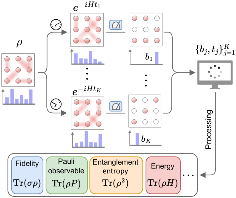
Figure 1: Overview of the Hamiltonian shadow protocol. In each experiment round, the target state $\rho$ evolves with a fixed Hamiltonian and a random time, followed by a computational basis measurement. The data pair of measurement result $b_{j}$ and evolution time $t_{j}$ is recorded on a classical computer to estimate arbitrary properties of $\rho$.

In this work, we address this challenge by presenting the Hamiltonian shadow protocol. This protocol allows for predicting any state property through quench evolution with a single Hamiltonian and different evolution times, as illustrated in Fig. 1. It leverages the inherent randomness in eigen-energies of a single Hamiltonian, eliminating the need for multiple Hamiltonians or ancillary systems. We theoretically prove that computational basis measurements after quantum evolution under a single Hamiltonian can unbiasedly extract arbitrary properties of the target quantum state. Furthermore, the requirements for the quench Hamiltonian are minimal, such as no eigen-energy degeneracy and no computational basis eigenstates, conditions generally met by practical analog systems. Even with a single quench Hamiltonian, both theoretical and numerical analysis demonstrate that the performance of the Hamiltonian shadow is comparable to that of the original shadow with random Clifford unitaries. We apply the proposed method to a Rydberg atoms system with realistic parameter settings and demonstrate its efficacy in estimating several essential physical quantities, including quantum fidelity, local correlation function, and purity. This advancement signifies a substantial leap forward in analog quantum simulation and classical shadow tomography, holding considerable promise for near-term applications.

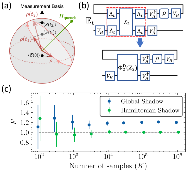
Figure 2: Hamiltonian shadow: intuition, derivation, and unbiased estimation. (a) Geometric intuition of Hamiltonian shadow in a single-qubit Bloch sphere. (b) The tensor network representation of the Hamiltonian shadow map. (c) Performance comparison between two data post-processing methods, the Hamiltonian shadow and the original global shadow, in predicting fidelity. A four-qubit GHZ state is evolved under $e^{-iHt}$ with a single random Hermitian matrix $H$ and random evolution time $t$ and measured in computational basis to get $\ket{b}$. Then, both methods use the dataset of $\{e^{-iHt_{j}},b_{j}\}_{j=1}^{K}$ to construct their fidelity estimators. The error bar indicates a 99.7$\%$ confidence interval (3 standard deviations).

Hamiltonian shadow. The fundamental reason making the state learning with a single Hamiltonian possible is that the measurement basis does not commute with the Hamiltonian. A toy model is illustrated in Fig. 2(a), where an unknown state $\rho$ is a vector in the Bloch sphere, rotating around a known axis determined by the quench Hamiltonian $H_{\text{quench}}$. Based on geometric intuitions, the dynamical trajectory of the $Z$-basis expectation value $\langle Z(t)\rangle$ together with $H_{\text{quench}}$ can recover the vector of $\rho$ [63]. We further ask whether it is possible to fully recover the unknown state $\rho$ by taking single-shot $Z$-basis measurements at different quench times $t$.

Operationally speaking, after quench evolution with $e^{-iHt}$, we take a single-shot measurement, and the state collapses to $\ket{b}$. Then, the classical representation, $\hat{\sigma}=e^{iHt}\outerproduct{b}{b}e^{-iHt}$, contains information of $\rho$. As quantum mechanics is fundamentally linear, the average of the dataset $\{\hat{\sigma}_{j}=e^{iHt_{j}}\outerproduct{b_{j}}{b_{j}}e^{-iHt_{j}}\}_{j}$ is related to $\rho$ through a linear map

$$\mathcal{M}_{H}(\rho)=\mathbb{E}_{t,b}\left[e^{iHt}\outerproduct{b}{b}e^{-iHt}\right].$$ (1)

If the map $\mathcal{M}_{H}$ is invertible, $\hat{\rho}=\mathcal{M}_{H}^{-1}(e^{iHt}\outerproduct{b}{b}e^{-iHt})$ becomes an unbiased estimator of $\rho$. Then, one can use the classical dataset to predict arbitrary state properties, which means that the state learning with a single Hamiltonian is tomography-complete. Specifically, given $\{\hat{\rho}_{j}\}_{j=1}^{K}$, one can construct estimators such as $\frac{1}{K}\sum_{j}\Tr(O\hat{\rho}_{j})$ and $\frac{1}{K(K-1)}\sum_{j\neq k}\Tr[O(\hat{\rho}_{j}\otimes\hat{\rho}_{k})]$ to unbiasedly predict linear and nonlinear properties. This logic aligns with the classical shadow tomography [36]. We thus name this measurement scheme as Hamiltonian shadow and the map $\mathcal{M}_{H}(\cdot)$ as Hamiltonian shadow map.

The Hamiltonian shadow map is uniquely determined by its Choi matrix. Substituting Born’s rule and the spectral decomposition $e^{-iHt}=V_{H}\Lambda_{t}V_{H}^{\dagger}$ with $(\Lambda_{t})_{k,l}=e^{-iE_{k}t}\delta_{k,l}$, we can rewrite the Hamiltonian shadow map as

$$\mathcal{M}_{H}(\rho)=V_{H}\mathcal{N}\left(V_{H}^{\dagger}\rho V_{H}\right)V_{H}^{\dagger}.$$ (2)

From tensor network representation shown in Fig. 2(b), the Choi matrix of $\mathcal{N}$ is $\mathbb{E}_{t}(\Lambda_{t}^{\otimes 2}X_{2}\bar{\Lambda}_{t}^{\otimes 2})$ with $X_{2}=\sum_{b}V_{H}^{\dagger\otimes 2}\outerproduct{bb}{bb}V_{H}^{\otimes 2}$. In general, $\mathcal{N}$ has a complicated form and is hard to invert. However, if eigen-energies of $H$ and evolution time $t$ contain enough randomness to make $\Lambda_{t}$ a random diagonal unitary, the Choi matrix reduces to $\Phi_{2}^{\mathrm{D}}(X_{2})=\sum_{i,j}(X_{2})_{ij,ij}\ket{ij}\bra{ij}+\sum_{i\neq j}(X_{2})_{ij,ji}\ket{ij}\bra{ji}$, where $\Phi_{2}^{\mathrm{D}}(\cdot)$ denotes the second-order integral over random diagonal unitaries. Most elements cancel out due to the integral, and the left ones can be summarized using a much smaller matrix, the post-processing matrix $X_{H}$.

Theorem 1.

For a Hamiltonian $H$, suppose the target state $\rho$ is evolved using $e^{-iHt}$ with a random $t$ and measured in computational basis to get $\ket{b}$. Suppose each element of the ensemble $\{e^{-iHt}\}_{t}$ has a spectral decomposition of $e^{-iHt}=V_{H}\Lambda_{t}V_{H}^{\dagger}$, where $\Lambda_{t}=\sum_{j}e^{i\theta_{j}}\outerproduct{j}{j}$ with each $\theta_{j}$ sampled independently and uniformly from $[0,2\pi)$. Defining $V_{H}^{\mathrm{sq}}=\sum_{i,j}\absolutevalue{(V_{H})_{i,j}}^{2}\outerproduct{i}{j}$, if matrix $X_{H}=(V_{H}^{\mathrm{sq}})^{T}V_{H}^{\mathrm{sq}}$ is invertible and all off-diagonal elements are nonzero, the following expression is the unbiased estimator of $\rho$

$$\hat{\rho}=V_{H}\mathcal{N}^{-1}\left(V_{H}^{\dagger}\hat{\sigma}V_{H}\right)V_{H}^{\dagger},$$ (3)

where $\hat{\sigma}=e^{iHt}\outerproduct{b}{b}e^{-iHt}$ and the action of map $\mathcal{N}^{-1}$ is

$$\mathcal{N}^{-1}(\sigma)=\sum_{i,j}(X_{H}^{-1})_{ij}\sigma_{j,j}\outerproduct{i}{i}+\sum_{i\neq j}(X_{H})_{i,j}^{-1}\sigma_{i,j}\outerproduct{i}{j}.$$ (4)

In the literature, randomized measurements using Hamiltonian evolution either employ multiple chaotic Hamiltonians [22, 57] or ancillary systems [60, 61] to induce randomness. Conversely, we capitalize on the inherent randomness in eigen-energies of a single Hamiltonian $H$. This is more practical as implementing the coherent dynamics $e^{-iHt}$ governed by an intrinsic Hamiltonian $H$ is readily achievable for many analog quantum simulators. Note that directly treating $e^{-iHt}$ as a random Haar unitary and performing the data post-processing of the original global classical shadow will lead to biased estimations. For example, in Fig. 2(c), we show the fidelity estimation with two data post-processing methods, Hamiltonian shadow and global shadow, using the same measurement dataset collected with a single Hamiltonian quench evolution. It is clear that the estimation of Hamiltonian shadow approaches the real value while the global shadow does not.

When dealing with local observables, such as local correlation functions, it becomes advantageous to employ a local version of the Hamiltonian shadow. Assume that the entire system can be segmented into multiple localized patches, and the whole system evolution is $\bigotimes_{p=1}^{N}e^{-iH_{p}t}$ with independent $H_{p}$. The unbiased estimator of $\rho$ can be constructed as

$$\hat{\rho}=\bigotimes_{p=1}^{N}V_{H_{p}}\mathcal{N}^{-1}_{p}(V_{H_{p}}^{\dagger}\hat{\sigma}_{p}V_{H_{p}})V_{H_{p}}^{\dagger},$$ (5)

where $\hat{\sigma}_{p}=e^{iH_{p}t}\outerproduct{b_{p}}{b_{p}}e^{-iH_{p}t}$ and $\mathcal{N}_{p}^{-1}$ is defined in the same way using $X_{H_{p}}$. The local Hamiltonian shadow reduces classical computational resources by only dealing with local-patch Hamiltonians. Besides, the experiment sample complexity is unaffected by the total system size when measuring local observables.

Performance guarantee. The performance of the Hamiltonian shadow protocol largely depends on the Hamiltonian $H$, including its eigenstates and eigen-energies. According to Eq. (4), the Hamiltonian shadow is tomography-complete if the post-processing matrix $X_{H}$, which is determined solely by eigenstates, is invertible, and all off-diagonal elements are non-zero. One common situation where the Hamiltonian shadow becomes tomography-incomplete is when some eigenstates align with the measurement basis, making $X_{H}$ a block-diagonal matrix. Yet, most Hamiltonians without fine-tuning in general satisfy the requirements for $X_{H}$ [64]. The requirement for eigen-energies originates from the assumption that $\Lambda_{t}$ approximates random diagonal unitary. We show that it can be summarized with the non-resonance condition [65, 66], in which no eigen-energy pairs satisfy $E_{a_{1}}+E_{a_{2}}=E_{b_{1}}+E_{b_{2}}$ for $(a_{1},a_{2})\neq(b_{1},b_{2})$ and $(a_{1},a_{2})\neq(b_{2},b_{1})$. Similarly, this condition can generally be satisfied by a quench dynamics Hamiltonian without certain global symmetries [67]. Considering the practical scenario where the evolution time is limited, one may further require eigen-energies of $H$ to have large spacing.

When requirements for eigenstates and eigen-energies are all satisfied, one can efficiently predict many physical properties of the state simultaneously.

Theorem 2.

To estimate expectation values of $M$ arbitrary observables $\{O_{i}\}_{i=1}^{M}$ to $\epsilon$ accuracy with the Hamiltonian shadow protocol, the sample complexity is upper bounded by $K=\mathcal{O}\left(\max_{i}\norm{O_{i}}_{\mathrm{HShadow}}^{2}\log(M)/\epsilon^{2}\right)$, where $\norm{O}_{\mathrm{HShadow}}$ is the Hamiltonian shadow norm determined by $V_{H}$ and $O$.

Details of the Hamiltonian shadow norm can be found in Appendix E. Despite the complicated form of the Hamiltonian shadow norm, which obscures the connection between sample complexities and structures of Hamiltonians, we find that

$$f(O,V_{H})=\sum_{i\neq j}\frac{1}{(X_{H})_{i,j}}\absolutevalue{\bra{i}V_{H}^{\dagger}OV_{H}\ket{j}}^{2}$$ (6)

can approximate $\norm{O}_{\mathrm{HShadow}}^{2}$ well. This formula can be easily extended to nonlinear observables and helps us build intuition between the sample complexity and the Hamiltonian. For example, when eigenstates of $H$ are close to the computational basis, $X_{H}$ approximates a diagonal matrix and $f(O,V_{H})$ increases for having terms of $\frac{1}{(X_{H})_{i,j}}$. It also agrees with the physical intuition since off-diagonal elements of $\rho$ are hard to probe when the unitary evolution $e^{-iHt}$ almost commutes with measurement basis.

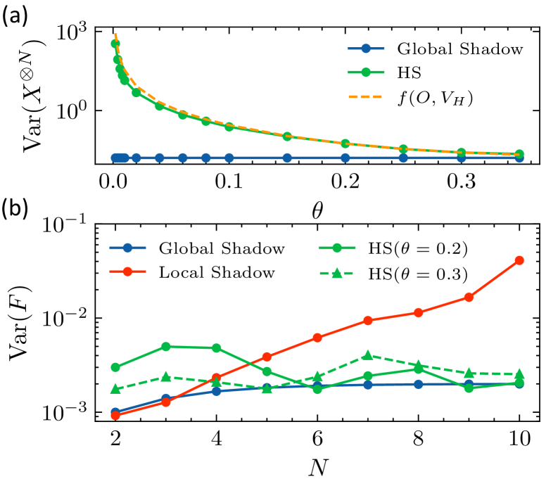
Figure 3: Variance scaling. The evolution unitary is chosen to be $V_{H}\Lambda_{t}V_{H}^{\dagger}=e^{iP\theta}\Lambda_{t}e^{-iP\theta}$, where $\Lambda_{t}$ is a random diagonal unitary, $P$ is a fixed random Hermitian matrix and $\theta$ is a control parameter that determines the difference between measurement basis and eigen-basis of evolution unitary. The number of measurements is $K=1000$, and target states are set to be GHZ states [68]. (a) The variance in estimating $P=X^{\otimes N}$, where $X$ is the Pauli-$X$ operator and $N=4$. (b) The variance scaling with qubit number in estimating fidelity.

To further validate Eq. (6), we choose a Hamiltonian with the diagonalization unitary $V_{H}=e^{iP\theta}$, where $P$ is a fixed Hermitian matrix which is randomly sampled and $\theta$ is a tunable parameter. When $\theta$ approaches zero, eigen-basis of Hamiltonian approaches the measurement basis. While $\theta$ is large, the eigen-basis approaches a random basis. In Fig. 3(a), we use a Pauli observable to show that $f(O,V_{H})$ is indeed a good approximation for the real variance. Another critical observation is that the variance of Hamiltonian shadow gradually approaches the original classical shadow protocol when $\theta$ increases. This can also be observed in Fig. 3(b), where variances of Hamiltonian shadow for estimating fidelity do not increase with qubit number, reproducing a key feature of classical shadow. These observations show that, with a single Hamiltonian, the Hamiltonian shadow generally has a similar ability for state learning compared with the protocol using a set of many independent random unitaries. The similarity between the Hamiltonian shadow and the original shadow can be theoretically verified through the following example [69, 70], which reproduces the variance of original global shadow [36].

Theorem 3.

Suppose the evolution unitary is $U=h^{\otimes N}\Lambda_{t}$, and the measurement result is $\ket{b}$, where $h$ is the Hadamard gate, $N$ is the qubit number, and $\Lambda_{t}$ is random diagonal unitary. Then $2^{N}\overline{\Lambda}_{t}h^{\otimes N}\outerproduct{b}{b}h^{\otimes N}\Lambda_{t}-\mathbb{I}$ is the unbiased estimator of $\rho-\mathrm{diag}(\rho)$. When estimating an observable $O$ with $O_{i,i}=0$ for all $i$, the variance scales as

$$\mathrm{Var}\left(2^{N}\bra{b}h^{\otimes N}\Lambda_{t}O\overline{\Lambda}_{t}h^{\otimes N}\ket{b}\right)$$ (7)

$$\leq\Tr(O^{2})+2\Tr(O^{2}\rho).$$

Applications. The Hamiltonian shadow is applicable to many analog systems, and here we choose Rydberg atom arrays with global laser pulse control as our platform. In the following, we will show how the Hamiltonian shadow with only random atom positions accomplishes three important tasks for quantum many-body physics: (1) measuring quantum fidelity, (2) measuring local stabilizer observable of a topological state, and (3) measuring purity dynamics in quantum thermalization. The platform of the Rydberg atom arrays is one of the leading analog quantum simulators that has realized exotic phases of matter [7]. Using the ground state $\ket{g}$ and the Rydberg state $\ket{r}$ of the neutral atom as a qubit, we model our system with Hamiltonian

$$H=\frac{\Omega}{2}\sum_{j}\left(e^{i\phi}\outerproduct{g_{j}}{r_{j}}+h.c.\right)-\Delta\sum_{j}\hat{n}_{j}+\sum_{j<k}V_{jk}\hat{n}_{j}\hat{n}_{k},$$ (8)

where $\Omega=1.1\times 2\pi\ \mathrm{MHz}$, $\phi=2.1$, and $\Delta=1.2\times 2\pi\ \mathrm{MHz}$ denote the Rabi frequency, laser phase, and detuning of the global driving laser field on atoms that couples the ground and Rydberg state. We will denote $\ket{g}$ as $\ket{0}$, and $\ket{r}$ as $\ket{1}$ afterwards. $V_{jk}=C/|\textbf{x}_{j}-\textbf{x}_{k}|^{6}$ describes the van der Waals interaction between two atoms, where x is the position vector of an atom and the strength $C=2\pi\times 862690\ \mathrm{MHz}\cdot\mu m^{6}$ depends on the Rydberg state . With global control pulses, positions of atoms are randomly set to introduce randomness in eigen-energies of $H$, which is feasible for Rydberg atoms platforms [72]. Specifically, we arrange atoms in a line and set the position of the $j$-th atom to be $j\times D+\delta d_{j}$, where $D=8.781\mu m$ is near the blockade radius, and $\delta d_{j}$ is uniformly and independently sampled from $[-0.488,0.488](\mu m)$. Positions of atoms are kept the same throughout the process of Hamiltonian shadow. This setup is visualized in Fig. 4 (a). Ideally, the evolution time $t$ should be randomly chosen from a long time window $\Delta t=t_{\mathrm{max}}-t_{\mathrm{min}}$ such that $\Lambda_{t}=\text{diag}(e^{-iE_{1}t},e^{-iE_{2}t},\cdots)$ approximates random diagonal unitary. However, considering errors and decoherence in current platforms, $t$ can only be sampled in a limited time window. Thus, the distribution of $\Lambda_{t}$ may deviate from the ideal random diagonal unitary and introduce errors to the Hamiltonian shadow. In the following numerical demonstrations, we will focus on the performance of the Hamiltonian shadow under a limited time window.

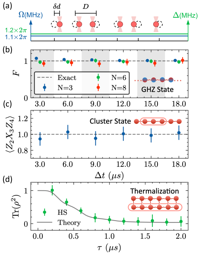
Figure 4: Performances of Hamiltonian shadow with Rydberg atom arrays. (a) The Rydberg atom array setup in Hamiltonian shadow. All atoms are controlled by global pulses ($\Omega,\Delta$) and arranged in a line with random positions. (b) Fidelity estimation with different time windows $\Delta t$ and qubit numbers $N$, where initial states are set to GHZ states. (c) Stabilizer expectation with different time windows, where the initial state is set to be a six-qubit cluster state. (d) Quantum thermalization of a 12-atom system, observed using purity of the 6-atom subsystem. All error bars are estimated with $K=10000$ samples (3 standard deviations) and $t_{\mathrm{min}}=2\mu s$.

For measuring quantum fidelity, we initialize Greenberger–Horne–Zeilinger (GHZ) states with different qubit numbers, $\ket{\psi}=(\ket{010\cdots}+\ket{101\cdots})/2$, which can be prepared with Rydberg atom arrays using blockade mechanism [73]. For measuring local observables, we prepare the underlying state to be the cluster state, a symmetry-protected topological state with $\langle Z_{i-1}X_{i}Z_{i+1}\rangle=1$ [74]. To estimate local stabilizer, $\langle Z_{2}X_{3}Z_{4}\rangle$, we use the local-patch Hamiltonian shadow with a three-qubit Hamiltonian acting on target qubits. Both quantities are challenging to measure with conventional means using global pulse control. In Fig. 4 (b) and (c), we plot fidelity and stabilizer expectations as functions of the time window $\Delta t$. It shows that the Hamiltonian shadow protocol gives precise estimations for both quantities with realistic time windows. Moreover, in Appendix C.1, we show that the bias caused by the limited time window can be fixed by modifying the Hamiltonian shadow map.

Besides linear properties of the quantum state, the Hamiltonian shadow can also predict nonlinear properties given only single-copy access to the quantum state each time. We demonstrate this by observing quantum thermalization under coherent dynamics. Twelve atoms are arranged in a two-leg ladder lattice with initial state $\ket{0}^{\otimes 6}\otimes\ket{1}^{\otimes 6}$, where the upper leg is $\ket{1}^{\otimes 6}$ and lower leg is $\ket{0}^{\otimes 6}$. The atoms are equally separated by $10.733\mu m$ and evolve under the Rydberg Hamiltonian for time $\tau$. With time evolution, entanglement between atoms on the upper and lower legs first grows and then saturates at a maximum value, which is reflected by the purities of atoms on the lower leg for different $\tau$. To estimate purities, after each evolution, we remove atoms on the upper leg and rearrange atoms on the lower leg to the selected random positions as shown in Fig.4 (a) and perform the Hamiltonian shadow protocol. The atom-moving has already been demonstrated in recent experiments [72]. To obtain the precise estimation as shown in Fig.4 (d), we set the maximal evolution time as $t_{\mathrm{max}}=60\mu s$. While compared to fidelity estimation in Fig. 4(b) with the same qubit number, it indicates that a precise estimation of the nonlinear property may require a longer evolution time.

Discussion. Hamiltonian shadow provides a new perspective for linking the information scrambling in quench dynamics with quantum state learning. The performance of Hamiltonian shadow has an intriguing relation with quantum thermalization, such as the non-resonance condition. While developing the Hamiltonian shadow, we proposed many useful tools for the theory of random diagonal unitaries, such as frame potential and diagonal unitary $t$-design [75]. The Hamiltonian shadow still puts a high requirement for the data post-processing. Except for adopting local-patch Hamiltonian shadow, another potential way is to utilize the prior knowledge of $\rho$. For example, if one has a variational ansatz of $\rho$ or $\rho$ is narrowly distributed on eigenstates of $H$, we may avoid using all eigenstates of $H$ in the data post-processing. It is also worth further exploring the applications of Hamiltonian shadow in other analog quantum simulators, such as fermionic and bosonic systems.

Acknowledgement The authors would like to thank Satoya Imai, Otfried Gühne, Richard Kueng, Chao Yin, Soonwon Choi, Christian Kokail, Yi-Zhuang You, Susanne Yelin, Liang Jiang, Katherine Van Kirk, Yanting Teng, Jonathan Kunjummen, Stefan Ostermann, You Zhou, and Hongyi Wang for insightful discussions and suggestions. Zhenhuan Liu is supported by the National Natural Science Foundation of China (Grant No. 12174216). H.Y.H. is grateful for the support from the Harvard Quantum Initiative Fellowship. The code is open-sourced on GitHub.

Appendix A Preliminary

A.1 Tensor Network Representation

We introduce the tensor network representation in this section, which is an important tool for our derivation. In tensor network, a matrix is represented using a box with legs, shown in Fig. 5(a), where the left and right legs stand for the row and column indices, respectively. Different pairs of legs stand for different subsystems of the Hilbert space. Vectors are represented by the triangles with only one-side legs, as shown in Fig. 5(b) and (c). The connection of legs stands for the index contraction, such as the matrix production $AB$ shown in Fig. 5(d) and the trace function shown in Fig. 5(e). If two tensors are listed without connection of legs, like Fig. 5(f), this is the tensor product of two matrices $A\otimes B$.

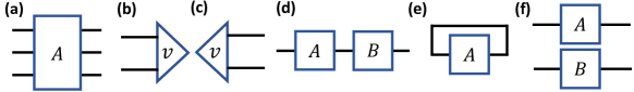
Figure 5: Tensor network representation. (a) A tripartite matrix. (b) A bipartite vector $\ket{v}$. (c) $\bra{v}$. (d) Matrix multiplication. (e) Trace. (f) Tensor product.

Tensor network is good at representing permutation operators, as shown in Fig. 6. A straight line is used to represent the identity operator $\mathbb{I}=\sum_{i}\outerproduct{i}{i}$. A pair of cross lines shown in Fig. 6(b) represents the SWAP operator $S=\sum_{i,j}\outerproduct{ij}{ji}$, which is a second order permutation operator. By adding more lines, we can represent higher-order permutation operators, like shown in Fig. 6(c). Tensor network representations can be used to simplify some calculations. Fig. 6(d) shows a graphical proof of the SWAP trick $\Tr(S\rho^{\otimes 2})=\Tr(\rho^{2})$.

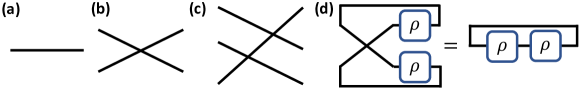
Figure 6: Tensor network representation of permutation operators. (a) The identity operator. (b) The SWAP operator. (c) The third-order cyclic permutation operator. (d) The graphical proof of the SWAP trick.

To facilitate our calculation of random diagonal unitaries, we need to introduce a new kind of labels. We use Fig. 7(a) to represent the matrix of $\sum_{i}\outerproduct{i,\cdots,i}{i,\cdots,i}$, which can be used to contract multiple indices. With this new tool, we can represent matrices which are generated by only preserving some specific elements of original matrices. Take a bipartite matrix, $M=\sum_{i,j,k,l}M_{ij,kl}\outerproduct{ij}{kl}$, as an example, the tensor in Fig. 7(b) gives a diagonal matrix $\sum_{i,j}M_{ij,ij}\outerproduct{ij}{ij}$. The tensor in Fig. 7(c) represents the matrix of $\sum_{i,j}X_{ij,ji}\outerproduct{ij}{ji}$, whose nonzero elements lie in same positions of the SWAP operator $S=\sum_{i,j}\outerproduct{ij}{ji}$. The tensor in Fig. 7(d) is an EPR-like matrix $\sum_{i,j}X_{ii,jj}\outerproduct{ii}{jj}$, whose nonzero elements are in positions of maximally entangled state. Fig. 7(e) is constructed further by the EPR-like matrix, $\sum_{i}X_{ii,ii}\outerproduct{ii}{ii}$.

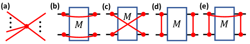
Figure 7: (a) A GHZ-like tensor, $\sum_{i}\outerproduct{i,\cdots,i}{i,\cdots,i}$. (b)-(e), Matrices constructed using the GHZ-like tensor and a bipartite matrix $M=\sum_{i,j}M_{ij,ij}\outerproduct{ij}{ij}$.

Another tool that is important for our derivation is the Choi representation of a linear map. Shown in Fig 8, the output of a linear map $C(\rho)$ can be represented using a higher-dimensional matrix $\mathcal{C}$ contracting with $\rho$. The matrix $\mathcal{C}$ is the Choi matrix of map $C(\cdot)$. In this work, we also refer to $\mathcal{C}^{T_{1}}$ as the Choi matrix of $C(\cdot)$.

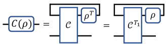
Figure 8: Tensor representation of Choi matrix.

A.2 Random Unitaries

Haar measure random unitary is a uniform distribution in the unitary space, which satisfies

$$\int_{U\sim\mathrm{Haar}}g(UV)dU=\int_{U\sim\mathrm{Haar}}g(U)dU$$ (9)

for any unitary $V$ and function $g(\cdot)$. The Haar-measure random unitary is important for classical shadow due to its relation with permutation operators. According to Schur-Weyl duality, we define the $k$-th order twirling map

$$\Phi_{k}(M)=\int_{U\sim\mathrm{Haar}}U^{\otimes k}MU^{\dagger\otimes k}dU=\sum_{\pi,\sigma\in\mathcal{S}_{k}}\mathrm{Wg}_{\pi,\sigma}\Tr(\hat{W}_{\pi}M)\hat{W}_{\sigma},$$ (10)

where $\mathrm{Wg}$ stands for the Weingarten matrix [76], $\mathcal{S}_{k}$ is the $k$-th order permutation group, $\pi$ and $\sigma$ stand for two elements in $\mathcal{S}_{k}$, and $\hat{W}_{\pi}$ and $\hat{W}_{\sigma}$ are corresponding permutation operators. In this work, we will denote the integral over Clifford group to be $\Phi_{k}^{\mathrm{C}}(\cdot)$ and random diagonal unitaries to be $\Phi_{k}^{\mathrm{D}}(\cdot)$. Specifically, the second order twirling function is

$$\Phi_{2}(M)=\frac{1}{d^{2}-1}\left(\Tr(\mathbb{I}M)\mathbb{I}-\frac{1}{d}\Tr(SM)\mathbb{I}-\frac{1}{d}\Tr(\mathbb{I}M)S+\Tr(SM)S\right)$$ (11)

Instead of integrating over the Haar measure random unitary, we can use the average over a set containing a finite number of unitaries to get the same twirling map

$$\Phi_{k^{\prime}}^{\mathcal{E}_{k}}(M)=\frac{1}{|\mathcal{E}_{k}|}\sum_{U\in\mathcal{E}_{k}}U^{\otimes k^{\prime}}MU^{\dagger\otimes k^{\prime}}=\Phi_{k^{\prime}}(M)$$ (12)

for all $k^{\prime}\leq k$ and matrix $M$. We refer to $\mathcal{E}_{k}$ as the unitary $k$-design. The Clifford group has been proved to be a unitary $3$-design [77].

A.3 Random Diagonal Unitaries

A $d$-dimensional random diagonal unitary is $\Lambda=\mathrm{diag}(e^{i\theta_{1}},\cdots,e^{i\theta_{d}})$, where $\theta_{1},\cdots,\theta_{d}$ are random phases uniformly and independently sampled in $[0,2\pi)$. We define the map of $k$-th order integral over random diagonal unitaries as

$$\Phi_{k}^{\mathrm{D}}(M)=\int_{\Lambda\sim\mathrm{RDU}}\Lambda^{\otimes k}M\overline{\Lambda}^{\otimes k}d\Lambda,$$ (13)

where $\overline{\Lambda}$ is the complex conjugate of $\Lambda$. In this work, $\Phi_{2}^{\mathrm{D}}(\cdot)$ and $\Phi_{3}^{\mathrm{D}}(\cdot)$ will be frequently employed to compute the unbiased estimator and the sample complexity. The action of the second-order map is

$$\Phi_{2}^{\mathrm{D}}(M)=\sum_{i,j}M_{ij,ij}\outerproduct{ij}{ij}+\sum_{i,j}M_{ij,ji}\outerproduct{ij}{ji}-\sum_{i}M_{ii,ii}\outerproduct{ii}{ii}.$$ (14)

We can easily prove this equation using the definition of random diagonal matrix. The element of $\Lambda^{\otimes 2}M\overline{\Lambda}^{\otimes 2}$ is

$$\left(\Lambda^{\otimes 2}M\overline{\Lambda}^{\otimes 2}\right)_{ij,kl}=\Lambda_{i,i}\Lambda_{j,j}\overline{\Lambda}_{k,k}\overline{\Lambda}_{l,l}M_{ij,kl},$$ (15)

which survives from the integral if and only if $i=k$ and $j=l$, or $i=l$ and $j=k$. These elements keep unchanged from the integral while others become zero. This concludes the proof of the second order integral, and the proof for higher order ones are similar. According to Ref. [78], the second and third order integrals can be graphically represented using Fig. 9(a) and (b).

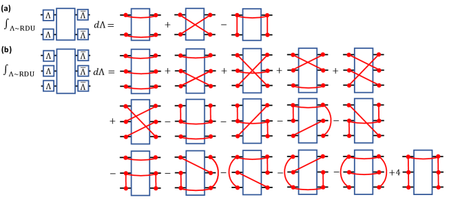
Figure 9: Integrals over random diagonal unitaries. (a) The second-order integral. (b) The third-order integral.

Another important problem is that if the random diagonal unitary has degeneracy, how does the integral change? We consider a specific distribution of diagonal unitary $\mathcal{D}_{1}$. For all $\Lambda$ following the distribution of $\mathcal{D}_{1}$,

$$\Lambda_{j,j}=\begin{cases}e^{i\theta_{j}}&j\neq b\\ \Lambda_{a,a}&j=b\end{cases},$$ (16)

where $\theta_{j}$ is randomly and uniformly sampled from $[0,2\pi)$ and $a\neq b$. Following a similar proof of the second order integral over random diagonal unitaries, more elements can survive from the integral over $\mathcal{D}_{1}$,

$$\int\limits_{\Lambda\sim\mathcal{D}_{1}}\Lambda^{\otimes 2}M\overline{\Lambda}^{\otimes 2}d\Lambda =\sum_{i,j}M_{ij,ij}\outerproduct{ij}{ij}+\sum_{i,j}M_{ij,ji}\outerproduct{ij}{ji}-\sum_{i}M_{ii,ii}\outerproduct{ii}{ii}$$ (17)

$$+\left(\sum_{i}M_{ai,bi}\outerproduct{ai}{bi}+\sum_{i}M_{ai,ib}\outerproduct{ai}{ib}+\sum_{i}M_{ia,bi}\outerproduct{ia}{bi}+\sum_{i}M_{ia,ib}\outerproduct{ia}{ib}+h.c.\right)$$

$$-\left(M_{aa,ba}\outerproduct{aa}{ba}+M_{aa,ab}\outerproduct{aa}{ab}+M_{ba,bb}\outerproduct{ba}{bb}+M_{ab,bb}\outerproduct{ab}{bb}+h.c.\right)$$

$$+(M_{aa,bb}\outerproduct{aa}{bb}+M_{bb,aa}\outerproduct{bb}{aa}).$$

Besides, the second-order degeneracy can also affect the second-order integral. Consider a distribution of diagonal unitaries $\mathcal{D}_{2}$ without first-order degeneracy, whose element $\Lambda$ satisfies

$$\Lambda_{j,j}=\begin{cases}e^{i\theta_{j}}&j\neq b_{2}\\ e^{i(\theta_{a_{1}}+\theta_{a_{2}}-\theta_{b_{1}})}&j=b_{2}\end{cases},$$ (18)

where $(a_{1},a_{2})\neq(b_{1},b_{2})$, $(a_{1},a_{2})\neq(b_{2},b_{1})$, $a_{1}\neq a_{2}$, and $b_{1}\neq b_{2}$. Similarly, every $\theta_{j}$ is sampled uniformly and independently from $[0,2\pi)$. It can be proved that

$$\int\limits_{\Lambda\sim\mathcal{D}_{2}}\Lambda^{\otimes 2}M\overline{\Lambda}^{\otimes 2}d\Lambda=\sum_{i,j}M_{ij,ij}\outerproduct{ij}{ij}+\sum_{i,j}M_{ij,ji}\outerproduct{ij}{ji}-\sum_{i}M_{ii,ii}\outerproduct{ii}{ii}$$ (19)

$$+\left(M_{a_{1}a_{2},b_{1}b_{2}}\outerproduct{a_{1}a_{2}}{b_{1}b_{2}}+M_{a_{2}a_{1},b_{1}b_{2}}\outerproduct{a_{2}a_{1}}{b_{1}b_{2}}+M_{a_{1}a_{2},b_{2}b_{1}}\outerproduct{a_{1}a_{2}}{b_{2}b_{1}}+M_{a_{2}a_{1},b_{2}b_{1}}\outerproduct{a_{2}a_{1}}{b_{2}b_{1}}+h.c.\right).$$

Moreover, if the third-order degeneracy exists, the second-order integral will not be affected. Following the same logic, one can prove that the k-th-order integral only requires that there exists no degeneracy less than k-th order. This tells us that integrating over some other distribution of diagonal unitaries instead of random diagonal unitaries can also give $\Phi_{k}^{\mathrm{D}}(\cdot)$. We can thus introduce the concept of diagonal unitary design.

Similar as the Haar measure random unitary, a set of diagonal unitaries $\mathcal{E}_{k}^{\mathrm{D}}$ is said to be a diagonal unitary $k$ design if

$$\Phi_{k^{\prime}}^{\mathcal{E}^{\mathrm{D}}_{k}}(M)=\frac{1}{|\mathcal{E}^{\mathrm{D}}_{k}|}\sum_{\Lambda\in\mathcal{E}^{\mathrm{D}}_{k}}\Lambda^{\otimes k^{\prime}}M\Lambda^{\dagger\otimes k^{\prime}}=\Phi_{k^{\prime}}^{\mathrm{D}}(M)$$ (20)

for all $k^{\prime}\leq k$ and matrix $M$. We can prove that:

Proposition 1.

Given a set of diagonal unitaries $\mathcal{E}_{k}^{\mathrm{D}}$, whose element $\Lambda=\mathrm{diag}(e^{i\theta_{1}},\cdots,e^{i\theta_{d}})$. If every $\theta$ is sampled uniformly and independently from the set of $\{0,\frac{2\pi}{k+1},\frac{4\pi}{k+1},\cdots,\frac{2k\pi}{k+1}\}$, $\mathcal{E}_{k}^{\mathrm{D}}$ is a diagonal unitary $k$-design.

Proof.

The proof of $k$-design result is equivalent with the proof of the following equality

$$\sum_{\theta\in\{0,\frac{2\pi}{k+1},\cdots,\frac{2k\pi}{k+1}\}}(e^{i\theta})^{k^{\prime}}=0$$ (21)

for all $k^{\prime}\leq k$. Instituting the sum formula for proportional sequence of numbers, we have

$$\sum_{\theta\in\{0,\frac{2\pi}{k+1},\cdots,\frac{2k\pi}{k+1}\}}e^{ik^{\prime}\theta}=\frac{1-e^{i\frac{2k^{\prime}(k+1)}{k+1}\pi}}{1-e^{i\frac{2k^{\prime}}{k+1}\pi}}=0.$$ (22)

∎

To quantify the distance between a given distribution of diagonal unitaries $\mathcal{D}$ and the set of ideal random diagonal unitaries, we introduce the concept of frame potential for diagonal unitaries. Defining $Q_{k}=\int_{U\sim\mathcal{D}}(U^{\dagger})^{\otimes k}\otimes U^{\otimes k}dU-\int_{U\sim\mathrm{RDU}}(U^{\dagger})^{\otimes k}\otimes U^{\otimes k}dU$, we have

$$0\leq\Tr(Q_{k}Q_{k}^{\dagger})=\int_{U\sim\mathcal{D}}\int_{V\sim\mathcal{D}}\absolutevalue{\Tr(U^{\dagger}V)}^{2k}dUdV-2\int_{U\sim\mathcal{D}}\int_{V\sim\mathrm{RDU}}\absolutevalue{\Tr(U^{\dagger}V)}^{2k}dUdV+\int_{U\sim\mathrm{RDU}}\int_{V\sim\mathrm{RDU}}\absolutevalue{\Tr(U^{\dagger}V)}^{2k}dUdV.$$ (23)

Inserting another integral into the second term, we have

$$\int_{U\sim\mathcal{D}}\int_{V\sim\mathrm{RDU}}\absolutevalue{\Tr(U^{\dagger}V)}^{2k}dUdV= \int_{U\sim\mathcal{D}}\int_{V\sim\mathrm{RDU}}\int_{W\sim\mathrm{RDU}}\absolutevalue{\Tr(U^{\dagger}VW^{\dagger})}^{2k}dUdVdW$$ (24)

$$= \int_{U\sim\mathcal{D}}\int_{V\sim\mathrm{RDU}}\int_{W\sim\mathrm{RDU}}\absolutevalue{\Tr\left[(UW)^{\dagger}V\right]}^{2k}dUdVdW$$

$$= \int_{U\sim\mathrm{RDU}}\int_{V\sim\mathrm{RDU}}\absolutevalue{\Tr(U^{\dagger}V)}^{2k}dUdV,$$

where we adopt properties of random diagonal unitaries that a random diagonal unitary can be written as the product of two independent random diagonal unitaries, and $UW$ is a random diagonal unitary if $U$ is a fixed unitary and $W$ is a random diagonal unitary. Therefore, we can define the $k$-th order frame potential of a distribution of diagonal unitary as $F^{(k)}_{\mathcal{D}}=\int_{U\sim\mathcal{D}}\int_{V\sim\mathcal{D}}\absolutevalue{\Tr(U^{\dagger}V)}^{2k}dUdV$ and show that

$$0\leq\Tr(Q_{t}Q_{t}^{\dagger})=\int_{U\sim\mathcal{D}}\int_{V\sim\mathcal{D}}\absolutevalue{\Tr(U^{\dagger}V)}^{2k}dUdV-\int_{U\sim\mathrm{RDU}}\int_{V\sim\mathrm{RDU}}\absolutevalue{\Tr(U^{\dagger}V)}^{2k}dUdV=F^{(k)}_{\mathcal{D}}-F^{(k)}_{\mathrm{RDU}}.$$ (25)

This means that the $k$-th order frame potential of a diagonal unitary distribution is always larger than the frame potential of the distribution of ideal random diagonal unitaries. Only when the distribution is a diagonal unitary $k$-design, these two frame potentials are equivalent. Thus, we can use $F_{\mathcal{D}}^{(k)}$ to show the difference between $\mathcal{D}$ and diagonal unitary $k$-design.

Another thing we need to calculate is the value of frame potential for random diagonal unitaries. Denoting a random diagonal unitary by $U=\mathrm{diag}\left(z_{1},\cdots,z_{d}\right)$, where these terms satisfy $\mathbb{E}\left[z_{i}^{n}(z_{j}^{*})^{m}\right]=\delta_{n,m}\delta_{i,j}$, we have

$$F_{\mathrm{RDU}}^{(k)}= \int_{U\sim\mathrm{RDU}}\int_{V\sim\mathrm{RDU}}\absolutevalue{\Tr(U^{\dagger}V)}^{2k}dUdV$$ (26)

$$= \int_{U\sim\mathrm{RDU}}\absolutevalue{\Tr(U)}^{2k}dU$$

$$= \mathbb{E}\left[(z_{1}+\cdots+z_{d})^{k}(z_{1}^{*}+\cdots+z_{d}^{*})^{k}\right]$$

$$= \mathbb{E}\left(\sum_{n_{1},\cdots,n_{d}\in\mathbb{N},n_{1}+\cdots+n_{d}=k}\binom{k}{n_{1},\cdots,n_{d}}z_{1}^{n_{1}}\cdots z_{d}^{n_{d}}\right)\left(\sum_{n_{1}^{\prime},\cdots,n_{d}^{\prime}\in\mathbb{N},n_{1}^{\prime}+\cdots+n_{d}^{\prime}=k}\binom{k}{n_{1}^{\prime},\cdots,n_{d}^{\prime}}(z_{1}^{n_{1}^{\prime}}\cdots z_{d}^{n_{d}^{\prime}})^{*}\right)$$

$$= \sum_{n_{1},\cdots,n_{d}\in\mathbb{N},n_{1}+\cdots+n_{d}=k}\binom{k}{n_{1},\cdots,n_{d}}^{2}.$$

In this work, we mainly focus on $k=1,2,3$, the frame potentials can be calculated to be

$$F_{\mathrm{RDU}}^{(1)}=d\ ,\ F_{\mathrm{RDU}}^{(2)}=2d^{2}-d\ ,\ F_{\mathrm{RDU}}^{(3)}=6d^{3}-9d^{2}+4d.$$ (27)

Appendix B Brief Introduction to Classical Shadow

In this section, we give a brief and graphical review of the derivation of original shadow map and its variance. This review will be helpful for our construction of Hamiltonian shadow protocol.

Here we focus on the original shadow protocol with global random Clifford gates, which can be easily extended to local version. One first acts a global random unitary $U$, which is sampled from the Haar measure random unitary or a Clifford group, on the target quantum state $\rho$. Then one performs the projective measurement on the evolved state to get the measurement result $\ket{b}$. The shadow map is defined as

$$\mathcal{M}(\rho)=\mathbb{E}_{U,b}\left(U^{\dagger}\outerproduct{b}{b}U\right)=\mathbb{E}_{U}\left(\sum_{b}\bra{b}U\rho U^{\dagger}\ket{b}U^{\dagger}\outerproduct{b}{b}U\right).$$ (28)

Using tensor network, we can graphically represent the shadow map as

$$\mathcal{M}(\rho)= \mathbb{E}_{U}\left(\sum_{b}\begin{tabular}[]{c}\includegraphics[scale={0.25}]{figure/shadow_map1.pdf}\end{tabular}\right)$$ (29)

$$= \mathbb{E}_{U}\left(\sum_{b}\begin{tabular}[]{c}\includegraphics[scale={0.25}]{figure/shadow_map2.pdf}\end{tabular}\right)=\mathbb{E}_{U}\left(\begin{tabular}[]{c}\includegraphics[scale={0.25}]{figure/shadow_map3.pdf}\end{tabular}\right),$$

where $X_{2}=\sum_{b}\outerproduct{bb}{bb}$. Combining the second order twirling function in Eq. (11) with the property of $X_{2}$, $\Tr(\mathbb{I}X_{2})=\Tr(SX_{2})=d$, we have

$$\mathcal{M}(\rho)=\begin{tabular}[]{c}\includegraphics[scale={0.25}]{figure/shadow_map4.pdf}\end{tabular}=\frac{d-1}{d^{2}-1}\left(\begin{tabular}[]{c}\includegraphics[scale={0.25}]{figure/shadow_map5.pdf}\end{tabular}\right)=\frac{1}{d+1}\left(\mathbb{I}+\rho\right).$$ (30)

Therefore, the unbiased estimator of $\rho$ constructed by global shadow is

$$\hat{\rho}=\mathcal{M}^{-1}\left(U^{\dagger}\outerproduct{b}{b}U\right)=(d+1)U^{\dagger}\outerproduct{b}{b}U-\mathbb{I},$$ (31)

and the unbiased estimator of $\Tr(O\rho)$ is $\hat{o}=\Tr(O\hat{\rho})=(d+1)\bra{b}UOU^{\dagger}\ket{b}-\Tr(O)$. The unbiasedness of $\hat{\rho}$ is shown by $\mathbb{E}_{U,b}\left(\hat{\rho}\right)=\mathcal{M}^{-1}\left[\mathbb{E}_{U,b}\left(U^{\dagger}\outerproduct{b}{b}U\right)\right]=\mathcal{M}^{-1}[\mathcal{M}(\rho)]=\rho$.

Now we spend some time to see how to derive the variance of shadow estimator $\hat{o}$. By definition,

$$\mathrm{Var}(\hat{o})= \mathbb{E}_{U,b}\left[(d+1)\bra{b}UOU^{\dagger}\ket{b}-\Tr(O)\right]^{2}-\Tr(O\rho)^{2}$$ (32)

$$= \mathbb{E}_{U,b}\left[(d+1)^{2}\bra{b}UOU^{\dagger}\ket{b}^{2}\right]-2\Tr(O)\left[\Tr(O\rho)+\Tr(O)\right]+\Tr(O)^{2}-\Tr(O\rho)^{2}$$

$$= \mathbb{E}_{U,b}\left[(d+1)^{2}\bra{b}UOU^{\dagger}\ket{b}^{2}\right]-2\Tr(O)\Tr(O\rho)-\Tr(O)^{2}-\Tr(O\rho)^{2}.$$

We can expand the first term as

$$\mathbb{E}_{U,b}\left[(d+1)^{2}\bra{b}UOU^{\dagger}\ket{b}^{2}\right]=(d+1)^{2}\mathbb{E}_{U}\left[\sum_{b}\bra{b}U\rho U^{\dagger}\ket{b}\bra{b}UOU^{\dagger}\ket{b}^{2}\right]$$ (33)

$$= (d+1)^{2}\mathbb{E}_{U}\left(\sum_{b}\begin{tabular}[]{c}\includegraphics[scale={0.25}]{figure/shadow_map6.pdf}\end{tabular}\right)=(d+1)^{2}\begin{tabular}[]{c}\includegraphics[scale={0.25}]{figure/shadow_map7.pdf}\end{tabular}=\frac{d+1}{d+2}\sum_{\pi\in\mathcal{S}_{3}}\begin{tabular}[]{c}\includegraphics[scale={0.25}]{figure/shadow_map8.pdf}\end{tabular}$$

$$= \frac{d+1}{d+2}\left[\Tr(O)^{2}+\Tr(O^{2})+2\Tr(O\rho)\Tr(O)+2\Tr(O^{2}\rho)\right],$$

where grey dashed lines represent the trace function, $X_{3}=\sum_{b}\outerproduct{bbb}{bbb}$, $\mathcal{S}_{3}$ is the third-order permutation group, and $\Phi_{3}^{\mathrm{C}}(\cdot)$ is the third-order twirling map over global Clifford group whose explicit form can be found in Ref. [76]. The last but one equal sign is due to the fact of $\tr(W_{\pi}X_{3})=d$ for all $\pi\in\mathcal{S}_{3}$. Combining Eq. (32) and Eq. (33), we have

$$\mathrm{Var}(\hat{o})=\frac{d+1}{d+2}\left[\Tr(O^{2})+2\Tr(O^{2}\rho)\right]-\frac{1}{d+2}\left[2\Tr(O)\Tr(O\rho)+\Tr(O)^{2}\right]-\Tr(O\rho)^{2}\leq 3\Tr(O^{2}),$$ (34)

where we use the relation of $\Tr(O^{2}\rho)\leq\Tr(O^{2})$. While, except for some special cases like $O=\rho=\outerproduct{\psi}{\psi}$, $\Tr(O^{2}\rho)$ is normally much smaller than $\Tr(O^{2})$. So, we obtain the key observation that the leading term of variance is

$$\Tr\left[\left(O^{\otimes 2}\otimes\rho\right)\left(S\otimes\mathbb{I}\right)\right]=\begin{tabular}[]{c}\includegraphics[scale={0.25}]{figure/shadow_map9.pdf}\end{tabular},$$ (35)

which stands for the indices contraction between two observable matrices. This will provide us important intuition when we calculate the variance of our Hamiltonian shadow.

Appendix C Hamiltonian Shadow Map

In this section, we will derive the unbiased Hamiltonian shadow estimators for cases of global and local Hamiltonian evolution, shown in Fig. 10. We will start from the global case and extend it to the local case.

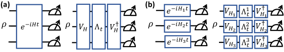
Figure 10: The Hamiltonian evolution with different times. (a) Global Hamiltonian. (b) Local Hamiltonian.

In a single round of experiment, the state $\rho$ will be evolved using a unitary $e^{-iHt}$ with a fixed Hamiltonian and a random $t$. This unitary can be decomposed as $V_{H}\Lambda_{t}V_{H}^{\dagger}$, where $V_{H}$ is a fixed unitary that is independent of $t$ and $\Lambda_{t}=\mathrm{diag}(e^{-iE_{1}t},\cdots,e^{-iE_{d}t})$. As shown in Fig. 10, after each experiment, suppose the measurement outcome is $b$, the shadow map is

$$\mathcal{M}_{H}(\rho)=\mathbb{E}_{b,t}\left(e^{iHt}\outerproduct{b}{b}e^{-iHt}\right)=V_{H}\left[\mathbb{E}_{b,t}\left(\overline{\Lambda}_{t}V_{H}^{\dagger}\outerproduct{b}{b}V_{H}\Lambda_{t}\right)\right]V_{H}^{\dagger}$$ (36)

Substituting the Born’s rule, we have

$$\mathcal{M}_{H}(\rho)= \mathbb{E}_{t}\left(\sum_{b}\bra{b}e^{-iHt}\rho e^{iHt}\ket{b}e^{iHt}\outerproduct{b}{b}e^{-iHt}\right)$$ (37)

$$= \mathbb{E}_{t}\left(\sum_{b}\begin{tabular}[]{c}\includegraphics[scale={0.25}]{figure/derivation1.pdf}\end{tabular}\right)$$

$$= \mathbb{E}_{t}\left(\sum_{b}\begin{tabular}[]{c}\includegraphics[scale={0.25}]{figure/derivation2.pdf}\end{tabular}\right).$$

By slightly abusing the indicators, we define $X_{2}=\sum_{b}(V_{H}^{\dagger})^{\otimes 2}\outerproduct{bb}{bb}V_{H}^{\otimes 2}$ hereafter. The specific form of Hamiltonian shadow map highly depends on the property of $\Lambda_{t}$. According to Eq. (17) and Eq. (19), correlations among different eigenvalues of $H$, like the first and second-order degeneracy, and limited evolution time can significantly affect $\mathcal{M}_{H}$ and sometimes can even make it irreversible. We will discuss this in detail later. Assuming $\Lambda_{t}$ to be an ideal random diagonal unitaries, we have

$$\mathcal{M}_{H}(\rho)= \mathbb{E}_{t}\left(\begin{tabular}[]{c}\includegraphics[scale={0.25}]{figure/derivation3.pdf}.\end{tabular}\right)=\begin{tabular}[]{c}\includegraphics[scale={0.25}]{figure/derivation4.pdf}\end{tabular}$$ (38)

$$= \begin{tabular}[]{c}\includegraphics[scale={0.25}]{figure/derivation5.pdf}\end{tabular}$$

$$= V_{H}\mathcal{N}(V_{H}^{\dagger}\rho V_{H})V_{H}^{\dagger},$$

where the Choi matrix of $\mathcal{N}$ is $\Phi_{2}^{\mathrm{D}}(X_{2})$. Notice that whether this classical shadow protocol is tomography-complete depends on the reversibility of $\mathcal{N}$ and the Hamiltonian shadow estimator is

$$\hat{\rho}=\mathcal{M}_{H}^{-1}\left(e^{iHt}\outerproduct{b}{b}e^{-iHt}\right)=V_{H}\mathcal{N}^{-1}\left(V_{H}^{\dagger}e^{iHt}\outerproduct{b}{b}e^{-iHt}V_{H}\right)V_{H}^{\dagger}=V_{H}\mathcal{N}^{-1}\left(\overline{\Lambda}_{t}V_{H}^{\dagger}\outerproduct{b}{b}V_{H}\Lambda_{t}\right)V_{H}^{\dagger}.$$ (39)

Generally speaking, it is hard to invert a general linear map. To ease the computational complexity, we need to utilize the structure of $\Phi_{2}^{\mathrm{D}}(X_{2})$. Using the second-order integral over random diagonal unitaries, Eq. (14), the action of map $\mathcal{N}$ can be simplified as

$$\mathcal{N}(\sigma)= \sum_{i,j}(X_{2})_{ij,ij}\sigma_{i,i}\outerproduct{j}{j}+\sum_{i,j}(X_{2})_{ij,ji}\sigma_{j,i}\outerproduct{j}{i}-\sum_{i}(X_{2})_{ii,ii}\sigma_{i,i}\outerproduct{i}{i}$$ (40)

$$= \sum_{j}\left(\sum_{i}(X_{2})_{ij,ij}\sigma_{i,i}\right)\outerproduct{j}{j}+\sum_{i\neq j}(X_{2})_{ij,ji}\sigma_{j,i}\outerproduct{j}{i}.$$

It is shown that only a small part of elements of $X_{2}$ contributes to the definition of map $\mathcal{N}$. We thus define a new matrix $X_{H}$ with $(X_{H})_{i,j}=(X_{2})_{ji,ji}$. Substituting the definition of $X_{2}$, we have

$$(X_{H})_{i,j} =(X_{2})_{ji,ji}=\sum_{b}\bra{ji}(V_{H}^{\dagger})^{\otimes 2}\outerproduct{bb}{bb}V_{H}^{\otimes 2}\ket{ji}=\sum_{b}|(V_{H})_{i,b}|^{2}|(V_{H})_{j,b}|^{2}=(X_{2})_{ij,ij}=(X_{H})_{j,i},$$ (41)

$$(X_{2})_{ij,ji} =\sum_{b}\bra{ij}(V_{H}^{\dagger})^{\otimes 2}\outerproduct{bb}{bb}V_{H}^{\otimes 2}\ket{ji}=\sum_{b}|(V_{H})_{i,b}|^{2}|(V_{H})_{j,b}|^{2}=(X_{2})_{ji,ij}=(X_{H})_{i,j}.$$

Then, the map $\mathcal{N}$ can be further simplified as

$$\mathcal{N}(\sigma)=\sum_{i}\left(\sum_{j}(X_{H})_{i,j}\sigma_{j,j}\right)\outerproduct{i}{i}+\sum_{i\neq j}(X_{H})_{i,j}\sigma_{i,j}\outerproduct{i}{j}.$$ (42)

The inverse map can thus be written as

$$\mathcal{N}^{-1}(\sigma)=\sum_{i}\left(\sum_{j}(X_{H}^{-1})_{i,j}\sigma_{j,j}\right)\outerproduct{i}{i}+\sum_{i\neq j}(X_{H})_{i,j}^{-1}\sigma_{i,j}\outerproduct{i}{j}.$$ (43)

Notice that the matrix $X_{H}$ is related with $V_{H}$ in a more straightforward way. Defining $V_{H}^{\mathrm{sq}}=\sum_{i,j}\absolutevalue{(V_{H})_{i,j}}^{2}\outerproduct{i}{j}$, we can prove that

$$X_{H}=\sum_{i,j}\left(\sum_{b}\absolutevalue{(V_{H})_{b,i}}^{2}\absolutevalue{(V_{H})_{b,j}}^{2}\right)\outerproduct{i}{j}=(V_{H}^{\mathrm{sq}})^{T}V_{H}^{\mathrm{sq}}.$$ (44)

Based on Eq. (43), we can derive the conditions under which the Hamiltonian shadow map is reversible. Firstly, the matrix $X_{H}$ needs to be invertible, which makes sure that diagonal elements of $V_{H}^{\dagger}\rho V_{H}$ can be estimated. Secondly, off-diagonal terms of $X_{H}$ cannot be zero, which ensures that all off-diagonal terms of $V_{H}^{\dagger}\rho V_{H}$ can be estimated. Note that, if some condition is not satisfied, although the shadow map is not invertible, we can still estimate some elements of $V_{H}^{\dagger}\rho V_{H}$ by taking the peudo-inverse of $\mathcal{N}$.

These conclusions can be easily extended to local version, where the evolution unitary is $\bigotimes_{p=1}^{N}e^{-iH_{p}t}$. We assume all the single-patch Hamiltonians $H_{p}$ are independent and the evolution time $t$ is also randomly sampled. Denoting the measurement result as $\bigotimes_{p=1}^{N}\outerproduct{b_{p}}{b_{p}}$, the corresponding shadow map is

$$\mathbb{E}_{t}\left(\bigotimes_{p=1}^{N}\mathbb{E}_{b_{p}}e^{iH_{p}t}\outerproduct{b_{p}}{b_{p}}e^{-iH_{p}t}\right)=\mathbb{E}_{t}\left(\begin{tabular}[]{c}\includegraphics[scale={0.22}]{figure/derivation6.pdf}\end{tabular}\right)=\begin{tabular}[]{c}\includegraphics[scale={0.22}]{figure/derivation7.pdf}\end{tabular}=\left(\bigotimes_{p=1}^{N}\mathcal{M}_{H_{p}}\right)(\rho),$$ (45)

where $X_{2}^{p}=\sum_{b_{p}}V_{H_{p}}^{\dagger\otimes 2}\outerproduct{b_{p}b_{p}}{b_{p}b_{p}}V_{H_{p}}^{\otimes 2}$. It can be similarly proved that the following gives the unbiased estimator of $\rho$

$$\hat{\rho}=\bigotimes_{p=1}^{N}V_{H_{p}}\mathcal{N}_{p}^{-1}\left(\overline{\Lambda}_{t}^{p}V_{H_{p}}^{\dagger}\outerproduct{b_{p}}{b_{p}}V_{H_{p}}\Lambda_{t}^{p}\right)V_{H_{p}}^{\dagger},$$ (46)

where $\mathcal{N}_{p}$ is defined in the same way as the global version using the single-patch Hamiltonian $H_{p}$.

Note that the tensor product structure of the Hamiltonian shadow map, i.e. the tensor product structure of Choi matrix, highly depends on the requirement that all $\Lambda_{t}^{p}$ are mutually independent. If this condition is not satisfied, such as some eigenvalues of $H_{p}$ are equivalent with some eigenvalues of $H_{p^{\prime}}$, we will fail to get a Choi matrix with a tensor product structure. Considering the difficulty in choosing different local Hamiltonians for some analog systems, one can also set different evolution times $t_{p}$ for different patches to achieve a same target.

C.1 Limited Evolution Time

Derivations till now are based on the assumption that $\Lambda_{t}$ is an ideal random diagonal unitary. While, in some cases where the time period $t\in[t_{\mathrm{min}},t_{\mathrm{max}}]$ is not long enough, $\Lambda_{t}$ has certain distance with ideal random diagonal unitary and $X_{H}$ cannot fully describe the action of $\mathcal{N}$. We need to recalculate the integral of $\Phi_{2}^{\mathrm{D}}(X_{2})$ as

$$\Phi_{2}^{\mathrm{\Delta t}}(X_{2})=\frac{1}{t_{\mathrm{max}}-t_{\mathrm{min}}}\int_{t_{\mathrm{min}}}^{t_{\mathrm{max}}}\Lambda_{t}^{\otimes 2}X_{2}\overline{\Lambda}_{t}^{\otimes 2}dt,$$ (47)

where $\Lambda_{t}=\mathrm{diag}(e^{-iE_{1}t},e^{-iE_{1}t},\cdots,e^{-iE_{d}t})$. Elements of $\Phi_{2}^{\Delta t}(X_{2})_{ij,ij}$ and $\Phi_{2}^{\Delta t}(X_{2})_{ij,ji}$ are the same as $\Phi_{2}^{\mathrm{D}}(X_{2})_{ij,ij}$ and $\Phi_{2}^{\mathrm{D}}(X_{2})_{ij,ji}$ as phases cancel out. While, other terms are not zero when $\Delta t=t_{\mathrm{max}}-t_{\mathrm{min}}$ is finite. This can be proved from the integral,

$$\Phi_{2}^{\Delta t}(X_{2})_{ij,kl}= \frac{1}{t_{\mathrm{max}}-t_{\mathrm{min}}}\int_{t_{\mathrm{min}}}^{t_{\mathrm{max}}}e^{-i(E_{i}+E_{j}-E_{k}-E_{l})t}(X_{2})_{ij,kl}dt$$ (48)

$$= \frac{(X_{2})_{ij,kl}}{i(t_{\mathrm{max}}-t_{\mathrm{min}})(E_{k}+E_{l}-E_{i}-E_{j})}\left(e^{-i(E_{i}+E_{j}-E_{k}-E_{l})t_{\mathrm{max}}}-e^{-i(E_{i}+E_{j}-E_{k}-E_{l})t_{\mathrm{min}}}\right).$$

Thus, except for cases where $E_{i}+E_{j}=E_{k}+E_{l}$, other matrix elements of $\Phi_{2}^{\Delta t}(X_{2})$ all decrease with the time period $\Delta t$. While for finite $\Delta t$, these elements are normally not zero.

The first information we get from Eq. (48) is that the only requirement for eigenvalues of $H$ is that except for $(i,j)=(k,l)$ and $(i,j)=(l,k)$, $E_{i}+E_{j}\neq E_{k}+E_{l}$. In addition to this, other correlations of different eigenvalues do not affect the unbiasedness of Hamiltonian shadow when $\Delta t$ is sufficiently large. This is because when $E_{i}+E_{j}\neq E_{k}+E_{l}$, $[\Phi_{2}^{\Delta t}(X_{2})]_{ij,kl}$ will decay to zero when $\Delta t\to\infty$. Such conclusion also meets our analysis in Appendix A.3, stated that the degeneracy higher than order two does not affect the second-order integral. Besides, when $\Delta t$ is finite, we can adjust the post-processing of Hamiltonian shadow protocol to remove the bias. In this case, the matrix $X_{H}$ cannot fully describe the map $\mathcal{N}$, as the Choi matrix of $\mathcal{N}$ is replaced from $\Phi_{2}^{\mathrm{D}}(X_{2})$ to $\Phi_{2}^{\Delta t}(X_{2})$. While, combining Eq. (48) and information of $\Delta t$ and $H$, we can still numerically determine the map $\mathcal{N}$ and its inverse $\mathcal{N}^{-1}$. Then, following the same logic, Eq. (39) with a new definition of $\mathcal{N}^{-1}$ can give the unbiased estimator of $\rho$.

In the case of finite time scale, we can also derive an analytical expression of the frame potential, which can be used to show the difference between $\Lambda_{t}$ and the ideal random diagonal unitary. Assuming $z_{j}=e^{-iE_{j}(t_{2}-t_{1})}$ for $1\leq j\leq d$, the $k$-th order frame potential is

$$F^{(k)}_{\Delta t}=\mathbb{E}_{t_{1},t_{2}}\absolutevalue{\Tr(\overline{\Lambda}_{t_{1}}\Lambda_{t_{2}})}^{2k}$$ (49)

$$= \mathbb{E}_{t_{1},t_{2}}\left(\sum_{n_{1},\cdots,n_{d}\in\mathbb{N},n_{1}+\cdots+n_{d}=k}\binom{k}{n_{1},\cdots,n_{d}}z_{1}^{n_{1}}\cdots z_{d}^{n_{d}}\right)\left(\sum_{n_{1}^{\prime},\cdots,n_{d}^{\prime}\in\mathbb{N},n_{1}^{\prime}+\cdots+n_{d}^{\prime}=k}\binom{k}{n_{1}^{\prime},\cdots,n_{d}^{\prime}}(z_{1}^{n_{1}^{\prime}}\cdots z_{d}^{n_{d}^{\prime}})^{*}\right)$$

$$= \frac{1}{(t_{\max}-t_{\min})^{2}}\sum_{n_{1},\cdots,n_{d}\in\mathbb{N},n_{1}+\cdots+n_{d}=k}\sum_{n_{1}^{\prime},\cdots,n_{d}^{\prime}\in\mathbb{N},n_{1}^{\prime}+\cdots+n_{d}^{\prime}=k}\binom{k}{n_{1},\cdots,n_{d}}\binom{k}{n_{1}^{\prime},\cdots,n_{d}^{\prime}}\int_{t_{\min}}^{t_{\max}}\int_{t_{\min}}^{t_{\max}}z_{1}^{n_{1}-n_{1}^{\prime}}\cdots z_{d}^{n_{d}-n_{d}^{\prime}}dt_{1}dt_{2}$$

$$= \frac{1}{(t_{\max}-t_{\min})^{2}}\sum_{n_{1},\cdots,n_{d}}\sum_{n_{1}^{\prime},\cdots,n_{d}^{\prime}}\binom{k}{n_{1},\cdots,n_{d}}\binom{k}{n_{1}^{\prime},\cdots,n_{d}^{\prime}}\int_{t_{\min}}^{t_{\max}}\int_{t_{\min}}^{t_{\max}}e^{-i(n_{1}-n_{1}^{\prime})E_{1}(t_{2}-t_{1})}\cdots e^{-i(n_{d}-n_{d}^{\prime})E_{d}(t_{2}-t_{1})}dt_{1}dt_{2}$$

$$= \sum_{n_{1},\cdots,n_{d}}\sum_{n_{1}^{\prime},\cdots,n_{d}^{\prime}}\binom{k}{n_{1},\cdots,n_{d}}\binom{k}{n_{1}^{\prime},\cdots,n_{d}^{\prime}}\absolutevalue{\frac{\left(e^{i\left(\sum_{j=1}^{d}(n_{j}^{\prime}-n_{j})E_{j}\right)t_{\max}}-e^{i\left(\sum_{j=1}^{d}(n_{j}^{\prime}-n_{j})E_{j}\right)t_{\min}}\right)}{i(t_{\max}-t_{\min})\sum_{j=1}^{d}(n_{j}^{\prime}-n_{j})E_{j}}}^{2},$$

where we use $\sum_{n_{1},\cdots,n_{d}}$ to simplify the notation of $\sum_{n_{1},\cdots,n_{d}\in\mathbb{N},n_{1}+\cdots+n_{d}=k}$. Lets consider a practical Hamiltonian $H=\sum_{i}H_{i}$, where each $H_{i}$ has small locality. Normally speaking, eigenvalues of the Hamiltonian scale polynomially while the number of eigenvalues scales exponentially with the qubit number. If we fix the time scale $\Delta t=t_{\max}-t_{\min}$ and $k$, the value of $\binom{k}{n_{1},\cdots,n_{d}}\binom{k}{n_{1}^{\prime},\cdots,n_{d}^{\prime}}\absolutevalue{\frac{\left(e^{i\left(\sum_{j=1}^{d}(n_{j}^{\prime}-n_{j})E_{j}\right)t_{\max}}-e^{i\left(\sum_{j=1}^{d}(n_{j}^{\prime}-n_{j})E_{j}\right)t_{\min}}\right)}{i(t_{\max}-t_{\min})\sum_{j=1}^{d}(n_{j}^{\prime}-n_{j})E_{j}}}^{2}$ decays only polynomially with qubit number. However, the number of summation terms contributing to the $k$-th order frame potential scales asymptotically $2^{2kN}$ with qubit number. Compared with $2^{kN}$ terms left in the frame potential of random diagonal unitary, Eq. (26), the frame potential of finite time will be exponentially larger than the ideal random diagonal unitary.

Taking the Rydberg atom array Hamiltonian as an example,

$$H=\frac{\Omega}{2}\sum_{j}\left(e^{i\phi}\outerproduct{g_{j}}{r_{j}}+h.c.\right)-\Delta\sum_{j}\hat{n}_{j}+\sum_{j<k}V_{jk}\hat{n}_{j}\hat{n}_{k},$$ (50)

we follow the same parameter setting as the main context and fix the time scale $\Delta t=20\mu s$. The evolution unitary can be decomposed as $e^{-iHt}=V_{H}\Lambda_{t}V_{H}^{\dagger}$ and $\Lambda_{t}$ follows a finite-time random diagonal unitary distribution. We numerically calculate the scaling of frame potential of $\Lambda_{t}$ with the qubit number, shown in Fig. 11. It is obvious that the finite-time frame potential is exponentially larger than the frame potential of ideal random diagonal unitary. Besides, the scaling slope becomes larger when $k$ increases, which matches our prediction. However, as shown in main context, the Hamiltonian shadow using the Rydberg atom array Hamiltonian with $\Delta t\leq 20\mu s$ performs well in estimating observables. Thus, it is still an open problem to determine the relation between the frame potential and performance of Hamiltonian shadow.

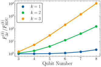
Figure 11: The scaling of finite-time frame potential with qubit number, with different $k$.

Appendix D Case Studies

D.1 Single-Qubit Case

In this section, we use the simplest example, the single-qubit case, to show how Hamiltonian shadow works and give the intuition of the factors influencing its performance. As $e^{-iHt}\rho e^{iHt}=V_{H}\Lambda_{t}V_{H}^{\dagger}\rho V_{H}\overline{\Lambda}_{t}V_{H}^{\dagger}$ and $V_{H}$ is a fixed unitary which is independent of $t$, we can define $\rho_{H}=V_{H}^{\dagger}\rho V_{H}$ and regard the whole process as $\rho_{H}$ under the evolution of $V_{H}\Lambda_{t}$. The complete learning of $\rho$ is equivalent with the complete learning of $\rho_{H}$.

Considering a single-qubit quantum state $\rho_{H}=\begin{bmatrix}\rho_{00}&\rho_{01}\\ \rho_{10}&\rho_{11}\end{bmatrix}$, we evolve it using a random diagonal unitary $\Lambda_{t}=\mathrm{diag}(e^{i\theta_{1}},e^{i\theta_{2}})$ followed by a fixed unitary $V_{H}=\begin{bmatrix}\cos{\phi}&\sin{\phi}\\ -\sin{\phi}&\cos{\phi}\end{bmatrix}=\begin{bmatrix}c&s\\ -s&c\end{bmatrix}$. After such evolution, the density matrix will become

$$V_{H}\Lambda_{t}\rho_{H}\overline{\Lambda}_{t}V_{H}^{\dagger} =\begin{bmatrix}ce^{i\theta_{1}}&se^{i\theta_{2}}\\ -se^{i\theta_{1}}&ce^{i\theta_{2}}\end{bmatrix}\rho\begin{bmatrix}ce^{-i\theta_{1}}&-se^{-i\theta_{1}}\\ se^{-i\theta_{2}}&ce^{-i\theta_{2}}\end{bmatrix}$$ (51)

$$=\begin{bmatrix}c^{2}\rho_{00}+s^{2}\rho_{11}+cse^{i(\theta_{2}-\theta_{1})}\rho_{10}+cse^{i(\theta_{1}-\theta_{2})}\rho_{01}&cs(\rho_{11}-\rho_{00})+c^{2}e^{i(\theta_{1}-\theta_{2})}\rho_{01}-s^{2}e^{i(\theta_{2}-\theta_{1})}\rho_{10}\\ cs(\rho_{11}-\rho_{00})+c^{2}e^{i(\theta_{2}-\theta_{1})}\rho_{10}-s^{2}e^{i(\theta_{1}-\theta_{2})}\rho_{01}&s^{2}\rho_{00}+c^{2}\rho_{11}-cse^{i(\theta_{2}-\theta_{1})}\rho_{10}-cse^{i(\theta_{1}-\theta_{2})}\rho_{01}\end{bmatrix}.$$

Assuming $\rho_{01}=a+ib$, diagonal terms of $V_{H}\Lambda_{t}\rho\overline{\Lambda}_{t}V_{H}^{\dagger}$ are $c^{2}\rho_{00}+s^{2}\rho_{11}+2cs\cos{(\theta_{2}-\theta_{1})}a+2cs\sin{(\theta_{2}-\theta_{1})}b$ and $c^{2}\rho_{00}+s^{2}\rho_{11}-2cs\cos{(\theta_{2}-\theta_{1})}a-2cs\sin{(\theta_{2}-\theta_{1})}b$, respectively. After measuring the evolved state in the Pauli-$Z$ basis for different values of $\theta_{1}$ and $\theta_{2}$, we get many equations to solve $\rho_{00}$, $\rho_{11}$, $a$, and $b$. If these equations are independent and complete, we can use them to learn $\rho$ completely.

From this case study, it can be noticed that the Hamiltonian shadow does not work in some special cases, depending on the form of $V_{H}$ and $\Lambda_{t}$. When $c=s=\frac{1}{\sqrt{2}}$, diagonal terms become $\frac{1}{2}+a\cos{(\theta_{2}-\theta_{1})}+b\sin{(\theta_{2}-\theta_{1})}$ and $\frac{1}{2}-a\cos{(\theta_{2}-\theta_{1})}-b\sin{(\theta_{2}-\theta_{1})}$. In this scenario, the extraction of diagonal terms, $\rho_{00}$ and $\rho_{11}$, becomes infeasible. When $c=0$ or $s=0$, these two diagonal terms will be independent with $a$ and $b$, making the learning of off-diagonal terms infeasible. Supposing $\theta_{1}=E_{1}t$ and $\theta_{2}=E_{2}t$, when $E_{1}=E_{2}$, diagonal elements of evolved state become $c^{2}\rho_{00}+s^{2}\rho_{11}+2csa$ and $c^{2}\rho_{00}+s^{2}\rho_{11}-2csa$. These two terms are independent of time $t$ and contain three unknown parameters of $\rho$. Thus, measuring the evolved state in computational basis cannot help us to determine these unknown parameters. While, when $E_{1}$ and $E_{2}$ have correlation, like $E_{1}=-E_{2}$, the Hamiltonian shadow also works. This is because we can also adjust $\theta_{1}-\theta_{2}=(E_{1}-E_{2})t$ to arbitrary value by adjusting the evolution time $t$ and get many independent equations.

These properties can also be derived from the theory constructed in Sec. C. By definition, the matrix $X_{2}$ has the form of

$$X_{2}=(V^{\dagger}\outerproduct{0}{0}V)^{\otimes 2}+(V^{\dagger}\outerproduct{1}{1}V)^{\otimes 2}=\begin{bmatrix}c^{4}&c^{3}s&c^{3}s&c^{2}s^{2}\\ c^{3}s&c^{2}s^{2}&c^{2}s^{2}&cs^{3}\\ c^{3}s&c^{2}s^{2}&c^{2}s^{2}&cs^{3}\\ c^{2}s^{2}&cs^{3}&cs^{3}&s^{4}\end{bmatrix}+\begin{bmatrix}s^{4}&-s^{3}c&-s^{3}c&s^{2}c^{2}\\ -s^{3}c&s^{2}c^{2}&s^{2}c^{2}&-sc^{3}\\ -s^{3}c&s^{2}c^{2}&s^{2}c^{2}&-sc^{3}\\ s^{2}c^{2}&-sc^{3}&-sc^{3}&c^{4}\end{bmatrix}.$$ (52)

Thus, the matrix $X_{H}$ is $X_{H}=\begin{bmatrix}c^{4}+s^{4}&2s^{2}c^{2}\\ 2s^{2}c^{2}&c^{4}+s^{4}\end{bmatrix}$. In most cases, $X_{H}$ is invertible and its off-diagonal terms of are nonzero. When $c=s=\frac{1}{\sqrt{2}}$, $X_{H}=\frac{1}{2}\begin{bmatrix}1&1\\ 1&1\end{bmatrix}$ is not invertible, which means that the diagonal terms of $\rho_{H}$ cannot be derived from the Hamiltonian shadow protocol. When $c=0$ or $s=0$, $(X_{H})_{i,j}=0$ for $i\neq j$, which means that the Hamiltonian shadow protocol fails to extract off-diagonal elements of $\rho_{H}$.

In asymptotic scenario where $c$ or $s$ approaches zero, the diagonal elements of evolved state, $V\Lambda\rho_{H}\overline{\Lambda}V^{\dagger}$ are $c^{2}\rho_{00}+s^{2}\rho_{11}+2cs\cos{(\theta_{2}-\theta_{1})}a-2cs\sin{(\theta_{2}-\theta_{1})}b$, contains little information of $a$ and $b$. Therefore, although it is still possible to learn off-diagonal elements, the sample complexity will be much higher. Similarly, when $c$ and $s$ approach $\frac{1}{\sqrt{2}}$, it is hard for Hamiltonian shadow to learn diagonal terms of $\rho_{H}$. As a result, in addition to the detection feasibility, the form of $V_{H}$ also influences the performance of Hamiltonian shadow.

We can use the single-qubit case to numerically observe the sample complexity performance of Hamiltonian shadow. Suppose the Hamiltonian we use in Hamiltonian shadow is $H(\theta)=\cos(\theta)Z+\sin(\theta)X$, where $Z$ and $X$ are single-qubit Pauli matrices. We initialize the state to be $\rho=\outerproduct{\psi}{\psi}$ with $\ket{\psi}$ being a random pure state. When using this Hamiltonian to estimate the expectation value of $X+Y+Z$, the variance of Hamiltonian shadow scales as Fig. 12. Three peaks in the diagram can be explained using the discussions in this section. When $\theta$ approaches $\pi/2$, $V_{H}$ approaches the Hadamard gate and the post-processing matrix $X_{H}$ approaches $\frac{1}{2}\begin{bmatrix}1&1\\ 1&1\end{bmatrix}$, which is invertible and the Hamiltonian shadow fails to be tomography-complete. When $\theta$ approaches zero and $\pi$, $V_{H}$ and $X_{H}$ both approach the identity matrix, which makes it impossible to estimate off-diagonal terms of $\rho$. This results in two peaks at $\theta=0$ and $\pi$. When choosing an appropriate value of $\theta$, the variance of Hamiltonian shadow is close to the variance of the original shadow using random Clifford unitaries, which shows the potential of Hamiltonian shadow.

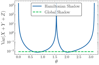
Figure 12: The variance performance of estimating $X+Y+Z$ using the Hamiltonian shadow with $H=\cos(\theta)Z+\sin(\theta)X$ and the original shadow. The measurement times is set to be $K=1000$ and the target state is a random pure state.

D.2 Multiqubit Hadamard Gates

In this section, we use another example to give the evidence that the performance of the Hamiltonian shadow is similar with the original shadow. The protocol is shown in Fig. 13, where the state $\rho$ evolves with a random diagonal unitary followed by a layer of Hadamard gates. Here $\rho$ can be regarded as the $\rho_{H}$ introduced in the previous section.

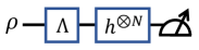
Figure 13: The Hamiltonian shadow with a random diagonal unitary followed by a layer of Hadamard gates.

Following the derivation in Sec. C, the shadow map for this setting is $\mathcal{M}(\rho)=\mathcal{N}(\rho)$, as the evolving unitary is $V_{H}\Lambda$ instead of $V_{H}\Lambda V_{H}^{\dagger}$. Using the matrix form of Hadamard gate, $h=\frac{1}{\sqrt{2}}\begin{bmatrix}1&1\\ 1&-1\end{bmatrix}$, every element of $X_{H}$ is

$$(X_{H})_{i,j}=\sum_{b}|\bra{i}h^{\otimes N}\ket{b}|^{2}\times|\bra{j}h^{\otimes N}\ket{b}|^{2}=2^{-N}.$$ (53)

Thus, the shadow map is

$$\mathcal{M}(\rho)=\sum_{i}\left(\sum_{j}(X_{H})_{i,j}\rho_{j,j}\right)\outerproduct{i}{i}+\sum_{i\neq j}X_{ij,ji}\rho_{j,i}\outerproduct{j}{i}=\frac{\mathbb{I}}{2^{N}}+\frac{1}{2^{N}}\sum_{i\neq j}\rho_{j,i}\outerproduct{j}{i}.$$ (54)

This Hamiltonian shadow map losses information of diagonal terms of $\rho$ and is thus not invertible. This can also be derived from the fact that the post-processing matrix $X_{H}$ is not invertible. At the same time, all off-diagonal terms of $X_{H}$ are nonzero. Therefore, $2^{N}\overline{\Lambda}h^{\otimes N}\outerproduct{b}{b}h^{\otimes N}\Lambda-\mathbb{I}$ gives the unbiased estimator of $\rho-\mathrm{diag}(\rho)$. This estimator can be used to estimate the expectation value of some observables with zero diagonal elements by $\hat{o}=2^{n}\Tr\left[\overline{\Lambda}h^{\otimes n}\outerproduct{b}{b}h^{\otimes n}\Lambda O\right]$. The variance of $\hat{o}$ is

$$\mathrm{Var}\left(\hat{o}\right)=2^{2N}\mathbb{E}_{\Lambda}\sum_{b}\Tr\left[\overline{\Lambda}h^{\otimes N}\outerproduct{b}{b}h^{\otimes N}\Lambda\rho\right]\Tr\left[\overline{\Lambda}h^{\otimes N}\outerproduct{b}{b}h^{\otimes N}\Lambda O\right]^{2}-\Tr(O\rho)^{2}=2^{2N}\begin{tabular}[]{c}\includegraphics[scale={0.25}]{figure/var_hadamard.pdf}\end{tabular}-\Tr(O\rho)^{2},$$ (55)

where $X_{3}=\sum_{b}h^{\otimes 3N}\outerproduct{bbb}{bbb}h^{\otimes 3N}$. To calculate the variance, we need to utilize the properties of $\Phi_{3}^{\mathrm{D}}(X_{3})$. As shown in Fig. 9, the third order integral has many terms. While, good thing is that, nonzero elements of all matrices are $2^{-2N}$. For example,

$$\left(\begin{tabular}[]{c}\includegraphics[scale={0.25}]{figure/var_Hadamard1.pdf}\end{tabular}\right)_{ijj,jij}=\sum_{b}\bra{ijj}h^{\otimes 3N}\ket{bbb}\bra{bbb}h^{\otimes 3N}\ket{jij}=\sum_{b}|\bra{i}h^{\otimes N}\ket{b}|^{2}|\bra{j}h^{\otimes N}\ket{b}|^{4}=2^{-2N}.$$ (56)

The proof for other terms are same. Therefore, with the indices contraction rule, the variance can be written as

$$\mathrm{Var}(\hat{o})=\sum_{i,j,k}\left(O_{i,i}O_{j,j}\rho_{k,k}+O_{i,i}O_{j,k}\rho_{k,j}+O_{i,k}O_{j,j}\rho_{k,i}+O_{i,j}O_{j,i}\rho_{k,k}+O_{i,j}O_{j,k}\rho_{k,i}+O_{i,k}O_{j,i}\rho_{k,j}\right)$$ (57)

$$- \sum_{i,j}\left(O_{i,i}O_{i,i}\rho_{j,j}+O_{i,j}O_{j,j}\rho_{j,i}+O_{i,i}O_{j,i}\rho_{i,j}+O_{i,j}O_{i,i}\rho_{j,i}+O_{i,i}O_{j,j}\rho_{j,j}+O_{i,j}O_{j,i}\rho_{i,i}+O_{i,i}O_{i,j}\rho_{j,i}+O_{i,j}O_{j,i}\rho_{j,j}+O_{i,i}O_{j,j}\rho_{i,i}\right)$$

$$+ 4\sum_{i}O_{i,i}O_{i,i}\rho_{i,i}-\Tr(O\rho)^{2}.$$

As $O$ has no diagonal terms, $O_{i,i}=0$, only a few terms in the above equation survives

$$\mathrm{Var}(\hat{o})= \sum_{i,j,k}\left(O_{i,j}O_{j,i}\rho_{k,k}+O_{i,j}O_{j,k}\rho_{k,i}+O_{i,k}O_{j,i}\rho_{k,j}\right)-\sum_{i,j}\left(O_{i,j}O_{j,i}\rho_{j,j}+O_{i,j}O_{j,i}\rho_{i,i}\right)-\Tr(O\rho)^{2}$$ (58)

$$\leq \Tr(O^{2})+2\Tr(O^{2}\rho)\leq 3\Tr(O^{2}),$$

where the first inequality holds as $O_{j,i}O_{i,j}\rho_{i,i}=|O_{j,i}|^{2}\rho_{i,i}\geq 0$. Notice that $\Tr(O^{2})+2\Tr(O^{2}\rho)$ is exactly the upper bound for original shadow when using global Clifford unitaries [36]. This result shows a strong evidence that the random diagonal shadow can have a similar performance with the original shadow protocol. Besides, the inability to estimate diagonal information of $\rho$ is not a big problem in practice, as we can directly perform computational basis measurements on $\rho$ to extract these information. The final thing we want to emphasis is that, similar with the original shadow protocol, the leading term of variance is also

$$\sum_{i,j,k}(X_{3})_{ijk,jik}O_{i,j}O_{j,i}\rho_{k,k}=\begin{tabular}[]{c}\includegraphics[scale={0.25}]{figure/var_Hadamard2.pdf}\end{tabular},$$ (59)

which also introduces the indices contraction between two observable matrices.

We also numerically show that the performance of Hadamard-based shadow is similar to the global shadow. In Fig. 14, we adopt the original shadow with global Clifford gates and the Hadamard-based Hamiltonian shadow to estimate the Pauli observable $X^{\otimes N}$, which has no diagonal elements and satisfies the requirement of detecting with Hadamard shadow. It is shown that the variance scaling of these two protocols are highly similar.

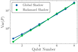
Figure 14: The comparison between the global shadow and Hadamard-based Hamiltonian shadow in estimating the expectation value of $P=X^{\otimes N}$. We set $K=10$ and the target state to be a random pure state.

Appendix E Variance Analysis

In this section, we provide a systematic analysis of the variance of Hamiltonian shadow and use some approximation to simplify its expression. We also start from global version of Hamiltonian shadow, shown in Fig. 10(a), and generalize the result to local one, shown in Fig. 10(b).

Given the target observable $O$, the shadow estimator is

$$\hat{o}=\Tr\left[OV_{H}\mathcal{N}^{-1}(\overline{\Lambda}_{t}V_{H}^{\dagger}\outerproduct{b}{b}V_{H}\Lambda_{t})V_{H}^{\dagger}\right]=\Tr\left[(\mathcal{N}^{-1})^{\dagger}(V_{H}^{\dagger}OV_{H})\overline{\Lambda}_{t}V_{H}^{\dagger}\outerproduct{b}{b}V_{H}\Lambda_{t}\right].$$ (60)

With the definition of $\mathcal{N}^{-1}$, we have

$$\Tr[A\mathcal{N}^{-1}(B)]=\sum_{i,j}A_{i,i}(X_{H}^{-1})_{i,j}B_{j,j}+\sum_{i\neq j}(X_{H})_{i,j}^{-1}B_{i,j}A_{j,i}=\sum_{i,j}B_{i,i}(X_{H}^{-1})_{i,j}A_{j,j}+\sum_{i\neq j}(X_{H})_{i,j}^{-1}A_{i,j}B_{j,i}=\Tr[\mathcal{N}^{-1}(A)B]$$ (61)

for two square matrices $A$ and $B$, where the second equality holds as $X_{H}$ is a real symmetric matrix. This equation shows that $(\mathcal{N}^{-1})^{\dagger}=\mathcal{N}^{-1}$. Combining this property and Eq. (60), the variance can be written as

$$\mathrm{Var}(\hat{o}) =\mathbb{E}_{b,t}\hat{o}^{2}-\Tr(O\rho)^{2}$$ (62)

$$=\mathbb{E}_{t}\sum_{b}\bra{b}e^{-iHt}\rho e^{iHt}\ket{b}\hat{o}^{2}-\Tr(O\rho)^{2}$$

$$=\mathbb{E}_{t}\sum_{b}\Tr\left\{\left[\mathcal{N}^{-1}(V_{H}^{\dagger}OV_{H})^{\otimes 2}\otimes V_{H}^{\dagger}\rho V_{H}\right]\left[\left(\overline{\Lambda}_{t}V_{H}^{\dagger}\right)^{\otimes 3}\outerproduct{bbb}{bbb}\left(V_{H}\Lambda_{t}\right)^{\otimes 3}\right]\right\}-\Tr(O\rho)^{2}.$$

Define $X_{3}=\sum_{b}\left(V_{H}^{\dagger}\outerproduct{b}{b}V_{H}\right)^{\otimes 3}$, the leading term of variance can be graphically represented as

$$\mathbb{E}_{b,t}\hat{o}^{2} =\mathbb{E}_{t}\left(\sum_{b}\begin{tabular}[]{c}\includegraphics[scale={0.25}]{figure/var_derivation1.pdf}\end{tabular}\right)=\begin{tabular}[]{c}\includegraphics[scale={0.25}]{figure/var_derivation2.pdf}\end{tabular}$$ (63)

$$=\Tr\left\{\left[\mathcal{N}^{-1}(V_{H}^{\dagger}OV_{H})^{\otimes 2}\otimes V_{H}^{\dagger}\rho V_{H}\right]\Phi_{3}^{\mathrm{D}}(X_{3})\right\},$$

where grey dashed lines represent the trace function. In addition to the observable and state, the variance of random diagonal shadow highly depends on the diagonal unitary $V_{H}$. As discussed in Appendix D.1, when $V_{H}$ approaches the identity matrix, it is easy for the Hamiltonian shadow to extract information of diagonal elements of $V_{H}^{\dagger}\rho V_{H}$ while hard for off-diagonal elements. And as shown in Appendix D.2, when $V_{H}$ approaches the tensor product of Hadamard gates, it is hard to extract information of diagonal terms of $V_{H}^{\dagger}\rho V_{H}$.

Similar with the original shadow protocol, the variance of the Hamiltonian shadow protocol does not necessitate that $\Lambda_{t}$ be a perfect random diagonal unitary; a diagonal unitary three-design is sufficient. This is because that in the derivation of the variance, we only require the use of $\Phi_{3}^{\mathrm{D}}(\cdot)$. Another consequence of the third-order integral is that, although the third-order degeneracy of Hamiltonian does not affect the unbiasedness of Hamiltonian shadow, it does affect the variance of it.

An important property of Hamiltonian shadow variance is that $\mathbb{E}_{b,t}\hat{o}^{2}=1$ when $O=\mathbb{I}$. This property can be easily derived from the fact that $\mathcal{N}$ and $\mathcal{N}^{-1}$ are both trace-preserving. We give another proof for this property. Given $O=\mathbb{I}$, the estimator can be written as

$$\hat{o}= \Tr\left[\mathcal{N}^{-1}(V_{H}^{\dagger}\mathbb{I}V_{H})\overline{\Lambda}_{t}V_{H}^{\dagger}\outerproduct{b}{b}V_{H}\Lambda_{t}\right]=\bra{b}V_{H}\mathcal{N}^{-1}(\mathbb{I})V_{H}^{\dagger}\ket{b}$$ (64)

$$= \sum_{i}\sum_{j}(X_{H}^{-1})_{ij}\bra{b}V_{H}\outerproduct{i}{i}V_{H}^{\dagger}\ket{b}$$

$$= \sum_{i}\sum_{j}\left[(V_{H}^{\mathrm{sq}})^{-1}((V_{H}^{\mathrm{sq}})^{T})^{-1}\right]_{i,j}(V_{H}^{\mathrm{sq}})_{b,i}$$

$$= \sum_{j}(V_{H}^{\mathrm{sq}})^{-1}_{j,b},$$

where we adopt the definition of $\mathcal{N}^{-1}$ and $X_{H}=(V_{H}^{\mathrm{sq}})^{T}V_{H}^{\mathrm{sq}}$. As $(V_{H}^{\mathrm{sq}})^{-1}V_{H}^{\mathrm{sq}}=\mathbb{I}$, we have

$$\sum_{j}(V_{H}^{\mathrm{sq}})^{-1}_{j,b}=\sum_{j}(V_{H}^{\mathrm{sq}})^{-1}_{j,b}\sum_{b}(V_{H}^{\mathrm{sq}})_{b,i}=\sum_{j}\left(\sum_{b}(V_{H}^{\mathrm{sq}})^{-1}_{j,b}(V_{H}^{\mathrm{sq}})_{b,i}\right)=\sum_{j}(\delta_{i,j})=1,$$ (65)

where we use the property of unitary matrix that $\sum_{b}(V_{H}^{\mathrm{sq}})_{b,i}=1$. From above derivations, we know that, when setting $O=\mathbb{I}$, the estimator and $\mathbb{E}_{t,b}\hat{o}^{2}$ are always $1$, no matter of the measurement result $b$. Thus, the corresponding variance is zero. This is an important property for local version of Hamiltonian shadow. Suppose we use the evolution of $\bigotimes_{p=1}^{N}e^{-iH_{p}t}$ to perform Hamiltonian shadow on $\rho$, shown in Fig. 10, the variance of estimating $O=\bigotimes_{p=1}^{N}O_{p}$ can be easily generalized from the result of global version Hamiltonian shadow,

$$\mathbb{E}_{b,t}\hat{o}^{2}=\prod_{p=1}^{N}\mathbb{E}_{t,b_{p}}\hat{o}_{p}^{2}.$$ (66)

Using the property of $\mathbb{E}_{b,t}\hat{o}^{2}=1$ for $O=\mathbb{I}$, the variance of estimating some local observable does not depend on the total qubit number of $\rho$, but only the locality of $O$.

E.1 Hamiltonian Shadow Norm

To benefit our description of the sample complexity of Hamiltonian shadow, we define the Hamiltonian shadow norm of an observable as

$$\norm{O}_{\mathrm{HShadow}}=\max_{\sigma}\left(\mathbb{E}_{t}\sum_{b}\bra{b}e^{-iHt}\sigma e^{iHt}\ket{b}\hat{o}^{2}\right)^{1/2}= \max_{\sigma}\left(\mathbb{E}_{t}\sum_{b}\bra{b}e^{-iHt}\sigma e^{iHt}\ket{b}\bra{b}V_{H}\Lambda_{t}\mathcal{N}^{-1}(V_{H}^{\dagger}OV_{H})\overline{\Lambda}_{t}V_{H}^{\dagger}\ket{b}^{2}\right)^{1/2}$$ (67)

$$= \max_{\sigma}\left(\begin{tabular}[]{c}\includegraphics[scale={0.25}]{figure/var_derivation4.pdf}\end{tabular}\right)^{1/2}.$$

It is easy to prove that the Hamiltonian shadow norm is non-negative and homogeneous, $\norm{0}_{\mathrm{HShadow}}=0$. We need to prove the triangle inequality of Hamiltonian shadow norm. Denoting $x_{b}=\bra{b}e^{-iHt}\sigma e^{iHt}\ket{b}^{1/2}\bra{b}V_{H}\Lambda_{t}\mathcal{N}^{-1}(V_{H}^{\dagger}O_{1}V_{H})\overline{\Lambda}_{t}V_{H}^{\dagger}\ket{b}$, and $y_{b}=\bra{b}e^{-iHt}\sigma e^{iHt}\ket{b}^{1/2}\bra{b}V_{H}\Lambda_{t}\mathcal{N}^{-1}(V_{H}^{\dagger}O_{2}V_{H})\overline{\Lambda}_{t}V_{H}^{\dagger}\ket{b}$, the Hamiltonian shadow norm of $O_{1}+O_{2}$ is thus

$$\norm{O_{1}+O_{2}}_{\mathrm{HShadow}}=\max_{\sigma}\left(\mathbb{E}_{t}\sum_{b}(x_{b}+y_{b})^{2}\right)^{1/2}.$$ (68)

According to the triangle inequality of coordinate norm, we have

$$\left(\sum_{b}(x_{b}+y_{b})^{2}\right)^{1/2}=\absolutevalue{\vec{x}+\vec{y}}\leq\absolutevalue{\vec{x}}+\absolutevalue{\vec{y}}=\left(\sum_{b}x_{b}^{2}\right)^{1/2}+\left(\sum_{b}y_{b}^{2}\right)^{1/2}.$$ (69)

According to the property of root function, one can easily prove that $\left(\mathbb{E}_{t}\sum_{b}(x_{b}+y_{b})^{2}\right)^{1/2}\leq\left(\mathbb{E}_{t}\sum_{b}x_{b}^{2}\right)^{1/2}+\left(\mathbb{E}_{t}\sum_{b}y_{b}^{2}\right)^{1/2}$. Therefore,

$$\norm{O_{1}+O_{2}}_{\mathrm{HShadow}}\leq \max_{\sigma}\left[\left(\mathbb{E}_{t}\sum_{b}x_{b}^{2}\right)^{1/2}+\left(\mathbb{E}_{t}\sum_{b}y_{b}^{2}\right)^{1/2}\right]$$ (70)

$$\leq \max_{\sigma}\left(\mathbb{E}_{t}\sum_{b}x_{b}^{2}\right)^{1/2}+\max_{\sigma}\left(\mathbb{E}_{t}\sum_{b}x_{b}^{2}\right)^{1/2}$$

$$= \norm{O_{1}}_{\mathrm{HShadow}}+\norm{O_{2}}_{\mathrm{HShadow}},$$

which concludes the triangle inequality.

According to Eq. (62), when estimating $\tr(O\rho)$ with Hamiltonian shadow, the variance is upper bounded by $\norm{O}_{\mathrm{HShadow}}^{2}$. Therefore, adopting the median-of-mean data processing method [36], we can bound the sample complexity $K$ of estimating $M$ observables using the Hamiltonian shadow norm

$$K=\mathcal{O}\left(\mathrm{log}(M)\frac{\max_{i}\norm{O_{i}}_{\mathrm{HShadow}}^{2}}{\epsilon^{2}}\right),$$ (71)

where $\epsilon$ is the additive error.

E.2 Variance Approximation

It is hard to derive a simple expression for the variance of Hamiltonian shadow. While, we can use some reasonable approximations to give a function that can largely reflect the scaling of variance. According to derivations of original shadow protocol and the Hadamard-based diagonal shadow, we can reasonably assume that the leading term of Hamiltonian shadow variance is

$$\begin{tabular}[]{c}\includegraphics[scale={0.25}]{figure/var_derivation3.pdf}\end{tabular}=\Tr\left\{\left(\mathcal{N}^{-1}\otimes\mathcal{N}^{-1}\otimes\mathcal{I}\right)\left[\sum_{i,j,k}(X_{3})_{ijk,jik}\outerproduct{ijk}{jik}\right]\left[(V_{H}^{\dagger}OV_{H})^{\otimes 2}\otimes V_{H}^{\dagger}\rho V_{H}\right]\right\},$$ (72)

where $\mathcal{I}$ represents the identity map. This term is the leading term because it introduces the indices contraction between two observables $O$ while traces over the density matrix $\rho$. Similar terms in variances of the original shadow protocol and the Hadamard diagonal shadow protocol give the term of $\Tr(O^{2})$, which is the leading term of those two variances. Now, we will try to simplify this term.

We first divide this term into two parts

$$\Tr\left\{\left(\mathcal{N}^{-1}\otimes\mathcal{N}^{-1}\otimes\mathcal{I}\right)\left[\sum_{i,j,k}(X_{3})_{ijk,jik}\outerproduct{ijk}{jik}\right]\left[(V_{H}^{\dagger}OV_{H})^{\otimes 2}\otimes V_{H}^{\dagger}\rho V_{H}\right]\right\}$$ (73)

$$= \sum_{i\neq j}\sum_{k}(X_{3})_{ijk,jik}\Tr\left[\mathcal{N}^{-1}\left(\outerproduct{i}{j}\right)V_{H}^{\dagger}OV_{H}\right]\Tr\left[\mathcal{N}^{-1}\left(\outerproduct{j}{i}\right)V_{H}^{\dagger}OV_{H}\right]\bra{k}V_{H}^{\dagger}\rho V_{H}\ket{k}$$

$$+ \sum_{i}\sum_{k}(X_{3})_{iik,iik}\Tr\left[\mathcal{N}^{-1}(\outerproduct{i}{i})V_{H}^{\dagger}OV_{H}\right]^{2}\bra{k}V_{H}^{\dagger}\rho V_{H}\ket{k}.$$

The first part contains exponentially more terms and is generally exponentially larger than the second part. Thus, we only focus on the first part and expand it. By definition, the element of $X_{3}$ is

$$(X_{3})_{ijk,jik}=\sum_{b}\bra{ijk}(V_{H}^{\dagger})^{\otimes 3}\outerproduct{bbb}{bbb}V_{H}^{\otimes 3}\ket{jik}=\sum_{b}|(V_{H})_{b,i}|^{2}|(V_{H})_{b,j}|^{2}|(V_{H})_{b,k}|^{2}.$$ (74)

Substituting it into the Eq. (73), we find the first part to be

$$\sum_{i\neq j}\sum_{k}\sum_{b}|(V_{H})_{b,i}|^{2}|(V_{H})_{b,j}|^{2}|(V_{H})_{b,k}|^{2}(X_{H})_{i,j}^{-2}\bra{j}V_{H}^{\dagger}OV_{H}\ket{i}\bra{i}V_{H}^{\dagger}OV_{H}\ket{j}\bra{k}V_{H}^{\dagger}\rho V_{H}\ket{k}$$ (75)

$$= \sum_{i\neq j}\sum_{b}|(V_{H})_{b,i}|^{2}|(V_{H})_{b,j}|^{2}(X_{H})_{i,j}^{-2}\bra{j}V_{H}^{\dagger}OV_{H}\ket{i}\bra{i}V_{H}^{\dagger}OV_{H}\ket{j}\sum_{k}|(V_{H})_{b,k}|^{2}\bra{k}V_{H}^{\dagger}\rho V_{H}\ket{k}.$$

Here, $\bra{k}V_{H}^{\dagger}\rho V_{H}\ket{k}$ is the diagonal term of $V_{H}^{\dagger}\rho V_{H}$ and $\rho$ is the target quantum state which normally has no relationship with $V_{H}$. Thus, it is reasonable to assume $\bra{k}V_{H}^{\dagger}\rho V_{H}\ket{k}\approx\frac{1}{d}$ for all $k$. With this approximation, we have $\sum_{k}|(V_{H})_{b,k}|^{2}\bra{k}V_{H}^{\dagger}\rho V_{H}\ket{k}=\frac{1}{d}$. Then, the first part becomes

$$\sum_{i\neq j}\sum_{b}|(V_{H})_{b,i}|^{2}|(V_{H})_{b,j}|^{2}(X_{H})_{i,j}^{-2}\bra{j}V_{H}^{\dagger}OV_{H}\ket{i}\bra{i}V_{H}^{\dagger}OV_{H}\ket{j}\sum_{k}|(V_{H})_{b,k}|^{2}\bra{k}V_{H}^{\dagger}\rho V_{H}\ket{k}$$ (76)

$$\approx \frac{1}{d}\sum_{i\neq j}\sum_{b}|(V_{H})_{b,i}|^{2}|(V_{H})_{b,j}|^{2}(X_{H})_{i,j}^{-2}\bra{j}V_{H}^{\dagger}OV_{H}\ket{i}\bra{i}V_{H}^{\dagger}OV_{H}\ket{j}$$

$$= \frac{1}{d}\sum_{i\neq j}(X_{H})_{i,j}(X_{H})_{i,j}^{-2}\bra{j}V_{H}^{\dagger}OV_{H}\ket{i}\bra{i}V_{H}^{\dagger}OV_{H}\ket{j}$$

$$= \frac{1}{d}\sum_{i\neq j}(X_{H})_{i,j}^{-1}|\bra{i}V_{H}^{\dagger}OV_{H}\ket{j}|^{2},$$

which is the function of $f(O,V_{H})$ we introduced in the main context.

E.3 Nonlinear Observables

It is straightforward to use the Hamiltonian shadow to estimate nonlinear quantities, like $\Tr(O\rho^{\otimes 2})$. After $K$ times of experiments, we get a total of $K$ unbiased estimators of $\rho$, labeled as $\{\hat{\rho}_{i}\}_{i=1}^{K}$. Using these estimators, we can construct the unbiased estimator of $\Tr(O\rho^{\otimes 2})$ as

$$\hat{o}_{2}=\frac{1}{K(K-1)}\sum_{i\neq j}\Tr\left[O\left(\hat{\rho}_{i}\otimes\hat{\rho}_{j}\right)\right].$$ (77)

The variance is

$$\mathrm{Var}(\hat{o}_{2})=\frac{1}{K(K-1)}\mathrm{Var}\left(\Tr\left[O\left(\hat{\rho}\otimes\hat{\rho}^{\prime}\right)\right]\right)=\frac{1}{K(K-1)}\left\{\mathbb{E}\Tr\left[O\left(\hat{\rho}\otimes\hat{\rho}^{\prime}\right)\right]^{2}-\Tr(O\rho^{\otimes 2})^{2}\right\},$$ (78)

where $\hat{\rho}$ and $\hat{\rho}^{\prime}$ represent two independent estimators constructed using Hamiltonian shadow.

When $O=S$, $\tr(O\rho^{\otimes 2})$ gives the value of purity, $\tr(\rho^{2})$, which is important for our numerical demonstration in main context. So, we start from $O=S$ and derive the approximate variance of it, which can be easily extended to general nonlinear observables. Substituting the form of Hamiltonian shadow estimator, we have

$$\mathbb{E}\Tr\left[S\left(\hat{\rho}\otimes\hat{\rho}^{\prime}\right)\right]^{2}=\mathbb{E}_{t,t^{\prime}}\sum_{b,b^{\prime}}\bra{b}V_{H}\Lambda_{t}V_{H}^{\dagger}\rho V_{H}\overline{\Lambda}_{t}V_{H}^{\dagger}\ket{b}\bra{b^{\prime}}V_{H}\Lambda_{t^{\prime}}V_{H}^{\dagger}\rho V_{H}\overline{\Lambda}_{t^{\prime}}V_{H}^{\dagger}\ket{b^{\prime}}\Tr\left[S\left(\hat{\rho}\otimes\hat{\rho}^{\prime}\right)\right]^{2},$$ (79)

which can be calculated in a graphical way

$$\mathbb{E}\Tr\left[S\left(\hat{\rho}\otimes\hat{\rho}^{\prime}\right)\right]^{2}= \mathbb{E}_{t,t^{\prime}}\left[\sum_{b,b^{\prime}}\begin{tabular}[]{c}\includegraphics[scale={0.25}]{figure/nonlinear_variance.pdf}\end{tabular}\right]=\begin{tabular}[]{c}\includegraphics[scale={0.25}]{figure/nonlinear_variance1.pdf}\end{tabular}$$ (80)

$$= \Tr\left\{\Tr_{3}\left\{\mathcal{N}^{-1}\otimes\mathcal{N}^{-1}\otimes\mathcal{I}\left[\Phi_{3}^{\mathrm{D}}(X_{3})\right]\left(\mathbb{I}^{\otimes 2}\otimes V_{H}^{\dagger}\rho V_{H}\right)\right\}^{2}\right\}.$$

Adopting the same approximation for linear observables, the matrix $\Tr_{3}\left\{\mathcal{N}^{-1}\otimes\mathcal{N}^{-1}\otimes\mathcal{I}\left[\Phi_{3}^{\mathrm{D}}(X_{3})\right]\left(\mathbb{I}^{\otimes 2}\otimes V_{H}^{\dagger}\rho V_{H}\right)\right\}$ can be approximated by $\frac{1}{d}\sum_{i\neq j}\frac{1}{(X_{H})_{i,j}}\outerproduct{ij}{ji}$. Substituting this approximation, we have

$$\mathbb{E}\Tr\left[S\left(\hat{\rho}\otimes\hat{\rho}^{\prime}\right)\right]^{2}\sim \begin{tabular}[]{c}\includegraphics[scale={0.25}]{figure/nonlinear_variance2.pdf}\end{tabular}$$ (81)

$$= \frac{1}{d^{2}}\sum_{i\neq j}\sum_{i^{\prime}\neq j^{\prime}}\frac{1}{(X_{H})_{i,j}(X_{H})_{i^{\prime},j^{\prime}}}\Tr(S\outerproduct{ii^{\prime}}{jj^{\prime}})\Tr(S\outerproduct{jj^{\prime}}{ii^{\prime}})$$

$$= \frac{1}{d^{2}}\sum_{i\neq j}\frac{1}{(X_{H})_{i,j}^{2}}.$$

For a general nonlinear observable $O$, the exact and approximate variances can be derived in a similar way,

$$\mathbb{E}\Tr\left[O\left(\hat{\rho}\otimes\hat{\rho}^{\prime}\right)\right]^{2}= \Tr\left\{V_{H}^{\dagger\otimes 4}\left(S_{23}O^{\otimes 2}S_{23}\right)V_{H}^{\otimes 4}\Tr_{3}\left\{\mathcal{N}^{-1}\otimes\mathcal{N}^{-1}\otimes\mathcal{I}\left[\Phi_{3}^{\mathrm{D}}(X_{3})\right]\left(\mathbb{I}^{\otimes 2}\otimes V_{H}^{\dagger}\rho V_{H}\right)\right\}^{\otimes 2}\right\}$$ (82)

$$\sim \frac{1}{d^{2}}\sum_{i\neq j}\sum_{i^{\prime}\neq j^{\prime}}\frac{1}{(X_{H})_{i,j}(X_{H})_{i^{\prime},j^{\prime}}}\absolutevalue{\bra{jj^{\prime}}(V_{H}^{\dagger})^{\otimes 2}OV_{H}^{\otimes 2}\ket{ii^{\prime}}}^{2},$$

where $S_{23}$ is the swap operator acting on the second party of the first $O$ and the first party of the second $O$.

We also use the numerical experiment to show the accuracy of our approximation, as shown in Fig. 15. Besides, it is also shown that the performance of Hamiltonian shadow can approach the global shadow with a proper Hamiltonian, even in predicting nonlinear observables.

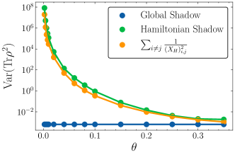
Figure 15: The scaling of variance for estimating state purity. Similar with the setting in main context, we set $V_{H}=e^{iP\theta}$, where $P$ is a random Hermitian matrix and $\theta$ quantifies the difference between $V_{H}$ and a diagonal unitary. The value of every point is chosen by taking the median of ten independently sampled $P$. The target state is set to be a four-qubit GHZ state and the experiment times is set to be $K=1000$.

Appendix F Detection Capability

After systematically demonstrating the effectiveness of Hamiltonian shadow protocol and its performances, we now discuss several scenarios where the Hamiltonian shadow protocol does not work. In Appendix C, we have shown how to determine Choi matrices of Hamiltonian shadow map in different scenarios, including those involving limited evolution time and existence of degeneracy. In principle, we can directly employ these Choi matrices and mathematically determine if they correspond to invertible maps. In this section, we analyze the reversibility of Hamiltonian shadow map from the perspective of state learning instead of linear algebra. These analysis not only help us to choose appropriate Hamiltonians for Hamiltonian shadow, but also deepen our understanding for Hamiltonian shadow protocol. We discuss four main factors that affect the reversibility of Hamiltonian shadow map, the eigenvalues and eigenstates of Hamiltonian $H$, the incomplete measurement, and the target state.

F.1 Eigenvalues

Degeneracy is the first property of real-world Hamiltonian that would affect the reversibility of Hamiltonian shadow map, which makes several eigenvalues of $e^{-iHt}$ correlated. We have introduced the integral rule of random diagonal unitary with degeneracy by Eq. (17) and Eq. (19). In these scenarios, even with infinite time scale $\Delta t$, the shadow map $\mathcal{M}_{H}$, or equivalently, $\mathcal{N}$, will deviate from the case of ideal random diagonal unitaries, as $\Phi_{2}^{\Delta t}(X_{2})\neq\Phi_{2}^{\mathrm{D}}(X_{2})$ for $\Delta t\to\infty$. This not only changes the Choi matrix of Hamiltonian shadow map, but may even make it irreversible. Based on the logic of state learning, we can formally prove that:

Proposition 2.

If $H$ has at least two same eigenvalues, the Hamiltonian shadow protocol is not tomography-complete.

Proof.

Without loss of generality, we assume $e^{-iHt}=V_{H}\Lambda_{t}V_{H}^{\dagger}$ with two same eigenvalues $\Lambda_{a_{1},a_{1}}=\Lambda_{a_{2},a_{2}}$. As $V_{H}$ is a fixed unitary, completely learning $\rho$ is equivalent with completely learning $\rho_{H}=V_{H}^{\dagger}\rho V_{H}$. As the estimating probability $\bra{b}e^{-iHt}\rho e^{iHt}\ket{b}=\bra{b}V_{H}\Lambda_{t}\rho_{H}\overline{\Lambda}_{t}V_{H}^{\dagger}\ket{b}$, we need to decide whether measurements in basis of $\{\overline{\Lambda}_{t}V_{H}^{\dagger}\outerproduct{b}{b}V_{H}\Lambda_{t}\}_{t,b}$ can extract full information of a state. Assuming $\Lambda_{t}=\mathrm{diag}(e^{-iE_{1}t},\cdots,e^{-iE_{d}t})$, the matrix form of $\Lambda_{t}\rho_{H}\overline{\Lambda}_{t}$ is

$$\Lambda_{t}\rho_{H}\overline{\Lambda}_{t}=\sum_{j,k}(\rho_{H})_{j,k}e^{-i(E_{j}-E_{k})t}\outerproduct{j}{k}.$$ (83)

With the condition of $\Lambda_{a_{1},a_{1}}=\Lambda_{a_{2},a_{2}}$, in addition to the diagonal terms, $(\Lambda_{t}\rho_{H}\overline{\Lambda}_{t})_{a_{1},a_{2}}$ and $(\Lambda_{t}\rho_{H}\overline{\Lambda}_{t})_{a_{2},a_{1}}$ are also independent with the evolution time $t$. As $V_{H}$ is a fixed unitary, the probability $\bra{b}V_{H}\Lambda_{t}\rho_{H}\overline{\Lambda}_{t}V_{H}^{\dagger}\ket{b}$ is a linear function of all elements of $\rho_{H}$. While, coefficients of diagonal terms of $\rho_{H}$, $(\rho_{H})_{a_{1},a_{2}}$, and $(\rho_{H})_{a_{2},a_{1}}$ are independent with $t$. Thus, varying evolution time will not provide more independent equations to determine these terms. Using $d$ independent equations to estimate a total of $d+2$ unknown parameters is prohibited, so one cannot learn $\rho$ completely and the Hamiltonian shadow protocol is not tomography-complete.

∎

Notice that, even with degeneracy, other elements of $\Lambda_{t}\rho_{H}\overline{\Lambda}_{t}$ that depends on $t$ can still be estimated. This is because one could measure in many different evolution time $t$ and acquire many independent equations to determine these elements. Thus, although the Hamiltonian shadow protocol is not tomography-complete in this case, we can still estimate certain observables with special forms. Besides, if more than one degenerate Hamiltonians with different $V_{H}$ are accessible, it is possible to recover the tomography-completeness of the Hamiltonian shadow.

We can also use the proof to understand why a Hamiltonian without any degeneracy can be used to completely learn a state. In this scenario, all off-diagonal terms of $\Lambda_{t}\rho_{H}\overline{\Lambda}_{t}$ depend on evolution time $t$ with different coefficients. Subsequently, the diagonal elements of $V_{H}\Lambda_{t}\rho_{H}\overline{\Lambda}_{t}V_{H}^{\dagger}$ linearly depend on these off-diagonal terms with different time-dependent coefficients. Thus, one could estimate all these off-diagonal terms by measuring $V_{H}\Lambda_{t}\rho_{H}\overline{\Lambda}_{t}V_{H}^{\dagger}$ in computational basis for different evolution time, as these measurements provide sufficiently many independent equations to determine these terms. At the same time, the number of time-independent diagonal terms of $\Lambda_{t}\rho_{H}\overline{\Lambda}_{t}$ is no more than the number of measurement results. As a result, all elements of $\rho_{H}$ can be estimated and the Hamiltonian shadow protocol is tomography-complete.

As introduced previously, the specific form of Hamiltonian shadow map is based on the second-order integral of random diagonal unitaries. As shown in Eq. (19), the second-order degeneracy can also affect the second-order integral, and therefore change the Choi matrix of Hamiltonian shadow map and make the $X_{H}$ matrix cannot fully describe $\mathcal{N}$. Thus, a natural question is, does the second-order degeneracy affect the reversibility of the shadow map? We prove that this is not the case:

Proposition 3.

Given a non-degenerate Hamiltonian with second order degeneracy, the corresponding Hamiltonian shadow protocol is tomography-complete. Here by second-order degeneracy, we mean that some eigen-energies of $H$ satisfy $E_{a_{1}}+E_{a_{2}}=E_{b_{1}}+E_{b_{2}}$ with $a_{1}\neq b_{1}$, $a_{1}\neq b_{2}$, $a_{2}\neq b_{1}$, $a_{2}\neq b_{2}$, and $a_{1}\neq a_{2}$.

Proof.

With second-order degeneracy, the evolved state in this situation is

$$\Lambda_{t}\rho_{H}\overline{\Lambda}_{t}= \sum_{j,k}(\rho_{H})_{j,k}e^{-i(E_{j}-E_{k})t}\outerproduct{j}{k}$$ (84)

$$= \cdots+\left[(\rho_{H})_{a_{1},b_{1}}e^{-i(E_{a_{1}}-E_{b_{1}})t}\outerproduct{a_{1}}{b_{1}}+(\rho_{H})_{b_{2},a_{2}}e^{-i(E_{b_{2}}-E_{a_{2}})t}\outerproduct{b_{2}}{a_{2}}+h.c\right]$$

$$= \cdots+\left\{e^{-i(E_{a_{1}}-E_{b_{1}})t}\left[(\rho_{H})_{a_{1},b_{1}}\outerproduct{a_{1}}{b_{1}}+(\rho_{H})_{b_{2},a_{2}}\outerproduct{b_{2}}{a_{2}}\right]+h.c\right\},$$

where we use the condition that $E_{a_{1}}-E_{b_{1}}=E_{b_{2}}-E_{a_{2}}$. Thus, coefficients of $(\rho_{H})_{a_{1},b_{1}}$ and $(\rho_{H})_{b_{2},a_{2}}$ are always same at any evolution time $t$. This also holds true for coefficients of $(\rho_{H})_{a_{1},b_{2}}$ and $(\rho_{H})_{b_{1},a_{2}}$. Similar to the case of non-degenerate Hamiltonian, in the current setting, other off-diagonal elements except for $(\rho_{H})_{a_{1},b_{1}}$, $(\rho_{H})_{b2,a2}$, $(\rho_{H})_{a_{1},b_{2}}$, and $(\rho_{H})_{b_{1},a_{2}}$ and all diagonal elements of $\Lambda_{t}\rho_{H}\overline{\Lambda}_{t}$ can still be estimated. We will prove that these four elements can also be estimated.

We first consider the estimation of $(\rho_{H})_{a_{1},b_{1}}$ and $(\rho_{H})_{b_{2},a_{2}}$. Assuming $(\rho_{H})_{a_{1},b_{1}}=r_{1}+is_{1}$ and $(\rho_{H})_{a_{2},b_{2}}=r_{2}+is_{2}$, the diagonal element of $V_{H}\Lambda_{t}\rho_{H}\overline{\Lambda}_{t}V_{H}^{\dagger}$ can be written as

$$\bra{j}V_{H}\Lambda_{t}\rho_{H}\overline{\Lambda}_{t}V_{H}^{\dagger}\ket{j}=\cdots+\cos\left[(E_{a_{1}}-E_{b_{1}})t\right]\left(\alpha^{j}_{1}r_{1}+\alpha^{j}_{2}r_{2}+\alpha^{j}_{3}s_{1}+\alpha^{j}_{4}s_{2}\right)+\sin\left[(E_{a_{1}}-E_{b_{1}})t\right]\left(\beta^{j}_{1}r_{1}+\beta^{j}_{2}r_{2}+\beta^{j}_{3}r_{3}+\beta^{j}_{4}r_{4}\right),$$ (85)

where $\alpha$ and $\beta$ are coefficients determined solely by $V_{H}$. So, by collecting measurement results $\bra{j}V_{H}\Lambda_{t}\rho_{H}\overline{\Lambda}_{t}V_{H}^{\dagger}\ket{j}$ with different time $t$ and $\ket{j}$ can help us to estimate values of $\left(\alpha^{j}_{1}r_{1}+\alpha^{j}_{2}r_{2}+\alpha^{j}_{3}s_{1}+\alpha^{j}_{4}s_{2}\right)$ and $\left(\beta^{j}_{1}r_{1}+\beta^{j}_{2}r_{2}+\beta^{j}_{3}r_{3}+\beta^{j}_{4}r_{4}\right)$ for many different $\alpha$ and $\beta$. Solving these equations helps to get values of $r_{1}$, $r_{2}$, $s_{1}$, and $s_{2}$. Following the same logic, $(\rho_{H})_{a_{1},b_{2}}$, and $(\rho_{H})_{b_{1},a_{2}}$ can also be estimated. Thus, the Hamiltonian shadow is still tomography-complete. ∎

Denote $R(\mathcal{C})$ to be a matrix constructed by permuting indices of Choi matrix, $[R(\mathcal{C})]_{ij,kl}=\mathcal{C}_{lj,ik}$. According to the concatenating rule of Choi matrices, if $R(\mathcal{C})$ is an invertible matrix, the corresponding map is invertible, and vise versa. We numerically substantiated Proposition 2 and Proposition 3 by constructing Choi matrices of Hamiltonian shadow maps using Eq. (17) and Eq. (19) and the matrix $R(\mathcal{C})$. We verified that the matrix $R(\mathcal{C})$ is irreversible for first-order degeneracy, while invertible for second-order case.

Our analysis is based on the most fundamental perspective, the state learning task, which can also be used to understand why single-patch Hamiltonians used in local Hamiltonian shadow protocol, Fig. 10(b), need to be independent. If the evolution unitary is $U=\bigotimes_{p=1}^{N}e^{-iH_{p}t}$, the corresponding Hamiltonian is $H=\sum_{p=1}^{N}H_{p}\otimes\mathbb{I}_{[N]-p}$, where $H_{p}$ only acts on patch $p$ and $\mathbb{I}_{[N]-p}$ is the identity operator acting on other patches. If two Hamiltonians are same, $H_{p}=H_{p^{\prime}}$, $H$ will be a degenerate Hamiltonian. According to Proposition 2, such Hamiltonian cannot be used to completely learn a state. If one can set different evolution time for different patches, $U=\bigotimes_{p=1}^{N}e^{-iH_{p}t_{p}}$, this is equivalent with changing the Hamiltonian to $H=\sum_{p=1}^{N}\frac{t_{p}}{t}H_{p}\otimes\mathbb{I}_{[N]-p}$. By randomly setting $t_{p}$, the Hamiltonian can lose its degeneracy.

F.2 Incomplete Measurement

For some practical analog quantum systems, addressing single particle may not be a easy task. It might be more feasible for them to measure some global properties like the total $z$-direction spin and the parity. So, it is important to decide whether the Hamiltonian shadow protocol is tomography-complete with incomplete measurement. While, a direct corollary from the analysis in the previous section is that an incomplete measurement will result in a tomography-incomplete Hamiltonian shadow map.

Proposition 4.

In the final stage of the Hamiltonian shadow protocol, if the $N$-qubit measurement cannot give $2^{N}-1$ independent measurement results, the Hamiltonian shadow protocol is not tomography-complete.

Proof.

The proof is similar with the proof of Proposition 2. There is a total of $2^{N}$ time-independent elements in $\Lambda_{t}\rho_{H}\Lambda_{t}^{\dagger}$. Considering the normalization condition, there exists a total of $2^{N}-1$ independent time-independent parameters. To estimate these elements by applying measurements on $V_{H}\Lambda_{t}\rho_{H}\Lambda_{t}^{\dagger}V_{H}^{\dagger}$, one needs $2^{N}-1$ independent measurement results. ∎

It is worth mentioning that, although we cannot estimate diagonal elements of $\rho_{H}$ in the case of incomplete measurement, it is still feasible to estimate all off-diagonal elements of $\rho_{H}$, as they are all dependent on the evolution time. Besides, if we adopt the original shadow protocol instead of the Hamiltonian shadow, the complete estimation of target state becomes possible. As in this case, all the elements of $U\rho U^{\dagger}$ are dependent on the unitary $U$.

F.3 Eigenstates

In addition to eigenvalues of $H$, the eigenstates of $H$, or equivalently $V_{H}$, can also affect the reversibility of the Hamiltonian shadow map. As shown in Appendix C, without any degeneracy, the reversibility of Hamiltonian shadow map is determined by $X_{H}$. Specifically, the Hamiltonian shadow map is invertible if and only if $X_{H}$ is an invertible matrix and $(X_{H})_{i,j}\neq 0$ for all $i\neq j$. These conditions appear to have limited physical implications. We show a specific scenario, where the Hamiltonian shadow map is not invertible caused by its eigenstates.

Proposition 5.

If the Hamiltonian $H$ has some eigenstates that aligns with measurement basis, the Hamiltonian shadow protocol is not tomography-complete.

Proof.

This theorem can be easily proved using the $X_{H}$ matrix. In this case, the Hamiltonian has a block-diagonal form in computational basis, $H=\begin{bmatrix}H^{\prime}&0\\ 0&H^{\mathrm{D}}\end{bmatrix}$, where $H^{\mathrm{D}}$ is a diagonal matrix constructed by those computational basis eigenstates and their eigenvalues. At the same time, the unitary $V_{H}$ and matrix $X_{H}$ all have the form $\begin{bmatrix}V^{\prime}&0\\ 0&V^{\mathrm{D}}\end{bmatrix}$ and $\begin{bmatrix}X^{\prime}&0\\ 0&X^{\mathrm{D}}\end{bmatrix}$, which does not satisfy the condition of $(X_{H})_{i,j}\neq 0$ for $i\neq j$. In this case, some off-diagonal terms of $\rho$ cannot be estimated and the Hamiltonian shadow protocol is not tomography-complete.

We can also prove this proposition from the viewpoint of state learning. The evolution unitary of this Hamiltonian has the form of $e^{-iHt}=\begin{bmatrix}V_{H}^{\prime}\Lambda_{1}V_{H}^{\prime\dagger}&0\\ 0&\Lambda_{2}\end{bmatrix}$, where $\Lambda_{1}$ and $\Lambda_{2}$ are independent random diagonal unitaries. The evolved state is

$$e^{-iHt}\begin{bmatrix}\rho_{00}&\rho_{01}\\ \rho_{10}&\rho_{11}\end{bmatrix}e^{iHt}=\begin{bmatrix}V_{H}^{\prime}\Lambda_{1}V_{H}^{\prime\dagger}\rho_{00}V_{H}^{\prime}\overline{\Lambda}_{1}V_{H}^{\prime\dagger}&V_{H}^{\prime}\Lambda_{1}V_{H}^{\prime\dagger}\rho_{01}\overline{\Lambda}_{2}\\ \Lambda_{2}\rho_{10}V_{H}^{\prime}\overline{\Lambda}_{1}V_{H}^{\prime\dagger}&\Lambda_{2}\rho_{11}\overline{\Lambda}_{2}\end{bmatrix}.$$ (86)

where ${\rho_{ij}}_{i,j}$ denote blocks constituting $\rho$. Following the same logic of Hamiltonian shadow, measuring the evolved state in computational basis can only estimate all elements of $\rho_{00}$ and diagonal elements of $\rho_{11}$. This fact would strongly limit the detection capability of Hamiltonian shadow, and only observables of the form $O=\begin{bmatrix}O^{\prime}&0\\ 0&O^{\mathrm{D}}\end{bmatrix}$ can be estimated. ∎

However, an intriguing observation is that, the Hamiltonian itself has this form. This means that, when computational basis eigenstates exist, the expectation value of $\Tr(H\rho)$ can still be estimated using the Hamiltonian shadow constructed using $e^{-iHt}$. The protocol needs to be slightly modified as following. One first needs to treat the whole Hilbert system as the direct sum of two systems $\mathcal{H}=\mathcal{H}^{\prime}\oplus\mathcal{H}_{\mathrm{D}}$, where $\mathcal{H}_{\mathrm{D}}$ is the Hilbert space corresponding to those computational basis eigenstates. Then, if the measurement outcome $\ket{b}$ is in $\mathcal{H}_{\mathrm{D}}$, the estimator of $\Tr(H\rho)$ is $\bra{b}H\ket{b}$. If $\ket{b}$ is in $\mathcal{H}^{\prime}$, we can first rewrite it as a lower-dimensional vector and use $H^{\prime}$ as the Hamiltonian to construct the Hamiltonian shadow estimator $\hat{\rho}^{\prime}$, which is the unbiased estimator of $\rho_{00}$. Then, we use $\Tr(H^{\prime}\hat{\rho}^{\prime})$ to estimate the energy $\Tr(H\rho)$.

Corollary 1.

When $H$ has some eigenstates that align with computational basis, the Hamiltonian shadow protocol can still estimate the expectation value of $\Tr(H\rho)$.

In fact, the Hamiltonian shadow protocol will approach the modified protocol we introduced above for estimating $\tr(H\rho)$ when eigenstates of $H$ approach computational basis. We can numerically show this by Fig. 16. The numerical setting is similar with Fig. 3, where we choose $V_{H}=e^{iP\theta}$ with $P$ being a random Hermitian matrix. When estimating observables like Pauli matrix and purity, variances increase when the value of $\theta$ decreases. This is because that $V_{H}$ approaches the identity matrix and it is hard to estimate off-diagonal terms of $\rho$. However, when we set the observable to the Hamiltonian $H$ itself, the variance of Hamiltonian shadow keeps a constant when $\theta$ approaches zero. This provides an evidence for our statement.

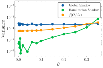
Figure 16: The scaling of variance of estimating $H=V_{H}LV_{H}^{\dagger}$ when using $V_{H}=e^{iP\theta}$ to perform Hamiltonian shadow estimation. $L$ is a non-degenerate real diagonal matrix to represent eigenvalues of the Hamiltonian. The target state is a four-qubit GHZ state and the experiment times is set to be $K=1000$. The value of every point is chosen by taking the median of ten independently sampled $P$.

Proposition 5 is just one situation where the Hamiltonian shadow map becomes invertible caused by eigenstates, there are many other scenarios in which $X_{H}$ is not invertible or has zero off-diagonal elements. An example is shown in Sec. D.2, where $V_{H}=h^{\otimes N}$ and $(X_{H})_{i,j}=2^{-N}$ for all $i$ and $j$. Note that, we can develop a simpler criterion to decide whether $X_{H}$ is invertible or not. As $X_{H}=(V_{H}^{\mathrm{sq}})^{T}V_{H}^{\mathrm{sq}}$, deciding whether $X_{H}$ is invertible or not is equivalent to deciding whether $V_{H}^{\mathrm{sq}}$ is invertible or not.

F.4 Target State

Until now, all discussions are about the evolution unitary $e^{-iHt}$ and measurement. It seems that the reversibility of Hamiltonian shadow map is not related with the target state $\rho$. This is counter-intuitive as if the state is a thermal state $\rho=\frac{e^{-\beta H}}{\Tr(e^{-\beta H})}$, it does not change under Hamiltonian evolution, $e^{-iHt}\rho e^{iHt}=\rho$. Therefore, the final computational basis measurements can only estimate the diagonal terms of $\rho$, and the Hamiltonian shadow seems to be not tomography-complete. While we surprisingly find that this is not the case!

The reason is simple while interesting. Since the Hamiltonian shadow protocol allows us to have the complete information of the Hamiltonian, the unitary $V_{H}$ is also known. If the state commutes with the Hamiltonian, it has the form of $\rho=V_{H}LV_{H}^{\dagger}$, where $L$ is a positive diagonal matrix. Thus, when $V_{H}$ is known, there are only $2^{N}$ unknown parameters to determine $\rho$. As there are also $2^{N}$ diagonal elements of $\rho$, it is possible that one can reconstruct the whole density matrix $\rho$ with only its diagonal elements. Here we will show that the Hamiltonian shadow can do this task directly.

Proposition 6.

If the target state commutes with the Hamiltonian, $[H,\rho]=0$, the Hamiltonian shadow protocol also gives the unbiased estimator of $\rho$,

$$\mathbb{E}_{t,b}\left[V_{H}\mathcal{N}^{-1}\left(\overline{\Lambda}_{t}V_{H}^{\dagger}\outerproduct{b}{b}V_{H}\Lambda_{t}\right)V_{H}^{\dagger}\right]=\rho$$ (87)

Proof.

To prove the Hamiltonian shadow also works for the case of $[H,\rho]=0$, we just need to prove

$$\mathbb{E}_{t,b}\left[\mathcal{N}^{-1}\left(\overline{\Lambda}_{t}V_{H}^{\dagger}\outerproduct{b}{b}V_{H}\Lambda_{t}\right)\right]=L.$$ (88)

Instituting Born’s rule and the condition of $\rho=V_{H}LV_{H}^{\dagger}$, we have

$$\mathbb{E}_{t,b}\left[\mathcal{N}^{-1}\left(\overline{\Lambda}_{t}V_{H}^{\dagger}\outerproduct{b}{b}V_{H}\Lambda_{t}\right)\right]= \mathbb{E}_{t}\left[\sum_{b}\bra{b}e^{-iHt}\rho e^{iHt}\ket{b}\mathcal{N}^{-1}\left(\overline{\Lambda}_{t}V_{H}^{\dagger}\outerproduct{b}{b}V_{H}\Lambda_{t}\right)\right]$$ (89)

$$= \sum_{b}\bra{b}V_{H}LV_{H}^{\dagger}\ket{b}\mathcal{N}^{-1}\left(\mathbb{E}_{t}\overline{\Lambda}_{t}V_{H}^{\dagger}\outerproduct{b}{b}V_{H}\Lambda_{t}\right)$$

$$= \sum_{b}\bra{b}V_{H}LV_{H}^{\dagger}\ket{b}\mathcal{N}^{-1}\left[\sum_{i}\left(V_{H}^{\dagger}\outerproduct{b}{b}V_{H}\right)_{i,i}\outerproduct{i}{i}\right]$$

$$= \sum_{b}\sum_{k}(V_{H})_{b,k}L_{k,k}(V_{H}^{\dagger})_{k,b}\sum_{i,j}(X_{H}^{-1})_{i,j}\left(V_{H}^{\dagger}\outerproduct{b}{b}V_{H}\right)_{j,j}\outerproduct{i}{i}$$

$$= \sum_{i,j,k}\sum_{b}\absolutevalue{(V_{H})_{b,k}}^{2}\absolutevalue{(V_{H})_{b,j}}^{2}(X_{H}^{-1})_{i,j}L_{k,k}\outerproduct{i}{i}$$

$$= \sum_{i,j,k}\left[(V_{H}^{\mathrm{sq}})^{T}V_{H}^{\mathrm{sq}}\right]_{k,j}(X_{H}^{-1})_{i,j}L_{k,k}\outerproduct{i}{i}$$

$$= \sum_{i,j,k}(X_{H})_{k,j}(X_{H}^{-1})_{j,i}L_{k,k}\outerproduct{i}{i}$$

$$= \sum_{i,k}\delta_{i,k}L_{k,k}\outerproduct{i}{i}$$

$$= \sum_{i}L_{i,i}\outerproduct{i}{i}=L,$$

where the third equal sign is due to the property of first-order integral of diagonal random unitary, where all the off-diagonal terms are twirled out; the fourth to the last equal sign is derived using the fact that $X_{H}$ and $X_{H}^{-1}$ are both real symmetric matrices; the third to the last equal sign is derived using a simple fact that $X_{H}X_{H}^{-1}=\mathbb{I}$. ∎

References

Bernien et al. [2017]H. Bernien, S. Schwartz,
A. Keesling, H. Levine, A. Omran, H. Pichler, S. Choi, A. S. Zibrov, M. Endres, M. Greiner,
V. Vuletić, and M. D. Lukin, Probing many-body dynamics on a 51-atom quantum
simulator, Nature 551, 579 (2017).
Ebadi et al. [2021]S. Ebadi, T. T. Wang,
H. Levine, A. Keesling, G. Semeghini, A. Omran, D. Bluvstein, R. Samajdar, H. Pichler, W. W. Ho, S. Choi, S. Sachdev,
M. Greiner, V. Vuletić, and M. D. Lukin, Quantum phases of matter on a 256-atom programmable
quantum simulator, Nature 595, 227 (2021).
Daley et al. [2022]A. J. Daley, I. Bloch,
C. Kokail, S. Flannigan, N. Pearson, M. Troyer, and P. Zoller, Practical quantum advantage in quantum simulation, Nature 607, 667 (2022).
Evered et al. [2023]S. J. Evered, D. Bluvstein,
M. Kalinowski, S. Ebadi, T. Manovitz, H. Zhou, S. H. Li, A. A. Geim, T. T. Wang, N. Maskara,
H. Levine, G. Semeghini, M. Greiner, V. Vuletić, and M. D. Lukin, High-fidelity parallel entangling gates on a neutral-atom quantum
computer, Nature 622, 268 (2023).
Aidelsburger et al. [2015]M. Aidelsburger, M. Lohse,
C. Schweizer, M. Atala, J. T. Barreiro, S. Nascimbène, N. R. Cooper, I. Bloch, and N. Goldman, Measuring the chern number of hofstadter bands with ultracold
bosonic atoms, Nature Physics 11, 162 (2015).
Smits et al. [2018]J. Smits, L. Liao,
H. T. C. Stoof, and P. van der Straten, Observation of a space-time crystal in
a superfluid quantum gas, Phys. Rev. Lett. 121, 185301 (2018).
Semeghini et al. [2021]G. Semeghini, H. Levine,
A. Keesling, S. Ebadi, T. T. Wang, D. Bluvstein, R. Verresen, H. Pichler, M. Kalinowski, R. Samajdar, A. Omran, S. Sachdev, A. Vishwanath, M. Greiner, V. Vuletić, and M. D. Lukin, Probing topological spin liquids on a programmable quantum simulator, Science 374, 1242 (2021).
Randall et al. [2021]J. Randall, C. E. Bradley, F. V. van der
Gronden, A. Galicia,
M. H. Abobeih, M. Markham, D. J. Twitchen, F. Machado, N. Y. Yao, and T. H. Taminiau, Many-body–localized discrete time crystal with a programmable spin-based
quantum simulator, Science 374, 1474 (2021).
Léonard et al. [2023]J. Léonard, S. Kim,
J. Kwan, P. Segura, F. Grusdt, C. Repellin, N. Goldman, and M. Greiner, Realization of a fractional quantum hall state with ultracold atoms, Nature 619, 495 (2023).
Hart et al. [2015]R. A. Hart, P. M. Duarte,
T.-L. Yang, X. Liu, T. Paiva, E. Khatami, R. T. Scalettar, N. Trivedi, D. A. Huse, and R. G. Hulet, Observation of antiferromagnetic
correlations in the hubbard model with ultracold atoms, Nature 519, 211 (2015).
Chiu et al. [2019]C. S. Chiu, G. Ji, A. Bohrdt, M. Xu, M. Knap, E. Demler, F. Grusdt,
M. Greiner, and D. Greif, String patterns in the doped hubbard model, Science 365, 251 (2019).
Hartke et al. [2020]T. Hartke, B. Oreg,
N. Jia, and M. Zwierlein, Doublon-hole correlations and fluctuation thermometry in a
fermi-hubbard gas, Phys. Rev. Lett. 125, 113601 (2020).
Ji et al. [2021]G. Ji, M. Xu, L. H. Kendrick, C. S. Chiu, J. C. Brüggenjürgen, D. Greif, A. Bohrdt, F. Grusdt, E. Demler, M. Lebrat, and M. Greiner, Coupling a mobile hole to an antiferromagnetic spin background: Transient
dynamics of a magnetic polaron, Phys. Rev. X 11, 021022 (2021).
Martinez et al. [2016]E. A. Martinez, C. A. Muschik, P. Schindler,
D. Nigg, A. Erhard, M. Heyl, P. Hauke, M. Dalmonte,
T. Monz, P. Zoller, and R. Blatt, Real-time dynamics of lattice gauge theories with a few-qubit
quantum computer, Nature 534, 516 (2016).
Yang et al. [2020]B. Yang, H. Sun, R. Ott, H.-Y. Wang, T. V. Zache, J. C. Halimeh, Z.-S. Yuan, P. Hauke, and J.-W. Pan, Observation of gauge invariance in a 71-site bose–hubbard quantum
simulator, Nature 587, 392 (2020).
Paulson et al. [2021]D. Paulson, L. Dellantonio, J. F. Haase, A. Celi,
A. Kan, A. Jena, C. Kokail, R. van Bijnen, K. Jansen, P. Zoller, and C. A. Muschik, Simulating
2d effects in lattice gauge theories on a quantum computer, PRX Quantum 2, 030334 (2021).
Meth et al. [2023]M. Meth, J. F. Haase,
J. Zhang, C. Edmunds, L. Postler, A. Steiner, A. J. Jena, L. Dellantonio, R. Blatt,
P. Zoller, et al., Simulating 2d lattice gauge
theories on a qudit quantum computer, arXiv preprint arXiv:2310.12110 (2023).
Hu et al. [2019]M.-G. Hu, Y. Liu, D. D. Grimes, Y.-W. Lin, A. H. Gheorghe, R. Vexiau, N. Bouloufa-Maafa, O. Dulieu, T. Rosenband, and K.-K. Ni, Direct
observation of bimolecular reactions of ultracold krb molecules, Science 366, 1111 (2019).
Burchesky et al. [2021]S. Burchesky, L. Anderegg,
Y. Bao, S. S. Yu, E. Chae, W. Ketterle, K.-K. Ni, and J. M. Doyle, Rotational coherence times of polar
molecules in optical tweezers, Phys. Rev. Lett. 127, 123202 (2021).
Kiczynski et al. [2022]M. Kiczynski, S. K. Gorman, H. Geng,
M. B. Donnelly, Y. Chung, Y. He, J. G. Keizer, and M. Y. Simmons, Engineering topological states in atom-based semiconductor quantum dots, Nature 606, 694 (2022).
Wang et al. [2022]X. Wang, E. Khatami,
F. Fei, J. Wyrick, P. Namboodiri, R. Kashid, A. F. Rigosi, G. Bryant, and R. Silver, Experimental realization
of an extended fermi-hubbard model using a 2d lattice of dopant-based quantum
dots, Nature Communications 13, 6824 (2022).
Elben et al. [2018]A. Elben, B. Vermersch,
M. Dalmonte, J. I. Cirac, and P. Zoller, Rényi entropies from random quenches in atomic hubbard
and spin models, Phys. Rev. Lett. 120, 050406 (2018).
Elben et al. [2019]A. Elben, B. Vermersch,
C. F. Roos, and P. Zoller, Statistical correlations between locally
randomized measurements: A toolbox for probing entanglement in many-body
quantum states, Phys. Rev. A 99, 052323 (2019).
Brydges et al. [2019]T. Brydges, A. Elben,
P. Jurcevic, B. Vermersch, C. Maier, B. P. Lanyon, P. Zoller, R. Blatt, and C. F. Roos, Probing rényi
entanglement entropy via randomized measurements, Science 364, 260 (2019).
Islam et al. [2015]R. Islam, R. Ma, P. M. Preiss, M. Eric Tai, A. Lukin, M. Rispoli, and M. Greiner, Measuring entanglement entropy in a quantum many-body system, Nature 528, 77 (2015).
Elben et al. [2020]A. Elben, R. Kueng,
H.-Y. R. Huang, R. van Bijnen, C. Kokail, M. Dalmonte, P. Calabrese, B. Kraus, J. Preskill, P. Zoller, and B. Vermersch, Mixed-state entanglement from local randomized measurements, Phys. Rev. Lett. 125, 200501 (2020).
Liu et al. [2022]Z. Liu, Y. Tang, H. Dai, P. Liu, S. Chen, and X. Ma, Detecting
entanglement in quantum many-body systems via permutation moments, Phys. Rev. Lett. 129, 260501 (2022).
Rath et al. [2023]A. Rath, V. Vitale,
S. Murciano, M. Votto, J. Dubail, R. Kueng, C. Branciard, P. Calabrese, and B. Vermersch, Entanglement barrier and its symmetry resolution: Theory and experimental
observation, PRX Quantum 4, 010318 (2023).
Imai et al. [2023]S. Imai, G. Tóth, and O. Gühne, Collective randomized measurements in
quantum information processing, arXiv preprint arXiv:2309.10745 (2023).
Mark et al. [2023]D. K. Mark, J. Choi, A. L. Shaw, M. Endres, and S. Choi, Benchmarking quantum simulators using ergodic quantum dynamics, Phys. Rev. Lett. 131, 110601 (2023).
Shaw et al. [2023]A. L. Shaw, Z. Chen, J. Choi, D. K. Mark, P. Scholl, R. Finkelstein, A. Elben, S. Choi, and M. Endres, Benchmarking highly entangled states on a 60-atom analog quantum
simulator, arXiv
preprint arXiv:2308.07914 (2023).
Vermersch et al. [2019]B. Vermersch, A. Elben,
L. M. Sieberer, N. Y. Yao, and P. Zoller, Probing scrambling using statistical correlations between randomized
measurements, Phys. Rev. X 9, 021061 (2019).
Joshi et al. [2022]L. K. Joshi, A. Elben,
A. Vikram, B. Vermersch, V. Galitski, and P. Zoller, Probing many-body quantum chaos with quantum simulators, Phys. Rev. X 12, 011018 (2022).
Elben et al. [2023]A. Elben, S. T. Flammia,
H.-Y. Huang, R. Kueng, J. Preskill, B. Vermersch, and P. Zoller, The randomized measurement toolbox, Nature Reviews Physics 5, 9 (2023).
Huang et al. [2020]H.-Y. Huang, R. Kueng, and J. Preskill, Predicting many properties of a quantum system
from very few measurements, Nature Physics 16, 1050 (2020).
Chen et al. [2021]S. Chen, W. Yu, P. Zeng, and S. T. Flammia, Robust shadow estimation, PRX Quantum 2, 030348 (2021).
Koh and Grewal [2022]D. E. Koh and S. Grewal, Classical Shadows With Noise, Quantum 6, 776 (2022).
Acharya et al. [2021]A. Acharya, S. Saha, and A. M. Sengupta, Informationally complete povm-based
shadow tomography, arXiv preprint arXiv:2105.05992 (2021).
Levy et al. [2021]R. Levy, D. Luo, and B. K. Clark, Classical shadows for quantum process tomography
on near-term quantum computers, arXiv preprint arXiv:2110.02965 (2021).
Wan et al. [2022]K. Wan, W. J. Huggins,
J. Lee, and R. Babbush, Matchgate shadows for fermionic quantum simulation, arXiv preprint arXiv:2207.13723 (2022).
Bu et al. [2022]K. Bu, D. E. Koh,
R. J. Garcia, and A. Jaffe, Classical shadows with pauli-invariant unitary
ensembles, arXiv preprint arXiv:2202.03272 (2022).
Garcia et al. [2021]R. J. Garcia, Y. Zhou, and A. Jaffe, Quantum scrambling with classical shadows, Phys. Rev. Res. 3, 033155 (2021).
Hu et al. [2022]H.-Y. Hu, R. LaRose, Y.-Z. You, E. Rieffel, and Z. Wang, Logical shadow tomography: Efficient estimation of error-mitigated
observables, arXiv preprint arXiv:2203.07263 (2022).
Seif et al. [2023]A. Seif, Z.-P. Cian,
S. Zhou, S. Chen, and L. Jiang, Shadow distillation: Quantum error mitigation with classical shadows
for near-term quantum processors, PRX Quantum 4, 010303 (2023).
Zhan et al. [2023]Y. Zhan, A. Elben,
H.-Y. Huang, and Y. Tong, Learning conservation laws in unknown quantum
dynamics, arXiv preprint arXiv:2309.00774 (2023).
Helsen and Walter [2022]J. Helsen and M. Walter, Thrifty shadow estimation:
re-using quantum circuits and bounding tails, arXiv preprint arXiv:2212.06240 (2022).
Zhou and Liu [2023]Y. Zhou and Q. Liu, Performance analysis of multi-shot
shadow estimation, Quantum 7, 1044 (2023).
Vermersch et al. [2023]B. Vermersch, A. Rath,
B. Sundar, C. Branciard, J. Preskill, and A. Elben, Enhanced estimation of quantum properties with common randomized
measurements, arXiv preprint arXiv:2304.12292 (2023).
Akhtar et al. [2023a]A. A. Akhtar, H.-Y. Hu, and Y.-Z. You, Measurement-induced criticality is
tomographically optimal, arXiv preprint arXiv:2308.01653 (2023a).
Ippoliti and Khemani [2023]M. Ippoliti and V. Khemani, Learnability transitions
in monitored quantum dynamics via eavesdropper’s classical shadows, arXiv preprint arXiv:2307.15011 (2023).
Hu et al. [2023]H.-Y. Hu, S. Choi, and Y.-Z. You, Classical shadow tomography with locally scrambled
quantum dynamics, Phys. Rev. Res. 5, 023027 (2023).
Akhtar et al. [2023b]A. A. Akhtar, H.-Y. Hu, and Y.-Z. You, Scalable and Flexible Classical
Shadow Tomography with Tensor Networks, Quantum 7, 1026 (2023b).
Bertoni et al. [2022]C. Bertoni, J. Haferkamp,
M. Hinsche, M. Ioannou, J. Eisert, and H. Pashayan, Shallow shadows: Expectation estimation using low-depth random
clifford circuits, arXiv preprint arXiv:2209.12924 (2022).
Arienzo et al. [2022]M. Arienzo, M. Heinrich,
I. Roth, and M. Kliesch, Closed-form analytic expressions for shadow estimation
with brickwork circuits, arXiv preprint arXiv:2211.09835 (2022).
Hu and You [2022]H.-Y. Hu and Y.-Z. You, Hamiltonian-driven shadow tomography
of quantum states, Phys. Rev. Res. 4, 013054 (2022).
Zhou and Zhang [2023]T.-G. Zhou and P. Zhang, Efficient classical shadow tomography
through many-body localization dynamics, arXiv preprint arXiv:2309.01258 (2023).
Denzler et al. [2023]J. Denzler, A. A. Mele,
E. Derbyshire, T. Guaita, and J. Eisert, Learning fermionic correlations by evolving with random
translationally invariant hamiltonians, arXiv preprint arXiv:2309.12933 (2023).
Tran et al. [2023]M. C. Tran, D. K. Mark,
W. W. Ho, and S. Choi, Measuring arbitrary physical properties in analog quantum
simulation, Phys. Rev. X 13, 011049 (2023).
McGinley and Fava [2023]M. McGinley and M. Fava, Shadow tomography from
emergent state designs in analog quantum simulators, Phys. Rev. Lett. 131, 160601 (2023).
Van Kirk et al. [2022]K. Van Kirk, J. Cotler,
H.-Y. Huang, and M. D. Lukin, Hardware-efficient learning of quantum many-body
states, arXiv preprint arXiv:2212.06084 (2022).
[63]When directions of Hamiltonian and
measurement basis are parallel or orthorgonal, we cannot uniquely determine
from the trajectories of and the quench