nvblox: GPU-Accelerated Incremental Signed Distance Field Mapping

Abstract

Dense, volumetric maps are essential for safe robot navigation through cluttered spaces, as well as interaction with the environment. For latency and robustness, it is best if these can be computed on-board on computationally-constrained hardware from camera or LiDAR-based sensors. Previous works leave a gap between CPU-based systems for robotic mapping, which due to computation constraints limit map resolution or scale, and GPU-based reconstruction systems which omit features that are critical to robotic path planning. We introduce a library, nvblox, that aims to fill this gap, by GPU-accelerating robotic volumetric mapping, and which is optimized for embedded GPUs. Nvblox delivers a significant performance improvement over the state of the art, achieving up to a $177\times$ speed-up in surface reconstruction, and up to a $31\times$ improvement in distance field computation, and is available open-source.

I Introduction

To navigate and interact with their environment robots typically build an internal representation of the world. Significant research in the past decades [1] has focused on building maps that are both useful for robotic path-planning, and efficient to construct. However, fulfilling these two requirements simultaneously remains challenging.

Various successful systems have emerged for solving the Simultaneous Localization and Mapping (SLAM) problem efficiently [2, 3]. Typically these systems build sparse representations of the environment in order to reach real-time rates, as the main purpose of these systems is to provide a pose estimate of the robot. While this is essential, safe navigation requires not only pose but also information about obstacles in the environment.

Several systems have emerged for building denser representations of the environment on the CPU [4, 5, 6] that are suitable for robotic path-planning. However, the frequency, resolution, and scale at which these systems can operate is limited by the computational burden of 3D reconstruction on a CPU. To address these limitations systems utilizing GPU programming have emerged [7, 8]. These systems, however, have typically focused on reconstruction alone and have omitted features needed in a robotic path-planning context, such as incremental computation of the signed distance field and its gradients, as well as an explicit representation of free space. We aim to address this gap.

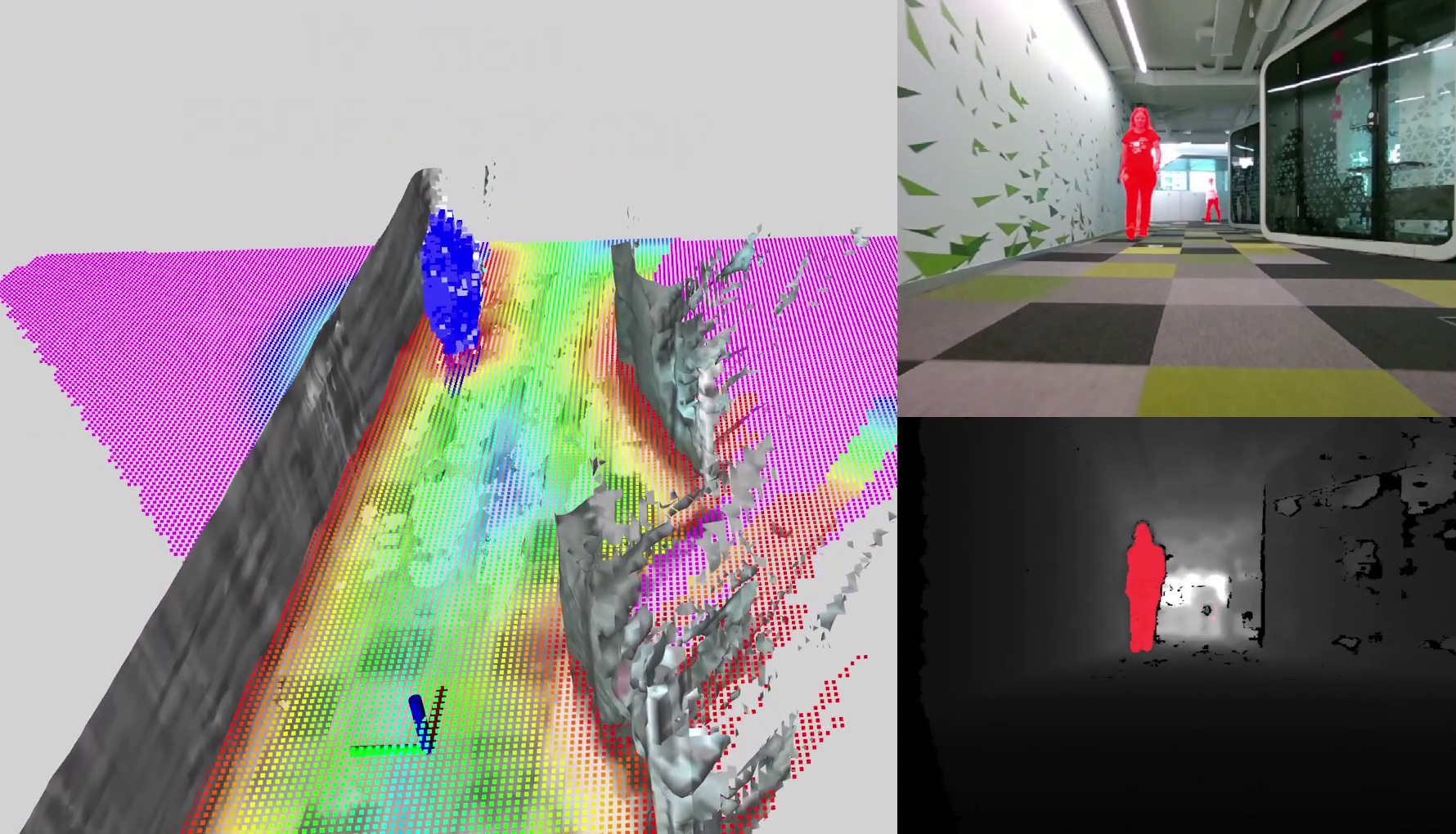
Figure 1: An example of nvblox being used on a ground robot in an office building, showing semantic segmentation of a dynamic obstacle (a person). The image shows a reconstructed mesh, a slice through the distance field, as well as occupancy-probability voxels representing the reconstructed human. All operations to build this reconstruction are performed in real-time on an embedded GPU.

This paper introduces nvblox, a library for volumetric mapping on the GPU, specifically targeted at robotic path-planning. Nvblox produces high-resolution surface reconstructions at real-time rates, even on embedded GPUs. In addition, however, nvblox also produces distance fields, which are a key output for planning collision-free paths. Central to our approach is the use of parallel computation on the GPU for all aspects of the pipeline, including queries. We show the efficacy and efficiency of nvblox on several public datasets, and applied to several robotic use-cases, such as path planning for robot arms, flying robots, and for mapping of dynamic obstacles such as people.

In summary, the contribution of this paper is a GPU-accelerated Signed Distance Field (SDF) library with a convenient and flexible interface. Nvblox fuses in data from RGB-D sensors and/or LiDAR, up to $177\times$ faster in surface reconstruction ( Truncated Signed Distance Field (TSDF)) and between $7\times$ and $63\times$ faster in the distance field ( Euclidean Signed Distance Field (ESDF)) computation than state-of-the-art CPU-based methods [9, 4]. The library is made available open-source in both ROS1 and ROS2.

II Related Work

Mapping is a well-explored problem in robotics [1]. We can categorize robotic mapping approaches into two broad categories: sparse and dense. Sparse methods focus on creating a map representation for pose estimation and localization while dense methods focus on reconstructing objects or the geometry of the environment.

Systems for dense mapping can be organized by the underlying representation used to represent the environment. LSD-SLAM [10] and DVO-SLAM [11] build a map consisting of keyframe depth-maps. Kintinuous [12] and ElasticFusion [8] build reconstructions in the form of a deformable mesh and collection of surfels respectively. More recently, Kimera [13] builds a semantic mesh of the environment. These approaches build visually compelling reconstructions. However, they produce maps that are less suited to robotic path-planning because surfaces alone are reconstructed; parts of the environment that are free of objects, and are therefore navigable, are not captured in these system’s representations of the environment.

Recently, reconstruction systems based on neural radiance fields have gained significant attention [14]. The original offline approach has seen dramatic speedups [15], leading to implementations that generate reconstructions in real-time [16, 17]. There is early work into the use of the resulting maps for path-planning [18, 19]. Currently, however, NERF-based planning approaches perform the expensive reconstruction step offline, limiting their applicability to mobile robotics where mapping and planning are required to occur concurrently.

Voxel-based methods build reconstructions that are well-suited to robot path-planning tasks. Voxels capture some reconstructed quantity over the volume or 3D space, and can therefore represent free-space, not only surfaces. The most common approach to volumetric reconstruction is occupancy grid mapping [20] and its efficient implementation in 3D, Octomap [5]. These approaches are among the most widely used in robotic mapping and are the default in common robotics toolboxes [21, 22].

Another popular approach to volumetric mapping utilizes a voxelized TSDF. This approach was popularized by KinectFusion [7] which generates compelling surface reconstructions using consumer-grade depth cameras. The original, fixed-grid-based approach was extended to use spatially hashed voxels by Niessner et. al. [23]. Voxblox [4] follows the approach of voxel-hashing but adds ESDF computation, a feature of particular importance for robotic path-planning. Voxblox has been used in many follow on works which have used it for planning [24, 25], as well as extended its mapping capabilities, for example for global mapping [6] and semantic mapping [26]. Despite its success, voxblox is limited in the resolution of maps it builds due to the cubic scaling in computational complexity as the resolution increases.

Several works have followed in voxblox’s footsteps, mainly focusing on decreasing the ESDF generation error and runtime. Voxfield [27], for example, removes the inaccuracies caused by voxblox’s quasi-Euclidean distance estimation and improve the ESDF runtime by up to 42%. Similarly, FIESTA uses occupancy instead of TSDF as the mapping representation, and speeds up voxblox’s ESDF computation by $4\times$ while also computing full Euclidean distance. Nvblox also uses full Euclidean distance, therefore reducing the ESDF error, but is on average $31\times$ faster than voxblox.

By improving existing methods through GPU acceleration, we create a library that provides a suitable representation for a large body of path planners and other downstream applications, while reducing runtime and allowing the creation of higher-resolution maps on the robot.

III Problem Statement

Given a sequence of measurements from an RGB-D camera and/or a LiDAR, we aim to build a volumetric reconstruction of the scene. Our reconstruction is a function $\Phi:\mathbb{R}^{3}\to\phi$, which maps a point in 3D space to some mapped quantity $\phi$, for example distance, occupancy, or color. This function is voxelized, i.e. represented as a sparse set of samples on a regular 3D grid, where samples are allocated in regions of space that have been observed by the sensor. We assume that at time step $i$ the sensor frame $C^{i}$ is localized in a frame $L$ such that we have access to the sensor pose $\mathbf{T}_{LC^{i}}\in\text{SE}(3)$. Observations take the form of depth maps and color images. A depth map is $\mathcal{D}:\Omega\to d$, where $d\in\mathbb{R}$ is a depth value in meters. The domain $\Omega$ is the image plane in the case of depth cameras, and the beam angles in the case of rotating LiDARs. Similarly, color images are $\mathcal{C}:\Omega\to c$ where $c\in\mathbb{R}^{3}$. In the remainder of this paper, we will refer to observations from both camera and LiDAR as images and treat the two equally.

The output quantities we intend to compute are the surface reconstruction (expressed as either occupancy or the TSDF) and the distance field that’s used for collision computation (expressed as the ESDF).

IV System architecture description

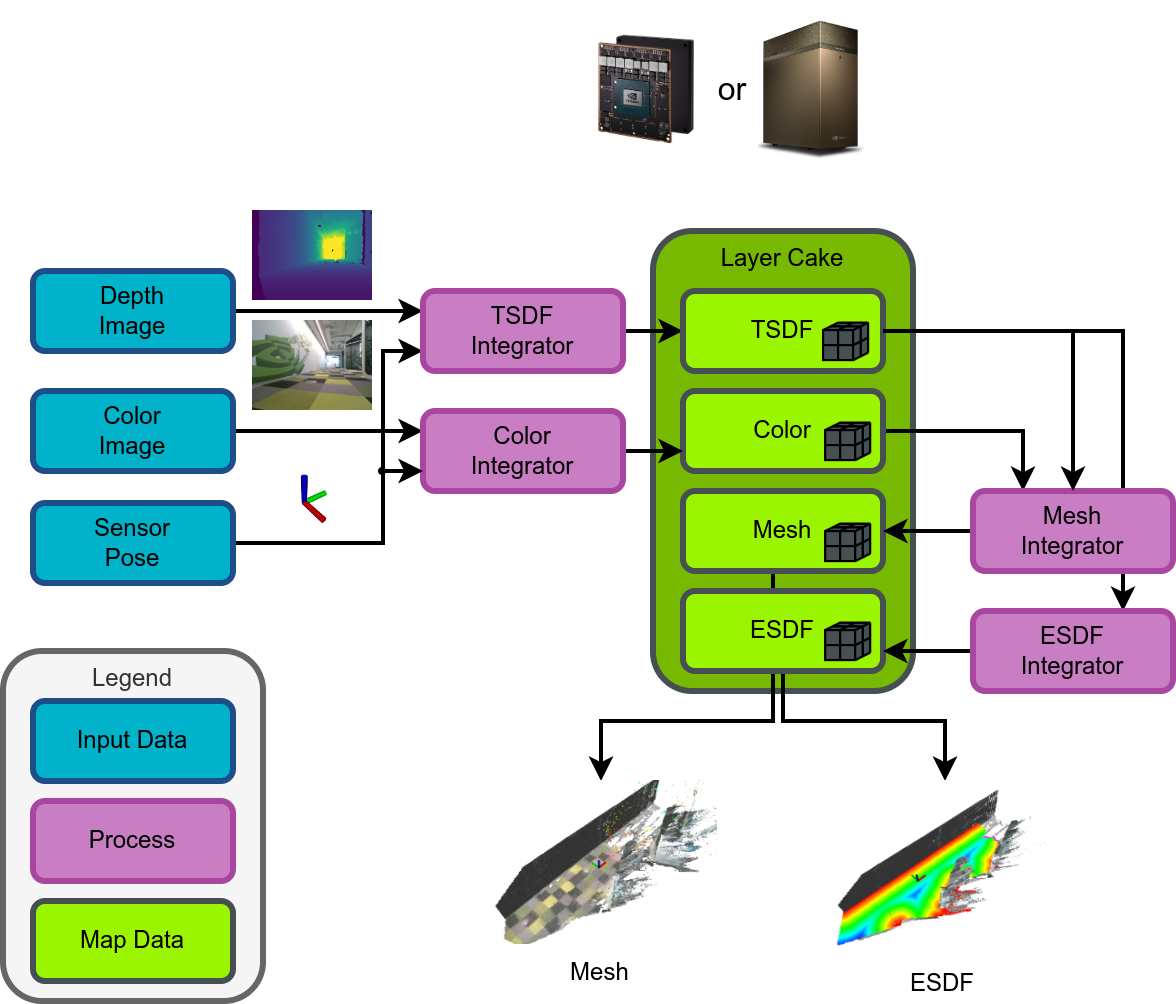
Figure 2: The system architecture of nvblox, configured for TSDF mapping from an RGB-D camera sensor. The reconstructed map (called a LayerCake) is composed of co-located and aligned 3D voxel grids. Input depth-maps and color images are integrated into the TSDF and Color voxel layers, from which voxel grids containing the ESDF and a mesh reconstruction are derived. See Sec. IV for details.

The architecture of nvblox is shown in Fig. 2. The system consists of multiple components: the reconstructed map, which contains several Layers, processes that add sensor data to the map called Frame Integrators, as well as components that transform one layer type into another, such as mesh and ESDF integrators. We discuss these components in more detail below.

IV-A The Map

Our reconstruction is represented as several overlapping 3D voxel grids, called Layers, following [4]. Each Layer of the map stores a different type of (user-defined) data for overlapping volumes of 3D space. The map is sparse, such that voxels are only allocated in regions of 3D space that are observed during mapping. This sparsity is achieved using a two-level hierarchy, following [23]. The first level is a hash table that maps 3D grid indices to VoxelBlocks. In nvblox this hash table can be queried in GPU kernels using an interface based on stdgpu [28]. In the second layer, each VoxelBlock contains a small group of densely allocated voxels which are stored contiguously in GPU memory, in our case, in cubes of $8\times 8\times 8$ voxels to better fit into CUDA’s thread limits. This contiguous storage leads to a higher degree of coalescing during loads in kernels.

The map is designed to be extended with new layers. To create a new Layer, a user needs to specify the contents of a single voxel. The library generates the definitions for the corresponding block-hashed voxel grid at compile time, as well as CPU and GPU interfaces such that the voxel grid is accessible in CUDA kernels. The nvblox library comes with commonly used Layers defined: TSDF, ESDF, occupancy, color, and meshes. The data structure can be extended for storing other types of information, like semantic labels [26].

IV-B Frame Integration

Incoming sensor data is added to the reconstruction stored in one of the map layers. This occurs in several steps. We first ray trace the VoxelBlock-grid on the GPU to determine which VoxelBlocks are in view using [29] and allocate those not yet in the map. We then project each voxel in view into the depth image:

$$d=\mathcal{D}[\pi_{\text{sensor}}(\mathbf{T}_{CL}\mathbf{p}_{L})]$$ (1)

where $d\in\mathbb{R}$ is the sampled depth value, $\mathbf{T}_{CL}$ is the camera pose with respect to the Layer, and $\mathbf{p}_{L}$ is the voxel center position in the Layer coordinate frame. The sensor projection function for a camera is $\pi_{\text{sensor}}$ is

$$\pi_{\text{camera}}(\mathbf{p}_{C})=\frac{1}{p_{C,z}}\left[\begin{array}[]{ccc}f_{u}&0&c_{u}\\ 0&f_{v}&c_{v}\end{array}\right]\left[\begin{array}[]{c}p_{C,x}\\ p_{C,y}\\ 1\end{array}\right]$$ (2)

where $f_{u}$, $f_{v}$, $c_{u}$, $c_{v}$ are calibrated pinhole camera intrinsics, and for LiDAR

$$\pi_{\text{lidar}}(\mathbf{p}_{C})=\left[\begin{array}[]{c}(\tan^{-1}(p_{C,y}/p_{C,x})-\theta_{\text{start}})*\alpha_{\theta}\\ (\cos^{-1}(p_{C,z}/r)-\phi_{\text{start}})*\beta_{\phi}\end{array}\right],$$ (3)

where $\theta_{\text{start}}$, $\phi_{\text{start}}$ are the minimum polar and azimuth angles, and $\alpha_{\theta}$ and $\beta_{\phi}$ are measured in pixels-per-radian and are calculated by dividing the Field of View (FoV) by the number of steps/beams in the relevant dimension. The function $\mathcal{D}[\mathbf{u}]$ indicates sampling the depth image $\mathcal{D}$ at image-coordinates $\mathbf{u}$. For a camera, we sample using nearest-neighbor, and for LiDAR-based depth images, which can be very sparse, we use linear interpolation with modifications to avoid interpolating over foreground-background boundaries.

To update each voxel in view, we call a user-supplied update functor on the GPU with the sampled depth image value, in parallel over all blocks. We provide update functors for TSDF, occupancy, and color fusion, but the library is designed to accept additional ones.

IV-C Mesh Computation

While the ESDF is the primary output of interest for path-planning, a mesh is useful for visualizing the scene. We compute a triangular mesh of the reconstructed scene from the TSDF using Marching Cubes [30]. The mesh is computed incrementally, that is, periodically areas of the map that have been updated during reconstruction are re-meshed. We exploit the structure of our map to perform meshing efficiently on the GPU. We run Marching Cubes in each VoxelBlock using a CUDA thread block, with each CUDA thread calculating the mesh triangles that touch a single voxel. We then run an additional kernel to calculate triangles across block boundaries. The operation is largely data-parallel and therefore efficient to perform on the GPU, which allows frequent re-meshing in real-time.

IV-D ESDF Computation

The Truncated Signed Distance Field (TSDF) contains projective distances up to a small truncation distance. For path planning applications we require Euclidean distances (as opposed to projective distances) and for greater distances than the truncation band. For a discussion on why a TSDF is insufficient for this, we refer the reader to [31].

Our ESDF computation approach has several requirements. It must be both incremental and parallelized on the GPU. Our previous work, voxblox [4], computed an incremental quasi-Euclidean ESDF, where each voxel had 26-connectivity to its neighbors and distances were approximated as either $1$ or $\sqrt{2}$. The quasi-Euclidean distance assumption was taken to limit the number of updates, as the incremental update was done in 3D with a brushfire algorithm [32], which can lead to a large number of updates, even with small changes to the voxel distance. The quasi-Euclidean distance is an undesirable approximation that lowers the overall accuracy of the distance field. In contrast, nvblox computes the exact Euclidean distance without this approximation.

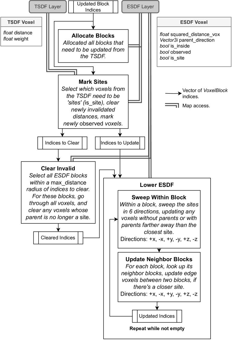
Figure 3: Overall flow of the incremental ESDF computation on the GPU. The algorithm does as much of the update in parallel as possible, iteratively finding all the blocks that need to be updated, and then running kernels on all blocks in parallel.

In order to create a highly parallel ESDF computation algorithm, we base our work in spirit on the Parallel Banding Algorithm (PBA) proposed by Cao et al. [33]. The overall flow of the algorithm is shown in Fig. 3 and visualized step-by-step in Fig. 5. The general intuition of the algorithm is to do highly parallelized operations on every VoxelBlock based on the contents of its voxels.

First, in Allocate Blocks, a TSDF layer and a list of updated VoxelBlocks are taken as input. Generally, TSDF blocks that were changed since the last iteration of ESDF integration are considered updated (this allows us to run the ESDF update slower than sensor rate). Any new VoxelBlocks are allocated in the ESDF as needed.

The next step is Mark Sites. A site is defined as a voxel that can be a parent in the obstacle calculation; therefore a voxel on the surface boundary. Children of this voxel would be voxels whose closest surface boundary is the site in question, as illustrated in Fig. 4. We consider voxels to be sites if their TSDF distance is within a threshold $\epsilon$ of the zero crossing (see Fig. 5(b)). In addition to marking sites, this function ensures consistency between the ESDF and TSDF maps, and there are two general cases we need to handle: newly occupied or newly observed voxels, and newly free voxels. Newly occupied voxels simply take on their TSDF distance values and are added to Indices to Update. However, newly free voxels need to have their distances reset to maximum (as we do not have a valid distance estimate), and if they were previously sites, we need to ensure all their children are invalidated. Such voxels have their blocks are added to Indices to Clear.

Next, we Clear Invalid. The idea is to find voxels whose parents are no longer a site, and therefore need distance recomputation. We select a subset of the map that is within the maximum ESDF distance of the block Indices to Clear, and then check that each voxel still has a valid parent. If the parent is no longer marked as a site, then the voxel distance is set to maximum, and the block index is added to Cleared Indices. This would seem an expensive operation but in practice, it is faster to check all potentially affected blocks in parallel than follow an iterative approach.

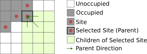
Figure 4: “Sites” are voxels on the surface boundary, and its children are any voxels which are closer to that voxel than any other site. Each child stores its parent direction - the direction that points to the parent site location (only shown for the closest 3 voxels here for clarity).

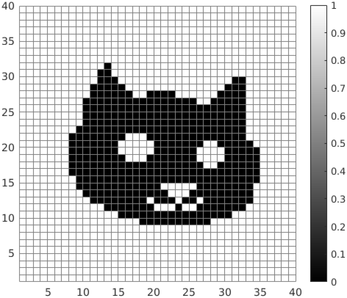
(a) Occupancy

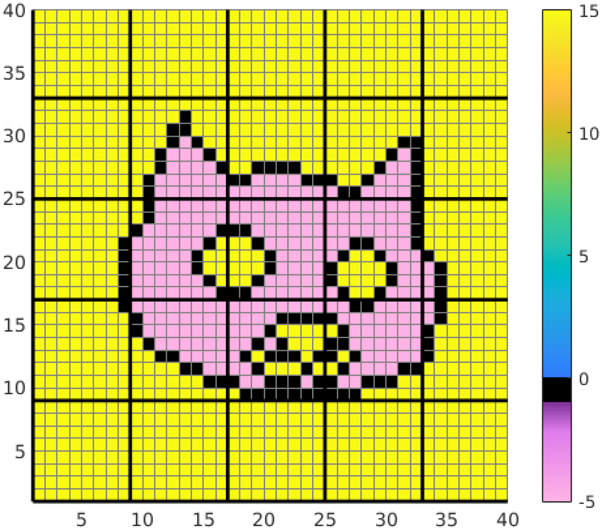
(b) Marking

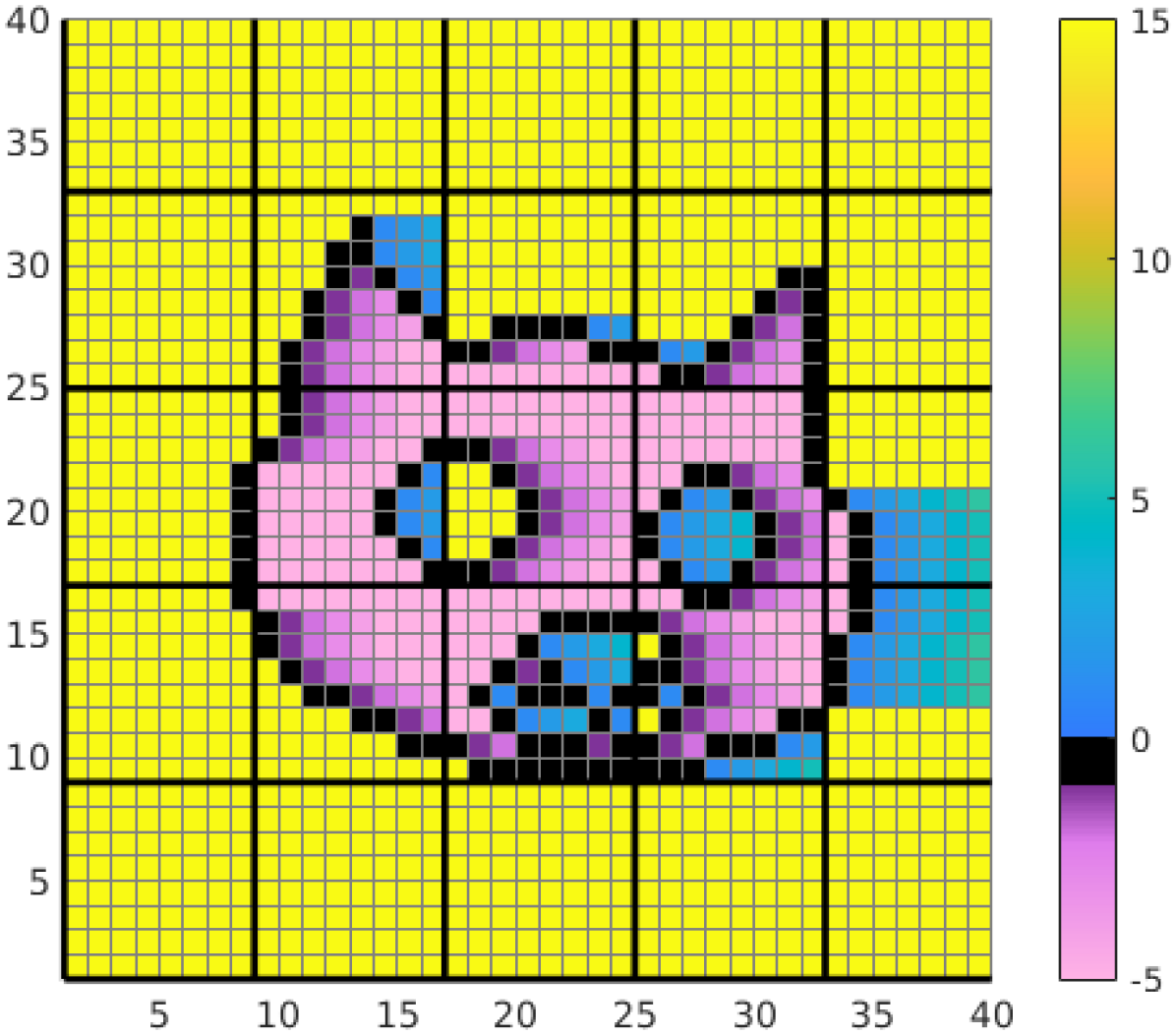
(c) $X+$ Sweep

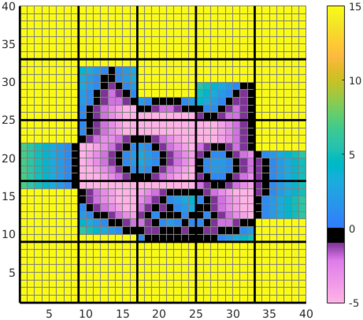
(d) $X-$ Sweep

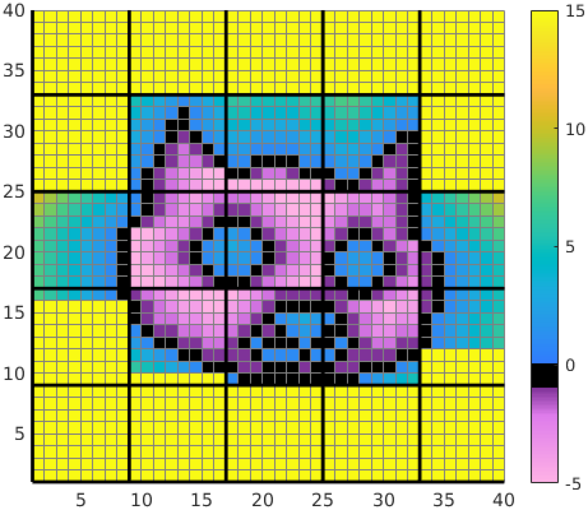
(e) $Y+$ Sweep

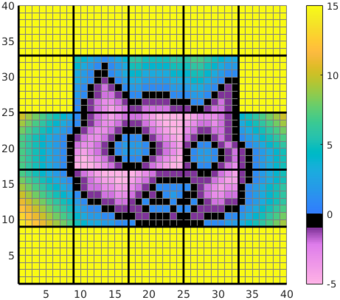
(f) $Y-$ Sweep

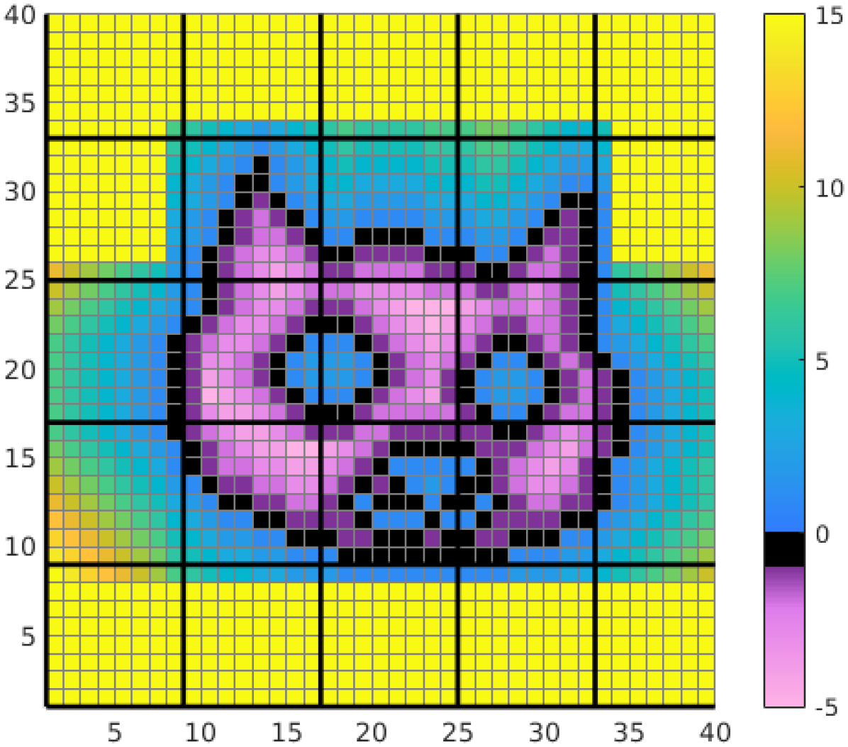
(g) Neighbor Border Copies

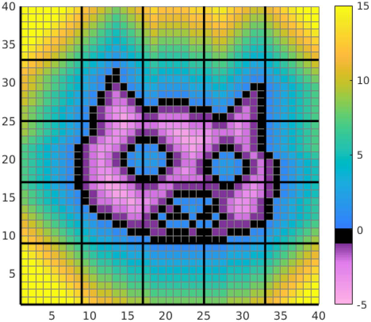
(h) Final Sweeps

Figure 5: Marking and lowering, shown step-by-step on an image. Occupancy is used instead of the TSDF for simplicity, and we show only a 2D implementation of the algorithm (while a 3D version is presented in this paper). The bold lines represent VoxelBlock boundaries. The general idea of the algorithm is to iteratively compute correct distance values within a VoxelBlock, and then communicate distance information across VoxelBlock boundaries to neighbors.

	Component Runtime (ms)
	Replica [34]								Redwood [35]
	Desktop		Laptop		Jetson				Desktop		Laptop		Jetson
Component	nvblox	vox.	nvblox	vox.	nvblox	vox.	Speedup		nvblox	vox.	nvblox	vox.	nvblox	vox.	Speedup
ESDF	1.9	163.2	3.6	291.5	8.4	231.6	×63		1.5	29.1	2.6	46.5	4.2	38.7	×16
TSDF	0.4	-	0.6	-	1.6	-	×174		0.2	-	0.2	-	0.5	-	×177
Color	1.7	-	2.5	-	4.2	-	-		1.1	-	1.6	-	2.4	-	-
TSDF+Color	2.1	86.7	3.2	106.6	5.8	226.7	×38		1.3	38.4	1.8	33.6	2.9	76.7	×25
Mesh	1.6	6.2	4.0	12.0	12.3	15.4	×3		0.6	12.7	1.5	15.8	2.7	23.0	×13

TABLE I: Timings for various components of nvblox and voxblox during reconstruction of the Replica [34] and Redwood [35] datasets at 5 cm resolution. Timings are averaged over 8 sequences for Replica, and 5 sequences for Redwood (see Sec. V-A for details). Speedup is how many times faster nvblox is than voxblox. Some values are missing as voxblox does not separate TSDF and color integration; because of this, the TSDF speedup is assuming only surface integration in nvblox vs. both surface and color for voxblox (which is relevant in colorless scenarios like LiDAR integration).

Finally, the Lower ESDF stage consists of two steps in a loop (this is called Lowering since it exclusively lowers the ESDF voxel distance). The first is Sweeping Within a Block through each VoxelBlock once in each axis direction, in parallel. This is similar to the PBA [33] approach, except confined to the block boundaries. Fig. 5(c) shows the first positive sweep within the block: each neighbor in the $X+$ direction is updated if there is a shorter distance to the site through that direction. We then repeat the process in $X-$, $Y+$, $Y-$, $Z+$ and $Z-$. This is done over all affected VoxelBlocks in a single kernel call, and at the end of the 6 sweeps, the distances within a VoxelBlock are correct, given the current values on each VoxelBlock’s boundaries.

Then we attempt to reconcile the differences between VoxelBlocks by Updating Neighbor Blocks by communicating across block boundaries. Values are propagated from the edges of one block to another if there is a shorter distance to a site through the neighboring block (see Fig. 5(g)).

If the last stage required communication over VoxelBlock borders, those blocks require another sweep. We repeat the sweep-neighbor update loop until no more blocks can be updated, which in practice usually terminates in few iterations.

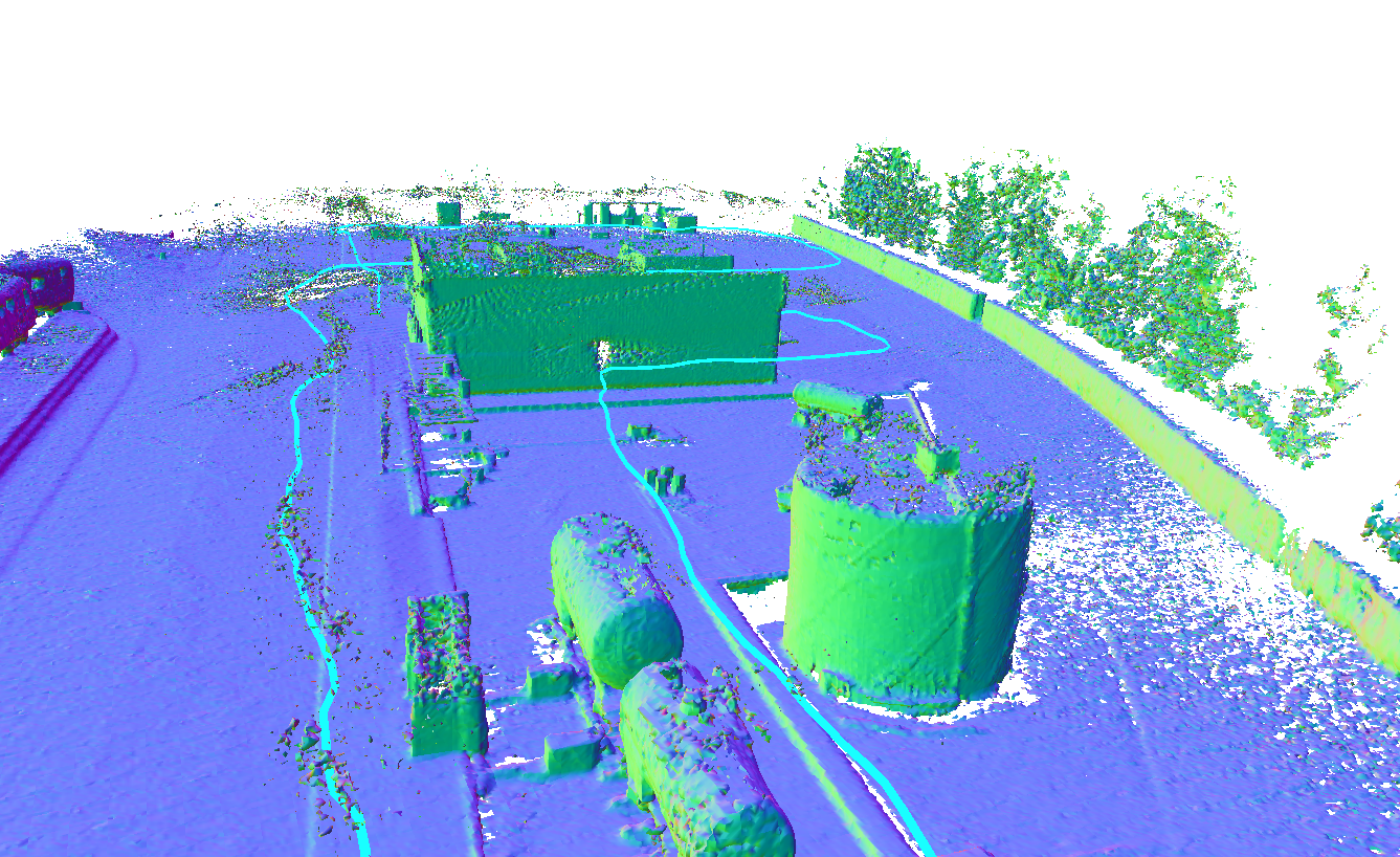
Figure 6: An example of the output from a large-scale flying robot dataset. The integration time is less than 7 ms for a 64-beam LiDAR with 25 meter maximum range at 10 cm resolution on a laptop, and less than 20 milliseconds on the Jetson, allowing us to run at at least $2\times$ real time.

		Median ESDF Error (m)				ESDF Runtime (ms) (speedup)
Dataset	Sequence	nvblox	voxblox	Fiesta		nvblox	voxblox	Fiesta
Redwood [3]	apartment	0.04	0.06	0.05		1.7 (×14)	25 (×1)	5.5 (×5)
Redwood [3]	bedroom	0.02	0.05	0.03		1.4 (×15)	22 (×1)	3.4 (×6)
Redwood [3]	boardroom	0.06	0.08	0.06		1.7 (×17)	30 (×1)	4.0 (×8)
Redwood [3]	lobby	0.10	0.10	0.08		2.1 (×16)	34 (×1)	5.2 (×7)
Redwood [3]	loft	0.04	0.08	0.04		1.8 (×26)	48 (×1)	8.4 (×6)
Cow and lady [4]	-	0.09	0.06	0.07		2.8 (×68)	190 (×1)	52 (×4)
Average		0.06	0.07	0.06		1.9 (×31)	58 (×1)	13 (×4)

TABLE II: Accuracy and runtime performance of incremental ESDF generation of the proposed system compared to baselines: voxblox [4], and Fiesta [9]. The systems are compared on the Redwood [35] and Cow and Lady [4] datasets (see Sec. V-A for details). Speedup is the runtime performance increase over voxblox for both methods. On average, nvblox is $7\times$ faster than Fiesta and $31\times$ faster than voxblox.

V Experiments

In this section, we aim to validate the central claim of our paper: that nvblox improves the state-of-the-art in volumetric mapping for robot path planning in terms of run-time performance, without compromising the accuracy of the reconstructed distance field (ESDF). We report timings on 3 different platforms: a desktop computer with an Intel i9 CPU and NVIDIA RTX3090 Ti GPU (Desktop), a laptop computer with an Intel i7 CPU and a RTX3000 Mobile GPU (Laptop), and a Jetson Xavier AGX (Jetson).

V-A System Benchmarking

We evaluate the performance of various modules of nvblox on the Replica Dataset [34] (using the sequences generated in [16]) which provides photorealistic renderings of synthetic rooms, and the Redwood dataset [35] which are real scans of several environments with a consumer depth camera.

Table I shows timings for various modules of our system; TSDF fusion, color fusion, incremental ESDF update and incremental meshing. We perform ESDF generation and meshing every 4 frames. We average timings over the 8 sequences of the Replica Dataset and 5 sequences of the Redwood Dataset.

When compared to our previous work, voxblox [4], which runs on the CPU we see significant speed-ups in all modules of the system. In the case of TSDF and color this is a well-known result, as the GPU has been used to accelerate TSDF mapping since KinectFusion [7]. We show that these speed-ups are also achievable on an embedded GPU, and that similar speed-ups are available for incremental ESDF calculation, which we describe below.

V-B ESDF Timings

We aim to evaluate our central claim of improvement in the state-of-the-art in incremental ESDF calculation. We compare nvblox against voxblox [4], and Fiesta [9], a recent and more performant algorithm. Table II shows timings and ESDF accuracy for our Desktop system. The ESDF distance is computed by generating a ground-truth ESDF at the voxel center locations from the dataset-supplied ground-truth surfaces. We tabulate the median error across the voxels of the reconstruction. Table II shows a significant speedup of $31\times$ with respect to voxblox and $7\times$ with respect to Fiesta. Furthermore, the experiments show that this speed-up does not come at the cost of reduced accuracy.

V-C Query Timings

The primary purpose of mapping in a typical robotic system is to provide collision information to path-planning modules. For many optimization or sampling-based planners, querying the collision status of a state can constitute a significant portion of the total computational cost. Performing these queries on the GPU allows us to take advantage of parallelization, and enables GPU-based path planners, like in [36] and [37]. A query in nvblox takes a collection of 3D points on the GPU and returns their distances to the closest surface and optionally their distance field gradient, by performing an ESDF lookup on the GPU. Table III shows query rates in giga-queries-per-second for an NVIDIA GeForce 3090 Ti as well as a Jetson AGX. The table shows the results for spatially correlated (cor.) and uncorrelated (uncor.) sampling. In correlated sampling, adjacent queries are more likely to fall in the same VoxelBlock, leading to coalesced memory access on the GPU and higher query rates. This is typically the case for robotic use cases where the queries are spatially correlated, for example clustered around the robot’s current location.

	$10^{9}$ Queries per Second
	Desktop			Jetson
Dataset	cor.	uncor.		cor.	uncor.
Redwood (5 sequences)	6.2	3.3		0.8	0.5
Sun3D (6 sequences)	7.3	3.3		0.7	0.3

TABLE III: The number of distance giga-queries per second delivered by nvblox, averaged over several sequences of the Redwood [35] and Sun3D datasets [38]. Even on the Jetson, uncorrelated queries take only 3 nanoseconds per point.

V-D Application examples

To demonstrate the utility of nvblox at various problem scales, we show examples of its use on flying robots, robot arms, and mobile ground robots. Fig. 6 shows the results from reconstructing a dataset collected with a drone [6], which is equipped with a 64-beam Ouster OS1 LiDAR. We use Fast-LIO [39] as a pose estimator and integrate the LiDAR up to a range of 25 meters at a resolution of 5 cm, which requires less than 7 ms per LiDAR scan on a Laptop. This is an example of nvblox’s suitability for large-scale outdoor scenarios, where the resulting 3D ESDF can be used for both global [40] and local planning [41]. The nvblox library has also been used on-board a different flying robot to enable Riemannian Motion Policies which allow reactive navigation at kHz rates [37].

Nvblox is suitable for small-scale problems as well, as shown for high-rate adaptive planning for robot arms in CuRobo [36], where the authors take advantage of nvblox’s fast query speeds directly on GPU to sample vastly more trajectory candidates than previously possible.

Lastly, we show an image from a robot mapping in an office environment Fig. 1. In this example, we use PeopleSemSegnet to segment the reconstruction into the static environment and dynamic elements (humans in this case). Humans are used to feed a separate 3D occupancy grid using a separate OccupancyLayer in nvblox. The result is a two-part reconstruction, where dynamic parts of the scene decay over time, but the static parts of the scene are accurately reconstructed using TSDF fusion.

In general, nvblox is useful not only because it is faster than existing methods, but also because all data is already stored on the GPU. This enables seamless integration with other modules that can take advantage of parallelization or use the GPU, such as path planners or deep learning methods.

VI Conclusion

In conclusion, we introduce nvblox, a library for volumetric mapping on the GPU. The library aims at filling a gap between CPU-based volumetric mapping systems aimed at robotics, which are computationally limited, and GPU-based systems that typically omit features that are important for a robotics use-case. As part of the toolbox we include a novel incremental, GPU-accelerated method for computing the ESDF. The system is optimized for operation on both discrete and embedded GPUs. We provide experiments demonstrating that nvblox is significantly faster both in mapping and distance field computation, as well as query time, than other state-of-the-art approaches.

References

- [1] Cesar Cadena et al. “Past, present, and future of simultaneous localization and mapping: Toward the robust-perception age” In IEEE Transactions on robotics 32.6 IEEE, 2016, pp. 1309–1332
- [2] Raul Mur-Artal, Jose Maria Martinez Montiel and Juan D Tardos “ORB-SLAM: a versatile and accurate monocular SLAM system” In IEEE transactions on robotics 31.5 IEEE, 2015, pp. 1147–1163
- [3] Thomas Schneider et al. “maplab: An open framework for research in visual-inertial mapping and localization” In IEEE Robotics and Automation Letters 3.3 IEEE, 2018, pp. 1418–1425
- [4] Helen Oleynikova et al. “Voxblox: Incremental 3D Euclidean Signed Distance Fields for On-Board MAV Planning” In IEEE/RSJ International Conference on Intelligent Robots and Systems (IROS), 2017
- [5] Armin Hornung et al. “OctoMap: An efficient probabilistic 3D mapping framework based on octrees” In Autonomous robots 34 Springer, 2013, pp. 189–206
- [6] Victor Reijgwart et al. “Voxgraph: Globally consistent, volumetric mapping using signed distance function submaps” In IEEE Robotics and Automation Letters 5.1 IEEE, 2019, pp. 227–234
- [7] Shahram Izadi et al. “Kinectfusion: real-time 3d reconstruction and interaction using a moving depth camera” In Proceedings of the 24th annual ACM symposium on User interface software and technology, 2011, pp. 559–568
- [8] Thomas Whelan et al. “ElasticFusion: Dense SLAM without a pose graph”, 2015 Robotics: ScienceSystems
- [9] Luxin Han, Fei Gao, Boyu Zhou and Shaojie Shen “Fiesta: Fast incremental euclidean distance fields for online motion planning of aerial robots” In 2019 IEEE/RSJ International Conference on Intelligent Robots and Systems (IROS), 2019, pp. 4423–4430 IEEE
- [10] Jakob Engel, Thomas Schöps and Daniel Cremers “LSD-SLAM: Large-scale direct monocular SLAM” In Computer Vision–ECCV 2014: 13th European Conference, Zurich, Switzerland, September 6-12, 2014, Proceedings, Part II 13, 2014, pp. 834–849 Springer
- [11] Christian Kerl, Jürgen Sturm and Daniel Cremers “Dense visual SLAM for RGB-D cameras” In 2013 IEEE/RSJ International Conference on Intelligent Robots and Systems, 2013, pp. 2100–2106 IEEE
- [12] Thomas Whelan et al. “Kintinuous: Spatially extended kinectfusion”, 2012
- [13] Antoni Rosinol, Marcus Abate, Yun Chang and Luca Carlone “Kimera: an open-source library for real-time metric-semantic localization and mapping” In 2020 IEEE International Conference on Robotics and Automation (ICRA), 2020, pp. 1689–1696 IEEE
- [14] Ben Mildenhall et al. “Nerf: Representing scenes as neural radiance fields for view synthesis” In Communications of the ACM 65.1 ACM New York, NY, USA, 2021, pp. 99–106
- [15] Thomas Müller, Alex Evans, Christoph Schied and Alexander Keller “Instant neural graphics primitives with a multiresolution hash encoding” In ACM Transactions on Graphics (ToG) 41.4 ACM New York, NY, USA, 2022, pp. 1–15
- [16] Edgar Sucar, Shikun Liu, Joseph Ortiz and Andrew J Davison “iMAP: Implicit mapping and positioning in real-time” In Proceedings of the IEEE/CVF International Conference on Computer Vision, 2021, pp. 6229–6238
- [17] Zihan Zhu et al. “Nice-slam: Neural implicit scalable encoding for slam” In Proceedings of the IEEE/CVF Conference on Computer Vision and Pattern Recognition, 2022, pp. 12786–12796
- [18] Michael Pantic, Cesar Cadena, Roland Siegwart and Lionel Ott “Sampling-free obstacle gradients and reactive planning in Neural Radiance Fields (NeRF)” In arXiv preprint arXiv:2205.01389, 2022
- [19] Michal Adamkiewicz et al. “Vision-only robot navigation in a neural radiance world” In IEEE Robotics and Automation Letters 7.2 IEEE, 2022, pp. 4606–4613
- [20] Sebastian Thrun “Probabilistic robotics” In Communications of the ACM 45.3 ACM New York, NY, USA, 2002, pp. 52–57
- [21] Steve Macenski, Francisco Martín, Ruffin White and Jonatan Ginés Clavero “The marathon 2: A navigation system” In 2020 IEEE/RSJ International Conference on Intelligent Robots and Systems (IROS), 2020, pp. 2718–2725 IEEE
- [22] Steve Macenski, David Tsai and Max Feinberg “Spatio-temporal voxel layer: A view on robot perception for the dynamic world” In International Journal of Advanced Robotic Systems 17.2 SAGE Publications Sage UK: London, England, 2020, pp. 1729881420910530
- [23] Matthias Nießner, Michael Zollhöfer, Shahram Izadi and Marc Stamminger “Real-time 3D reconstruction at scale using voxel hashing” In ACM Transactions on Graphics (ToG) 32.6 ACM New York, NY, USA, 2013, pp. 1–11
- [24] Marco Tranzatto et al. “CERBERUS in the DARPA Subterranean Challenge” In Science Robotics 7.66 American Association for the Advancement of Science, 2022, pp. eabp9742
- [25] Tung Dang et al. “Graph-based subterranean exploration path planning using aerial and legged robots” Wiley Online Library In Journal of Field Robotics 37.8, 2020, pp. 1363–1388
- [26] Margarita Grinvald et al. “Volumetric instance-aware semantic mapping and 3D object discovery” In IEEE Robotics and Automation Letters 4.3 IEEE, 2019, pp. 3037–3044
- [27] Yue Pan et al. “Voxfield: Non-Projective Signed Distance Fields for Online Planning and 3D Reconstruction” In Proceedings of the IEEE/RSJ Int. Conf. on Intelligent Robots and Systems (IROS), 2022
- [28] Patrick Stotko “stdgpu: Efficient STL-like data structures on the GPU” In arXiv preprint arXiv:1908.05936, 2019
- [29] John Amanatides and Andrew Woo “A fast voxel traversal algorithm for ray tracing.” In Eurographics 87.3, 1987, pp. 3–10
- [30] William E Lorensen and Harvey E Cline “Marching cubes: A high resolution 3D surface construction algorithm” In Seminal graphics: pioneering efforts that shaped the field, 1998, pp. 347–353
- [31] Helen Oleynikova et al. “Signed Distance Fields: A Natural Representation for Both Mapping and Planning” In Workshop on Geometry and Beyond, RSS 2016, 2016
- [32] Boris Lau, Christoph Sprunk and Wolfram Burgard “Efficient grid-based spatial representations for robot navigation in dynamic environments” In Robotics and Autonomous Systems 61.10 Elsevier, 2013, pp. 1116–1130
- [33] Thanh-Tung Cao, Ke Tang, Anis Mohamed and Tiow-Seng Tan “Parallel banding algorithm to compute exact distance transform with the GPU” In Proceedings of the 2010 ACM SIGGRAPH symposium on Interactive 3D Graphics and Games, 2010, pp. 83–90
- [34] Julian Straub et al. “The Replica Dataset: A Digital Replica of Indoor Spaces” In arXiv preprint arXiv:1906.05797, 2019
- [35] Jaesik Park, Qian-Yi Zhou and Vladlen Koltun “Colored Point Cloud Registration Revisited” In ICCV, 2017
- [36] Balakumar Sundaralingam et al. “CuRobo: Parallelized Collision-Free Robot Motion Generation” In 2023 IEEE International Conference on Robotics and Automation (ICRA), 2023, pp. 8112–8119 IEEE
- [37] Michael Pantic et al. “Obstacle avoidance using Raycasting and Riemannian Motion Policies at kHz rates for MAVs” In 2023 IEEE International Conference on Robotics and Automation (ICRA), 2023, pp. 1666–1672 IEEE
- [38] Jianxiong Xiao, Andrew Owens and Antonio Torralba “Sun3d: A database of big spaces reconstructed using sfm and object labels” In Proceedings of the IEEE international conference on computer vision, 2013, pp. 1625–1632
- [39] Wei Xu and Fu Zhang “Fast-lio: A fast, robust lidar-inertial odometry package by tightly-coupled iterated kalman filter” In IEEE Robotics and Automation Letters 6.2 IEEE, 2021, pp. 3317–3324
- [40] Helen Oleynikova, Zachary Taylor, Roland Siegwart and Juan Nieto “Sparse 3d topological graphs for micro-aerial vehicle planning” In 2018 IEEE/RSJ International Conference on Intelligent Robots and Systems (IROS), 2018, pp. 1–9 IEEE
- [41] Helen Oleynikova et al. “An open-source system for vision-based micro-aerial vehicle mapping, planning, and flight in cluttered environments” In Journal of Field Robotics 37.4 Wiley Online Library, 2020, pp. 642–666