Towards Automatic Sampling of User Behaviors for Sequential Recommender Systems

Abstract.

Sequential recommender systems (SRS) have gained widespread popularity in recommendation due to their ability to effectively capture dynamic user preferences. One default setting in the current SRS is to uniformly consider each historical behavior as a positive interaction. Actually, this setting has the potential to yield sub-optimal performance, as each item makes a distinct contribution to the user’s interest. For example, purchased items should be given more importance than clicked ones. Hence, we propose a general automatic sampling framework, named AutoSAM, to non-uniformly treat historical behaviors. Specifically, AutoSAM augments the standard sequential recommendation architecture with an additional sampler layer to adaptively learn the skew distribution of the raw input, and then sample informative sub-sets to build more generalizable SRS. To overcome the challenges of non-differentiable sampling actions and also introduce multiple decision factors for sampling, we further introduce a novel reinforcement learning based method to guide the training of the sampler. We theoretically design multi-objective sampling rewards including Future Prediction and Sequence Perplexity, and then optimize the whole framework in an end-to-end manner by combining the policy gradient. We conduct extensive experiments on benchmark recommender models and four real-world datasets. The experimental results demonstrate the effectiveness of the proposed approach. We will make our code publicly available after the acceptance.

1. Introduction

Recommender systems  (Koren, 2008; Koren et al., 2009; Liu et al., 2018; Wu et al., 2022; Huang et al., 2023) have become crucial tools for information filtering in various online applications, such as e-commerce, advertising, and online videos. Among them, sequential recommender systems (SRS)  (Huang et al., 2018; Wang et al., 2019; Li et al., 2017; Liu et al., 2022; Singer et al., 2022) have become increasingly prevalent due to their ability to capture long-term and short-term user interests.

So far, many efforts have been devoted to sequential recommendation, ranging from early matrix factorization and Markov chain based method (Rendle et al., 2010) to state-of-the-art deep neural network models, including recurrent neural networks (RNNs) (Hidasi et al., 2015, 2016), convolutional neural networks (CNNs) (Tang and Wang, 2018; Yuan et al., 2019), and self-attentive models (Kang and McAuley, 2018; Sun et al., 2019). Meanwhile, the effectiveness and efficiency of the generative loss (i.e., auto-regressive loss) (Yuan et al., 2019) in SRS tasks have been widely demonstrated in these approaches. Despite their remarkable success, these methods often consider from a model perspective while treating all historical behaviors as uniformly positive. In fact, this may lead to sub-optimal performance as items in the sequences are usually of unequal importance (Cheng et al., 2021). For instance, it is widely recognized that purchased items should contribute more to shaping the user’s interests than clicked ones (Wang et al., 2021). And due to the randomness of a user’s behaviors, even if the gaps hidden behind the same kind interactions can also be very significant.

Recently, there have also been some works which attempt to approach the problem from a data perspective (He et al., 2023; Qin et al., 2023). To be specific, SIM (Pi et al., 2020) extracts user interests with two cascaded search units to capture the diverse user’s long-term interest with target item. Similarly, UBR4CTR (Qin et al., 2020) adopts two-stage frameworks to model long-term interests. At the first stage, it generates the query according to the target item for retrieving similar historical behaviors. Then, at the second stage, these items are leveraged to predict the user’s interests. To reduce the information loss of the above methods, SDIM (Cao et al., 2022) proposes a sampling-based end-to-end approach for CTR prediction, which samples from multiple hash functions to gather similar behavior items to the target. Despite their effectiveness, the above methods may suffer from the following limitations. Firstly, the retrieval or sampling processes are mainly designed for CTR prediction tasks (Guo et al., 2017; Wang et al., 2017), which are often typically optimized as multi-class classification problems. As a result, these approaches often cannot be equipped with generative loss in SRS tasks, whose effectiveness and efficiency have been demonstrated in many previous works (Kang and McAuley, 2018; Yuan et al., 2019). Secondly, these methods often select items according to the target. Such a setup might be too strict and fail to consider from a dynamic perspective.

Figure 1. An illustration of a user’s generated samples, items outlined by red boxes stand for the user’s favorite, while the green box means misclicks, etc.

We hold that an ideal solution should be adaptive without affecting the training methodology of SRS. Hence, to achieve this goal, we propose a general automatic sampling framework, named AutoSAM, to non-uniformly treat historical behaviors for sequential recommendation. To be concrete, an additional sampler layer is first employed to adaptively explore the skew distribution of raw input. Then, as shown in Figure 1, informative sub-sets are sampled from the distribution to build more generalizable sequential recommenders. By doing this, it also improves the diversity of training data since various samples are generated in different iteration rounds. Meanwhile, the removal of some low-signal items releases the model from the constraint of always taking the next step as the target in traditional SRS, which helps explore more potential preferred items in the future.

In order to overcome the non-differentiable challenges of discrete actions, and to introduce multiple decision factors for sampling, we further introduce a novel reinforcement learning based method to guide the training of the sampler. We insist that a proper decision should not only focus on the target item in the future, but also consider the coherence with the previous context. Along this line, we incorporate the major factors into the reward estimation, including Future Prediction and Sequence Perplexity. Finally, both the sequential recommender and the sampler can be jointly optimized in an end-to-end manner by combining the policy gradient. As a result, our method exhibits more accurate recommendations than previous approaches, and is generally effective for various sequential recommenders with different backbones. We summarize the contributions as follows:

• We propose to sample user behaviors from a non-uniform distribution for sequential recommendation. We highlight that the main challenge is to sample historical behaviors dynamically without affecting the use of generative loss.

• We propose a general automatic sampling framework for sequential recommendation, named as AutoSAM, to build generalizable SRS with an additional sample layer. We further introduce a reinforcement learning based method to solve the challenges of non-differentiable decisions and design multi-objective rewards to guide the training of the sampler.

• We conduct extensive experiments on public datasets to show superior recommendation results compared to previous competitive baselines. We also validate the generality of the proposed method and additionally analyze the effectiveness of the sampler.

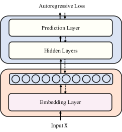
(a) Standard SRS

(b) AutoSAM

Figure 2. (a) is the architecture of the standard sequential recommender system (SRS). (b) is our proposed AutoSAM which augments the traditional sequential recommendation architecture with an additional sampler layer to adaptively explore the skew distribution of raw input. The dashed lines represent gradient backpropagation.

2. Related Work

2.1. Sequential Recommendation

Sequential recommendation aims to predict users’ future behaviors given their historical interaction data. Early approaches mainly fuse Markov Chain and matrix factorization to capture both long-term preferences and short- term item-item transitions (Rendle et al., 2010). Latter, with the success of neural network, recurrent neural network (RNN) methods are widely conducted in sequential recommendation (Hidasi et al., 2015, 2016). Besides, convolutional-based models (Tang and Wang, 2018; Yuan et al., 2019) can also be very effective in modeling sequential behaviors. In addition, we notice that graph neural networks (Wu et al., 2019; Xu et al., 2019) have become increasingly prevalent by constructing graph structures from session sequences. And in recent years, self-attention models (Kang and McAuley, 2018; Sun et al., 2019; de Souza Pereira Moreira et al., 2021) have shown their promising strengths in the capacity of long-term dependence modeling and easy parallel computation. Though successful, these methods mainly focus on the model architectures and treat all behaviors as uniformly positive, may lead to the sub-optimal performance.

2.2. Data-Centric Recommendation

As a data-driven technology, recommendation systems have attracted a series of works that consider from the data perspective in recent years (Qin et al., 2021; Xie et al., 2022a). To be specific, in SIM (Pi et al., 2020), a two-stage method with a general search unit(GSU) and an exact search unit is proposed to model long-term user behaviors better. Similarly, UBR4CTR (Qin et al., 2020) conducts retrieval-based method to achieve the goal. Besides, SDIM (Cao et al., 2022) proposed a sampling-based approach which samples similar items to the target by multiple hash functions. And some other works (Wang et al., 2021; Lin et al., 2023) mainly formulate a denoising task with the aims of filtering irrelevant or noise items. Despite effectiveness, these methods are mainly designed for CTR prediction, which may be not suitable to conduct the left-to-right generative loss and sample items dynamically in the SRS task. We also notice some works which attempt to capture more informative patterns between user behaviors sequence by designing advance model architectures. RETR (Yao et al., 2022) build recommender transformer for capturing the user behavior pathway. And an all-MLP based model is proposed (Zhou et al., 2022) which adopts Fourier transform with learnable filters to alleviate the influence of the noise item. Differently, in this paper, we present a general framework to learn the distributions of the raw inputs adaptively with carefully designed multi-objectives, so as to enhance the SRS with more informative and diverse training data.

3. Preliminaries

Before going into the details, we first introduce the research problem and revisit the sequential recommender systems.

3.1. Problem Definition

Assume that there are item set $\mathcal{I}=\{i_{1},i_{2},...,i_{|\mathcal{I}|}\}$ and user set $\mathcal{U}=\{u_{1},u_{2},...,u_{|\mathcal{U}|}\}$, we denote each behavior sequence of user $u\in\mathcal{U}$ as $X^{u}=[x_{1}^{u},x^{u}_{2},...,x_{n}^{u}]$, where $x_{t}^{u}\in\mathcal{I}$ is the item that $u$ interacted at step $t$ and $n$ is the sequence length. Sequential recommender systems (SRS) aim to predict the item that users might interact with at the next time step. Different from traditional SRS, the main idea behind this work is to sample historical behaviors with a policy $\pi(A^{u}|X^{u})$, where $A^{u}\in\{select=1,discard=0\}^{n}$, and then utilize $\hat{X^{u}}=[x_{k_{1}}^{u},x_{k_{2}}^{u},...,x_{k_{m}}^{u}]$ to train more generalizable SRS, in which $k$ is the set of time steps about sampled items, $m$ is the length of $\hat{X^{u}}$.

3.2. Sequential Recommender System

As shown in Figure 2(a), modern SRS mainly contain the components as following. First, each input item $x^{u}_{t}$ is mapped into an embedding vector by an embedding lookup operation. Then, the sequential embedding will be fed into stacked hidden layers in order to capture the long- and short-term dependence. Next, a prediction layer is adopted to generate the distribution of the user’s preferences at the next time step. Finally, to train the model, the auto-regressive generative loss are employed as optimization objectives, i.e., left-to-right supervision signals. Combining the cross-entropy loss with such an objective, the loss function can be written as follows:

(1) $$\mathcal{L}(X;\theta)=-\sum_{t=1}^{n-1}logP(y_{t}|X_{\leq t};\theta),$$

where $\theta$ denotes the parameters of the model, $y_{t}=x_{t+1}$ is the item expect to be predicted at step $t$, and $n$ is the input length.

4. AutoSAM: the Proposed Method

4.1. Overview of the Framework

The framework of our proposed AutoSAM is depicted in Figure 2(b). First, we employ a light-weighted sampler to adaptively learn the non-uniform distribution of the raw input, and then sample the informative sub-sets from the whole sequence. After that, the sequential recommender systems (SRS) are trained with these higher-quality and diverse samples to gain stronger generalizations. Considering the challenges of non-differentiable sampling actions and the necessity to introduce multiple decision factors, we further introduce a novel reinforcement learning based method to optimize the sampler. Specifically, we treat the sampler as the agent. For each time step $t$ of the user behavior sequence $X$, the sampler takes $X_{\leq t}$ as the current state $s_{t}$, and outputs an action $a_{t}\in\{0,1\}$ of the $t$-th item. Then, it observes the carefully designed multi-objective rewards from the environment to update the model via the policy gradient. Finally, the sampler could make optimal decisions by continuously interacting with the environment.

4.2. Sampler

We first transform sequence $X$ into embedding $E_{X}=\zeta_{X}+P_{X}$, where $\zeta$ and $P$ are the embedding matrix and position embedding, respectively. We suggest that the sample decisions should be based on both local and global information. Hence, the sampler leverages a Transformer Block with triangular mask matrix to aggregate the global information $X_{\leq t}$ at each step $t$, and then concatenate it with the local item embedding to generate the sample policy $\pi$ through an MLP layer. After that, binary decisions $A\in\{0,1\}^{n}$ are sampled from the Bernoulli distribution. The above procedure can be formulated as follows:

(2) $$H =Transformer(E)$$

$$\pi =Softmax(MLP([H,E])/\tau)\in\mathbb{R}^{n\times 2}$$

$$A \sim\pi\in\{0,1\}^{n},$$

where $\tau$ is the temperature of Softmax. Finally, we can build the sampled sub-set as $\hat{X}=\{x_{t}|a_{t}=1\}$.

4.3. Multi-Objective Rewards

Now we discuss how to design our reward, which plays an important role in learning the optimal $\pi$. As mentioned before, traditional SRS often follow the next item prediction task, which can neither update sampler network directly due to the non-differentiable challenge of discrete actions nor control the sample rate. In addition, such single objective may be too strict and one-sided. We argue that the proper decisions should not only focus on the target item but also consider the coherence with preceding context. Along this line, in this paper, we incorporate the major factors into the reward estimation, including Future Prediction and Sequence Perplexity.

4.3.1. Future Prediction

Generally, items that contribute to predicting the future interactions should be of more opportunities to be selected. To this end, we theoretically propose our rewards with consideration of the recommendation loss in Eq. 1. Since we train the SRS with the sampled sub-set $\hat{X}$, the objective can be written as follows:

(3) $$min\;J(\theta,\phi) =min\;\mathbb{E}_{X}\mathbb{E}_{A\sim\pi_{\phi}(A|X)}\big{[}\mathcal{L}(\hat{X};\theta)],$$

where $\theta$ and $\phi$ are the parameters of SRS and sampler, respectively, while sharing the embedding layer. To optimize this objective, we first transform the prediction loss to an equivalent form:

(4) $$\mathcal{L}(\hat{X};\theta) =\sum_{t=1}^{m-1}-logP(\hat{y}_{t}|\hat{X}_{\leq t};\theta)$$

$$=\sum_{t=1}^{n-1}-a_{t+1}logP(y_{t}|\{x_{k_{j}}|1\leq j\leq m-1;k_{j}\leq t\};\theta)$$

$$=\sum_{t=1}^{n-1}\mathcal{L}_{t}(X,A;\theta),$$

and then derive the gradients with respect to $\phi$:

(5) $$\nabla_{\phi}J(\theta,\phi) =\mathbb{E}_{X}\nabla_{\phi}\sum_{A}\pi_{\phi}(A|X)\mathcal{L}(\hat{X};\theta)$$

$$=\mathbb{E}_{X}\sum_{A}\pi_{\phi}(A|X)\nabla_{\phi}log\pi_{\phi}(A|X)\mathcal{L}(\hat{X};\theta)$$

$$=\mathbb{E}_{X}\mathbb{E}_{A\sim\pi_{\phi}(A|X)}\nabla_{\phi}\sum_{t=1}^{n}log\pi_{\phi}(a_{t}|X)\sum_{t=1}^{n-1}\mathcal{L}_{t}(X,A;\theta)$$

$$=\mathbb{E}_{X}\mathbb{E}_{A\sim\pi_{\phi}(A|X)}\nabla_{\phi}\sum_{t=1}^{n}-log\pi_{\phi}(a_{t}|X)r^{pre},$$

where $r^{pre}=\sum_{t=1}^{n-1}-\mathcal{L}_{t}(X,A;\theta)$ means the rewards associated to the sampler. In practice, we may make a few changes to it. First, we add a baseline $\mathcal{L}^{b}$ computed on raw input to $\mathcal{L}$ as it is always positive. Second, we discount the future rewards by a factor $\gamma\in[0,1]$ and ignore the targets whose sample probabilities are lower than $\psi$ to increase stability. Then, the future prediction reward at each time step $t$ can be defined as follows:

(6) $$r^{pre}_{t}=\sum_{t^{\prime}=t}^{n-1}-\gamma^{t^{\prime}-t}I[\pi_{\phi}(a_{t^{\prime}+1}|X)>\psi](\mathcal{L}_{t^{\prime}}(X,A;\theta)-\mathcal{L}_{t^{\prime}}^{b}),$$

in which $I[\cdot]$ is the indicator function, $\gamma$ is set to $0.9$ across all the experiments.

4.3.2. Sequence Perplexity

In addition to sampling based on future predictions, it should also be attached great importance to considering the coherence with previous context. Inspired by perplexity(PP), which is widely used to evaluate the quality of sentences in Natural Language Processing(NLP) (Liu et al., 2016; Dathathri et al., 2019) with the definition as follows:

(7) $$PP(X)=P(x_{1},x_{2},...x_{n})^{-\frac{1}{n}}=\prod_{t=1}^{n}P(x_{t}|X_{<t})^{-\frac{1}{n}}.$$

As words causing high perplexity tend to stray from the context, similarly, we insist that the items causing high perplexity may lack representativeness. A natural idea is to assign lower sampling probabilities to the items whose predicted probabilities according to historical behaviors are lower than $1/PP(X)$, so as to reduce the perplexity and obtain informative sub-sets in some way. To this end, the sampler should be encouraged to drop $x_{t}$ ($a_{t}=0$) while $P(x_{t}|X_{<t})<1/PP(X)$, and select $x_{t}$ while $P(x_{t}|X_{<t})>1/PP(X)$.

Note that the perplexity can be transformed to cross-entropy, in practice, we employ the SRS to compute the approximate objective at each time step $t$. Besides, a relax factor is further conducted to control the strictness of the sampler. Above all, the reward can be defined as follow:

(8) $$r^{pp}_{t}=(logP(x_{t}|X_{<t})-log\frac{1}{PP(X)}+b)(2a_{t}-1),$$

where $b$ is the relax factor, by which we can indirectly control the global sampling ratio. Generally, the smaller $b$ will lead the sampler to be stricter.

Algorithm 1 Learning the AutoSAM framework

1:  Initial SRS parameters $\theta$ and sampler parameters $\phi$.

2:  for $Epoch=1,2,...T$ do

3:     for $u=1,2,...|U|$ do

4:        $X\leftarrow[x_{1}^{u},x_{2}^{u},...,x_{n}^{u}]$;

5:        $\hat{X}\leftarrow[\;]$;

6:        Compute the policy $\pi_{\phi}(A|X)\in[0,1]^{n\times 2}$ by sampler;

7:        for $t=1,2,...n$ do

8:           Sample $a_{t}$ from $\pi_{t}$;

9:           if $a_{t}=1$ then

10:              Append $x_{t}$ to $\hat{X}$;

11:           end if

12:        end for

13:        Compute the recommendation loss $\mathcal{L}(\hat{X};\theta)$ according to Eq. 1;

14:        Compute overall sampling reward $r$ according to Eq. 6, 8;

15:        Update $\theta$ and $\phi$ according to Eq. 11;

16:     end for

17:  end for

In summary, our carefully designed rewards could solve the non-differentiable problem of discrete decisions, and guide the training of the sampler from multi-perspectives including future prediction and previous context. Besides, it is more flexible to control sample rate to balance effectiveness and efficiency in practice.

4.4. Optimization

We summarize the rewards with trade-off and scaling factors as:

(9) $$r=k(\lambda r^{pre}+(1-\lambda)r^{pp}).$$

To further learn the sequential recommendation task, we also derive the gradients according to Eq. 3 with respect to $\theta$:

(10) $$\nabla_{\theta}J(\theta,\phi)=\mathbb{E}_{X}\mathbb{E}_{A\sim\pi_{\phi}(A|X)}\nabla_{\theta}\mathcal{L}(\hat{X};\theta).$$

Finally, both the SRS and sampler can be optimized jointly in an end-to-end manner by combining the policy gradient:

(11) $$\theta \leftarrow\theta-\alpha_{1}\nabla_{\theta}\mathcal{L}(\hat{X};\theta)$$

$$\phi \leftarrow\phi+\alpha_{2}\nabla_{\phi}\sum_{t=1}^{n}log\pi_{\phi}(a_{t}|X)r_{t},$$

where $\alpha_{1}$, $\alpha_{2}$ are the learning rates of SRS and sampler respectively. Overall, we present our learning algorithm in Algorithm 1.

4.5. Time and Computation Complexity Analysis

To evaluate the efficiency of our proposed method for online services, we analyze the time complexity of AutoSAM during inference in this part. Similarly, we first sample representative historical behaviors, and then feed them to SRS for modeling the user sequence. Denote $L$ as the number of layers and $N$ as the sequence length. Since we conduct Transformer-based SRS whose time complexity is $\mathcal{O}(LN^{2})$, the sampling processing takes $\mathcal{O}(N^{2})$ and the sequence modeling can be done within $\mathcal{O}(L(\mathbb{E}[(\sum_{i=1}^{N}a_{i})^{2}]))=\mathcal{O}(L(\mu^{2}N^{2}+N\sigma^{2}))$, in which $\mu\in\{0,1\}$ denotes the average sampling rate while $\sigma$ is the variance. Thus, AutoSAM could reduce the time complexity of about $\mathcal{O}((L-\mu^{2}L-1)N^{2})$. Moreover, since sampling can be regarded as a binary classification problem, we believe the model could be more efficient while maintaining comparable performance by adopting much lighter sampler like RNN or MLP. We will explore such effects in the future work.

5. Experiments

We conduct experiments to answer the following research questions (RQ): RQ-1: Does AutoSAM outperform the SOTA models? RQ-2: Is the proposed framework general useful for various backbones? RQ-3: Could AutoSAM learns more potential preferred items of users in the future? RQ-4: What is the influence of key hyper-parameters to efficiency and effectiveness? RQ-5: What are sampled from the historical behaviors?

5.1. Experimental Setup

5.1.1. Datasets

We conduct four real-world datasets from different online platforms including Tmall, Alipay, Yelp, and Amazon Book (abbreviated as Amazon). For Tmall, Alipay and Amazon datasets, We filter users who interact with no more than 10 items. As for Yelp, we filter users who interact with no more than 5 items. And we set a maximum sequence length of 100 for all datasets. The statics of these datasets after processing are summarized in Table 1.

Table 1. Statics of the used datasets in the experiments.

Datasets	#Num. Users	#Num. Items	#Num. Actions	#Actions/Item	#Actions/User
Tmall	424,170	969,426	22,010,938	22.71	51.89
Alipay	520,064	2,076,041	20,976,085	10.10	40.33
Yelp	221,397	147,376	3,523,285	23.91	15.91
Amazon	724,012	1,822,885	18,216,875	9.99	25.16

5.1.2. Compared Methods

We first compare our proposed method from data perspective with following approaches: (1) FullSAM trains with full historical behaviors. (2) FMLP-Rec (Zhou et al., 2022) conducts Fourier transform with learnable filters to alleviate the influence of noise. (3) RETR (Yao et al., 2022) builds recommender transformer for capturing the user behavior pathway. (4) SDIM (Cao et al., 2022) retrieves relevant historical items that are similar to the target item by multiple hash functions to model long-term preference. (5) RanSAM, (6) LastSAM, (7) PopSAM samples random, last or most popular historical behaviors with a fixed probability respectively. We adopt SASRec (Kang and McAuley, 2018) as the sequential recommender system for all sample-based methods due to its effectiveness (Xie et al., 2022b). Besides, We also compare the models with other architectures: (8) PopRec ranks items based on their popularity. (9) BPR-MF (Rendle et al., 2012) is a well-known matrix factorization-based method optimized by Bayesian personalized ranking loss. (10) FPMC (Rendle et al., 2010) combines matrix factorization with the Markov chain. (11) GRU4Rec (Hidasi et al., 2015) adopts GRU to model item sequences. (12) NextitNet (Yuan et al., 2019) is a CNN-based method to capture long-term and short-term interests. (13) BERT4Rec (Sun et al., 2019) utilizes a bidirectional self-attention network to model user sequence. (14) SR-GNN (Wu et al., 2019) applies GNN with attention network to model each session.

Table 2. Recommendation performance comparison of different models over four datasets. The best performance and the second best performance methods are indicated by bold and underlined fonts. “IMP” denotes the improvements of our method compared to the best baseline.

Method	Tmall				Alipay				Yelp				Amazon
	N@10	N@20	R@10	R@20	N@10	N@20	R@10	R@20	N@10	N@20	R@10	R@20	N@10	N@20	R@10	R@20
PopRec	0.0045	0.0053	0.0087	0.0118	0.0136	0.0143	0.0155	0.0182	0.0037	0.0048	0.0066	0.0111	0.0016	0.0018	0.0030	0.0038
BPR-MF	0.0217	0.0268	0.0402	0.0602	0.0129	0.0142	0.0181	0.0234	0.0173	0.0228	0.0343	0.0564	0.0116	0.0145	0.0212	0.0324
FPMC	0.0379	0.0452	0.0683	0.0971	0.0572	0.0632	0.0907	0.1144	0.0210	0.0273	0.0407	0.0657	0.0481	0.0520	0.0662	0.0817
GRU4Rec	0.0410	0.0503	0.0765	0.1135	0.0450	0.0518	0.0779	0.1050	0.0213	0.0276	0.0415	0.0666	0.0370	0.0421	0.0581	0.0783
NextitNet	0.0425	0.0510	0.0775	0.1115	0.0498	0.0568	0.0850	0.1124	0.0229	0.0295	0.0447	0.0711	0.0441	0.0493	0.0666	0.0863
BERT4Rec	0.0496	0.0595	0.0906	0.1301	0.0485	0.0551	0.0815	0.1078	0.0235	0.0305	0.0460	0.0739	0.0386	0.0441	0.0618	0.0840
SR-GNN	0.0359	0.0437	0.0664	0.0975	0.0401	0.0459	0.0681	0.0915	0.0199	0.0255	0.0383	0.0608	0.0312	0.0355	0.0485	0.0655
FullSAM	0.0515	0.0614	0.0927	0.1320	0.0617	0.0695	0.1037	0.1346	0.0245	0.0314	0.0473	0.0746	0.0470	0.0524	0.0718	0.0932
FMLP-Rec	0.0558	0.0665	0.1007	0.1431	0.0630	0.0709	0.1052	0.1362	0.0263	0.0337	0.0506	0.0798	0.0480	0.0535	0.0729	0.0949
RETR	0.0526	0.0624	0.0942	0.1332	0.0608	0.0688	0.1027	0.1346	0.0250	0.0318	0.0478	0.0751	0.0471	0.0525	0.0711	0.0926
SDIM	0.0527	0.0626	0.0939	0.1333	0.0585	0.0685	0.0991	0.1332	0.0241	0.0308	0.0464	0.0734	0.0464	0.0513	0.0701	0.0898
RanSAM	0.0532	0.0633	0.0961	0.1354	0.0633	0.0713	0.1061	0.1380	0.0246	0.0315	0.0475	0.0749	0.0482	0.0539	0.0740	0.0967
LastSAM	0.0502	0.0600	0.0904	0.1291	0.0599	0.0667	0.0993	0.1297	0.0234	0.0297	0.0445	0.0698	0.0446	0.0514	0.0696	0.0893
PopSAM	0.0522	0.0623	0.0945	0.1347	0.0590	0.0665	0.0995	0.1292	0.0246	0.0316	0.0474	0.0752	0.0442	0.0496	0.0681	0.0893
AutoSAM	0.0604	0.0717	0.1084	0.1528	0.0672	0.0753	0.1117	0.1437	0.0272	0.0347	0.0521	0.0817	0.0549	0.0610	0.0831	0.1074
IMP	8.24%	7.82%	7.65%	6.78%	6.16%	5.61%	5.28%	4.13%	3.42%	2.97%	2.96%	2.38%	11.39%	13.17%	12.30%	11.07%

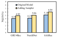
(a) N@10, Tmall

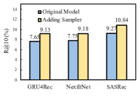
(b) R@10, Tmall

(c) N@10, Yelp

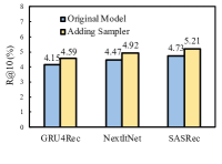
(d) R@10, Yelp

Figure 3. Performance comparison of different backbones enhanced by AutoSAM.

5.1.3. Hyper-parameter Settings

We set the batch size of 128 with 10, 000 random negative items per batch, and the embedding size is set to 128 for all methods. In all sampling based methods which employ two-layer SASRec as the backbone, we conduct 4 multi-head self-attention and 2 FFN layers, while the hidden size is set to 256. The sample rates of RanSAM, LastSAM and PopSAM are searched from $\{0.5,0.6,0.7,0.8,0.9\}$ We consistently employ Adam as the default optimizer for all recommenders, combined with a learning rate $\alpha_{1}$ of $1\times e^{-3}$. As for our sampler, we conduct SGD with a learning rate $\alpha_{2}$ of $1\times e^{-1}$. The remain parameters of baselines are carefully tuned or follow the default settings suggested by the original work. We use grid search to find the best group of AutoSAM’s hyper-parameters as shown in appendix.

5.1.4. Evaluation Metrics

We evaluate the recommendation performance over all candidate items with Recall and Normalized Discounted Cumulative Gain (NDCG). The first one is an evaluation of unranked retrieval sets while the other reflects the order of ranked lists. We consider top-k of overall item set for recommendations where $k\in\{10,20\}$ in our experiments. And we split the dataset into training, validation and testing sets following the leave-one-out strategy described in (Cheng et al., 2022; Zhao et al., 2022).

Table 3. Ablation study of each reward component, scaling factors $k$ and trade-off parameter $\lambda$.

Method	N@10	R@10	$k$	N@10	R@10	$\lambda$	N@10	R@10
AutoSAM	0.0672	0.1117	2e-1	0.0663	0.1111	0.00	0.0663	0.1109
w/o $r^{pre}$	0.0663	0.1109	2e-2	0.0666	0.1113	0.25	0.0668	0.1115
w/o $r^{pp}$	0.0603	0.1016	2e-3	0.0672	0.1117	0.50	0.0672	0.1117
w/o $r$	0.0581	0.0984	2e-4	0.0664	0.1109	0.75	0.0634	0.1057
			2e-5	0.0596	0.0995	1.00	0.0603	0.1016

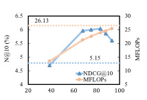
(a) Tmall

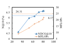
(b) Alipay

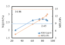
(c) Yelp

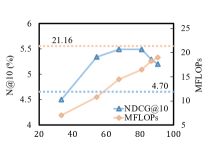
(d) Amazon

Figure 4. Performance and computation cost w.r.t. sample rates (portion of the kept items). The dashed line represents the baseline model, i.e., FullSAM.

5.2. Performance Comparison

The result of different models on datasets are shown in Table 2, from which the following observations confirm the answer of RQ-1. First of all, we can find that considering from the data perspective instead of treating all items as uniformly positive can benefit the performance. However, SDIM achieves limited improvement compared to FullSAM. A possible reason is that SDIM samples according to the target maybe too strict to capture the user’s rich interests. Besides, FMLP-Rec achieves much better performance than traditional SRS probably due to its stronger ability to filter noise information. And we surprisingly find that RanSAM outperforms FullSAM, this suggests that sampling can be regarded as a method of data augmentation in some way since different samples of each user are generated in different iteration rounds, which lead to significant enhancement in generalization capability by increasing the diversity of the training data. Unfortunately, RanSAM treats each interaction uniformly and may also drop lots of high-quality behaviors, making the improvement limited. Different from these baselines, the proposed AutoSAM adaptively explore the skew distribution of the raw input, and then enhance the sequntial recommender with informative samples. Consequently, our method performs best on all datasets, which gains an average improvement over the best baseline of 7.05%, 7.30% on Recall@10, NDCG@10, and 6.09%, 7.39% on Recall@20, NDCG@20 respectively.

5.3. Generality Analysis

In this part, we answer the RQ-2 by investigating the general applicability of AutoSAM to other sequential recommendation models. We conduct a performance comparison between models with and without the sampler on three different architectures: RNN-based GRU4Rec (Hidasi et al., 2015), CNN-based NextItNet (Yuan et al., 2019) and Transformer-based SASRec (Kang and McAuley, 2018). Figure 3 presents the comparison results in terms of test Recall and NDCG on Yelp and Tmall datasets. It is evident that all the sequential recommenders demonstrate significant improvements through the integration of automatic sampling, highlighting the generality of our AutoSAM for different backbones.

5.4. Evaluation of Compared Methods w.r.t. Number of Test Items

Traditional SRS often treat the item of the next step as the unique prediction target during training and evaluation, which may limit capturing the user’s rich interests. Actually, behaviors after multiple steps may also be in line with the user’s current preferences. Luckily, such a dilemma can be largely alleviated by the proposed AutoSAM. When $x_{t}$ is selected, the distribution of the prediction target at step $t$ satisfies that: $p(y_{t}=x_{t+n})=p(a_{t+n}=1)\prod_{i=t+1}^{t+n-1}p(a_{i}=0),$ which adaptively broadens the learning horizon and makes it possible to explore potential preferred items in the future. To verify such effect, we test the robustness of longer prediction to confirm the answer of RQ-3 by extending the test set with multiple time steps. Specifically, we re-split the datasets using time step where 1-st to ($n$-10)-th for training, ($n$-10+1)-th to ($n$-10+$i$)-th and ($n$-5+1)-th to ($n$-5+$i$)-th for validation and testing respectively, in which $i\in\{1,2,3,4,5\}$ denotes the number of items in test set. Performance w.r.t. the number of test items on the Tmall and Amazon datasets is shown in Table 4. The improvement over baseline substantially increases when more items in the future are added to the test set. This observation implies that AutoSAM releases the model from the constraint of always taking the next step as the target in traditional SRS, making the model more robust.

Table 4. Recommendation performance(Recall@10) comparison w.r.t. the number of test steps.

Dataset	Method	Num. of Test Steps
		1	2	3	4	5
Tmall	SASRec	7.99	7.13	6.52	6.09	5.78
	AutoSAM	9.10	8.15	7.51	7.04	6.67
	IMP	13.89%	14.31%	15.18%	15.60%	15.40%
Amazon	SASRec	8.22	6.18	5.00	4.20	3.57
	AutoSAM	9.01	7.04	5.80	4.90	4.18
	IMP	9.61%	13.92%	16.00%	16.67%	17.09%

5.5. Ablation Study

5.5.1. Effectiveness of Each Reward Component

In the left column of Tabel 3, we analyze the efficacy of each component of the reward on the Alipay dataset. From the results, we can find that removing either of the components decreases the performance. Besides, $r^{pp}$ plays a more important role than $r^{pre}$. A possible reason is that context coherence is more targeted at a single item which could more directly reflect its importance and representative. We further show the impact of scaling factor $k$ and trade-off parameter $\lambda$ by performing a grid search from {$2e^{-1}$, $2e^{-2}$, $2e^{-3}$, $2e^{-4}$,$2e^{-5}$} and $\{0,0.25,0.5,0.75,1\}$, respectively. The model achieves the best performance at $(k,\lambda)=(2e^{-3},0.5)$. The results demonstrate the effectiveness of the incorporation of these two aspects, and it also exhibits the stability of AutoSAM while the different settings of $k$ within the appropriate range bring few influence.

5.5.2. Efficiency and Effectiveness of Different Relax Factors

In practice, it is necessary to balance efficiency and effectiveness when adapting to online services in different scenarios. Thus, we control the relax factors $b$ in Eq. 8 to solve this problem and answer RQ-4. The performance and the computation cost of the well-trained recommender in inference w.r.t. average sample rate by setting relax factor from $\{-0.5,0,...2\}$ are shown in Figure 4. Note that the computation cost is measured with million floating-point operations (MFLOPs). We surprisingly observe that even preserving 50% interactions can achieve the comparable performance as baseline. However, while the sample rate reaches 80%, the performance becomes to drop which probably because the tolerant sampler leads to a uniform distribution. Besides, the shortened sequences save lots computations especially with small $b$. Since the sampling can be regarded as a binary classification problem which is much simpler than recommendation and requires only one layer, we believe AutoSAM could be more efficient than using full sequence as the model gets deeper.

5.6. Sample Analysis

5.6.1. Sampling Quality Evaluation.

Sampling decisions play important roles to the recommend performance while directly affecting the inputs of recommendation models (Ding et al., 2020; Zhang et al., 2021). Next, to answer RQ-5, we evaluate the sample qualities by comparing the portion of different kind behaviors on sampled and dropped items. Commonly, items that are purchased or added to favorites should be of more importance than clicked ones. Note that we do not use this kind of information during the training procedure. As shown in Figure 6, the proportion of purchases among picked items is higher than that among dropped items. According to this, we can find that the learned distributions are more significant to the user’s preference, which demonstrates the effectiveness of the sampler and also implies the necessity of treating behaviors non-uniformly. As it still keeps lots of clicked interactions, a possible reason is that the click items can also reflect the user’s interests to a great extent, and the factors behind that are usually very complex in the real world.

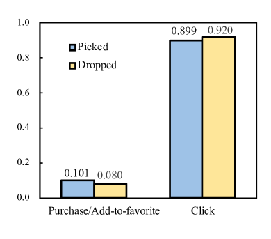
(a) Tmall

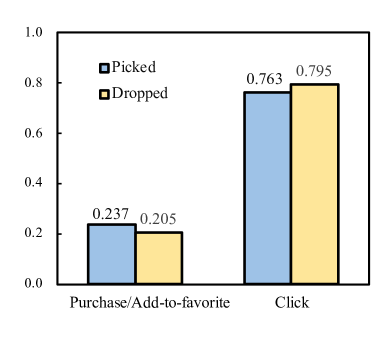
(b) Alipay

Figure 5. Portion of different kind behaviors of picked and dropped interactions.

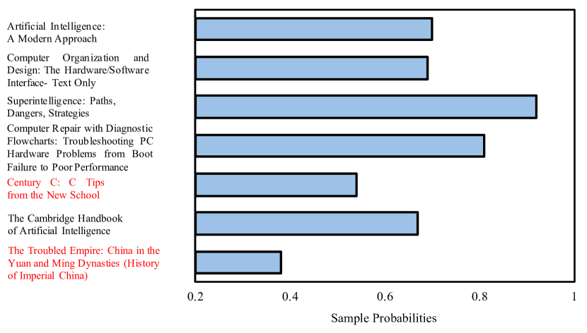
Figure 6. Case study analysis in terms of sampling distribution on Amazon Dataset.

5.6.2. Case Study

We additionally show several interesting case stduies in terms of sample probabilities on Amazon dataset in this part. Given historical behaviors, possibilities of being selected by sampler are partially shown with their titles in Figure 6. The case (a) is mainly about computer science while the case (b) is mainly about cooking. As we can see, items close to the global interests are more representative, naturally should of more chance to be selected. On the contrary, items in red seem to be irrelevant, resulting in fewer opportunities to be chosen. Such visualization also implies the importance of modeling the distributions of positive user behaviors instead of treating them as uniformly positive.

6. Conclusion

In this work, we proposed a general automatic sampling framework, named AutoSAM, to non-uniformly treat historical behaviors. Specifically, a light-weighted sampler was first leveraged to adaptively explore the distribution of raw input, so that the sequential recommender systems (SRS) could be trained with more informative and diverse samples. Considering the challenges of non-differentiable actions and the necessity to introduce multiple decision factors for sampling, we further introduced a novel reinforcement learning-based method to guide the training of the sampler. We carefully designed multi-objective rewards and combined policy gradient to optimize the whole framework in an end-to-end manner. We conducted extensive experiments on four public datasets. The experimental results showed that the AutoSAM could obtain a higher performance gain by adaptively sampling informative items, and also demonstrated the effectiveness of the sampler. We also noticed some limitations. AutoSAM conducts a transformer-based sampler, which may not be more efficient than baseline in the shallow SRS, according to Section 3.5. We believe this could be improved by adopting much lighter samplers like RNN or MLP, and will study this effect in the future. We hope this paper could inspire more works to be proposed from the data perspective for SRS.

Appendix A Implementation Details

A.1. Running Environment

The experiments are conducted on NVIDIA Telsa A100-40GB. Our proposed AutoSAM is implemented in Pytorch and Python 3.8.

A.2. Optimal Hyper-parameter

Table 5. AutoSAM’s hyper-parameter exploration in experiments.

Hyper-parameter	Tuning Range	Tmall	Alipay	Yelp	Amazon
$t$	$[1.0,3.0,5.0,7.0,9.0]$	5.0	5.0	5.0	3.0
$b$	$[-0.5,0.0,0.5,1.0,1.5,2.0]$	1.0	2.0	1.0	0.5
$k$	$[2e^{-2},2e^{-3},2e^{-4}]$	$2e^{-3}$	$2e^{-3}$	$2e^{-2}$	$2e^{-3}$
$\lambda$	$[0.25,0.5,0.75]$	$0.5$	$0.5$	$0.5$	$0.5$
$\psi_{0}$	$[0.2,0.5,0.8]$	$0.8$	$0.8$	$0.8$	$0.5$

We use grid search to find the best group of AutoSAM’s hyper-parameters shown in 5. Note that we change the threshold $\psi$ according to the following schedule: $\psi=\psi_{0}+0.03(Epoch-1)$.

Appendix B Experiment Details

B.1. Error Analysis

Table 6. Repeat experiment results and the corresponding standard deviation.

Metrics	Tmall	Alipay	Yelp	Amazon
N@10	$0.0604\pm 0.0008$	$0.0672\pm 0.0016$	$0.0272\pm 0.0002$	$0.0549\pm 0.0004$
N@20	$0.0717\pm 0.0009$	$0.0753\pm 0.0016$	$0.0347\pm 0.0002$	$0.0610\pm 0.0003$
R@10	$0.1084\pm 0.0013$	$0.1117\pm 0.0024$	$0.0521\pm 0.0006$	$0.0831\pm 0.0008$
R@20	$0.1528\pm 0.0017$	$0.1437\pm 0.0025$	$0.0817\pm 0.0009$	$0.1074\pm 0.0009$

We repeat the experiments three times to evaluate the stability of our proposed AutoSAM. The average performance and the corresponding standard deviation are shown in Table 6. As the standard deviations are basically at a low level, it indicates the small fluctuations of our approaches. Such stability is mainly due to the proper setting of the key parameters including temperature and scaling factors, which effectively prevent the model from collapsing.

B.2. Ablation Study of Temperature

The temperature $\tau$ in the Softmax function of the sampler significantly influences the distribution of sample probabilities, consequently impacting the recommendation performance of the sequential recommender system. In this part, we analyze this impact by varying $\tau$ from $\{1,3,5,7,9\}$. As shown in Figure 7, we observe that AutoSAM achieves the best performance at $\tau=5$. Deviating from this value, either by choosing too large or too small $\tau$, leads to a decline in performance. A possible explanation is that smaller $\tau$ may cause convergence to local optima, while larger $\tau$ results in nearly uniform probability distributions.

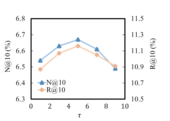
(a) Alipay

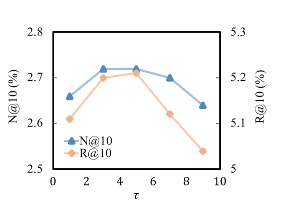
(b) Yelp

Figure 7. Ablation Study of temperature.

References

- (1)
- Cao et al. (2022) Yue Cao, Xiaojiang Zhou, Jiaqi Feng, Peihao Huang, Yao Xiao, Dayao Chen, and Sheng Chen. 2022. Sampling Is All You Need on Modeling Long-Term User Behaviors for CTR Prediction. In Proceedings of the 31st ACM International Conference on Information & Knowledge Management. 2974–2983.
- Cheng et al. (2022) Mingyue Cheng, Zhiding Liu, Qi Liu, Shenyang Ge, and Enhong Chen. 2022. Towards Automatic Discovering of Deep Hybrid Network Architecture for Sequential Recommendation. In Proceedings of the ACM Web Conference 2022. 1923–1932.
- Cheng et al. (2021) Mingyue Cheng, Fajie Yuan, Qi Liu, Shenyang Ge, Zhi Li, Runlong Yu, Defu Lian, Senchao Yuan, and Enhong Chen. 2021. Learning recommender systems with implicit feedback via soft target enhancement. In Proceedings of the 44th International ACM SIGIR Conference on Research and Development in Information Retrieval. 575–584.
- Dathathri et al. (2019) Sumanth Dathathri, Andrea Madotto, Janice Lan, Jane Hung, Eric Frank, Piero Molino, Jason Yosinski, and Rosanne Liu. 2019. Plug and play language models: A simple approach to controlled text generation. arXiv preprint arXiv:1912.02164 (2019).
- de Souza Pereira Moreira et al. (2021) Gabriel de Souza Pereira Moreira, Sara Rabhi, Jeong Min Lee, Ronay Ak, and Even Oldridge. 2021. Transformers4rec: Bridging the gap between nlp and sequential/session-based recommendation. In Proceedings of the 15th ACM Conference on Recommender Systems. 143–153.
- Ding et al. (2020) Jingtao Ding, Yuhan Quan, Quanming Yao, Yong Li, and Depeng Jin. 2020. Simplify and robustify negative sampling for implicit collaborative filtering. Advances in Neural Information Processing Systems 33 (2020), 1094–1105.
- Guo et al. (2017) Huifeng Guo, Ruiming Tang, Yunming Ye, Zhenguo Li, and Xiuqiang He. 2017. DeepFM: a factorization-machine based neural network for CTR prediction. arXiv preprint arXiv:1703.04247 (2017).
- He et al. (2023) Zhicheng He, Weiwen Liu, Wei Guo, Jiarui Qin, Yingxue Zhang, Yaochen Hu, and Ruiming Tang. 2023. A Survey on User Behavior Modeling in Recommender Systems. arXiv preprint arXiv:2302.11087 (2023).
- Hidasi et al. (2015) Balázs Hidasi, Alexandros Karatzoglou, Linas Baltrunas, and Domonkos Tikk. 2015. Session-based recommendations with recurrent neural networks. arXiv preprint arXiv:1511.06939 (2015).
- Hidasi et al. (2016) Balázs Hidasi, Massimo Quadrana, Alexandros Karatzoglou, and Domonkos Tikk. 2016. Parallel recurrent neural network architectures for feature-rich session-based recommendations. In Proceedings of the 10th ACM conference on recommender systems. 241–248.
- Huang et al. (2018) Jin Huang, Wayne Xin Zhao, Hongjian Dou, Ji-Rong Wen, and Edward Y Chang. 2018. Improving sequential recommendation with knowledge-enhanced memory networks. In The 41st international ACM SIGIR conference on research & development in information retrieval. 505–514.
- Huang et al. (2023) Zhenya Huang, Binbin Jin, Hongke Zhao, Qi Liu, Defu Lian, Bao Tengfei, and Enhong Chen. 2023. Personal or general? a hybrid strategy with multi-factors for news recommendation. ACM Transactions on Information Systems 41, 2 (2023), 1–29.
- Kang and McAuley (2018) Wang-Cheng Kang and Julian McAuley. 2018. Self-attentive sequential recommendation. In 2018 IEEE international conference on data mining (ICDM). IEEE, 197–206.
- Koren (2008) Yehuda Koren. 2008. Factorization meets the neighborhood: a multifaceted collaborative filtering model. In Proceedings of the 14th ACM SIGKDD international conference on Knowledge discovery and data mining. 426–434.
- Koren et al. (2009) Yehuda Koren, Robert Bell, and Chris Volinsky. 2009. Matrix factorization techniques for recommender systems. Computer 42, 8 (2009), 30–37.
- Li et al. (2017) Jing Li, Pengjie Ren, Zhumin Chen, Zhaochun Ren, Tao Lian, and Jun Ma. 2017. Neural attentive session-based recommendation. In Proceedings of the 2017 ACM on Conference on Information and Knowledge Management. 1419–1428.
- Lin et al. (2023) Weilin Lin, Xiangyu Zhao, Yejing Wang, Yuanshao Zhu, and Wanyu Wang. 2023. AutoDenoise: Automatic Data Instance Denoising for Recommendations. arXiv preprint arXiv:2303.06611 (2023).
- Liu et al. (2016) Chia-Wei Liu, Ryan Lowe, Iulian V Serban, Michael Noseworthy, Laurent Charlin, and Joelle Pineau. 2016. How not to evaluate your dialogue system: An empirical study of unsupervised evaluation metrics for dialogue response generation. arXiv preprint arXiv:1603.08023 (2016).
- Liu et al. (2018) Qi Liu, Hong-Ke Zhao, Le Wu, Zhi Li, and En-Hong Chen. 2018. Illuminating recommendation by understanding the explicit item relations. Journal of Computer Science and Technology 33 (2018), 739–755.
- Liu et al. (2022) Zhiding Liu, Mingyue Cheng, Qi Liu, Enhong Chen, et al. 2022. One Person, One Model–Learning Compound Router for Sequential Recommendation. arXiv preprint arXiv:2211.02824 (2022).
- Pi et al. (2020) Qi Pi, Guorui Zhou, Yujing Zhang, Zhe Wang, Lejian Ren, Ying Fan, Xiaoqiang Zhu, and Kun Gai. 2020. Search-based user interest modeling with lifelong sequential behavior data for click-through rate prediction. In Proceedings of the 29th ACM International Conference on Information & Knowledge Management. 2685–2692.
- Qin et al. (2023) Jiarui Qin, Weinan Zhang, Rong Su, Zhirong Liu, Weiwen Liu, Guangpeng Zhao, Hao Li, Ruiming Tang, Xiuqiang He, and Yong Yu. 2023. Learning to Retrieve User Behaviors for Click-Through Rate Estimation. ACM Transactions on Information Systems (2023).
- Qin et al. (2020) Jiarui Qin, Weinan Zhang, Xin Wu, Jiarui Jin, Yuchen Fang, and Yong Yu. 2020. User behavior retrieval for click-through rate prediction. In Proceedings of the 43rd International ACM SIGIR Conference on Research and Development in Information Retrieval. 2347–2356.
- Qin et al. (2021) Yuqi Qin, Pengfei Wang, and Chenliang Li. 2021. The world is binary: Contrastive learning for denoising next basket recommendation. In Proceedings of the 44th international ACM SIGIR conference on research and development in information retrieval. 859–868.
- Rendle et al. (2012) Steffen Rendle, Christoph Freudenthaler, Zeno Gantner, and Lars Schmidt-Thieme. 2012. BPR: Bayesian personalized ranking from implicit feedback. arXiv preprint arXiv:1205.2618 (2012).
- Rendle et al. (2010) Steffen Rendle, Christoph Freudenthaler, and Lars Schmidt-Thieme. 2010. Factorizing personalized markov chains for next-basket recommendation. In Proceedings of the 19th international conference on World wide web. 811–820.
- Singer et al. (2022) Uriel Singer, Haggai Roitman, Yotam Eshel, Alexander Nus, Ido Guy, Or Levi, Idan Hasson, and Eliyahu Kiperwasser. 2022. Sequential modeling with multiple attributes for watchlist recommendation in e-commerce. In Proceedings of the Fifteenth ACM International Conference on Web Search and Data Mining. 937–946.
- Sun et al. (2019) Fei Sun, Jun Liu, Jian Wu, Changhua Pei, Xiao Lin, Wenwu Ou, and Peng Jiang. 2019. BERT4Rec: Sequential recommendation with bidirectional encoder representations from transformer. In Proceedings of the 28th ACM international conference on information and knowledge management. 1441–1450.
- Tang and Wang (2018) Jiaxi Tang and Ke Wang. 2018. Personalized top-n sequential recommendation via convolutional sequence embedding. In Proceedings of the eleventh ACM international conference on web search and data mining. 565–573.
- Wang et al. (2017) Ruoxi Wang, Bin Fu, Gang Fu, and Mingliang Wang. 2017. Deep & cross network for ad click predictions. In Proceedings of the ADKDD’17. 1–7.
- Wang et al. (2019) Shoujin Wang, Liang Hu, Yan Wang, Longbing Cao, Quan Z Sheng, and Mehmet Orgun. 2019. Sequential recommender systems: challenges, progress and prospects. arXiv preprint arXiv:2001.04830 (2019).
- Wang et al. (2021) Wenjie Wang, Fuli Feng, Xiangnan He, Liqiang Nie, and Tat-Seng Chua. 2021. Denoising implicit feedback for recommendation. In Proceedings of the 14th ACM international conference on web search and data mining. 373–381.
- Wu et al. (2022) Le Wu, Xiangnan He, Xiang Wang, Kun Zhang, and Meng Wang. 2022. A survey on accuracy-oriented neural recommendation: From collaborative filtering to information-rich recommendation. IEEE Transactions on Knowledge and Data Engineering (2022).
- Wu et al. (2019) Shu Wu, Yuyuan Tang, Yanqiao Zhu, Liang Wang, Xing Xie, and Tieniu Tan. 2019. Session-based recommendation with graph neural networks. In Proceedings of the AAAI conference on artificial intelligence, Vol. 33. 346–353.
- Xie et al. (2022a) Ruobing Xie, Qi Liu, Liangdong Wang, Shukai Liu, Bo Zhang, and Leyu Lin. 2022a. Contrastive cross-domain recommendation in matching. In Proceedings of the 28th ACM SIGKDD Conference on Knowledge Discovery and Data Mining. 4226–4236.
- Xie et al. (2022b) Xu Xie, Fei Sun, Zhaoyang Liu, Shiwen Wu, Jinyang Gao, Jiandong Zhang, Bolin Ding, and Bin Cui. 2022b. Contrastive learning for sequential recommendation. In 2022 IEEE 38th international conference on data engineering (ICDE). IEEE, 1259–1273.
- Xu et al. (2019) Chengfeng Xu, Pengpeng Zhao, Yanchi Liu, Victor S Sheng, Jiajie Xu, Fuzhen Zhuang, Junhua Fang, and Xiaofang Zhou. 2019. Graph contextualized self-attention network for session-based recommendation.. In IJCAI, Vol. 19. 3940–3946.
- Yao et al. (2022) Zhiyu Yao, Xinyang Chen, Sinan Wang, Qinyan Dai, Yumeng Li, Tanchao Zhu, and Mingsheng Long. 2022. Recommender Transformers with Behavior Pathways. arXiv preprint arXiv:2206.06804 (2022).
- Yuan et al. (2019) Fajie Yuan, Alexandros Karatzoglou, Ioannis Arapakis, Joemon M Jose, and Xiangnan He. 2019. A simple convolutional generative network for next item recommendation. In Proceedings of the twelfth ACM international conference on web search and data mining. 582–590.
- Zhang et al. (2021) Yongqi Zhang, Quanming Yao, and Lei Chen. 2021. Simple and automated negative sampling for knowledge graph embedding. The VLDB Journal 30, 2 (2021), 259–285.
- Zhao et al. (2022) Wayne Xin Zhao, Zihan Lin, Zhichao Feng, Pengfei Wang, and Ji-Rong Wen. 2022. A revisiting study of appropriate offline evaluation for top-N recommendation algorithms. ACM Transactions on Information Systems 41, 2 (2022), 1–41.
- Zhou et al. (2022) Kun Zhou, Hui Yu, Wayne Xin Zhao, and Ji-Rong Wen. 2022. Filter-enhanced MLP is all you need for sequential recommendation. In Proceedings of the ACM Web Conference 2022. 2388–2399.