Analysis for satellite-based high-dimensional extended B92 and high-dimensional BB84 quantum key distribution
Abstract
A systematic analysis of the advantages and challenges associated with the satellite-based implementation of the high dimensional extended B92 (HD-Ext-B92) and high-dimensional BB84 (HD-BB84) protocol is analyzed. The method used earlier for obtaining the key rate for the HD-Ext-B92 is modified here and subsequently the variations of the key rate, probability distribution of key rate (PDR), and quantum bit error rate (QBER) with respect to dimension and noise parameter of a depolarizing channel is studied using the modified key rate equation. Further, the variations of average key rate (per pulse) with zenith angle and link length in different weather conditions in day and night considering extremely low noise for dimension are investigated using elliptic beam approximation. The effectiveness of the HD-(extended) protocols used here in creating satellite-based quantum key distribution links (both up-link and down-link) is established by appropriately modeling the atmosphere and analyzing the variation of average key rates with the probability distribution of the transmittance (PDT). The analysis performed here has revealed that in higher dimensions, HD-BB84 outperforms HD-Ext-B92 in terms of both key rate and noise tolerance. However, HD-BB84 experiences a more pronounced saturation of QBER in high dimensions.
I introduction
In an information-centric society, safeguarding communications and data emerges as a fundamental necessity. This necessity spans various applications, including but not limited to financial transactions, upholding individual privacy, and preserving the integrity of vital components within the Internet of Things. Cutting-edge classical cryptosystems like Rivest-Shamir-Adleman (RSA) algorithm provide security that hinges on the computational complexity of a problem and associated assumptions about the computational power of the adversaries [1]. However, these assumptions can be compromised once large-scale quantum computers come into play [2]. The remedy for this challenge is provided by a relatively recent cryptographic concept known as quantum key distribution (QKD) [3, 4, 5, 6]. Its security remains unaffected by algorithmic or computational progressions [7]. QKD enables the creation of symmetric keys between remote entities or parties, ensuring a level of confidentiality that is inherently constrained by the fundamental laws of physics [8, 9]. The polarization of light (photons) is a degree of freedom that is often utilized to realize different schemes for QKD and other schemes for secure quantum communication [10, 11, 12, 13, 14, 15, 16, 17]. Drifting qubits encoded in photons have the potential to be distributed over a distance of at most a few hundred kilometers through optical fibers [18, 19, 20, 21]. To extend these distances further, the utilization of quantum repeaters has been proposed [22, 23], but quantum repeaters are not yet commercially available. Further, maintaining light polarization possesses practical difficulties in long-distance QKD protocols. In the case of QKD protocols based on optical fiber, the polarization state is susceptible to alterations caused by random fluctuations of birefringence in the optical fiber [24, 25]. Further, the diminishing signal strength and the interference from ambient noise experienced during QKD transmissions via optical fibers hinder the attainment of substantial key rates beyond networks of metropolitan proportions [26, 27]. An alternative solution involves the proper utilization of optical satellite links, which can potentially overcome the limitations on transmission distances encountered by ground-based photonic communication schemes [28, 29, 30]. When dealing with open space conditions, while polarization exhibits greater resilience against atmospheric turbulence, in the reference frame of the satellite, variation of polarization is observed due to the motion of the satellite. This introduces a negative impact [31, 32, 33], and it becomes crucial to address these polarization fluctuations issues in both free-space and fiber-based QKD systems [34, 35]. Traditional approaches for addressing this challenge encompass the utilization of active polarization tracking devices [36, 26, 37, 38, 39, 40]. An alternative approach through a proof-of-principle experiment was proposed in 2023 [41]. Here, quantum state tomography was used to determine the optimal measurement bases for a single party. Moreover, embedding quantum technology within space platforms offers an avenue for conducting fundamental experiments in physics [42, 43] and pioneering innovative concepts like quantum clock synchronization [44, 45, 46] and quantum metrology [47]. Although this endeavor presents significant technological challenges, a variety of experimental investigations [48, 49, 50, 51, 52, 53, 54, 55] alongside theoretical inquiries [29, 56] have showcased the feasibility of this approach. These studies have demonstrated the viability of this approach using state-of-the-art technology already in use on the ground and approved for space operations [57, 58]. In fact, over the last decade, numerous experiments in free-space conditions have been conducted to assess the practicality of QKD setups on mobile platforms, encompassing diverse vehicles like hot-air balloons [52], trucks [59], aircraft [53, 55], and drones [60]. Consequently, in what has been characterized as the quantum space race [61], multiple international research groups in countries like Canada, Japan, Singapore, Europe, and China have been actively participating and trying to establish stable space-based communication channels [27, 62]. Notably, these efforts have seen the successful launch of satellites with payloads capable of being used in quantum communication [63, 64, 65, 66, 67, 68, 69]. The advancement of quantum technology has been greatly influenced by the healthy competition among the researchers [70, 71, 72], driving notable progress in quantum nonlinear optics, entangled photon generation techniques, and single photon detection in recent years. Given these remarkable technological strides, it is imperative to reevaluate the enhanced performance aspects of QKD through typical free-space connections. This reevaluation particularly focuses on the considerable rise in secure key generation rates compared to earlier experiments [73, 74, 48, 75, 76] (see Figure 1 of Ref. [77]). While this analysis (refer to Figure 1 of Ref. [77]) does not incorporate field tests utilizing prepare-and-measure schemes, it is worth noting that both terrestrial [78, 79] and satellite-based [64, 80] studies have effectively demonstrated decoy-state key exchange across free-space links at high rates. Furthermore, entanglement-based QKD protocols eliminate the necessity to place trust in the source of the satellite in a dual down-link scenario. Motivated by these facts, in the present work we wish to investigate the effectiveness of two specific protocols for QKD for the long-distance free-space secure quantum communication to be implemented with the assistance of a satellite. Before we specifically mention the protocols selected here for the investigation, we would like to briefly mention the logical evolution of the relevant protocols that led to the protocols of our interest.
The first protocol for QKD was proposed by Bennett and Brassard in 1984 (BB84 protocol) [3]. From the introduction of the BB84 protocol, there has been a continuous progression in both theoretical and practical aspects of QKD [21, 81, 82]. Nonetheless, owing to the formidable challenges posed by the generation, maintenance, and manipulation of quantum resources using current technologies, there has been a concerted effort to formulate QKD protocols with more straightforward conceptual frameworks such that the protocols would require fewer quantum resources. For instance, the BB84 protocol itself involves four quantum states and two measurement bases. In 1992, Bennett introduced a notably simpler QKD protocol named B92, which relies solely on two non-orthogonal states and two measurement bases [83]. However, B92 exhibits a heightened susceptibility to noise in contrast to alternative protocols like BB84, as indicated in the original paper [83]. Subsequently, in 2009, Lucamarini et al. [84] introduced an extended version of B92 (Ext-B92), incorporating two extra non-informative states to more effectively constrain Eve’s information gain. BB84, B92, and Ext-B92 protocols and most of the other existing protocols for QKD utilize qubits, which are two-dimensional systems, as the means of communication between Alice and Bob. Nevertheless, there have been limited investigations concerning the susceptibility of qudit-based schemes (i.e., schemes utilizing key encoding on -level systems) to eavesdropping in the case of high dimensional systems. Initiatives are currently underway to establish and investigate qudit systems within laboratory settings [85, 86]. Quantum systems with dimensions higher than two have demonstrated numerous benefits and intriguing characteristics compared to protocols based on qubits (as briefly discussed in [87]). There have been several studies related to their continuous variable counterparts ([88] and references therein). Further, certain protocols have exhibited the ability to tolerate high levels of channel noise as the system dimension expands, as evidenced by various studies [89, 90, 91, 92]. Motivated by these facts, in this article, we assess the performance of the key rate under different scenarios for the HD-Ext-B92 and HD-BB84 protocols. We calculate the key rate of the HD-Ext-B92 scheme without the inclusion of extra independent variables, in contrast to the method outlined in Ref. [93], which is explained further in Appendix A. We utilize the channel transmission to evaluate our results, focusing on light propagation through atmospheric links using the elliptic-beam approximation originally presented by Vasylyev et al. [94, 95]. Additionally, we incorporate the generalized approach and varying weather conditions introduced in [96]. Specifically, we investigate the applications of these models in quantum communication using Low Earth Orbit (LEO) satellites. Here, it may be noted that the methodology proposed in [94, 95, 96] has a notable impact on the transmittance value, which is influenced by beam parameters and the diameter of the receiving aperture.
Before delving into our main text, it is important to state that a satellite-based link is of two distinct types: the up-link and the down-link. These links should not be considered symmetrical due to the crucial distinction in the order of signal beam traversal through the atmosphere and space. In the up-link scenario, the signal beam first encounters the atmosphere, where it is subject to the effects of turbulence and scattering particles. It then proceeds into the expanse of space over long distances, where beam broadening becomes the dominant factor affecting its characteristics. Conversely, in the down-link scenario, the beam travels through space first and then through the atmosphere. In this scenario, the primary factor influencing the signal beam’s journey through extended space is the pointing error. This contrast in the order of traversal results in unique requirements for the receiving equipment on the ground and in space [97, 96].
This work is organized as follows. In Section II, we provide a detailed overview of the underlying theory of the HD-Ext-B92 and HD-BB84 protocols, as well as a comprehensive examination of the impact of atmospheric conditions on satellite communication links and the elliptical approximation of beam deformation at the receiver. Appendix A is dedicated to the necessary calculations to derive the key rate for the HD-Ext-B92 protocol. In Section III, an extensive investigation is done on the performance of these two high-dimensional protocols with the help of the appropriate illustration of the results of the simulation. Finally, we summarize our paper with the findings being consolidated and deliberated upon in Section IV.
II Preliminaries: High-dimensional B92 and BB84 protocols and Elliptic beam approximation
Numerous researchers have extensively investigated the unconditional security of QKD-based protocols, and their research, (see for examples, [98, 99]) has consistently revealed increasingly robust results. For instance, in [99], a noise tolerance of 6.5% was reported for the B92 protocol. Depending on the user’s selected key encoding states, the noise tolerance for this B92 protocol can extend up to 11% in the asymptotic scenario, as demonstrated in [84]. This level of noise tolerance is comparable to that of BB84. In scenarios with a finite key length, as indicated in [100], the protocol still maintains a minimum noise tolerance of 7%. In this context, we summarize the key-rate analysis for HD-Ext-B92 and HD-BB84 protocols. We modify the calculation for HD-Ext-B92 using a theorem to eliminate any additional free parameters (as detailed in Appendix A). Additionally, we briefly delve into the methodology of elliptical beam approximation, designed to encompass satellite-based connections while accounting for signal losses in various real-world scenarios, including diverse weather conditions. This methodology is particularly tailored for application in LEO satellite contexts.
II.1 High-dimensional extended B92 protocol and high-dimensional BB84 protocol
II.1.1 HD-Ext-B92
Here, we summarize the HD-Ext-B92 protocol and recap some important steps involved in the parameter estimation process proposed in Ref. [93]. In fact, in this section, after briefly discussing the HD-Ext-B92 protocol we modify the derivation of the asymptotic key rate given in [93]. Before explaining the protocol, we would like to introduce the notations used and the methodology for achieving key rate. and are the fixed states and defined from d-dimensional computational basis states , and is a fixed state which is chosen from d-dimensional diagonal basis (-basis) states.
State preparation and transmission: Alice randomly chooses key-round and test-round. The key-round is employed for generating raw key bit and test-round is employed to estimate error for this protocol. Alice prepares a sequence with states and to encode classical bit values and in key-round, respectively, and sends it to Bob. The basis information is kept secret. If this is a test-round, she uniformly prepares the states , , or with random choice and sends the sequence to Bob keeping the basis information secret until he measures the sequence.
Measurement and classical announcement: In a key-round, after getting the sequence from Alice, Bob will measure each state of the received sequence either with basis or by a POVM bases defined by and referred to as POVM , where denotes d-dimensional identity operator. Bob sets the bit value as when he observes by using measurement basis , i.e., any measurement outcome in basis other than ; and he sets bit value when his measurement outcome using POVM is other than . All other results are not taken into account as conclusive measurements. Alice and Bob discard the iteration for inconclusive outcomes in key-round, and determine the channel error rate in test-round by announcing their basis choices and measurement results using an authenticated classical channel. Finally, they run the error correction and privacy amplification protocols to get the final secure key.
In their work [93], authors proposed a collective attack by Eve in which she can independently and identically attack each round of the protocol. Eve also can delay measurement on her register (quantum memory) after completion of the protocol. The Devetak Winter key rate equation [101, 102] is used to compute the key rate in the asymptotic limit111For instance, we are interested in seeing the performance of satellite-based communication in the infinitely generated raw key scenarios.:
| (1) |
this analysis helps us to obtain the minimum value of the key rate by subtracting conditional Shannon entropy from conditional von Neumann . Here, is defined as the entropy or the uncertainty present in Alice’s classical register given Eve’s quantum memory and denotes the entropy present in Alice’s register given Bob’s classical register . Here, is determined as a number of secret key bits over the transmission of number of raw key. In Eq. (1), elucidates the infimum value of key rate under all collective attacks performed by Eve. We apply a Theorem [103] and analyze the parameter estimation (see Ref. [93]) to derive and . By utilizing these findings we can determine the lower bound of key rate (see Appendix A).
II.1.2 HD-BB84
In a two-level system, BB84 [3] protocol is well studied both in theoretical and experimental domains. Essentially two-dimensional quantum states (qubits) are used to realize this scheme for QKD which uses two mutually unbiased bases randomly. In a more general scenario, higher dimensional systems (qudits) can be used to realize the same task (i.e., QKD), and such a modified version of BB84 protocol is referred to as qudit- (i.e., a quantum state in -dimensional Hilbert space) based BB84 protocol or HD-BB84 protocol. Here, we briefly discuss the HD-BB84 protocol [104] and the necessary formulae to compute the secret key rate. In this protocol, sender Bob sends a qudit sequence to the receiver Alice after preparing each qudit randomly in one of the possible states where the basis is also selected randomly between one of the two mutually complementary bases. Alice also applies measurement operation on the qudit by randomly choosing one of these two bases. Subsequently, they announce their bases choice in a public authenticated classical channel [104]) and obtain correlated -ary random variables when they use the same bases (considering noise-free quantum channel). With probability, Alice and Bob use different bases and yield uncorrelated results which are considered as discarded data after key-sifting sub-protocol. This method ensures that any effort made by an eavesdropper, Eve (who is unaware of the chosen basis), to obtain information about Bob’s state will result in an error in transmission, which can subsequently be detected by the legitimate parties.
To ensure a smooth comprehension of readers we would like to provide a concise overview of key points discussed in Ref. [105]. in Ref. [105], authors have modified the Maassen and Uffink bound [106, 107] to establish a new bound on the uncertainties associated with the measurement results, contingent on the amount of entanglement between the measured particle , and the quantum memory (. This relationship can be expressed mathematically as,
| (2) |
where, and are two possible observable like measurement bases and refers to the qudit measured by Alice which is sent by Bob and refers to the qudit which represents the quantum memory of Bob. represents von Neumann entropy and quantifies the amount of entanglement between and . , where and are the eigenvectors of and , respectively. Using a result established by Devetak and Winter [101], the minimum limit on the quantity of key that Alice and Bob can extract from each state can be expressed as 222Here, Z and X can be employed in a similar manner or with a similar effect.. This limit is applied when the eavesdropper is trying to obtain the key from the composite quantum system333Eve performs an entanglement operation using her ancillary state with Alice’s state () and Bob’s quantum memory (). , where is Alice’s particle, is Bob’s quantum memory, and is Eve’s ancillary state. Equation (2) may be reformulated as (see Supplementary Information of [105]), and the key rate equation may be written as . Since cannot exceed and using Fano’s inequality444Fano’s inequality: . , we can obtain
| (3) |
For the binary encoding and decoding scheme the conditional entropy of Alice’s measurement outcome given Bob’s measurement result is equal to , where is quantum bit error rate (QBER) [108, 109]. Here, is the depolarizing channel parameter i.e., the probability that outcome of the by Alice and Bob is not equal and is binary entropy.
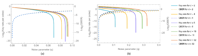
To analyze the behavior of the key rate per pulse and the QBER concerning the noise parameter in both the above-discussed HD protocols, we utilize the key rate equations (refer to Eqs. (1), (3), and Appendix A) and the binary QBER function . Now, we analyze the result illustrated in Figure 1 for HD-Ext-B92 and HD-BB84 schemes. We can observe in the HD-Ext-B92 protocol that events with mismatched bases are not disregarded, which occurs when Alice and Bob employ different measurement bases. These events can significantly enhance key generation rates [93, 110, 111, 112, 113], and therefore noise tolerance is also increased for this scheme which is evident from the graph. We plot the variation of the key rate of HD-Ext-B92 protocol with noise parameter () in a depolarizing channel in the -dimensional Hilbert space; we also depict the variation of QBER with the same noise parameter . It may be observed that as the value of increases, the tolerance for noise also increases, showing a rise from to . It is apt to note that, the maximum tolerable noise is dependent on the choice of both the depolarizing channel and of Eve’s ancilla state, since, these two factors significantly impact parameter estimation and consequently affect the key rate. Nevertheless, our analysis is confined to a specific choice of these two factors, which have been outlined in Appendix A. In Figure 1 (a), it becomes evident that the QBER remains constant across different values. The plots representing the distinct values (i.e., ) overlap in QBER analysis, indicating consistent outcomes for higher-dimensional cases of the HD-Ext-B92 protocol. Additionally, the graph (represented by a dotted line) demonstrates that the QBER reaches a saturation point for a particular value (for HD-Ext-B92). We have computed the initial point where the QBER begins to rise for various values and observed a physically reasonable variation. For instance, when is , the QBER is approximately . As the value increases to , the QBER saturates at approximately at . Now, we analyze the plots for HD-BB84 in Figure 1 (b) and undertake a comprehensive comparison with HD-Ext-B92. A numerical assessment reveals that the key rate increases as the value of rises for HD-BB84. Conversely, in HD-Ext-B92, the minimum key rate remains fairly consistent for all values which is around . Further, the noise tolerance is increased significantly with a greater value of in HD-BB84. For instance, the tolerable noise is for (for qubit) and with the increased value of , this limit increases to . This outcome demonstrates the advantage of opting for the HD-BB84 protocol over HD-Ext-B92 when considering aspects like key rate and noise tolerance. HD-BB84 surpasses the HD-Ext-B92 protocol. It is worth mentioning that in the original scheme of HD-Ext-B92 [93], authors do not employ two complete bases as HD-BB84 does. In their approach, they utilize a simplified version in which Alice’s requirement is reduced to transmitting just three states, and Bob only needs to carry out partial measurements within the second basis [93]. Additionally, it is important to highlight that they did not select an optimal basis configuration. Alternate choices for the encoding state might yield greater key rates for the HD-Ext-B92 protocol, as shown in cases involving qubits [84, 103]. If we examine the QBER aspect within the context of HD-BB84, it becomes apparent that the variation of QBER with the noise parameter () rapidly converges to a saturation value () as the dimension of qudit increases. In contrast to the HD-Ext-B92 protocol, the susceptibility of QBER to noise is notably more vulnerable in the HD-BB84 protocol. Moreover, as depicted in Figure 1, when considering , the saturation point of noise tolerance is attained in the HD-Ext-B92 protocol. In contrast, in the HD-BB84 protocol, the rate at which noise tolerance increases becomes progressively lower as increases. It is noteworthy that at , the QBER has not yet reached its saturation point (for HD-BB84); this point will be reached at higher values of .
II.2 Satellite-based optical links: model used for the elliptic beam approximation
In this article, we aim to analyze the performance of key rates in various situations of HD-Ext-B92 and HD-BB84 protocols. The channel transmission for the light propagation through atmospheric links using elliptic-beam approximation as introduced by Vasylyev et al. [94, 95] will be employed to perform the analysis. Further, in what follows, we impose the generalized approach555Using non-uniform link between a satellite and the ground station, referred to in Eq. (6). and different weather conditions as introduced in [96]. This method yields an impact on the value of transmittance as the transmittance is determined by beam parameters along with the diameter of the receiving aperture. To provide readers with a clearer understanding of both the elliptic beam approximation and its modified version in a more comprehensive manner, in this section, we offer a succinct explanation of the underlying theory.
Temporal and spatial fluctuations in temperature and pressure within turbulent atmospheric flows result in random variations of the air’s refractive index. Consequently, the atmosphere introduces losses to transmitted photons, which are detected at the receiver through a detection module featuring a limited aperture. The transmitted signal undergoes degradation due to phenomena like beam wandering, broadening, deformation, and similar effects. We can examine this scenario by focusing on a Gaussian beam propagating along the z axis, reaching the aperture plane positioned at a distance . The Gaussian beam is directed through a link that spans both the atmosphere and vacuum, originating from either a transmitter situated in orbit or a ground station. The link is characterized by non-uniform conditions. Generally, the varying intensity transmittance of such a signal (received beam) via a circular aperture of radius of the receiving telescope is expressed as follows [114, 94]:
| (4) |
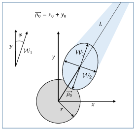
where represents the beam envelope at the receiver plane, located at a distance from the transmitter, and is the normalized intensity with respect to full plane, where denotes the position vector within the transverse plane. The vector parameter fully characterizes the state of the beam at the receiver plane (see Figure 2),
| (5) |
, , , and imply the beam centroid coordinates, the principal semi-axes of the elliptic beam profile, and the orientation angle of the elliptic beam, respectively. The transmittance is determined by these beam parameters along with the radius of the receiving aperture ().
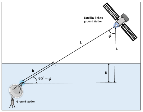
In general, the atmosphere can be categorized into distinct layers, each characterized by various physical parameters such as air density, pressure, temperature, the presence of ionized particles, and more. The arrangement of these layers varies according to location, particularly concerning the extent of each layer’s thickness. Without loss of generality, we adopt a simplified model of a satellite-based optical link [96]. This model entails a uniform atmosphere up to a specific altitude denoted as , beyond which a vacuum extends all the way to the satellite situated at an altitude marked as , as illustrated in Figure 3. Rather than dealing with a continuous range of values characterizing physical quantities as a function of altitude, this approach involves just two key parameters. These parameters encompass the value of the physical quantity within the uniform atmosphere and the effective altitude range, . This simplification is likely to be quite accurate because atmospheric influences are predominantly significant only within the initial to kilometers above the Earth’s surface. This is particularly relevant considering that the standard orbital height for LEO satellites is above 400 kilometers . In our analysis, we set the value of to km, and assume that the zenith angle falls within the range of . Under these conditions, the range of the satellite’s orbit suitable for key distribution is approximately km666The correlation between total link length and zenith angle is, .. The given context mandates that the effective atmospheric thickness remains constant at 20 km, by the aforementioned factors. We extend the discussion by maintaining the premise that the parameters quantifying the influence of atmospheric effects remain constant (with values greater than ) within the atmosphere and are set to outside it. In this context, we can make use of the assumption that,
| (6) |
Here, represents the refractive index structure constant777Several altitude-dependent models describing the refractive index structure constant have been documented [115, 116, 117, 118]. Among these, the parametric fit proposed by Hufnagel and Valley is widely adopted and faithfully captures the characteristics of in climates characteristic of mid-latitudes [116, 115]., and denotes the density of scattering particles [119, 120]. The function corresponds to the Heaviside step-function888The value of this function is zero for negative arguments and one for positive arguments. This function falls within the broader category of step functions.. As stated above, the parameter signifies the longitudinal coordinate, while stands for the overall length of the link. Additionally, represents the distance covered within the atmosphere, as illustrated in the accompanying Figure 3.
Now, let’s consider the transmittance, as defined in Eq. (4), for an elliptic beam that strikes a circular aperture with a radius of . This transmittance can be expressed as follows [94]:
| (7) |
In this context, represents the radius of the aperture, while and denote the polar coordinates of the vector ,
here, and represent polar coordinates corresponding to the vector ,
and
These expressions can be employed for numerical integration, as described in Eq. (7), through the Monte Carlo method or another effective technique for the same purpose. To simplify the process of integration using the Monte Carlo method, it requires the generation of sets of values for the vector (see Eq. (5)). It is assumed that the angle follows a uniform distribution over the interval and other parameters999To compute transmittance, first one has to evaluate from using relation Here, is the beam spot radius at the transmitter. () follow the normal distribution [121]. Substitution of the simulated values of into Eq. (7) makes it feasible to perform the numerical integration. The outcome of this process also involves the extinction factor101010The parameter denotes the extinction losses caused by atmospheric back-scattering and absorption. It varies depending on the elevation angle or zenith angle [97, 122]., , thereby producing atmospheric transmittance values, denoted as , where ranges from to . The necessary parameters for simulation are described in Appendix B which are calculated according to our model. These expressions are different for up-link and down-link configuration as different expressions mentioned in Eq. (6) are used for up-link and down-link configuration.
In the next section, we will evaluate the effectiveness of the HD protocols selected by us in the satellite-based links. To conduct this assessment, we need average key rates over the probability distribution of the transmittance (PDT)111111Some authors followed the relation with to represent the channel transmittance with the form of attenuation, here, total link length and is loss in the channel transmission . computed for different link lengths and configurations. The same can be expressed as [96],
| (8) |
where, represents the average key rate, while signifies the key rate corresponding to a specific transmittance value. The PDT is denoted as . To compute the integral average, the interval is divided into bins, each centered at for ranging from to , and is evaluated by combining the weighted sum of the rates. The estimation of relies on random sampling, as explained in the earlier paragraph. The formulations for the distinct implementations key rates can be found in Section II.1.
III Performance analysis of protocols after simulation
In this section, we elaborately analyze the impact of PDT121212See PDT in Figures 3 and 4 in Ref. [96] after random sampling of beam parameters for a down-link and an up-link, respectively. on key rate after the weighted sum, as well as the probability distribution of key rate (PDR) concerning the HD-Ext-B92 and HD-BB84 protocols. The minimum separation between Alice and Bob (i.e., altitude of the satellite) remains constant at a distance of km, as the primary focus is on scenarios involving LEO satellites like the Chinese satellite Micius [64, 68, 69, 63]. We present outcomes of numerical simulation for satellite-based HD-Ext-B92 and HD-BB84 schemes under asymptotic conditions. The simulation incorporates the experimental parameters outlined in Table 1 [123, 124, 96]. The crucial factors in this scenario include not only those associated with atmospheric influences but also the radii of the transmitting and receiving telescopes, along with the wavelength of the signal. For the satellite in orbit, we opted for a radius of cm (), while the ground station telescope has a radius of m, and the signal wavelength is nm. Based on Eq. (6), it is evident that a down-link pertains to satellite-to-ground communication, where atmospheric effects become significant only in the latter part of the propagation process, i.e., when exceeds . On the other hand, for up-links, these effects are relevant only when is below .
| Parameter | Value | Short description |
|---|---|---|
| 15 cm, 50 cm | Down-link, up-link | |
| 50 cm, 15 cm | Down-link, up-link | |
| 785 nm | Wavelength of the signal light | |
| 0.7 | Parameter in | |
| rad | Pointing error | |
| 20 km | Atmosphere thickness | |
| 500 km | Minimum altitude (at zenith) | |
| 0.61 | Night-time condition 1 | |
| 0.01 | Day-time condition 1 | |
| 3.00 | Night-time condition 2 | |
| 0.05 | Day-time condition 2 | |
| 6.10 | Night-time condition 3 | |
| 0.10 | Day-time condition 3 | |
| Night-time condition 1 | ||
| Day-time condition 1 | ||
| Night-time condition 2 | ||
| Day-time condition 2 | ||
| Night-time condition 3 | ||
| Day-time condition 3 |
From Appendix B, it becomes evident, as expected that the impact of atmospheric effects is considerably more pronounced in the case of up-links compared to down-links. The underlying phenomena at play here, namely beam deflection and broadening, encompass angular effects. These effects play a role in determining the ultimate size of the beam, thus influencing the channel losses. Their magnitude is directly proportional to the distance covered after the initiation of the effect known as kick in effect. For up-links, these effects manifest near the transmitter, resulting in beam broadening spanning hundreds of kilometers before detection at the satellite. Conversely, in the down-link scenario, the majority of the beam’s trajectory occurs within a vacuum, with atmospheric effects coming into play only during the final fifteen to twenty kilometers before reaching the receiver. A secondary distinction lies in the origin of fluctuations in the position of the beam centroid, denoted as . In up-links, the atmosphere-induced deflections tend to be significantly more influential than pointing errors (), which is disregarded. On the other hand, in down-links, the beam dimensions are already substantially larger than any turbulent irregularities at the top of the atmosphere. As a consequence, the resulting beam wandering due to atmospheric effects can be neglected, rendering pointing errors the dominant contributing factor.
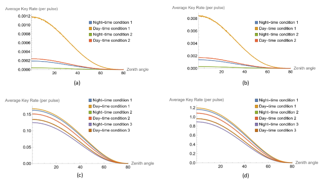
We aim to investigate the average key rate as a function of zenith angle, considering minimal noise. Figures 4 illustrate the average key rate using the PDT concerning the angle relative to the zenith. This analysis is carried out for both up-links and down-links across various weather conditions for dimension131313The weather data information is used from Ref. [96]. We also mention the required information in Table 1., (see Table 1). Each data point on the graph is derived from parameter samples in Eq. (5) and computed using Eq. (7). In Figures 4 (a) and 4 (b), the graphs reveal that during daytime condition 1, the highest average key rate is yielded in the zenith position ( and ) for HD-Ext-B92 and HD-BB84 protocols, respectively, in the up-link configuration. Notably, the key rate141414For ease of reference, we will refer to the average key rate as the "key rate". is slightly greater for HD-BB84 which corresponds to the expected result. For the same configuration, the key rate sharply diminishes under other conditions (Day 2 and Night 1-2). Comparatively, for HD-Ext-B92, the maximum value of the key rate () is nearly ten times lower than that of the HD-BB84 protocol () corresponding to the day condition 2. A similar comparison holds for night 1/2 conditions. For these conditions, the key rate becomes approximately zero at zenith angle . It may be noted that in night-time condition 1, the key rate is lower than in day-time condition 2 for both schemes within the same configuration. Based on these observations, we can infer that daytime transmission in the up-link configuration performs more favorably than nighttime transmission. Due to the very low key rate during night-time condition 2, we have chosen to negate condition 3, both in night-time and day-time, from the graphical representation. The down-link configuration is depicted in Figures 4 (c) and 4 (d). As previously discussed, the influence of atmospheric effects is comparatively reduced in the down-link configuration compared to the up-link configuration. Consequently, the performance of the link transmittance is superior for down-link as compared to up-link. This is supported by Figures 4 (c) and 4 (d), which further highlight the enhanced key rate. From these two figures, the overall plot patterns can be seen to be (sequential arrangement of plots representing different weather conditions) consistent for both protocols. The sequence of different weather conditions that yield higher key rate values follows this order: day-time condition 1, night-time condition 1, day-time condition 2, day-time condition 3, night-time condition 2, and night-time condition 3. Additionally, it can be seen that similar to the up-link scenario, the daytime conditions favor channel transmission over the nighttime conditions. This pattern remains consistent across both scenarios. Of particular interest is the comparison between operations during night-time and day-time. During daylight hours, higher temperatures facilitate stronger winds and heightened mixing across distinct atmospheric layers. This generates more prominent turbulence effects. However, on average, clear days witness a reduced moisture content in the lower atmosphere compared to night-time conditions. Consequently, the scattering of particles causes less pronounced beam spreading. Conversely, during night-time, the cooler temperatures result in an atmosphere with lower turbulence levels, coupled with the formation of mist and haze. In such circumstances, scattering tends to have a more substantial impact at night-time than the effects induced by turbulence at day-time. In the down-link scenario, during day-time condition 1, the highest achievable key rates are and for HD-Ext-B92 and HD-BB84 protocols, respectively. Conversely, in night-time condition 3, the highest attainable key rates are and . The key rate ratio, in the down-link scenario, between the HD-BB84 and HD-Ext-B92 protocols is for the maximum scenario and for the minimum scenario. This observation substantiates the anticipated outcome that HD-BB84 consistently outperforms HD-Ext-B92. Furthermore, the key rate decreases significantly within the zenith angle range of to for the down-link scenario, whereas for the up-link scenario, this reduction begins at a zenith angle of . Intuitively, down-link transmission exhibits a higher tolerance for larger zenith angles compared to up-link transmission.
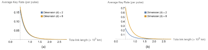
To obtain the best possible results, hereafter we focus on the down-link configuration under optimal weather conditions where the average key rate is highest (cf. Figure 4). Specifically, we analyze and illustrate the variation of key rate with total link length () in day-time condition 1 within down-link configuration, assuming an extremely low noise. In this scenario, the HD-Ext-B92 protocol yields maximum key rates of 0.17 and 0.155 for qudit dimensions 8 and 2, respectively, as illustrated in Figure 5 (a). Notably, the key rate of the HD-BB84 protocol exhibits notable fluctuations across different dimensions. As can be seen from Figure 5 (b), for qudit dimensions 8 and 2, the maximum key rates are 0.7 and 0.24, respectively. This is consistent with the results in Figure 4.
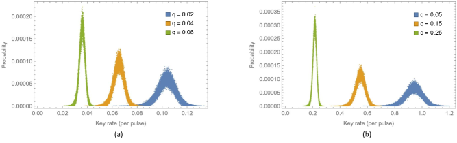
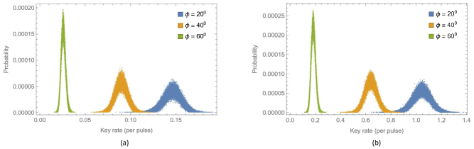
In Figure 6, we present the PDR with different values of noise parameter () at the zenith position () under down-link configuration. In this context, we employ the optimal performance scenario during day-time condition 1 utilizing qudit dimension of 32. We have used a data set of beam parameters to simulate the values of the average key rate and approximate the results to six (five) decimal places151515This is a good choice of approximation to represent, well-suited for PDR representation. to get PDR plots for HD-Ext-B92 (HD-BB84). Within the HD-Ext-B92 protocol, comparing the cases of and (in Figure 6 (a)), we observe a higher key rate for , while the maximum value of probability of key rate is greater for . The maximum values of probability are consistently greater with greater values of noise parameter. Notably, a higher key rate corresponds to a lower value of probability of occurrence. A specific shape of PDT (as is the case here) implies that the shape of the PDR would remain the same with different noise parameters and different zenith angles (or equivalently with different distances). For example, see that the shape of the PDR remains same for HD-Ext-B92 protocol and HD-BB84 protocol, although the density of data points are more in the case of HD-BB84 (see Figure 6 (a) and (b)). However, this protocol (HD-BB84) exhibits significantly elevated key rate values as well as higher probabilities compared to HD-Ext-B92. Subsequently, we also plot the PDR with different zenith angles in Figure 7, considering extremely low noise characterized by the parameter at the zenith position under condition Day-1 with the same configuration (down-link). Notably, the shapes of the PDR curves remain consistent across both the protocols; however, the data points on the plot appear more densely concentrated in the HD-BB84 protocol. In this case, we have utilized a dataset of beam parameters to simulate the values of the average key rate and approximate the results to six (five) decimal places to get PDR plots for HD-Ext-B92 (HD-BB84). The peak values of the probability of key rates in the PDR graph for distinct zenith angles are different for both the protocols. Moreover, for different zenith angles, the peak values of probability in the PDRs are consistently greater in HD-BB84 compared to HD-Ext-B92. In conclusion, we deduce that the PDR curves maintain a uniform shape across varying zenith angles as PDT considered here has a fixed shape.
IV Discussion
In this paper, we study two protocols for QKD in higher dimensions. We analyze the key rates of these two higher dimensional protocols in the context of satellite-based secure quantum communication. To analyze the effectiveness of these schemes for satellite-based quantum communication, we employ a robust method known as the elliptic beam approximation [94]. By employing a generalized model using this approach, we assess the performance of the HD-Ext-B92 and HD-BB84 protocols. The key rate per pulse and QBER are plotted against the noise parameter. Notably, our findings reveal that, in higher dimensions, HD-BB84 outperforms HD-Ext-B92 in terms of both key rate and noise tolerance. However, HD-BB84 experiences a more pronounced saturation of QBER in high dimensions. We deduce the key rate of the HD-Ext-B92 scheme without introducing any additional free parameters, as opposed to the approach discussed in Ref. [93], and is elaborated in Appendix A. Our analysis comprehensively demonstrates the impact of link transmittance on the weighted sum of key rate under nominal noise levels for both the schemes (HD-Ext-B92 and HD-BB84) under up-link and down-link configurations. Moreover, we delve into the analysis of PDR across different values of noise parameter (at the zenith position) and zenith angle (with nominal noise amount). Remarkably, the PDR exhibits consistent shapes across all scenarios. It is noteworthy that the graphical points are denser for HD-BB84; as anticipated this is because the HD-BB84 protocol makes use of two complete bases. Additionally, the probability tends to be higher for lower key rate values compared to higher ones. It may be noted that we employ normal and uniform distributions to model beam parameters. Alternative distributions may be employed to account for specific altitudes and atmospheric conditions. Consequently, variations in key rate could differ in our analysis, contingent on the consideration of atmospheric effects. For greater accuracy and interest, utilizing empirical data to obtain these results is recommended.
Numerous theoretical studies have been focused on finding the analytical probability distribution that best aligns with the experimentally observed transmittance of optical links in free space. The prevalent distributions employed are the log-normal [125, 126], Gamma-Gamma [127], and Double Weibull [128] distributions. The choice among these distributions depends on factors like turbulence intensity, link distance, and the setup of the transmitting and receiving telescopes. Conversely, the methodology employed in this study takes a constructive approach, enabling the determination of the PDT based on beam characteristics and atmospheric conditions. Further, our work can be expanded by examining the performance of a cube-sat, such as utilizing data from an existing satellite with an appropriate payload (say, from the Chinese satellite Micius), while optimizing the source intensity. This optimization would lead to an enhancement in the system’s key rate and the ability to achieve longer link lengths (even when tolerating higher zenith angles) [129, 130]. Analysis of finite key in any quantum communication scheme would be interesting. Especially consideration of such effects is important in the context of satellite-based quantum communication because the limited duration of the connection between the ground station and the satellite would always lead to a finite key. Thus, future work could involve directing attention towards finite key analysis in scenarios involving higher dimensions, as well as assessing key rate performance in relation to atmospheric transmittance for satellite-based links. In summary, our investigations into the performance of higher-dimensional QKD protocols over satellite-based systems may have a substantial impact on both theoretical and experimental aspects of satellite-based quantum communication. Thus, the present work definitely establishes the advantages of using higher dimensional states in satellite-based quantum communication; but there are challenges associated with the experimental generation and maintenance of the qudits. In the near future we would like to address this technical issue and also to find the optimal choice of dimension that can provide a desired key rate.
Acknowledgment:
Authors acknowledge support from the Indian Space Research Organisation (ISRO) project no: ISRO/RES/3/906/22-23.
Availability of data and materials
No additional data is needed for this work.
Competing interests
The authors declare that they have no competing interests.
References
- Rivest et al. [1983] R. L. Rivest, A. Shamir, and L. M. Adleman, Cryptographic communications system and method (1983), US Patent 4,405,829.
- Xu et al. [2020] F. Xu, X. Ma, Q. Zhang, H.-K. Lo, and J.-W. Pan, Reviews of Modern Physics 92, 025002 (2020).
- Bennett and Brassard [1984] C. H. Bennett and G. Brassard, Quantum cryptography: Public-key distribution and coin tossing, in Proc. IEEE Int. Conf. on Computers, Systems, and Signal Processing (Bangalore, India, 1984), pp. 175-179. (1984).
- Ekert [1991] A. K. Ekert, Physical Review Letters 67, 661 (1991).
- Bennett et al. [1992] C. H. Bennett, G. Brassard, and N. D. Mermin, Physical Review Letters 68, 557 (1992).
- Scarani et al. [2004] V. Scarani, A. Acin, G. Ribordy, and N. Gisin, Physical Review Letters 92, 057901 (2004).
- Chatterjee et al. [2020] R. Chatterjee, K. Joarder, S. Chatterjee, B. C. Sanders, and U. Sinha, Physical Review Applied 14, 024036 (2020).
- Pathak [2013] A. Pathak, Elements of quantum computation and quantum communication (CRC Press Boca Raton, 2013).
- Dutta and Pathak [2022a] A. Dutta and A. Pathak, arXiv preprint arXiv:2212.13089 (2022a).
- Panayi et al. [2014] C. Panayi, M. Razavi, X. Ma, and N. Lütkenhaus, New Journal of Physics 16, 043005 (2014).
- Valivarthi et al. [2017] R. Valivarthi, Q. Zhou, C. John, F. Marsili, V. B. Verma, M. D. Shaw, S. W. Nam, D. Oblak, and W. Tittel, Quantum Science and Technology 2, 04LT01 (2017).
- Zhang et al. [2018] C.-H. Zhang, C.-M. Zhang, and Q. Wang, Communications in Theoretical Physics 70, 331 (2018).
- Horodecki and Stankiewicz [2020] K. Horodecki and M. Stankiewicz, New Journal of Physics 22, 023007 (2020).
- Brougham and Oi [2022] T. Brougham and D. K. Oi, New Journal of Physics 24, 075002 (2022).
- Tajima et al. [2017] A. Tajima, T. Kondoh, T. Ochi, M. Fujiwara, K. Yoshino, H. Iizuka, T. Sakamoto, A. Tomita, E. Shimamura, S. Asami, et al., Quantum Science and Technology 2, 034003 (2017).
- Dutta and Pathak [2023a] A. Dutta and A. Pathak, Quantum Information Processing 22, 13 (2023a).
- Dutta and Pathak [2023b] A. Dutta and A. Pathak, arXiv preprint arXiv:2308.05470 (2023b).
- Inagaki et al. [2013] T. Inagaki, N. Matsuda, O. Tadanaga, M. Asobe, and H. Takesue, Optics Express 21, 23241 (2013).
- Korzh et al. [2015] B. Korzh, C. C. W. Lim, R. Houlmann, N. Gisin, M. J. Li, D. Nolan, B. Sanguinetti, R. Thew, and H. Zbinden, Nature Photonics 9, 163 (2015).
- Wengerowsky et al. [2020] S. Wengerowsky, S. K. Joshi, F. Steinlechner, J. R. Zichi, B. Liu, T. Scheidl, S. M. Dobrovolskiy, R. v. d. Molen, J. W. Los, V. Zwiller, et al., npj Quantum Information 6, 5 (2020).
- Scarani et al. [2009] V. Scarani, H. Bechmann-Pasquinucci, N. J. Cerf, M. Dušek, N. Lütkenhaus, and M. Peev, Reviews of Modern Physics 81, 1301 (2009).
- Briegel et al. [1998] H.-J. Briegel, W. Dür, J. I. Cirac, and P. Zoller, Physical Review Letters 81, 5932 (1998).
- Sangouard et al. [2011] N. Sangouard, C. Simon, H. De Riedmatten, and N. Gisin, Reviews of Modern Physics 83, 33 (2011).
- VanWiggeren and Roy [1999] G. D. VanWiggeren and R. Roy, Applied Optics 38, 3888 (1999).
- Gordon and Kogelnik [2000] J. Gordon and H. Kogelnik, Proceedings of the National Academy of Sciences 97, 4541 (2000).
- Toyoshima et al. [2011] M. Toyoshima, H. Takenaka, Y. Shoji, Y. Takayama, M. Takeoka, M. Fujiwara, M. Sasaki, et al., International Journal of Optics 2011 (2011).
- Bedington et al. [2017] R. Bedington, J. M. Arrazola, and A. Ling, npj Quantum Information 3, 30 (2017).
- Ursin et al. [2009] R. Ursin, T. Jennewein, J. Kofler, J. M. Perdigues, L. Cacciapuoti, C. J. de Matos, M. Aspelmeyer, A. Valencia, T. Scheidl, A. Acin, et al., Europhysics News 40, 26 (2009).
- Scheidl et al. [2013] T. Scheidl, E. Wille, and R. Ursin, New Journal of Physics 15, 043008 (2013).
- Sharma and Banerjee [2019] V. Sharma and S. Banerjee, Quantum Information Processing 18, 67 (2019).
- Korotkova et al. [2005] O. Korotkova, M. Salem, A. Dogariu, and E. Wolf, Waves in Random and Complex Media 15, 353 (2005).
- Zhang et al. [2017] J. Zhang, S. Ding, and A. Dang, Applied Optics 56, 5145 (2017).
- Zhu et al. [2021] Z. Zhu, M. Janasik, A. Fyffe, D. Hay, Y. Zhou, B. Kantor, T. Winder, R. W. Boyd, G. Leuchs, and Z. Shi, Nature Communications 12, 1666 (2021).
- Pirandola [2021a] S. Pirandola, Physical Review Research 3, 013279 (2021a).
- Pirandola [2021b] S. Pirandola, Physical Review Research 3, 023130 (2021b).
- Xavier et al. [2009] G. Xavier, N. Walenta, G. V. De Faria, G. Temporão, N. Gisin, H. Zbinden, and J. Von der Weid, New Journal of Physics 11, 045015 (2009).
- Ding et al. [2017] Y.-Y. Ding, W. Chen, H. Chen, C. Wang, S. Wang, Z.-Q. Yin, G.-C. Guo, Z.-F. Han, et al., Optics Letters 42, 1023 (2017).
- Li et al. [2018] D.-D. Li, S. Gao, G.-C. Li, L. Xue, L.-W. Wang, C.-B. Lu, Y. Xiang, Z.-Y. Zhao, L.-C. Yan, Z.-Y. Chen, et al., Optics Express 26, 22793 (2018).
- Neumann et al. [2022] S. P. Neumann, A. Buchner, L. Bulla, M. Bohmann, and R. Ursin, Nature Communications 13, 6134 (2022).
- Lee et al. [2022] Y. S. Lee, K. Mohammadi, L. Babcock, B. L. Higgins, H. Podmore, and T. Jennewein, Review of Scientific Instruments 93 (2022).
- Chatterjee et al. [2023] S. Chatterjee, K. Goswami, R. Chatterjee, and U. Sinha, Communications Physics 6, 116 (2023).
- Rideout et al. [2012] D. Rideout, T. Jennewein, G. Amelino-Camelia, T. F. Demarie, B. L. Higgins, A. Kempf, A. Kent, R. Laflamme, X. Ma, R. B. Mann, et al., Classical and Quantum Gravity 29, 224011 (2012).
- Joshi et al. [2018] S. K. Joshi, J. Pienaar, T. C. Ralph, L. Cacciapuoti, W. McCutcheon, J. Rarity, D. Giggenbach, J. G. Lim, V. Makarov, I. Fuentes, et al., New Journal of Physics 20, 063016 (2018).
- Giovannetti et al. [2001a] V. Giovannetti, S. Lloyd, and L. Maccone, Nature 412, 417 (2001a).
- Giovannetti et al. [2001b] V. Giovannetti, S. Lloyd, L. Maccone, and F. Wong, Physical Review Letters 87, 117902 (2001b).
- Ho et al. [2009] C. Ho, A. Lamas-Linares, and C. Kurtsiefer, New Journal of Physics 11, 045011 (2009).
- Ahmadi et al. [2014] M. Ahmadi, D. E. Bruschi, C. Sabín, G. Adesso, and I. Fuentes, Scientific Reports 4, 4996 (2014).
- Ursin et al. [2007] R. Ursin, F. Tiefenbacher, T. Schmitt-Manderbach, H. Weier, T. Scheidl, M. Lindenthal, B. Blauensteiner, T. Jennewein, J. Perdigues, P. Trojek, et al., Nature Physics 3, 481 (2007).
- Villoresi et al. [2008] P. Villoresi, T. Jennewein, F. Tamburini, M. Aspelmeyer, C. Bonato, R. Ursin, C. Pernechele, V. Luceri, G. Bianco, A. Zeilinger, et al., New Journal of Physics 10, 033038 (2008).
- Fedrizzi et al. [2009] A. Fedrizzi, R. Ursin, T. Herbst, M. Nespoli, R. Prevedel, T. Scheidl, F. Tiefenbacher, T. Jennewein, and A. Zeilinger, Nature Physics 5, 389 (2009).
- Yin et al. [2012] J. Yin, J.-G. Ren, H. Lu, Y. Cao, H.-L. Yong, Y.-P. Wu, C. Liu, S.-K. Liao, F. Zhou, Y. Jiang, et al., Nature 488, 185 (2012).
- Wang et al. [2013] J.-Y. Wang, B. Yang, S.-K. Liao, L. Zhang, Q. Shen, X.-F. Hu, J.-C. Wu, S.-J. Yang, H. Jiang, Y.-L. Tang, et al., Nature Photonics 7, 387 (2013).
- Nauerth et al. [2013] S. Nauerth, F. Moll, M. Rau, C. Fuchs, J. Horwath, S. Frick, and H. Weinfurter, Nature Photonics 7, 382 (2013).
- Cao et al. [2013] Y. Cao, H. Liang, J. Yin, H.-L. Yong, F. Zhou, Y.-P. Wu, J.-G. Ren, Y.-H. Li, G.-S. Pan, T. Yang, et al., Optics Express 21, 27260 (2013).
- Pugh et al. [2017] C. J. Pugh, S. Kaiser, J.-P. Bourgoin, J. Jin, N. Sultana, S. Agne, E. Anisimova, V. Makarov, E. Choi, B. L. Higgins, et al., Quantum Science and Technology 2, 024009 (2017).
- Bonato et al. [2009] C. Bonato, A. Tomaello, V. Da Deppo, G. Naletto, and P. Villoresi, New Journal of Physics 11, 045017 (2009).
- Trinh et al. [2022] P. V. Trinh, A. Carrasco-Casado, H. Takenaka, M. Fujiwara, M. Kitamura, M. Sasaki, and M. Toyoshima, Communications Physics 5, 225 (2022).
- Vasylyev et al. [2019] D. Vasylyev, W. Vogel, and F. Moll, Physical Review A 99, 053830 (2019).
- Bourgoin et al. [2015] J.-P. Bourgoin, B. L. Higgins, N. Gigov, C. Holloway, C. J. Pugh, S. Kaiser, M. Cranmer, and T. Jennewein, Optics Express 23, 33437 (2015).
- Liu et al. [2020] H.-Y. Liu, X.-H. Tian, C. Gu, P. Fan, X. Ni, R. Yang, J.-N. Zhang, M. Hu, J. Guo, X. Cao, et al., National Science Review 7, 921 (2020).
- Jennewein and Higgins [2013] T. Jennewein and B. Higgins, Physics World 26, 52 (2013).
- Khan et al. [2018] I. Khan, B. Heim, A. Neuzner, and C. Marquardt, Optics and Photonics News 29, 26 (2018).
- Yin et al. [2017a] J. Yin, Y. Cao, Y.-H. Li, S.-K. Liao, L. Zhang, J.-G. Ren, W.-Q. Cai, W.-Y. Liu, B. Li, H. Dai, et al., Science 356, 1140 (2017a).
- Liao et al. [2017a] S.-K. Liao, W.-Q. Cai, W.-Y. Liu, L. Zhang, Y. Li, J.-G. Ren, J. Yin, Q. Shen, Y. Cao, Z.-P. Li, et al., Nature 549, 43 (2017a).
- Takenaka et al. [2017] H. Takenaka, A. Carrasco-Casado, M. Fujiwara, M. Kitamura, M. Sasaki, and M. Toyoshima, Nature Photonics 11, 502 (2017).
- Liao et al. [2017b] S.-K. Liao, J. Lin, J.-G. Ren, W.-Y. Liu, J. Qiang, J. Yin, Y. Li, Q. Shen, L. Zhang, X.-F. Liang, et al., Chinese Physics Letters 34, 090302 (2017b).
- Yin et al. [2020] J. Yin, Y.-H. Li, S.-K. Liao, M. Yang, Y. Cao, L. Zhang, J.-G. Ren, W.-Q. Cai, W.-Y. Liu, S.-L. Li, et al., Nature 582, 501 (2020).
- Yin et al. [2017b] J. Yin, Y. Cao, Y.-H. Li, J.-G. Ren, S.-K. Liao, L. Zhang, W.-Q. Cai, W.-Y. Liu, B. Li, H. Dai, et al., Physical Review Letters 119, 200501 (2017b).
- Ren et al. [2017] J.-G. Ren, P. Xu, H.-L. Yong, L. Zhang, S.-K. Liao, J. Yin, W.-Y. Liu, W.-Q. Cai, M. Yang, L. Li, et al., Nature 549, 70 (2017).
- Tang et al. [2016a] Z. Tang, R. Chandrasekara, Y. C. Tan, C. Cheng, L. Sha, G. C. Hiang, D. K. Oi, and A. Ling, Physical Review Applied 5, 054022 (2016a).
- Tang et al. [2016b] Z. Tang, R. Chandrasekara, Y. C. Tan, C. Cheng, K. Durak, and A. Ling, Scientific Reports 6, 25603 (2016b).
- Steinlechner et al. [2016] F. Steinlechner, O. de Vries, N. Fleischmann, E. Wille, E. Beckert, and R. Ursin, in 2016 Conference on Lasers and Electro-Optics (CLEO) (IEEE, 2016), pp. 1–2.
- Peng et al. [2005] C.-Z. Peng, T. Yang, X.-H. Bao, J. Zhang, X.-M. Jin, F.-Y. Feng, B. Yang, J. Yang, J. Yin, Q. Zhang, et al., Physical Review Letters 94, 150501 (2005).
- Marcikic et al. [2006] I. Marcikic, A. Lamas-Linares, and C. Kurtsiefer, Applied Physics Letters 89 (2006).
- Erven et al. [2008] C. Erven, C. Couteau, R. Laflamme, and G. Weihs, Optics Express 16, 16840 (2008).
- Scheidl et al. [2009] T. Scheidl, R. Ursin, A. Fedrizzi, S. Ramelow, X.-S. Ma, T. Herbst, R. Prevedel, L. Ratschbacher, J. Kofler, T. Jennewein, et al., New Journal of Physics 11, 085002 (2009).
- Ecker et al. [2021] S. Ecker, B. Liu, J. Handsteiner, M. Fink, D. Rauch, F. Steinlechner, T. Scheidl, A. Zeilinger, and R. Ursin, npj Quantum Information 7, 5 (2021).
- Schmitt-Manderbach et al. [2007] T. Schmitt-Manderbach, H. Weier, M. Fürst, R. Ursin, F. Tiefenbacher, T. Scheidl, J. Perdigues, Z. Sodnik, C. Kurtsiefer, J. G. Rarity, et al., Physical Review Letters 98, 010504 (2007).
- Dubey et al. [2023] U. Dubey, P. Bhole, A. Dutta, D. P. Behera, V. Losu, G. S. D. Pandeeti, A. R. Metkar, A. Banerjee, and A. Pathak, arXiv preprint arXiv:2309.13417 (2023).
- Liao et al. [2018] S.-K. Liao, W.-Q. Cai, J. Handsteiner, B. Liu, J. Yin, L. Zhang, D. Rauch, M. Fink, J.-G. Ren, W.-Y. Liu, et al., Physical Review Letters 120, 030501 (2018).
- Shenoy-Hejamadi et al. [2017] A. Shenoy-Hejamadi, A. Pathak, and S. Radhakrishna, Quanta 6, 1 (2017).
- Pirandola et al. [2020] S. Pirandola, U. L. Andersen, L. Banchi, M. Berta, D. Bunandar, R. Colbeck, D. Englund, T. Gehring, C. Lupo, C. Ottaviani, et al., Advances in Optics and Photonics 12, 1012 (2020).
- Bennett [1992] C. H. Bennett, Physical Review Letters 68, 3121 (1992).
- Lucamarini et al. [2009] M. Lucamarini, G. Di Giuseppe, and K. Tamaki, Physical Review A 80, 032327 (2009).
- Zhou et al. [2022] S. Zhou, J. Yuan, Z.-Y. Wang, K. Ling, P.-X. Fu, Y.-H. Fang, Y.-X. Wang, Z. Liu, K. Porfyrakis, G. A. D. Briggs, et al., Angewandte Chemie International Edition 61, e202115263 (2022).
- Meier et al. [2023] E. Meier, L. de Melo, H. Lamsal, T. Bersano, E. Segura Carrillo, A. Harter, S. Omanakuttan, A. Mitra, I. Deutsch, M. Boshier, et al., Bulletin of the American Physical Society (2023).
- Cozzolino et al. [2019] D. Cozzolino, B. Da Lio, D. Bacco, and L. K. Oxenløwe, Advanced Quantum Technologies 2, 1900038 (2019).
- Malpani et al. [2019] P. Malpani, N. Alam, K. Thapliyal, A. Pathak, V. Narayanan, and S. Banerjee, Annalen der Physik 531, 1800318 (2019).
- Bechmann-Pasquinucci and Tittel [2000] H. Bechmann-Pasquinucci and W. Tittel, Physical Review A 61, 062308 (2000).
- Sheridan and Scarani [2010] L. Sheridan and V. Scarani, Physical Review A 82, 030301 (2010).
- Vlachou et al. [2018] C. Vlachou, W. Krawec, P. Mateus, N. Paunković, and A. Souto, Quantum Information Processing 17, 1 (2018).
- Sharma et al. [2016] V. Sharma, K. Thapliyal, A. Pathak, and S. Banerjee, Quantum Information Processing 15, 4681 (2016).
- Iqbal and Krawec [2021] H. Iqbal and W. O. Krawec, Quantum Information Processing 20, 344 (2021).
- Vasylyev et al. [2016] D. Vasylyev, A. Semenov, and W. Vogel, Physical Review Letters 117, 090501 (2016).
- Vasylyev et al. [2017] D. Vasylyev, A. Semenov, W. Vogel, K. Günthner, A. Thurn, Ö. Bayraktar, and C. Marquardt, Physical Review A 96, 043856 (2017).
- Liorni et al. [2019] C. Liorni, H. Kampermann, and D. Bruß, New Journal of Physics 21, 093055 (2019).
- Bourgoin et al. [2013] J. Bourgoin, E. Meyer-Scott, B. L. Higgins, B. Helou, C. Erven, H. Huebel, B. Kumar, D. Hudson, I. D’Souza, R. Girard, et al., New Journal of Physics 15, 023006 (2013).
- Tamaki et al. [2003] K. Tamaki, M. Koashi, and N. Imoto, Physical Review Letters 90, 167904 (2003).
- Matsumoto [2013] R. Matsumoto, in 2013 IEEE International Symposium on Information Theory (IEEE, 2013), pp. 351–353.
- Amer and Krawec [2020] O. Amer and W. O. Krawec, in 2020 IEEE International Symposium on Information Theory (ISIT) (IEEE, 2020), pp. 1944–1948.
- Devetak and Winter [2005] I. Devetak and A. Winter, Proceedings of The Royal Society A: Mathematical, Physical and Engineering Sciences 461, 207 (2005).
- Renner et al. [2005] R. Renner, N. Gisin, and B. Kraus, Physical Review A 72, 012332 (2005).
- Krawec [2016] W. O. Krawec, arXiv preprint arXiv:1608.07728 (2016).
- Cerf et al. [2002] N. J. Cerf, M. Bourennane, A. Karlsson, and N. Gisin, Physical Review Letters 88, 127902 (2002).
- Berta et al. [2010] M. Berta, M. Christandl, R. Colbeck, J. M. Renes, and R. Renner, Nature Physics 6, 659 (2010).
- Kraus [1987] K. Kraus, Physical Review D 35, 3070 (1987).
- Maassen and Uffink [1988] H. Maassen and J. B. Uffink, Physical Review Letters 60, 1103 (1988).
- Christandl et al. [2004] M. Christandl, R. Renner, and A. Ekert, arXiv preprint quant-ph/0402131 (2004).
- Capmany et al. [2009] J. Capmany, A. Ortigosa-Blanch, J. Mora, A. Ruiz-Alba, W. Amaya, and A. Martinez, IEEE Journal of Selected Topics in Quantum Electronics 15, 1607 (2009).
- Barnett et al. [1993] S. M. Barnett, B. Huttner, and S. J. Phoenix, Journal of Modern Optics 40, 2501 (1993).
- Watanabe et al. [2008] S. Watanabe, R. Matsumoto, and T. Uyematsu, Physical Review A 78, 042316 (2008).
- Matsumoto and Watanabe [2008] R. Matsumoto and S. Watanabe, IEICE Transactions on Fundamentals of Electronics, Communications and Computer Sciences 91, 2870 (2008).
- Tamaki et al. [2014] K. Tamaki, M. Curty, G. Kato, H.-K. Lo, and K. Azuma, Physical Review A 90, 052314 (2014).
- Vasylyev et al. [2012] D. Y. Vasylyev, A. Semenov, and W. Vogel, Physical Review Letters 108, 220501 (2012).
- Valley [1980] G. C. Valley, Applied Optics 19, 574 (1980).
- Hufnagel and Stanley [1964] R. Hufnagel and N. Stanley, JOSA 54, 52 (1964).
- Lawson and Carrano [2006] J. K. Lawson and C. J. Carrano, in Atmospheric Optical Modeling, Measurement, and Simulation II (SPIE, 2006), vol. 6303, pp. 38–49.
- Frehlich et al. [2010] R. Frehlich, R. Sharman, F. Vandenberghe, W. Yu, Y. Liu, J. Knievel, and G. Jumper, Journal of Applied Meteorology and Climatology 49, 1742 (2010).
- Tomasi and Paccagnella [1988] C. Tomasi and T. Paccagnella, Pure and Applied Geophysics 127, 93 (1988).
- Tomasi [1984] C. Tomasi, Journal of Geophysical Research: Atmospheres 89, 2563 (1984).
- Wang et al. [2018] S. Wang, P. Huang, T. Wang, and G. Zeng, New Journal of Physics 20, 083037 (2018).
- Vargas et al. [2000] M. J. Vargas, P. M. Benítez, and F. S. Bajo, European Journal of Physics 21, 245 (2000).
- Ma et al. [2012] X. Ma, C.-H. F. Fung, and M. Razavi, Physical Review A 86, 052305 (2012).
- Xu et al. [2014] F. Xu, H. Xu, and H.-K. Lo, Physical Review A 89, 052333 (2014).
- Limpert et al. [2001] E. Limpert, W. A. Stahel, and M. Abbt, BioScience 51, 341 (2001).
- Stassinakis et al. [2013] A. Stassinakis, H. Nistazakis, K. Peppas, and G. Tombras, Optics & Laser Technology 54, 329 (2013).
- Al-Habash et al. [2001] M. Al-Habash, L. C. Andrews, and R. L. Phillips, Optical Engineering 40, 1554 (2001).
- Chatzidiamantis et al. [2010] N. D. Chatzidiamantis, H. G. Sandalidis, G. K. Karagiannidis, S. A. Kotsopoulos, and M. Matthaiou, in 2010 17th International Conference on Telecommunications (IEEE, 2010), pp. 487–492.
- Dong et al. [2022] Q. Dong, G. Huang, W. Cui, and R. Jiao, Quantum Science and Technology 7, 015014 (2022).
- Liang and Jiao [2020] W. Liang and R. Jiao, New Journal of Physics 22, 083074 (2020).
- Dutta and Pathak [2022b] A. Dutta and A. Pathak, Quantum Information Processing 21, 369 (2022b).
Appendix A
We recap the security analysis proposed in Ref. [93] and show our important modification in the investigation of the minimum value key rate (per pulse) for HD-Ext-B92 protocol. We elaborate the theorem [103] which provides the lower bound of the conditional von Neumann entropy of classical-quantum state in Hilbert space161616Alice’s register and Eve’s quantum memory are represented in Hilbert space and , respectively. .
Theorem Let and are finite-dimensional Hilbert space and consider the following state of Alice and Eve in the form of density matrix,
| (9) |
where is normalization factor, has finite value, and each state171717Eve’s states are not necessarily normalized, nor orthogonal; it might be that also. . Assuming , then,
where
and
The action of Eve’s unitary operation on Alice’s transmitted state and Eve’s ancilla state is described in the following,
and
where , and is an arbitrary state in Eve’s ancillary basis when Alice’s transmitted state before and after Eve’s operation are and , respectively. As is a unitary operation the relation holds as . After Eve’s unitary operation on the classical-quantum state, is as following,
| (10) |
where is projection operator. After receiving the transmitted register Bob will apply the measurement operators and on . Using Eq. (10) we can write density state after Bob’s operations,
| (11) |
and
| (12) |
After Bob gets his outcomes Eqs. (11) and (12) may be traced out the transit register and include Bob’s classical register to keep his measurement result. Now the Eqs. (11) and (12) can be written like,
| (13) |
and
| (14) |
Adding up Eqs. (13) and (14), the non-normalized density operator which represents in one key-bit generation round is,
| (15) |
For computing the conditional entropy , we will show how the Eq. (15) is utilized to get the statistics for all combinations of Alice’s and Bob’s sifted key. Now, trace out Bob’s register from Eq. (15) to keep the composite state of Alice’s register and Eve’s memory which is important to calculate . The final expression of the required density matrix is,
| (16) |
where is the normalization factor that can be calculated as,
We modify the derivation for using in comparison with the seminal work [93]. In our modified calculation, we express the terms of in Eve’s two bases states, i.e., and which correspond to the bit values (i.e., and ) in Alice’s register181818The above Theorem allows our expression of Eq. (16) unlike the Eq. (5) in Ref. [93]..
Applying this above theorem we calculate the conditional von Neumann entropy,
| (17) |
where
And
Here, we briefly describe the parameter estimation for the required statistics to get the values in the above equations. Let be the observable parameter when Bob’s measurement outcome is using the basis when Alice sends state191919Here, the generalized state is , these statistics come from the rounds where Alice and Bob do the same or different basis measurement (see Table in Ref. [93]). . We may write in the form of the observable parameters and
In our study, we take only the depolarizing channel to evaluate the satellite-based effect of the HD-Ext-B92 protocol. Suppose the depolarizing channel with parameter acting on a density operator on a Hilbert space of dimension . acts as follows,
In the above, we have already mentioned the required parameter to calculate the key rate in terms of observable statistics. The observable statistics may be written in the effect of depolarizing channel scenario,
The above analysis is sufficient to evaluate using Eq. (17), and to get the key rate we need the value of which is analyzed202020Assuming is the joint probability when Alice’s and Bob’s raw bit are “” and “” given that not eliminating that iteration [131]. in the following,
| (18) |
To compute Eq. (18), Alice and Bob use classical sampling i.e., the values of observable probabilities under the simulated channel. Using Eq. (15) with normalization term ,
These are the needful analyses that we recap above for estimating the minimum value of the key rate in Eq. (1).
Appendix B
We may write the first and second moments of the beam parameters in Eq. (5) concerning the connection detailed in Eq. (6). The angle of orientation of the elliptical profile is presumed to have a uniform distribution within the interval . The mean value and the variance in the centroid position of the beam, in the case of up-links, are consistent for both the and directions, and they are equal to212121See for details Appendix C in Ref. [95].,
in this context, the term "Rytov parameter" represents the quantity , while stands for the Fresnel number, is the optical wave number. The selected reference frame is such that . The mean and (co) variance of can be written as,
The same type of expressions also applies to down-links when considering the position of the beam centroid,
additionally, for the semi-major and semi-minor axes of the elliptical beam profile,