Inference of CO₂ flow patterns–a feasibility study

Abstract

As the global deployment of carbon capture and sequestration (CCS) technology intensifies in the fight against climate change, it becomes increasingly imperative to establish robust monitoring and detection mechanisms for potential underground CO₂ leakage, particularly through pre-existing or induced faults in the storage reservoir’s seals. While techniques such as history matching and time-lapse seismic monitoring of CO₂ storage have been used successfully in tracking the evolution of CO₂ plumes in the subsurface, these methods lack principled approaches to characterize uncertainties related to the CO₂ plumes’ behavior. Inclusion of systematic assessment of uncertainties is essential for risk mitigation for the following reasons: (i) CO₂ plume-induced changes are small and seismic data is noisy; (ii) changes between regular and irregular (e.g., caused by leakage) flow patterns are small; and (iii) the reservoir properties that control the flow are strongly heterogeneous and typically only available as distributions. To arrive at a formulation capable of inferring flow patterns for regular and irregular flow from well and seismic data, the performance of conditional normalizing flow will be analyzed on a series of carefully designed numerical experiments. While the inferences presented are preliminary in the context of an early CO₂ leakage detection system, the results do indicate that inferences with conditional normalizing flows can produce high-fidelity estimates for CO₂ plumes with or without leakage. We are also confident that the inferred uncertainty is reasonable because it correlates well with the observed errors. This uncertainty stems from noise in the seismic data and from the lack of precise knowledge of the reservoir’s fluid flow properties.

1 Introduction

According to the International Panel on Climate Change 2018 report [8], achieving a 50$\%$ reduction in greenhouse gas emissions by the year 2050 to avert a 1.5-degree Celsius increase in the Earth’s average temperature is critical. It entails large-scale deployment of carbon reduction technologies, most notably carbon capture and storage (CCS). CCS involves the collection, transportation, and injection of carbon dioxide (CO₂) into suitable underground geological storage sites. This long-term storage process, known as Geological Carbon Storage (GCS), ranks amongst the scalable net-negative CO₂ emission technologies. However, the viability of GCS is contingent on mitigating risks of potential CO₂ leakage from underground reservoirs, which can result from pre-existing fractures in reservoir seals, as underscored in the study by [19]. For this reason, there is a pressing need to mitigate these risks by instituting robust monitoring systems capable of accurate prediction of subsurface CO₂ plume behavior.

Recently, several methods have emerged that leverage machine learning to detect CO₂ leakage within CO₂ storage complexes [10, 28, 5, 25]. However, these techniques do not provide information on the spatial extent of leakage and its uncertainty. Despite these shortcomings, advanced generative models have been deployed successfully to predict the dynamic evolution of CO₂ plumes based on saturation and pressure data collected at the well(s) [27, 22]. In this work, we conduct a preliminary study to demonstrate how observed multi-modal (well and seismic) time-lapse monitoring data can be used to improve inferences of both regular and irregular (e.g., due to leakage) CO₂-flow patterns including quantification of their uncertainty. To carry out these inferences, we referred [20] which showed that Conditional Normalizing Flows (CNFs) can approximate posteriors of seismic imaging. We also make use of CNF’s ability to handle non-uniqueness [20], an essential capability when dealing with a nonlinear phenomena. While the presented reservoir and seismic simulations are realistic, this paper can only be considered as an early attempt to demonstrate CNF’s ability to capture subtle differences between regular and irregular flow patterns and their uncertainty from multi-modal time-lapse data.

2 Methodology

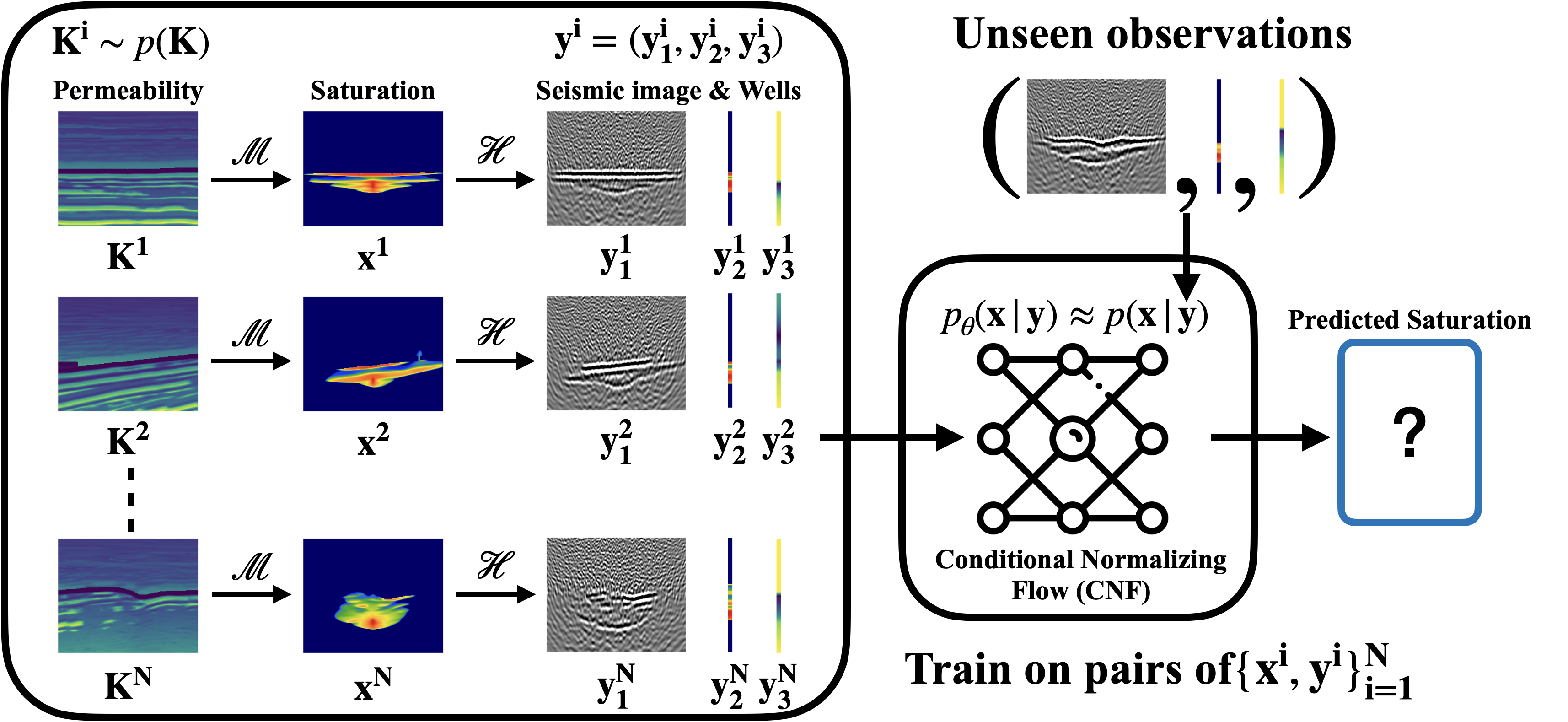
Figure 1: Creation of training and testing data for the conditional normalizing flow. Training pairs are simulated by running fluid flow simulations ($\mathcal{M}$) for random samples of the permeability ($\mathbf{K}^{(i)}\sim p(\mathbf{K}),\,i=1\cdots N$). These reservoir simulations produce samples for the CO₂ saturation, $\mathbf{x}^{(i)},\,i=1\cdots N$, and pressure. The simulated plumes are observed, via the observation operator $\mathcal{H}$, directly at the well, producing localized measurements for the saturation and pressure, and indirectly via imaged seismic reflection data collected at the surface. The conditional normalizing flow is trained on pairs of CO₂ saturation and corresponding time-lapse observations collected in the vector $\mathbf{y}^{(i)},\,i=1\cdots N$. Each $\mathbf{y}^{(i)}=(\mathbf{y}^{(i)}_{1},\mathbf{y}^{(i)}_{2},\mathbf{y}^{(i)}_{3})$ with the subscripts denoting seismic (1), saturation at well (2), and pressure at well (3), respectively. After training, the normalizing flow is tested on unseen observations.

2.1 Conditional Normalizing Flows

Normalizing flows are generative models that approximate complex target distributions by applying a series of invertible and differentiable transformations ($f_{\theta}:\mathbb{R}^{d}\rightarrow\mathbb{R}^{d}$ with inverse $f_{\theta}^{-1}$) on a base known distribution (Normal distribution)[17]. After training, normalizing flows can generate samples from the target distribution by performing the inverse operation on the base distribution. Since we want samples from the conditional distribution, we utilize conditional normalizing flows [1] where the mapping from the base density to the output space is conditioned on time-lapse observations $\mathbf{y}$ to model the posterior distribution of CO₂ saturation images, denoted as $p\left(\mathbf{x}\mid\mathbf{y}\right)$, with $\mathbf{x}$ being CO₂ saturation image and $\mathbf{y}$ being time-lapse observables. The training objective is

where $\mathbf{J}$ represents the Jacobian of the network $f_{\theta}$ with respect to its input. This training objective corresponds to minimizing the Kullback-Leibler divergence between the target density and the pull-back of the standard Gaussian distribution defined by the invertible network[21, 16]. The expectation is approximated by an average of $N$ training samples. After training, posterior samples of saturation images are generated by applying the inverse transformations to random Normal noise realizations conditioned on the observed geophysical data. These posterior samples serve as a basis for statistical analyses, including estimating the posterior variances to assess the uncertainty and to make a high-quality point estimate. We use the posterior mean calculated by the routine in Appendix A.

2.2 Dataset Generation

We select 850 2D vertical slices derived from the 3D Compass velocity model [4], to create the training dataset for our conditional normalizing flows. This model, though synthetic, is obtained from real seismic and well-log data and, thus, emulates the realistic geological characteristics prevalent in the southeastern region of the North Sea. Each 2D slice corresponds in physical dimensions to $2131\mathrm{m}\times 3200\mathrm{m}$. To simulate the dynamics of CO₂ flow, we follow [26] and convert the velocities of the Compass model [4] to models of the permeability and porosity using empirical relationships including the Kozeny-Carman equation [3]. The flow simulations are carried out with the open-source packages Jutul.jl [15] and JutulDarcyRules.jl [24] while seismic data modeling and imaging are done with JUDI [12], which is a Julia front-end to Devito [11, 14], a just-in-time compiler for industry-scale time-domain finite-difference calculations. Next, fluid flow and wave simulations are briefly discussed. Refer to [13] for more detail on the numerical simulations.

2.2.1 Fluid Flow Simulations

To obtain a realistic CO₂ injection, an injectivity of 1 MT/year is chosen with vertical injection intervals inside the high permeability regions. As CO₂ is injected supercritically, the CO₂ saturations and pressures are calculated by numerically solving the equations for two-phase flow. Details on these numerical solutions of the partial-differential equations can be found in [18]. Two distinct flow scenarios, namely regular flow (no-leakage) and irregular flow (leakage), are considered. During no-leakage, the reservoir properties are kept constant resulting in regular CO₂ plumes. However, leakage occurs when the permeability changes at the reservoir’s seal, which results in an irregular flow. While leakage can be caused by many mechanisms, we only consider the one due to pressure-induced opening of pre-existing fractures in the seal. In this case, leakage is triggered when CO₂ injection pressure reaches a predefined threshold [19], resulting in an instantaneous permeability increase within the seal causing the CO₂ plume to leak out of the reservoir. To train the CNFs, 1700 multiphase flow simulations are performed ($N=1700)$, 850 with and 850 without leakage. In practice, these fluid flow simulations can also be performed by computationally cheap surrogates based on model-parallel Fourier neural operators [6], enhancing its adaptability to large-scale four-dimensional scenarios. In the next section, we describe the formation of seismic images of these regular/irregular plumes.

2.2.2 Time-lapse Seismic Imaging

As injection of CO₂ induces changes in the Earth’s acoustic properties (velocity and density), these changes can be observed seismically. To mimic the process of collecting time-lapse seismic data followed by imaging, seismic baseline and monitor surveys are modeled. During these simulations, the baseline survey represents the initial stage before CO₂ is injected, and the monitor survey corresponds to the time of 8 years after the injection. The seismic acquisition uses 8 sources and 200 ocean bottom nodes, along with a 15 Hz Ricker wavelet and a band-limited noise term with a signal-to-noise ratio (SNR) of 8.0 dB. Reverse time migration (RTM) [2] is employed to create time-lapse seismic images of the subsurface. Then, we isolate the time-lapse changes attributed to CO₂ saturation by subtracting the baseline and monitor images.

3 Training and Results

To create training pairs, $\{\mathbf{x}^{(i)},\mathbf{y}^{(i)}\}_{i=1}^{1750}$, we resize the saturation dataset $(\mathbf{x})$ into a 256 $\times$ 256 single channel images and the time-lapse data $(\mathbf{y})$ into 256 $\times$ 256 $\times$ three channel images. The three channels are the imaged seismic observations, pressure well, and saturation well data, respectively. The architecture of the conditional normalizing flow is similar to [1]. Refer to Appendix A for further details and hyperparameter selection.

After training, the conditional normalizing flow generates samples from the posterior distribution of CO₂ saturation given unseen seismic and well observations. Figure 2 & Figure 3 show the outputs for a no-leakage case and leakage case, respectively. The posterior means of the samples appear close to the ground truth and have SSIM (see Appendix B) values of $0.97$ and $0.96$ for the no-leakage and leakage case. As expected, the uncertainty (normalized std) is higher in geologically complex areas such as the top of the plume, which corresponds to the bottom of the seal and the fracture region from where CO₂ leaks out and it also correlates well with the error. We show more test samples in Appendix B. Although there are errors in our method’s capability to find the exact extent of the plume, we do not observe any false positives or false negatives (positive and negative refer to leakage and no-leakage respectively) from the 36 test samples. In other words, all leakage scenarios are clearly inferred as leakage and all no-leakage scenarios are inferred as no-leakage.

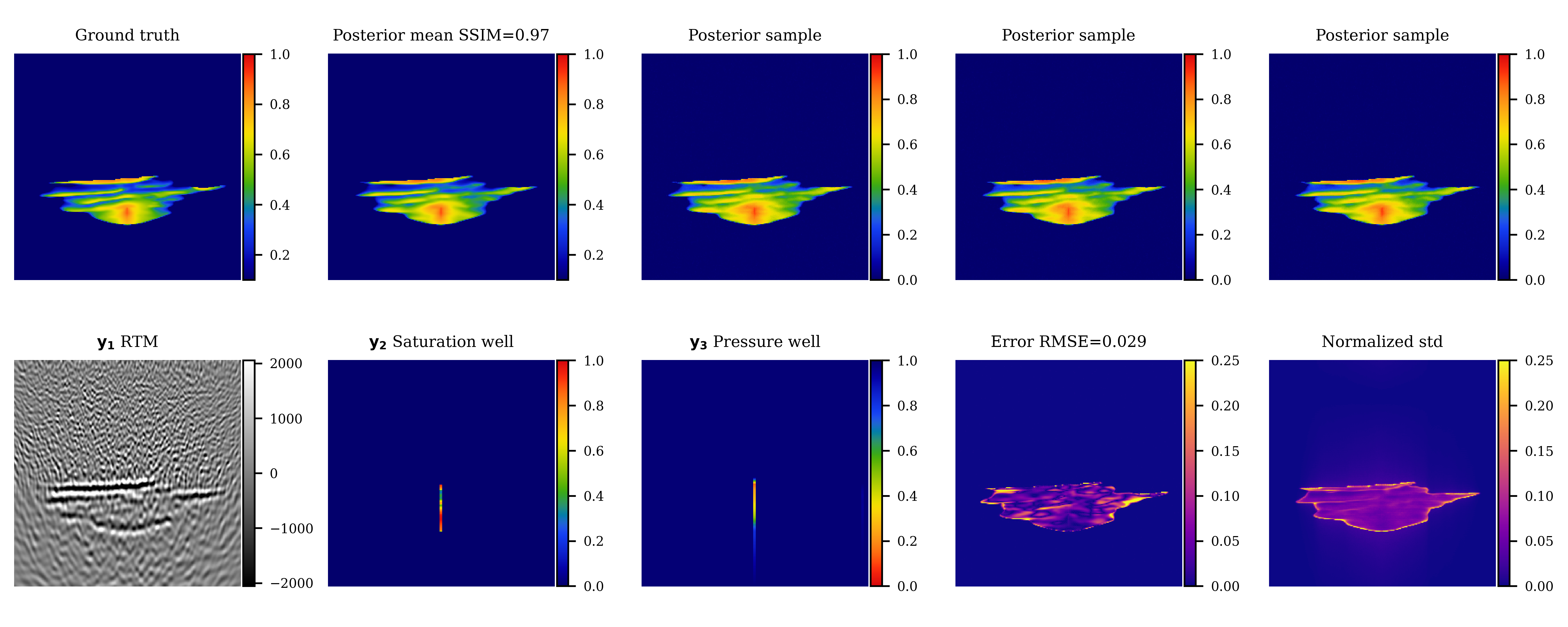
Figure 2: Outputs from the trained network for no-leakage case. Refer to Appendix B for details on performance metrics and additional examples.

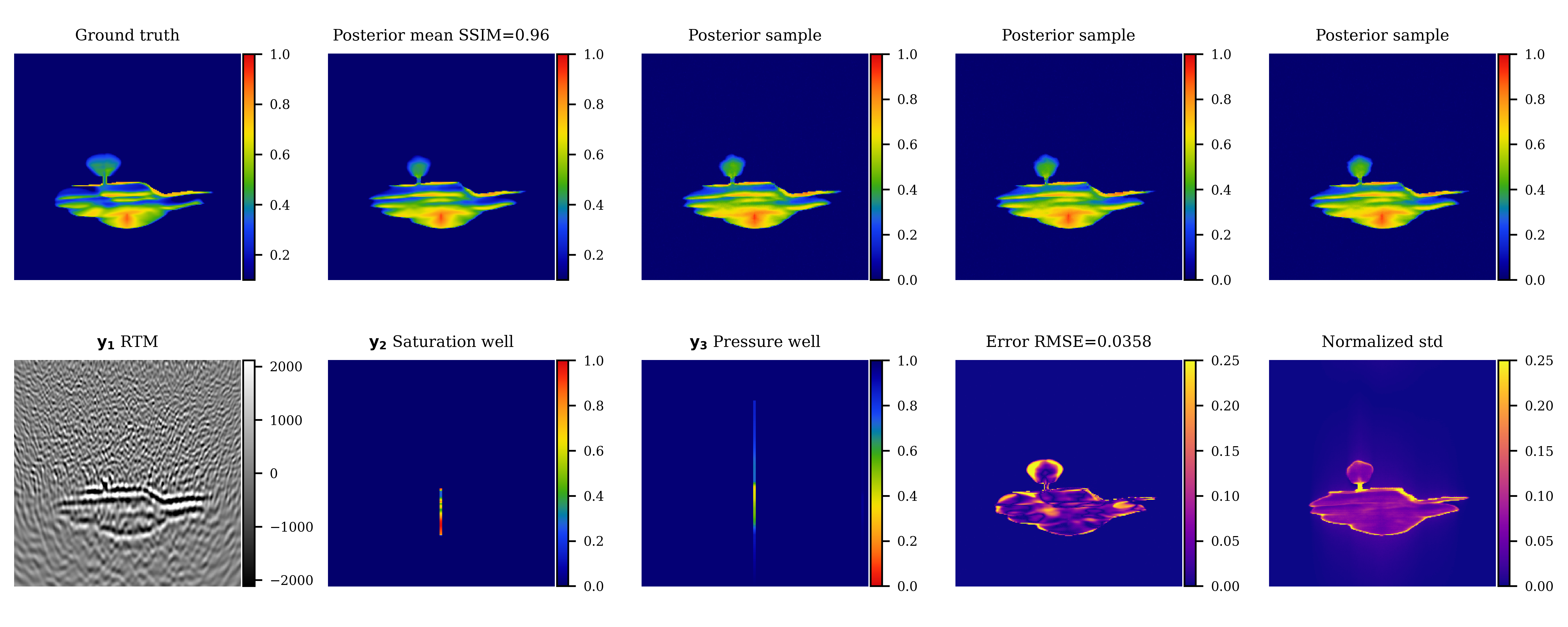
Figure 3: Same as Figure 2 but now for leakage case.

4 Conclusion and Discussion

Monitoring of GCS is complicated by highly nonlinear relationships between the reservoir properties, the CO₂ plumes, and time-lapse seismic observations. These complications are compounded by the fact that the reservoir properties are only available statistically, making it difficult to detect potential CO₂ leakages that lead to subtly differing flow patterns. By employing carefully designed numerical experiments, we are able to demonstrate that conditional normalizing flows are capable of capturing these subtle pattern changes during inference in a setting where training pairs consist of realizations for the CO₂ saturation and associated time-lapse data, consisting of seismic images and well measurements, for scenarios that include regular and irregular (leakage) flow. Aside from producing estimates for the CO₂ saturation that only differ slightly from the ground truth, these inferences also produce estimates for the uncertainty that correlate well with the errors. In future work, we will study how this type of inference can lead to an uncertainty-aware ML-based monitoring system capable of early leakage detection. This feasibility study can also serve as an initial step towards constructing a digital twin of a geological carbon storage monitoring system that receives real-time data updates, and employs simulation, machine learning, and reasoning methodologies to facilitate decision-making processes. This can be achieved by employing sequential Bayesian inference of CO₂ plumes conditioned on time-lapse geophysical observations as discussed in [7].

5 Acknowledgements

This research was carried out with the support of Georgia Research Alliance and partners of the ML4Seismic Center. This research was also supported in part by the US National Science Foundation grant OAC 2203821.

Appendix A Training Setting

We use following hyperparameters during training experiment (see Table1).

Training Hyperparameters
Batch Size	32
Optimizer	Adam [9]
Learning rate (LR)	$10^{-3}$
No. of training epochs	100
Fixed Noise Magnitude	0.005
No. of training samples	1632
No. of validation samples	68
No. of testing samples	36

Table 1: Hyperparameter for the training experiment.

After the completion of training, we use the following procedure to calculate posterior mean:

where $\hat{\theta}$ is the minimizer of Equation 1.

Appendix B Generated Examples and Useful Definitions

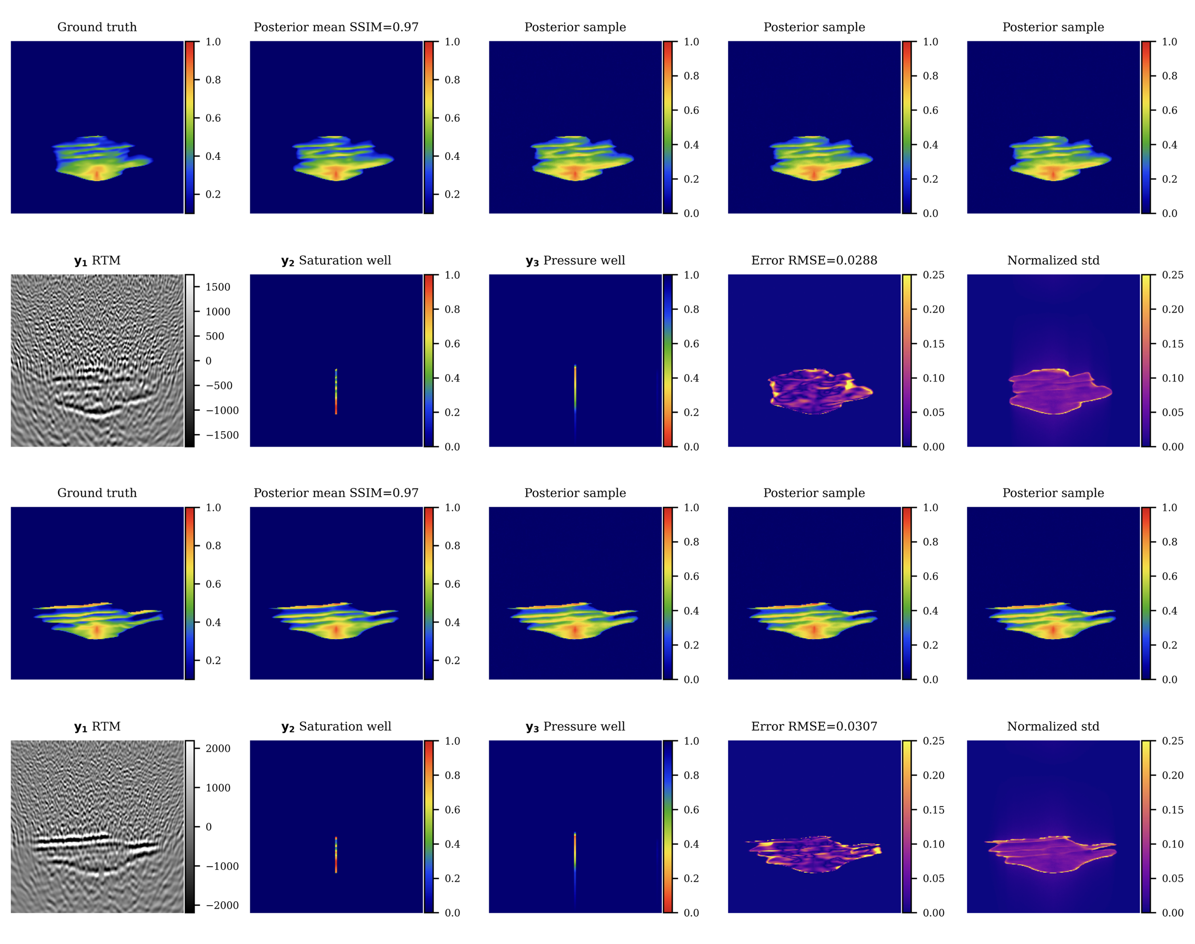
Figure 4: Two distinct examples for no-leakage scenario. In both cases, the network can generate high-fidelity saturation images with posterior mean SSIM of 0.97. Relatively larger uncertainty values are concentrated around the boundary of CO₂ plumes.

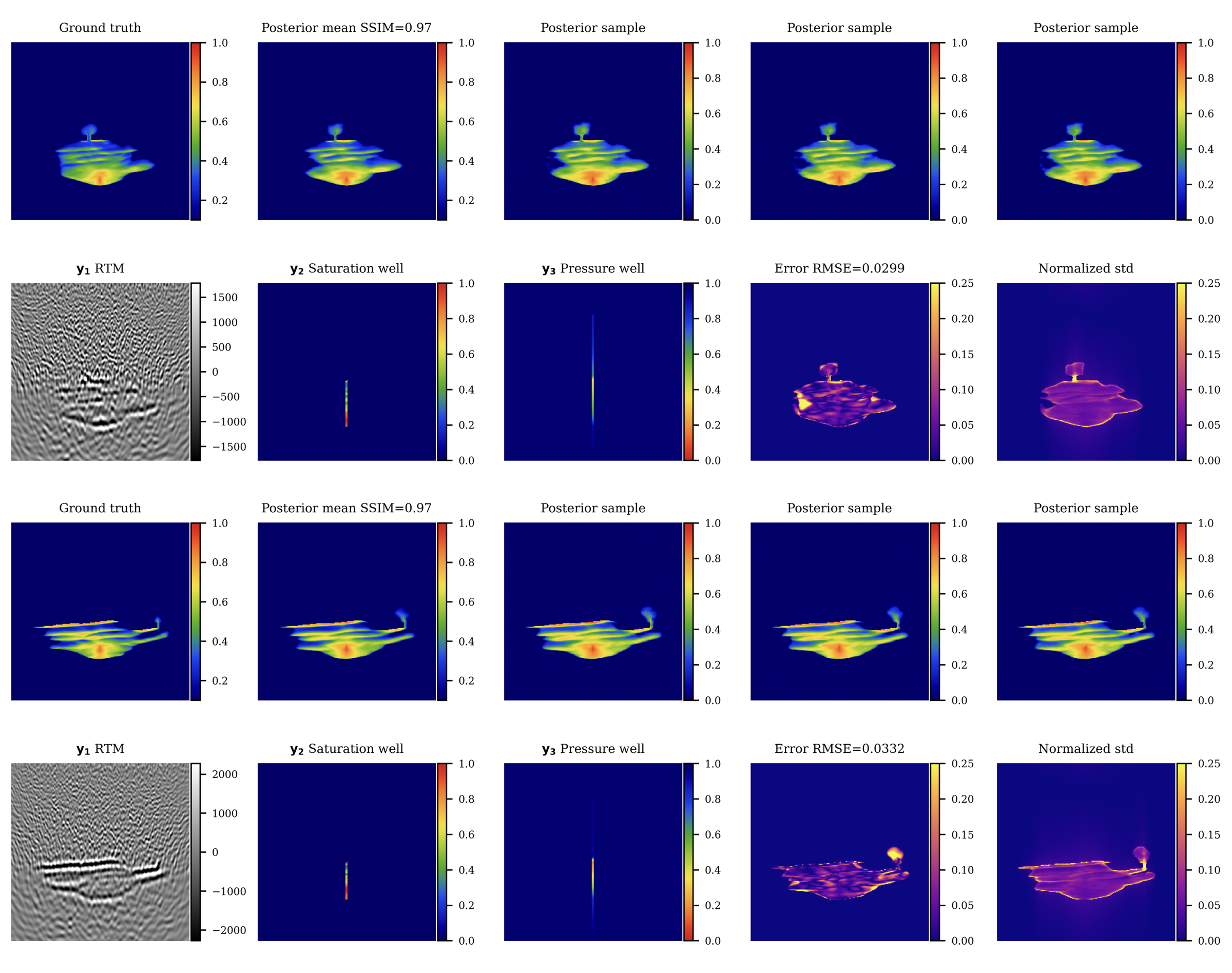
Figure 5: The corresponding leakage scenario for previous two examples. In both instances, the leakage posterior means have SSIM of 0.97. Relatively larger uncertainty values are concentrated within the area of the CO₂ leakage, particularly along the canal (fractured seal area) and the edges of the plume.

Metric definitions used in Figures 2, 3, 4 & 5 and text:

SSIM - Structural similarity index quantifies the similarity between two images and is commonly used to assess how closely a generated image resembles a ground truth or reference image. It considers image quality aspects such as luminance, contrast, and structure. For the mathematical formulation of SSIM, please refer to the study by [23].

RMSE - Root mean squared error is used to represent the measure of difference between ground truth CO₂ saturation image and the posterior mean of the samples generated by the trained network.

Normalized std - It represents normalized point-wise standard deviation or mean-normalized standard deviation. It is calculated by stabilized division of the standard deviation by the envelope of the conditional mean [21]. It is used to avoid the bias from strong amplitudes in the estimated image.

References

- Ardizzone et al. [2019] L. Ardizzone, C. Lüth, J. Kruse, C. Rother, and U. Köthe. Guided image generation with conditional invertible neural networks. CoRR, abs/1907.02392, 2019. URL http://arxiv.org/abs/1907.02392.
- Baysal et al. [1983] E. Baysal, D. D. Kosloff, and J. W. C. Sherwood. Reverse time migration. GEOPHYSICS, 48(11):1514–1524, 1983. doi: 10.1190/1.1441434. URL https://doi.org/10.1190/1.1441434.
- Costa [2006] A. Costa. Permeability-porosity relationship: A reexamination of the kozeny-carman equation based on a fractal pore-space geometry assumption. Geophysical Research Letters, 33(2), 2006. doi: https://doi.org/10.1029/2005GL025134. URL https://agupubs.onlinelibrary.wiley.com/doi/abs/10.1029/2005GL025134.
- E. Jones et al. [2012] C. E. Jones, J. A. Edgar, J. I. Selvage, and H. Crook. Building complex synthetic models to evaluate acquisition geometries and velocity inversion technologies. In 74th EAGE Conference and Exhibition Incorporating EUROPEC 2012, art. cp-293-00580, 2012. ISSN 2214-4609. doi: https://doi.org/10.3997/2214-4609.20148575. URL https://www.earthdoc.org/content/papers/10.3997/2214-4609.20148575.
- Erdinc et al. [2022] H. T. Erdinc, A. P. Gahlot, Z. Yin, M. Louboutin, and F. J. Herrmann. De-risking carbon capture and sequestration with explainable co2 leakage detection in time-lapse seismic monitoring images. arXiv preprint arXiv:2212.08596, 2022.
- Grady et al. [2023] T. J. Grady, R. Khan, M. Louboutin, Z. Yin, P. A. Witte, R. Chandra, R. J. Hewett, and F. J. Herrmann. Model-parallel fourier neural operators as learned surrogates for large-scale parametric pdes. Computers & Geosciences, page 105402, 2023.
- Herrmann [2023] F. J. Herrmann. President’s page: Digital twins in the era of generative ai. The Leading Edge, 42(11):730–732, 2023.
- IPCC [2018] IPCC. Global warming of 1.5°c. an ipcc special report on the impacts of global warming of 1.5°c above pre-industrial levels and related global greenhouse gas emission pathways, in the context of strengthening the global response to the threat of climate change, sustainable development, and efforts to eradicate poverty. In Press, 2018.
- Kingma and Ba [2014] D. P. Kingma and J. Ba. Adam: A method for stochastic optimization. CoRR, abs/1412.6980, 2014. URL https://api.semanticscholar.org/CorpusID:6628106.
- Li et al. [2018] B. Li, F. Zhou, H. Li, A. Duguid, L. Que, Y. Xue, and Y. Tan. Prediction of co2 leakage risk for wells in carbon sequestration fields with an optimal artificial neural network. International Journal of Greenhouse Gas Control, 68:276–286, 2018. ISSN 1750-5836. doi: https://doi.org/10.1016/j.ijggc.2017.11.004. URL https://www.sciencedirect.com/science/article/pii/S1750583617303237.
- Louboutin et al. [2019] M. Louboutin, M. Lange, F. Luporini, N. Kukreja, P. A. Witte, F. J. Herrmann, P. Velesko, and G. J. Gorman. Devito (v3.1.0): an embedded domain-specific language for finite differences and geophysical exploration. Geoscientific Model Development, 12(3):1165–1187, 2019. doi: 10.5194/gmd-12-1165-2019. URL https://gmd.copernicus.org/articles/12/1165/2019/.
- Louboutin et al. [2023a] M. Louboutin, P. Witte, Z. Yin, H. Modzelewski, Kerim, C. da Costa, and P. Nogueira. slimgroup/judi.jl: v3.2.3, Mar. 2023a. URL https://doi.org/10.5281/zenodo.7785440.
- Louboutin et al. [2023b] M. Louboutin, Z. Yin, R. Orozco, T. J. Grady, A. Siahkoohi, G. Rizzuti, P. A. Witte, O. Møyner, G. J. Gorman, and F. J. Herrmann. Learned multiphysics inversion with differentiable programming and machine learning. The Leading Edge, 42(7):474–486, 2023b.
- Luporini et al. [2020] F. Luporini, M. Louboutin, M. Lange, N. Kukreja, P. Witte, J. Hückelheim, C. Yount, P. H. J. Kelly, F. J. Herrmann, and G. J. Gorman. Architecture and performance of devito, a system for automated stencil computation. ACM Trans. Math. Softw., 46(1), apr 2020. ISSN 0098-3500. doi: 10.1145/3374916. URL https://doi.org/10.1145/3374916.
- Møyner et al. [2023] O. Møyner, M. Johnsrud, H. M. Nilsen, X. Raynaud, K. O. Lye, and Z. Yin. sintefmath/jutul.jl: v0.2.6, Apr. 2023. URL https://doi.org/10.5281/zenodo.7855605.
- Orozco et al. [2023] R. Orozco, M. Louboutin, A. Siahkoohi, G. Rizzuti, T. van Leeuwen, and F. J. Herrmann. Amortized normalizing flows for transcranial ultrasound with uncertainty quantification. In Medical Imaging with Deep Learning, 07 2023. URL https://slim.gatech.edu/Publications/Public/Conferences/MIDL/2023/orozco2023MIDLanf/paper.pdf. (MIDL, Nashville).
- Papamakarios et al. [2021] G. Papamakarios, E. Nalisnick, D. J. Rezende, S. Mohamed, and B. Lakshminarayanan. Normalizing flows for probabilistic modeling and inference. J. Mach. Learn. Res., 22(1), jan 2021. ISSN 1532-4435.
- Rasmussen et al. [2021] A. F. Rasmussen, T. H. Sandve, K. Bao, A. Lauser, J. Hove, B. Skaflestad, R. Klöfkorn, M. Blatt, A. B. Rustad, O. Sævareid, K.-A. Lie, and A. Thune. The open porous media flow reservoir simulator. Computers & Mathematics with Applications, 81:159–185, 2021. ISSN 0898-1221. doi: https://doi.org/10.1016/j.camwa.2020.05.014. URL https://www.sciencedirect.com/science/article/pii/S0898122120302182. Development and Application of Open-source Software for Problems with Numerical PDEs.
- Ringrose [2020] P. Ringrose. How to store CO2 underground: Insights from early-mover CCS Projects, volume 129. Springer, 2020.
- Siahkoohi et al. [2023a] A. Siahkoohi, G. Rizzuti, R. Orozco, and F. J. Herrmann. Reliable amortized variational inference with physics-based latent distribution correction. Geophysics, 88(3), 05 2023a. doi: 10.1190/geo2022-0472.1. URL https://slim.gatech.edu/Publications/Public/Journals/Geophysics/2023/siahkoohi2022ravi/paper.html. (Geophysics).
- Siahkoohi et al. [2023b] A. Siahkoohi, G. Rizzuti, R. Orozco, and F. J. Herrmann. Reliable amortized variational inference with physics-based latent distribution correction. Geophysics, 88(3):R297–R322, 2023b.
- Stepien et al. [2023] M. Stepien, C. A. Ferreira, S. Hosseinzadehsadati, T. Kadeethum, and H. M. Nick. Continuous conditional generative adversarial networks for data-driven modelling of geologic co2 storage and plume evolution. Gas Science and Engineering, 115:204982, 2023. ISSN 2949-9089. doi: https://doi.org/10.1016/j.jgsce.2023.204982. URL https://www.sciencedirect.com/science/article/pii/S2949908923001103.
- Wang et al. [2004] Z. Wang, A. Bovik, H. Sheikh, and E. Simoncelli. Image quality assessment: from error visibility to structural similarity. IEEE Transactions on Image Processing, 13(4):600–612, 2004. doi: 10.1109/TIP.2003.819861.
- Yin et al. [2023a] Z. Yin, G. Bruer, and M. Louboutin. slimgroup/jutuldarcyrules.jl: v0.2.5, Apr. 2023a. URL https://doi.org/10.5281/zenodo.7863970.
- Yin et al. [2023b] Z. Yin, H. T. Erdinc, A. P. Gahlot, M. Louboutin, and F. J. Herrmann. Derisking geologic carbon storage from high-resolution time-lapse seismic to explainable leakage detection. The Leading Edge, 42(1):69–76, 2023b.
- Yin et al. [2023c] Z. Yin, R. Orozco, M. Louboutin, and F. J. Herrmann. Solving multiphysics-based inverse problems with learned surrogates and constraints. Advanced Modeling and Simulation in Engineering Sciences, 10(1):14, 2023c. doi: 10.1186/s40323-023-00252-0.
- Zhong et al. [2019] Z. Zhong, A. Y. Sun, and H. Jeong. Predicting co2 plume migration in heterogeneous formations using conditional deep convolutional generative adversarial network. Water Resources Research, 55(7):5830–5851, 2019. doi: https://doi.org/10.1029/2018WR024592. URL https://agupubs.onlinelibrary.wiley.com/doi/abs/10.1029/2018WR024592.
- Zhou et al. [2019] Z. Zhou, Y. Lin, Z. Zhang, Y. Wu, Z. Wang, R. Dilmore, and G. Guthrie. A data-driven co2 leakage detection using seismic data and spatial-temporal densely connected convolutional neural networks. International Journal of Greenhouse Gas Control, 90:102790, 2019. ISSN 1750-5836. doi: https://doi.org/10.1016/j.ijggc.2019.102790. URL https://www.sciencedirect.com/science/article/pii/S1750583619301239.