Mixture-of-Experts for Open Set Domain Adaptation:
A Dual-Space Detection Approach

Abstract

Open Set Domain Adaptation (OSDA) aims to cope with the distribution and label shifts between the source and target domains simultaneously, performing accurate classification for known classes while identifying unknown class samples in the target domain. Most existing OSDA approaches, depending on the final image feature space of deep models, require manually-tuned thresholds, and may easily misclassify unknown samples as known classes. Mixture-of-Expert (MoE) could be a remedy. Within an MoE, different experts address different input features, producing unique expert routing patterns for different classes in a routing feature space. As a result, unknown class samples may also display different expert routing patterns to known classes. This paper proposes Dual-Space Detection, which exploits the inconsistencies between the image feature space and the routing feature space to detect unknown class samples without any threshold. Graph Router is further introduced to better make use of the spatial information among image patches. Experiments on three different datasets validated the effectiveness and superiority of our approach. The code will come soon.

1 Introduction

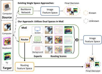
Figure 1: Comparison between existing OSDA approaches (top) and our proposed DSD (bottom). The transparency level of images corresponds to the degree of activation. DSD utilizes both the image feature space and the routing feature space in MoE to identify unknown samples, leading to improved performance.

Deep learning has made remarkable progresses in image classification [14, 5]. Nonetheless, most such models operate under the assumption that data are independently and identically distributed (i.i.d). In reality, factors such as variations in image styles and lighting conditions cause distribution shifts between source and target domain data [45], frequently degrading the generalization.

Unsupervised Domain Adaptation (UDA) [9, 25] is an approach to bridge this gap, enabling a model trained on source domain data to adapt to target domain data without using target domain labels. Traditional UDA approaches, however, often assume that the source and target domains share identical classes. In many applications, the target domain contains unknown classes, i.e., classes unseen in the source domain. Open Set Domain Adaptation (OSDA) [11, 35, 24, 1, 27, 17, 22] has been introduced to address this challenge. The goal is to handle the distribution and label shifts simultaneously, performing accurate classification for known classes while identifying unknown class samples in the target domain.

As depicted in Figure 1 (top), existing OSDA approaches predominantly use the image feature space derived from the backbone network, employing metrics like distances, classifier output probabilities, or entropy, to determine if a target domain sample belongs to an unknown class or not. However, the unknown class samples might closely resemble known class samples, and the models trained on known classes may over-confidently misclassify an unknown class sample as known [15, 4, 23]. Moreover, many existing approaches [22, 30] rely on carefully tuned thresholds, both as references and as training hyper-parameters, which may compromise the generalization and reliability of OSDA.

Mixture-of-Experts (MoE), consisting of multiple experts and a router, known for its ability to sparsify dense networks [31, 6], is an area of recent interest. Studies [28, 20] have shown that experts within the MoE demonstrate specific biases, handling distinct features within samples. The selection of these experts is governed by the router, which constructs a separate routing feature space determining the expert routing score for each sample.

This paper proposes a Dual-Space Detection (DSD) OSDA approach, which extensively makes use of the routing feature space within the MoE, as shown in Figure 1 (bottom). We assume that known classes in the target domain should be similar to known classes in the source domain in both the image feature space and the routing feature space; however, unknown classes, even if similar to known classes in the image feature space, may exhibit differences in the routing feature space. DSD identifies unknown class samples using information from both spaces, without any thresholds. Concretely, target domain samples are assigned with pseudo-labels based on distance to source domain class prototypes in both spaces, and samples with inconsistent pseudo-labels are clustered to obtain unknown class prototypes. Finally, all samples get closer to their nearest class prototypes via contrastive learning.

The router is a critical component of the MoE. Patch-wise routing [31, 6, 20] is usually used, which extracts routing features at the patch level instead of the sample-level (image-level), hindering the capture of global critical information. For each image sample, different patches can be considered as nodes in a graph [13], and the adjacency relationships between different patches form the edges of the graph. Based on this, we propose Graph Router which converts each image sample into a graph and uses a graph neural network [18, 42] to obtain a sample-level routing feature space.

Our main contributions include:

• Dual-Space Strategy: We propose a novel threshold-free OSDA approach, DSD, to identify unknown class samples in the target domain, by exploiting the inconsistencies between the image feature space and the routing feature space in MoE.

• Graph Router for MoE: We introduce Graph Router, which uses a graph neural network as the MoE router to make better use of the spatial information in images.

• State-of-the-Art Performance: Our approach outperformed multiple baselines, including state-of-the-art universal domain adaptation and OSDA approaches, on three classical OSDA datasets.

2 Related Work

This section reviews relevant literature in UDA, OSDA, and MoE.

Unsupervised Domain Adaptation: Generally, UDA techniques fall into three categories: discrepancy-based approaches, self-supervised approaches, and adversarial approaches. Discrepancy-based approaches [25, 39, 19] minimize certain divergence metrics, which measure the difference between the source and target distributions. Self-supervised approaches [12, 7, 44] typically incorporate an auxiliary self-supervised learning task to aid the model in capturing consistent features across domains and hence to facilitate adaptation. Adversarial approaches [9, 26, 36] leverage domain discriminators to promote domain-invariant feature learning. These approaches generally have difficulty in addressing label shifts between domains.

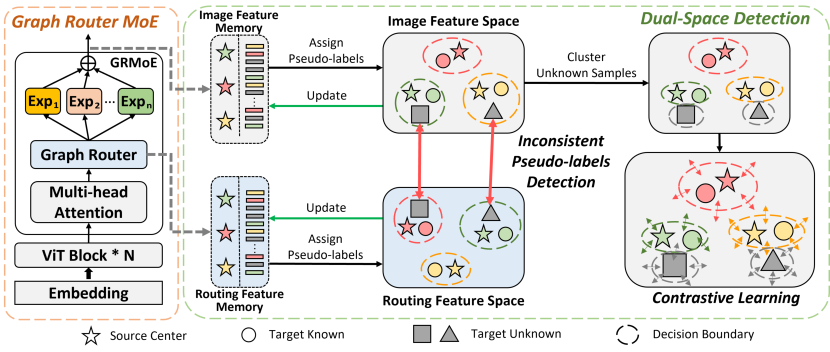
Figure 2: Graph Router MoE (left) and DSD (right). We store the model final output image features in the image feature memory, and the routing features (note they are different from the routing scores) in the routing feature memory. We then assign pseudo-labels to target domain samples in both spaces, and those with inconsistent pseudo-labels are clustered to obtain unknown class centers. Finally, we conduct contrastive learning on all samples and update both memory banks.

Open Set Domain Adaptation: OSDA handles discrepancies in known class distributions across the source and target domains, and simultaneously identify target domain unknown classes. Various strategies have been proposed. OSDA by Backpropagation (OSBP) [35] trains a classifier for target instance classification and a feature extractor to either align known class samples or reject unknown ones. Rotation-based Open Set (ROS) [1] employs rotation-based self-supervised learning to compute a normality score for known/unknown target data differentiation. Progressive Graph Learning (PGL) [27] integrates domain adversarial learning and progressive graph-based learning to refine the class-specific manifold. Unknown-Aware Domain Adversarial Learning (UADAL) [17] uses a three-class domain adversarial training approach to estimate the likelihood of target samples belonging to known classes. Adjustment and Alignment (ANNA) [22] considers the biased learning phenomenon in the source domain to achieve unbiased OSDA. Some Universal Domain Adaptation (UniDA) approaches, e.g., Domain Consensus Clustering (DCC) [21], leverage domain consensus knowledge to identify unknown samples, whereas Global and Local Clustering (GLC) [30] adopts an one-vs-all clustering strategy. All these approaches use a single feature space, and often some thresholds as hyper-parameters.

Mixture-of-Experts: An MoE model [16] includes multiple experts and a routing network. It aggregates the expert outputs via a weighted average, where the weights are determined by the routing network [6]. MoE models are sparse, resulting in reduced computational cost and increased model capacity [38]. The idea has also been extended to vision transformer (ViT) to induce block sparsity [31]. Studies [28, 20] have demonstrated MoE’s promising performance in processing visual attributes. This paper improves the routing network of MoE in ViT and extends it to OSDA, using both the image feature space and the routing feature space to more effectively identify unknown class samples.

3 Methodology

This section introduces first the formal definition of OSDA, and then our proposed DSD.

3.1 Open Set Domain Adaptation

OSDA deals with a labeled source domain and an unlabeled target domain. Assume there are $N_{s}$ labeled source domain samples $\mathcal{D}_{s}=\{(\bm{x}_{i}^{s},y_{i}^{s})\}_{i=1}^{N_{s}}$, where $\bm{x}_{i}^{s}$ is an input sample and $y_{i}^{s}$ its corresponding known class label, and $N_{t}$ unlabeled target domain samples $\mathcal{D}_{t}=\{\bm{x}_{j}^{t}\}_{j=1}^{N_{t}}$. Let $C_{s}$ be the label set in the source domain, and $C_{s}\cup y_{unk}$ the label set in the target domain, where $y_{unk}$ contains all unknown classes. The goal of OSDA is to accurately classify target domain samples from the known classes into the corresponding correct classes, and those from unknown classes into $y_{unk}$.

For a given MoE model $G$ and an input $\bm{x}$, we use $\bm{f}$ to denote the image features from the last layer of $G$, and $\bm{r}$ the routing features (note they are different from the routing scores, as will be introduced in Section 3.3).

3.2 Overview

Figure 2 illustrates our proposed DSD.

The left part of Figure 2 shows a modified ViT model [5], where a Graph Router MoE (GRMoE) layer is proposed to replace some conventional layers in the traditional ViT. More details will be presented in Section 3.3.

The right side of Figure 2 shows the flowchart of DSD. First, we feed the source and target domain samples into the source domain pre-trained model to obtain representations that will be stored in the image feature memory and the routing feature memory for source class prototypes (Section 3.4) and target domain samples (Section 3.5), respectively. Next, we assign pseudo-labels to all target samples, based on their similarities to the source class prototypes in both the image feature space and the routing feature space. Next, we cluster target samples with inconsistent pseudo-labels between these two spaces to obtain class prototypes for potential unknown classes (Section 3.6). Finally, the model is updated by minimizing a contrastive loss between all samples and all class prototypes, and the memory banks are updated accordingly (Section 3.7).

3.3 Graph Router MoE

GRMoE is shown in the left part of Figure 2. One ViT encoder block consists of a Multi-Head Self-Attention (MHSA) and a Feedforward Network (FFN) with shortcut connections [5]. Sparsifying the FFNs in ViT improves domain generalization, as it maps features into a unified space so that similar features from different domains are processed by the same experts [20]. The router maps samples into a routing feature space, which provides important information for identifying the unknown samples. We use a graph neural network [18, 42, 8] as the router to enhance the model’s ability to utilizing spatial information.

In a GRMoE layer, the FFN is replaced by an MoE, and each expert $\text{Exp}(\cdot)$ is implemented by an FFN [31, 20]. The output of GRMoE is:

$$\text{GRMoE}(\bm{x})=\sum_{i=1}^{N}\text{TOP}_{K}\{\text{Softmax}(\text{GR}(\bm{x}))\}\cdot\text{EXP}_{i}(\bm{x}),$$ (1)

where $N$ is the total number of experts, and $\bm{x}$ the output of the MHSA, including a series of image patch embeddings and a class token. $\text{TOP}_{K}(\cdot)$ is a one-hot encoding that sets all other elements in the output vector as zero except the largest $K$ elements. $\text{GR}(\cdot)$ is our proposed Graph Router:

$$\text{GR}(\bm{x})=\text{FC}(\text{Norm}(\text{GAT}(\mathcal{G}))),$$ (2)

where $\bm{x}$ is mapped into a graph $\mathcal{G}=(\mathcal{V},\mathcal{E})$. The node set $\mathcal{V}$ is the collection of the embeddings and the class token [13]. The edge set $\mathcal{E}$ is formed by connecting adjacent patches of the original image and linking every patch to the class token, as illustrated in Figure 3 (left). The graph is then input into the Graph Attention Layer [42] $\text{GAT}(\cdot)$, which is normalized by $\text{Norm}(\cdot)$ to obtain per patch routing features. The routing features are then input into a Fully Connected layer $\text{FC}(\cdot)$ to assign routing scores to the patchs and class token, as shown in Figure 3 (right). The output of the GRMoE layer is a summary of $\text{TOP}_{K}$ experts weighted by their routing scores.

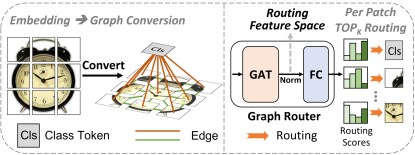
Figure 3: Overview of the Graph Router. (Left) The conversion from the embeddings to the graph. Each patch embedding serves as a node. The edges are formed by connecting adjacent patches of the original image and linking every patch to the class token. (Right) The graph is input into the Graph Router. The routing features are extracted from the GAT layer, and the routing scores are obtained from the FC layer. ‘Norm’ denotes the normalization operation.

3.4 Known Class Prototypes

For source domain samples $\mathcal{D}_{s}$ from known classes $C_{s}$, since their labels are available, the class prototypes are obtained by feeding the source samples into the model and aggregating the final image features as well as the routing features from the Router.

Specifically, the prototype of each known class is computed as the mean feature of all samples belonging to it:

$$\bm{c}_{k}^{r}=\frac{1}{|{\cal R}_{k}|}\sum_{\bm{r}_{i}\in{\cal R}_{k}}\bm{r}_{i},$$ (3)

$$\bm{c}_{k}^{f}=\frac{1}{|{\cal F}_{k}|}\sum_{\bm{f}_{i}\in{\cal F}_{k}}\bm{f}_{i},$$ (4)

where ${\cal R}_{k}$ and ${\cal F}_{k}$ denote Class $k$’s image features and routing features, respectively.

3.5 Momentum Memory

We introduce a momentum memory [10] for both the image feature space and the routing feature space to stabilize the learning. In each iteration, the encoded feature vectors in each mini-batch are used to update the momentum memory.

The prototype $\{\bm{c}^{r}_{k},\bm{c}^{f}_{k}\}$ for the $k$-th source domain class is updated as:

$$\bm{c}^{r}_{k}\leftarrow m\bm{c}^{r}_{k}+(1-m)\cdot\frac{1}{|\mathcal{B}_{k}^{r}|}\sum_{\bm{r}_{i}\in\mathcal{B}_{k}^{r}}\bm{r}_{i},$$ (5)

$$\bm{c}^{f}_{k}\leftarrow m\bm{c}^{f}_{k}+(1-m)\cdot\frac{1}{|\mathcal{B}_{k}^{f}|}\sum_{\bm{f}_{i}\in\mathcal{B}_{k}^{f}}\bm{f}_{i},$$ (6)

where $\mathcal{B}_{k}^{r}$ and $\mathcal{B}_{k}^{f}$ denote the set of source routing features and image features belonging to class $k$ in the current mini-batch, and $m\in[0,1]$ is a momentum coefficient.

The target domain samples do not have labels, so we consider each sample as a separate class. Assume the $i$-th sample in the current mini-batch is corresponding to the $i^{\prime}$-th sample in the entire target domain. Then, its features $\{\bm{r}^{t}_{i},\bm{f}^{t}_{i}\}$ are updated as:

$$\bm{r}_{i^{\prime}}^{t} \leftarrow m\bm{r}_{i^{\prime}}^{t}+(1-m)\bm{r}^{t}_{i},$$ (7)

$$\bm{f}_{i^{\prime}}^{t} \leftarrow m\bm{f}_{i^{\prime}}^{t}+(1-m)\bm{f}^{t}_{i}.$$ (8)

3.6 Unknown Class Prototypes

For an unlabeled target sample $x_{j}^{t}$, we first obtain its image features $\bm{f}^{t}_{j}$ and routing features $\bm{r}^{t}_{j}$ from the memory banks, and then compute the corresponding cosine distance $d(\cdot,\cdot)$ to each known class prototype. Two pseudo-labels $\hat{y}^{r}_{j}$ and $\hat{y}^{f}_{j}$ are next computed as:

$$\hat{y}^{r}_{j}={\arg\min}_{k}(d(\bm{r}^{t}_{j},\bm{c}_{k}^{r})),$$ (9)

$$\hat{y}^{f}_{j}={\arg\min}_{k}(d(\bm{f}^{t}_{j},\bm{c}_{k}^{f})).$$ (10)

The pseudo-label $\hat{y}_{j}$ of $x_{j}^{t}$ is obtained by:

$$\hat{y}_{j} =\left\{\begin{aligned} &\text{unknown},&\text{if $\hat{y}^{r}_{j}\neq\hat{y}^{f}_{j}$},\\ &\hat{y}^{f}_{j},&\text{if $\hat{y}^{r}_{j}=\hat{y}^{f}_{j}$}.\end{aligned}\right.$$ (11)

Table 1: Results ($\%$) on Office31. Best average HOS in bold and second best with an underline.

Approach	Amazon$\to$DSLR			Amazon$\to$Webcam			DSLR$\to$Amazon			DSLR$\to$Webcam			Webcam$\to$Amazon			Webcam$\to$DSLR			Avg
	OS*	UNK	HOS	OS*	UNK	HOS	OS*	UNK	HOS	OS*	UNK	HOS	OS*	UNK	HOS	OS*	UNK	HOS	OS*	UNK	HOS
OSBP	89.7	66.3	76.2	89.1	66.2	75.9	62.1	78.8	69.4	79.8	86.2	82.9	76.9	66.9	71.6	93.6	77.1	84.6	81.9	73.6	76.8
STA	97.3	75.4	85.0	99.0	71.7	83.2	91.5	70.7	79.7	99.7	61.0	75.7	93.4	65.4	77.0	100.0	55.4	71.3	96.8	66.6	78.7
ROS	66.5	86.3	75.1	38.4	71.7	50.0	66.3	79.8	72.4	87.9	82.2	90.0	66.5	87.0	75.4	95.1	77.7	85.5	70.1	80.8	74.7
PGL	80.1	65.1	71.8	90.1	68.3	77.7	62.0	58.0	60.0	87.1	65.3	74.6	69.6	59.2	64.0	77.3	61.8	68.7	77.7	63.0	69.5
DCC	98.7	89.8	94.0	93.9	92.8	93.3	94.5	75.2	83.8	100.0	92.8	96.3	95.2	81.2	87.6	100.0	89.2	94.3	97.1	86.8	91.6
DANCE	84.1	33.1	47.5	91.5	55.4	69.0	67.5	63.6	65.5	97.9	55.0	70.4	92.0	47.4	62.5	100.0	48.0	64.9	88.8	50.4	63.3
OVANet	92.3	89.7	91.0	91.6	91.8	91.7	51.7	99.3	68.0	96.9	100.0	98.4	86.1	96.3	90.9	100.0	85.2	92.0	86.4	93.7	88.7
GATE$\dagger$	-	-	88.4	-	-	86.5	-	-	84.2	-	-	95.0	-	-	86.1	-	-	96.7	-	-	89.5
UADAL	81.2	88.6	84.7	84.3	96.7	90.1	72.6	90.0	80.4	100.0	92.5	96.1	72.8	92.4	81.4	100.0	98.0	99.0	85.2	93.0	88.6
ANNA	94.0	73.4	82.4	94.6	71.5	81.5	73.7	82.1	77.7	99.5	97.0	98.2	73.7	82.6	77.9	100.0	89.9	94.7	89.3	82.8	85.4
GLC	85.3	90.6	87.9	86.8	93.1	89.8	92.3	98.0	95.1	94.0	96.4	95.2	91.9	97.9	94.8	98.7	96.9	97.8	91.5	95.5	93.4
DSD (Ours)	96.9	91.3	94.0	91.2	94.4	92.8	91.5	97.0	94.1	97.9	91.9	94.8	93.4	95.3	94.4	99.1	91.3	95.0	95.0	93.5	94.2

• Cited from [2].

After obtaining pseudo-labels of all target samples, those with ‘unknown’ pseudo-labels are then clustered into $n_{u}$ clusters using k-means clustering. The Silhouette criterion [32] is used to determine the optimal $n_{u}$. Given a sample $x$ in cluster $\mathcal{P}_{I}$, its Silhouette score $s(x)\in[-1,1]$ is computed as:

$$a(x) =\frac{1}{|\mathcal{P}_{I}|-1}\sum_{x_{i}\in\mathcal{P}_{I},x_{i}\neq x}d(x,x_{i}),$$ (12)

$$b(x) =\min_{J\neq I}\frac{1}{|\mathcal{P}_{J}|}\sum_{x_{i}\in\mathcal{P}_{J}}d(x,x_{i}),$$

$$s(x) =\frac{b(x)-a(x)}{\max\{a(x),b(x)\}},$$

where $a(x)$ is the average distance of $x$ to other members in the same cluster $\mathcal{P}_{I}$ (indicating cohesion), and $b(x)$ its nearest average distance to another cluster $\mathcal{P}_{J\neq I}$ (indicating separation). A high $s(x)$ means that $x$ aligns well within its own cluster and is distinct from all other clusters. We find the $n_{u}$ with the highest Silhouette score from $\{0.25C_{s},0.5C_{s},1.0C_{s},2C_{s},3C_{s}\}$, as in [20]

After clustering, each cluster serves as a pseudo unknown class. The $k$-th unknown class prototype is computed as the mean image feature of all samples in its cluster:

$$\bm{w}_{k}^{f}=\frac{1}{|{\cal P}_{k}|}\sum_{\bm{f}^{t}_{i}\in{\cal P}_{k}}\bm{f}^{t}_{i},\quad k=1,...,n_{u}$$ (13)

where ${\cal P}_{k}$ denotes cluster $k$’s image feature set.

3.7 Contrastive Learning

After obtaining the known and unknown class prototypes, given an image feature vector $\bm{f}=G(x)$, $x\in\mathcal{D}_{s}\cup\mathcal{D}_{t}$, the contrastive loss is defined as:

$$\mathcal{L}_{\bm{f}}=-\log\frac{\exp{(\langle\bm{f},\bm{z^{+}}\rangle)}}{\sum_{k=1}^{|C_{s}|}\exp{(\langle\bm{f},\bm{c}^{f}_{k}\rangle)}+\sum_{k=1}^{n^{u}}\exp{(\langle\bm{f},\bm{w}_{k}^{f}\rangle)}},$$ (14)

where $\bm{z^{+}}$ is the nearest class prototype to $\bm{f}$, and $\langle\cdot,\cdot\rangle$ the inner product between two image feature vectors to measure their similarity.

The final loss is:

$$\mathcal{L}=\mathcal{L}_{\bm{f}}+\gamma\mathcal{L}_{\text{blc}},$$ (15)

where $\mathcal{L}_{\text{blc}}$ is a regularization term to encourage balanced use of experts in MoE [38, 20] (Appendix 6), and $\gamma$ a hyper-parameter.

3.8 Inference

With the known class prototypes $\{\bm{c}^{f}_{1},\bm{c}^{f}_{2},...,\bm{c}^{f}_{|C_{s}|}\}$ and unknown class prototypes $\{\bm{w}_{1}^{f},\bm{w}_{2}^{f},...,\bm{w}_{n_{u}}^{f}\}$ from training, to perform inference for each input target domain sample, we simply identify the nearest class prototype and use its label. Note that if any of $\{\bm{w}_{1}^{f},\bm{w}_{2}^{f},...,\bm{w}_{n_{u}}^{f}\}$ is chosen as the nearest prototype, then a label $y_{unk}$ is assigned to the corresponding input target sample.

4 Experiments

This section evaluates the performance of DSD in OSDA.

4.1 Setup

Datasets. Three typical datasets were used:

1. Office31 [33], which contains 4,652 images from 31 classes in three different domains: Amazon, Webcam, and DSLR.

2. OfficeHome [43], which contains 15,500 images from 65 classes in four different domains: Art, Clipart, Product, and Real-World.

3. VisDA [29], which contains over 200,000 images from 12 classes in different domains.

$C_{s}/y_{unk}$ class split was $10/11$ on Office31, $25/40$ on OfficeHome, and $6/6$ on VisDA, following previous studies [17, 30].

Table 2: Results ($\%$) on OfficeHome. ‘Threshold-Free’ means no threshold is required. Best average HOS in bold and second best with an underline.

Approach	Threshold-Free			Art$\to$Clipart			Art$\to$Product			Art$\to$Real-World			Clipart$\to$Art			Clipart$\to$Product			Clipart$\to$Real-World
				OS*	UNK	HOS	OS*	UNK	HOS	OS*	UNK	HOS	OS*	UNK	HOS	OS*	UNK	HOS	OS*	UNK	HOS
OSBP	✗			46.8	77.2	58.3	55.3	72.0	62.6	75.8	55.6	64.2	52.6	61.8	56.8	59.2	47.1	52.5	67.7	63.5	65.5
STA	✓			60.0	56.2	58.0	83.1	47.1	60.1	90.6	49.2	63.8	68.9	63.0	65.8	74.5	49.4	59.4	77.7	51.4	61.9
ROS	✗			48.7	73.0	58.4	64.1	66.0	65.0	73.8	62.6	67.7	52.6	64.4	57.9	59.8	53.9	56.7	58.2	76.0	66.0
PGL	✗			63.8	51.3	56.9	80.2	58.4	67.6	88.7	63.4	73.9	71.0	59.0	64.4	74.1	56.4	64.1	81.4	59.5	68.8
DCC	✓			56.7	69.3	62.3	78.9	67.2	72.6	82.2	66.8	73.7	54.1	56.1	55.1	67.8	73.9	70.7	82.7	76.6	79.5
DANCE	✗			44.7	65.1	53.0	60.3	60.0	60.1	80.7	68.9	74.3	45.6	74.7	56.6	64.5	68.7	66.5	39.7	86.7	54.4
OVANet	✓			42.6	81.4	55.9	72.3	65.6	68.8	86.1	64.1	73.5	48.7	83.4	61.5	63.1	73.9	68.1	70.1	78.1	73.9
GATE$\dagger$	✓			-	-	63.8	-	-	70.5	-	-	75.8	-	-	66.4	-	-	67.9	-	-	71.7
UADAL	✗			42.6	71.3	53.4	68.6	74.6	71.5	85.7	73.2	78.9	52.1	82.5	63.9	59.9	74.8	66.5	65.4	83.7	73.4
ANNA	✗			58.5	72.3	64.7	67.6	70.8	69.2	72.7	75.3	74.0	48.9	82.5	61.4	61.7	69.9	65.6	68.4	76.4	72.2
GLC	✗			62.6	69.3	65.8	75.6	73.6	74.6	81.4	80.2	80.8	71.4	34.4	46.4	77.9	76.2	77.0	82.1	82.2	82.1
DSD (Ours)	✓			49.5	78.1	60.6	63.6	78.7	70.3	82.3	75.6	78.8	65.4	69.4	67.3	62.5	82.6	71.2	71.8	79.9	75.6
Approach	Product$\to$Art			Product$\to$Clipart			Product$\to$Real-World			Real-World$\to$Art			Real-World$\to$Clipart			Real-World$\to$Product			Avg
	OS*	UNK	HOS	OS*	UNK	HOS	OS*	UNK	HOS	OS*	UNK	HOS	OS*	UNK	HOS	OS*	UNK	HOS	OS*	UNK	HOS
OSBP	53.2	64.5	58.3	49.6	45.2	47.3	63.3	70.1	66.6	65.8	43.1	52.1	59.2	34.1	43.2	80.3	51.8	63.0	60.7	57.2	57.5
STA	70.2	62.3	66.0	57.3	54.8	56.0	86.2	57.7	69.2	77.9	53.4	63.4	59.5	43.4	50.2	86.3	41.1	55.7	74.4	52.4	60.8
ROS	48.5	63.9	55.1	44.3	73.5	55.3	66.3	83.3	73.8	68.1	59.9	63.7	48.5	71.9	57.9	71.3	46.2	56.1	58.7	66.2	61.1
PGL	72.0	60.6	65.8	63.2	52.3	57.2	82.5	60.3	69.7	73.7	59.2	65.7	63.0	51.0	56.4	83.6	60.1	69.9	74.8	57.6	65.0
DCC	55.1	78.6	64.8	51.7	73.1	60.6	76.6	73.9	75.2	75.5	55.9	64.2	57.4	65.0	60.9	79.2	74.0	76.5	68.2	69.2	68.0
DANCE	59.7	54.0	56.7	51.3	63.4	56.7	74.8	66.1	70.1	72.4	30.0	42.5	64.8	30.9	41.8	81.1	43.7	56.8	61.6	59.4	57.5
OVANet	50.1	84.8	63.0	37.3	83.5	51.6	77.4	74.8	76.1	72.3	69.0	70.6	46.5	70.7	56.1	82.5	56.1	66.8	62.4	73.8	65.5
GATE$\dagger$	-	-	67.3	-	-	61.5	-	-	76.0	-	-	70.4	-	-	61.8	-	-	75.1	-	-	69.0
UADAL	59.6	81.3	68.8	32.5	75.1	45.3	79.4	78.8	79.1	73.6	70.7	72.2	38.3	73.9	50.5	80.8	70.8	75.5	61.5	75.9	66.6
ANNA	52.0	80.9	63.3	51.1	79.6	62.2	67.8	79.6	73.2	58.8	83.5	69.0	56.1	75.7	64.4	73.0	85.6	78.8	61.4	77.7	68.2
GLC	61.5	84.5	71.2	48.5	91.6	63.4	75.1	78.2	76.6	75.9	35.4	48.2	36.1	90.2	51.6	83.4	81.2	82.3	69.3	73.1	68.3
DSD (Ours)	61.5	82.1	70.3	42.5	83.8	56.4	78.8	76.6	77.7	73.7	71.2	72.5	47.0	80.1	59.3	76.1	79.8	77.9	64.6	78.2	69.8

• Cited from [2].

Evaluation metric. As in earlier studies, HOS [1], which calculates the harmonic mean of the average accuracies of known classes (OS*) and the accuracy of unknown class (UNK):

$$\text{HOS}=\frac{2\text{OS*}\times\text{UNK}}{\text{OS*}+\text{UNK}},$$ (16)

was used as the evaluation metric.

Baselines. Our proposed DSD was compared with existing OSDA approaches, e.g., OSBP [35], Separate to Adapt (STA) [24], ROS [1], PGL [27], UADAL [17], ANNA [22], and multiple UniDA approaches in the OSDA setting, e.g., DCC [21], Domain Adaptative Neighborhood Clustering via Entropy Optimization (DANCE) [37], One-Versus-All Network (OVANet) [34], Geometric Anchor-guided Adversarial and Contrastive Learning Framework with Uncertainty Modeling (GATE) [2], and GLC [30].

Implementation details. For a fair comparison, we implemented all approaches using the ImageNet [3] pre-trained Data-efficient image Transformers Small (Deit-S) [40] backbone network, except GATE and ANNA. Our proposed DSD used Deit-S as the backbone network, keeping the same MoE structure configuration as previous work [20] (Appendix 7). Model optimization was done using Nesterov momentum SGD with momentum 0.9 and weight decay 1e-3. Batch size 64, learning rate 1e-4, $m=0.99$, $N=6$, $K=2$, and $\gamma=100$ were used for all datasets.

4.2 Experiment Results

Tables 1-3 show the performance of all algorithms on the three datasets, respectively. On average, our proposed DSD achieved the best performance on all datasets, without using any threshold.

Table 3: Results ($\%$) on VisDA. Best HOS in bold and second best with an underline.

Approach	Sy$\to$Re			Approach	Sy$\to$Re
	OS*	UNK	HOS		OS*	UNK	HOS
OSBP	25.2	39.1	30.7	OVANet	41.8	78.7	54.6
STA	65.6	80.9	72.4	GATE$\dagger$	-	-	70.8
ROS	36.5	87.0	51.4	UADAL	50.9	93.3	65.9
PGL	74.4	34.1	46.8	ANNA	37.9	83.5	52.1
DCC	56.3	86.1	68.1	GLC	55.9	93.0	69.8
DANCE	58.7	92.2	71.7	DSD (Ours)	73.5	77.7	75.5

• Cited from [2].

1. Office31 (Table 1). Our approach achieved a better balance between OS* and UNK. DSD demonstrated good recognition performance for both known and unknown classes, with an average HOS improvement of $0.8\%$ over GLC and $2.6\%$ over PGL.

2. OfficeHome (Table 2). Our approach improved UNK significantly, outperforming GLC by $5.1\%$. It also achieved the best average HOS, outperforming GATE, GLC and UADAL by $0.8\%$, $1.5\%$ and $3.2\%$, respectively.

3. VisDA (Table 3). Our approach demonstrated superior performance in differentiating known samples from unknown ones, yielding $3.7\%$ and $5.7\%$ HOS gains over STA and GLC. In contrast, other approaches biased towards higher UNK and lower OS*, suggesting they are prone to misclassify known class samples as unknown.

Generally, DSD achieved a more balanced UNK and OS*, indicating that it can well classify known classes in the target domain, while simultaneously identifying the unknown ones. Thanks to its threshold-free nature, DSD performed well across all three datasets, demonstrating good generalization.

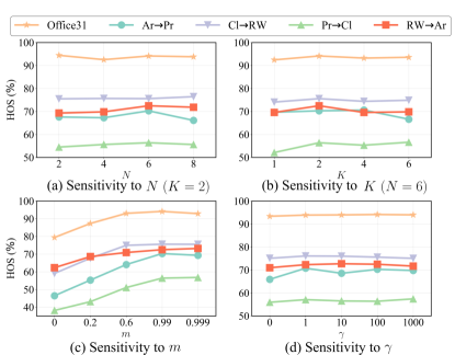
Figure 4: Parameter sensitivity analysis on Office31 and Art$\to$Product, Clipart$\to$Real-World, Product$\to$Clipart and Real-World$\to$Art on OfficeHome. (a) $N$, the total number of experts; (b) $K$, the number of experts selected during each routing step; (c) $m$ in Eq. (8); and, (d) $\gamma$.

4.3 Additional Analysis

Effect of $N$ and $K$ in MoE. The GRMoE layer includes two important hyper-parameters: $N$, the total number of experts, and $K$, the number of experts selected during each routing step. We studied the effect of each, by fixing the other. Figure 4(a) and (b) show the results. Despite the variations in $N$ and $K$, the results exhibited remarkable stability, indicating the robustness of our approach against its hyper-parameters. It further demonstrates that the remarkable performance of DSD can be traced back to the strategic exploitation of inconsistencies between two spaces, rather than an increase of model parameters.

Effect of $m$ in Momentum Update. DSD uses two separate memories to store the routing features and the image features. A momentum-based update strategy is employed during training to update these features. The influence of hyper-parameter $m$ on the performance is illustrated in Figure 4(c). A larger $m$ generally resulted in better performance, as it stabilizes the training process, which is particularly beneficial in handling the randomness in clustering unknown class samples.

Effect of $\gamma$ in the Loss Function. $\gamma$ controls the contribution of $\mathcal{L}_{\text{blc}}$ to the loss function, which promotes balanced use of the experts. Figure 4(d) shows the effect of $\gamma$. Generally, setting $\gamma>0$ is beneficial, although its specific value is not important.

Effect of the Graph Router. The routing network is very important to the performance of MoE. Many different approaches have been proposed (Appendix 8). To validate the efficacy of our proposed Graph Router, we used the widely-adopted Cosine Router [20] to replace Graph Router in the GRMoE layer. The results are shown in Table 4. Clearly, the Graph Router outperformed the Cosine Router across all three datasets. Unlike previous routers that process tokens independently, the Graph Router aggregates nearby information from adjacent tokens, enhancing the ability of experts to catch spatial critical features.

Table 4: Comparison of Cosine Router and Graph Router’s HOS (%) on the three datasets.

Router	Office31	OfficeHome	VisDA
Cosine Router	93.2	67.3	72.4
Graph Router (Ours)	94.2	69.8	75.5

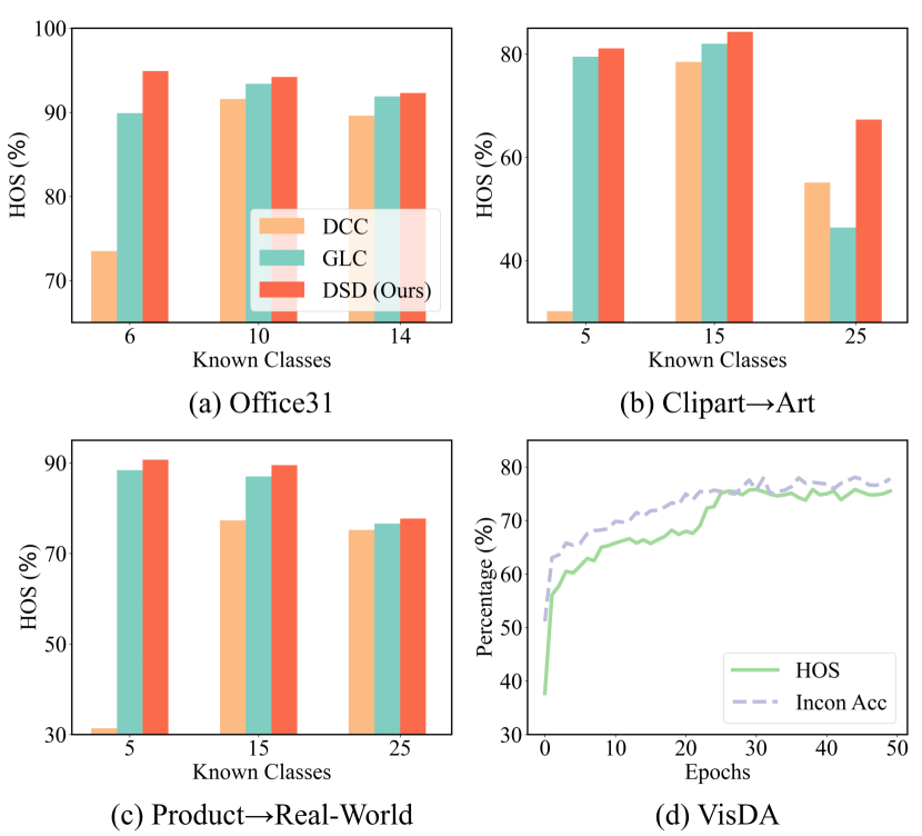
Figure 5: (a)-(c) Performance of DCC, GLC and DSD (Ours) on Office31 and Clipart$\to$Art, Product$\to$Real-World on OfficeHome with different numbers of known classes. (d) The learning curves on VisDA, where ‘Incon Acc’ denotes the percentage of samples with inconsistent pseudo-labels being from unknown classes.

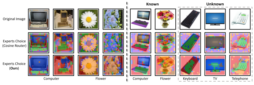
Figure 6: Visualization of the experts choice by Cosine Router and Graph Router on OfficeHome. Left: samples from the source domain (Real-World); Right: samples from the target domain (Product). Different colors represent different dominate experts. Gray dashed borders indicate unknown class samples.

4.4 Quantization Analysis

Robustness on the number of known classes. Figures 5(a)-(c) show the HOS of different approaches on Office31 and Clipart$\to$Art and Product$\to$Real-World on OfficeHome, as the number of known classes varies. Our approach always achieved the best performance, showing its ability to distinguish known and unknown samples accurately.

Learning curves. Figure 5(d) shows the learning curves of HOS and the accuracy of labeling the samples with inconsistent pseudo-labels as unknown class samples on VisDA. The recognition accuracy of unknown class samples gradually improved during the training process, leading to an increased HOS. This further demonstrates the effectiveness of DSD using the inconsistencies between two spaces to identify unknown class samples.

4.5 Visualization

Expert choice visualization. Figure 6 visualizes the routing patterns of different class samples in the MoE layer. Samples with similar features in the source and target domains are routed through similar expert pathways. For instance, the blue-colored expert is responsible for distinguishing screens, and the green-colored expert for keyboards. This pattern exists not only in the known class ‘Computer’ in the source domain but also in the unknown class samples in the target domain, validating the assumption that similar classes should also be close in the routing feature space. A close comparison of the Cosine Router and our Graph Router reveals a more consistent expert routing pattern for the latter. The proposed Graph Router exploits the spatial relationships between nearby patches, unlike the per-patch routing approaches, leading to more consistent routing patterns and hence better performance.

Feature visualization. Figure 7 shows t-SNE [41] visualization of the known and unknown target domain samples and those identified by inconsistencies in the routing feature space and the image feature space. A noticeable concentration of such inconsistent samples among the unknown samples indicates the accuracy of DSD in identifying unknown samples, and hence the validity of inconsistencies as an unknown class measure. Furthermore, the clustered centroids resemble the distribution of the unknown class samples, implying their effectiveness in capturing the potential distribution of these samples.

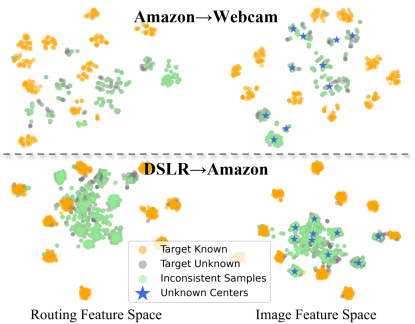
Figure 7: T-SNE visualization of the routing feature space (left) and the image feature space (right) in Amazon$\rightarrow$Webcam (top) and DSLR$\rightarrow$Amazon (bottom) on Office31.

5 Conclusion

This work has proposed a novel threshold-free DSD approach for OSDA, by considering the inconsistencies between the image feature space and the routing feature space in an MoE, enhanced by a Graph Router. DSD demonstrated promising performance in accurately identifying unknown class samples while maintaining reliable performance on known class samples, without using any thresholds. Comparisons with existing approaches demonstrated the robustness and versatility of our proposed approach, specifically shedding light on the significance of the Graph Router in leveraging spatial information among image patches.

Our future research will explore the role of the routing feature space in other applications of MoE.

Supplementary Material

6 Balanced Loss for MoE

A balanced loss $\mathcal{L}_{\text{blc}}$ is used to mitigate the potential imbalance among the experts in MoE [38, 28, 20]:

$$\mathcal{L}_{\text{blc}}=\frac{1}{2}(\mathcal{L}_{\text{imp}}+\mathcal{L}_{\text{load}}).$$ (17)

The first term, $\mathcal{L}_{\text{imp}}$, encourages a uniform distribution of routing weights among all experts. The importance of the $i$-th expert is calculated as the sum of $r_{i}(x)$ (the $i$-th component of the routing network output) for a batch $X$:

$$\text{imp}_{i}(X)=\sum\limits_{x\in X}r_{i}(x).$$ (18)

$\mathcal{L}_{\text{imp}}$ is then computed by the squared coefficient of variation of $\text{imp}(X)$:

$$\mathcal{L}_{\text{imp}}=\left(\frac{\text{Std}(\text{imp}(X))}{\text{Mean}(\text{imp}(X))}\right)^{2}.$$ (19)

The second term, $\mathcal{L}_{\text{load}}$, encourages balanced assignment across experts. The probability that the $i$-th expert is among the $\text{TOP}_{K}$ with random noise re-sampling is:

$$p_{e}(x)=1-\Phi\left(\frac{\eta_{k}-\text{EXP}_{e}({x})}{\sigma}\right),$$ (20)

where $\eta_{k}$ is the smallest entry among $\text{TOP}_{K}$, $\sigma$ the sum of noise-disrupted output of experts, and $\Phi$ the cumulative distribution function of a Gaussian distribution. The load of the $i$-th expert for a batch $X$, $\text{load}_{i}(X)$, is defined as the sum of these probabilities for all samples in that batch. Then, $\mathcal{L}_{\text{load}}$ is computed by:

$$\mathcal{L}_{\text{load}}=\left(\frac{\text{Std}(\text{load}(X))}{\text{Mean}(\text{load}(X))}\right)^{2}.$$ (21)

7 MoE Layer

We used the recommended structure in [20]: the $9$-th and $11$-th layers of the original Deit-S were replaced by GRMoE layers, and the routing feature space was obtained from the $11$-th layer’s router output. Table 5 shows results of different MoE settings, including Last Layer (only replacing the $12$-th layer of Deit-S by GRMoE) and $9$-th Routing (the output of the $9$-th GRMoE layer as the routing feature space).

As Table 5 demonstrates, our setting yielded the best performance. Specifically, utilizing the output of the $9$-th layer as the routing space led to a significant decrease in performance, indicating that features generated in earlier layers are too general to identify unknown class samples.

The poorer performance observed in the Last Layer setting may be attributed to the fact that it is too close to the model’s final image features, leading to reduced discriminability for unknown class samples.

Table 5: HOS (%) on Office31, OfficeHome, and VisDA with different MoE settings.

Setting	Office31	OfficeHome	VisDA
Last Layer	92.7	68.6	69.3
$9$-th Routing	84.3	61.8	62.6
Recommended Setting	94.2	69.8	75.5

8 Existing Routers

Existing mainstream routing network structures including Linear Router (LR),

$$\text{LR}(\bm{x})=\text{Norm}(\text{W}\bm{x}),$$ (22)

where $\bm{x}$ is the input, and W the weight matrix. The LR is too simple to deal with complex visual features [20].

The Cosine Router (CR) is

$$\text{CR}(\bm{x})=\frac{\text{E}^{T}\text{W}\bm{x}}{\tau\|\text{W}\bm{x}\|\|\text{E}\|},$$ (23)

for a given input $\bm{x}$, the embedding $\text{W}\bm{x}$ is first projected onto a hypersphere, and then multiplied by a learned embedding matrix E modulated by $\tau$.

9 Effect of the Backbone Network

To assess the impact of different backbone networks, we conducted experiments using UADAL and GLC with three different backbones: ResNet50, Deit-S, and our proposed GRMoE-sparsed Deit-S. The experimental results are presented in Table 6.

It can be observed that different backbone networks led to different performance. However, Transformer did not always outperformed ResNet. Additionally, the performance of Sparsed Deit-S was not significantly different from that of the regular Deit-S, indicating that the performance improvement of our approach was not solely due to the change in the backbone, but rather from the use of dual spaces for determining unknown class samples.

Table 6: HOS (%) of UADAL, GLC on Office31, OfficeHome, and VisDA with different backbone networks.

Approach (Backbone)	Office31	OfficeHome	VisDA
UADAL (ResNet50)	87.6	68.3	62.9
UADAL (Deit-S)	88.6	66.6	65.9
UADAL (GRMoE)	89.4	66.3	65.1
GLC (ResNet50)	88.8	65.0	58.9
GLC (Deit-S)	93.4	68.3	69.8
GLC (GRMoE)	92.8	67.4	64.4

10 More Visualization Results

Figures 8-10 give more visualization results about the expert choice on VisDA.

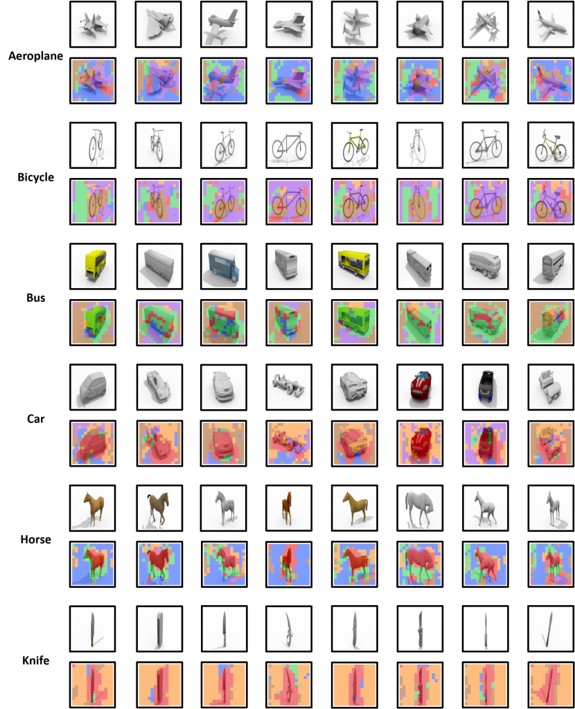
Figure 8: Visualization of expert choice on the source domain of VisDA. Different colors represent different dominate experts.

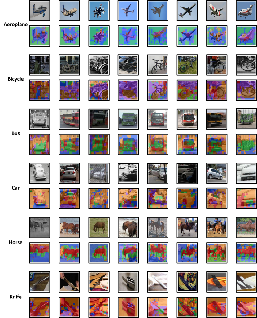
Figure 9: Visualization of expert choice on the target domain known class samples of VisDA. Different colors represent different dominate experts.

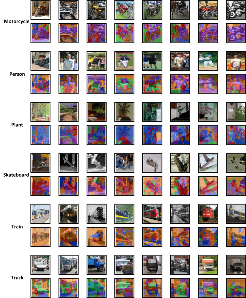
Figure 10: Visualization of expert choice on the target domain unknown class samples of VisDA. Different colors represent different dominate experts.

References

- Bucci et al. [2020] Silvia Bucci, Mohammad Reza Loghmani, and Tatiana Tommasi. On the effectiveness of image rotation for open set domain adaptation. In ECCV, pages 422–438. Springer, 2020.
- Chen et al. [2022] Liang Chen, Yihang Lou, Jianzhong He, Tao Bai, and Minghua Deng. Geometric anchor correspondence mining with uncertainty modeling for universal domain adaptation. In CVPR, pages 16134–16143, 2022.
- Deng et al. [2009] Jia Deng, Wei Dong, Richard Socher, Li-Jia Li, Kai Li, and Li Fei-Fei. Imagenet: A large-scale hierarchical image database. In CVPR, pages 248–255, 2009.
- Dhamija et al. [2018] Akshay Raj Dhamija, Manuel Günther, and Terrance Boult. Reducing network agnostophobia. In NeurIPS, 2018.
- Dosovitskiy et al. [2021] Alexey Dosovitskiy, Lucas Beyer, Alexander Kolesnikov, Dirk Weissenborn, Xiaohua Zhai, Thomas Unterthiner, Mostafa Dehghani, Matthias Minderer, Georg Heigold, Sylvain Gelly, Jakob Uszkoreit, and Neil Houlsby. An image is worth 16x16 words: Transformers for image recognition at scale. In ICLR, 2021.
- Fedus et al. [2022] William Fedus, Jeff Dean, and Barret Zoph. A review of sparse expert models in deep learning. arXiv preprint arXiv:2209.01667, 2022.
- Feng et al. [2019] Zeyu Feng, Chang Xu, and Dacheng Tao. Self-supervised representation learning from multi-domain data. In ICCV, pages 3245–3255, 2019.
- Fey and Lenssen [2019] Matthias Fey and Jan E. Lenssen. Fast graph representation learning with PyTorch Geometric. In ICLR 2019 Workshop on Representation Learning on Graphs and Manifolds, 2019.
- Ganin and Lempitsky [2015] Yaroslav Ganin and Victor Lempitsky. Unsupervised domain adaptation by backpropagation. In ICML, pages 1180–1189. PMLR, 2015.
- Ge et al. [2020] Yixiao Ge, Feng Zhu, Dapeng Chen, Rui Zhao, and Hongsheng Li. Self-paced contrastive learning with hybrid memory for domain adaptive object re-id. In NeurIPS, 2020.
- Ghaffari et al. [2023] Reyhane Ghaffari, Mohammad Sadegh Helfroush, Abbas Khosravi, Kamran Kazemi, Habibollah Danyali, and Leszek Rutkowski. Toward domain adaptation with open-set target data: Review of theory and computer vision applications. Information Fusion, 100:101912, 2023.
- Ghifary et al. [2016] Muhammad Ghifary, W Bastiaan Kleijn, Mengjie Zhang, David Balduzzi, and Wen Li. Deep reconstruction-classification networks for unsupervised domain adaptation. In ECCV, pages 597–613. Springer, 2016.
- Han et al. [2022] Kai Han, Yunhe Wang, Jianyuan Guo, Yehui Tang, and Enhua Wu. Vision gnn: An image is worth graph of nodes. In NeurIPS, pages 8291–8303, 2022.
- He et al. [2016] Kaiming He, Xiangyu Zhang, Shaoqing Ren, and Jian Sun. Deep residual learning for image recognition. In CVPR, pages 770–778, 2016.
- Hendrycks and Gimpel [2017] Dan Hendrycks and Kevin Gimpel. A baseline for detecting misclassified and out-of-distribution examples in neural networks. In ICLR, 2017.
- Jacobs et al. [1991] Robert A Jacobs, Michael I Jordan, Steven J Nowlan, and Geoffrey E Hinton. Adaptive mixtures of local experts. Neural computation, 3(1):79–87, 1991.
- Jang et al. [2022] JoonHo Jang, Byeonghu Na, Dong Hyeok Shin, Mingi Ji, Kyungwoo Song, and Il-Chul Moon. Unknown-aware domain adversarial learning for open-set domain adaptation. In NeurIPS, pages 16755–16767, 2022.
- Kipf and Welling [2017] Thomas N. Kipf and Max Welling. Semi-supervised classification with graph convolutional networks. In ICLR, 2017.
- Lee et al. [2019] Chen-Yu Lee, Tanmay Batra, Mohammad Haris Baig, and Daniel Ulbricht. Sliced wasserstein discrepancy for unsupervised domain adaptation. In CVPR, pages 10285–10295, 2019.
- Li et al. [2023a] Bo Li, Yifei Shen, Jingkang Yang, Yezhen Wang, Jiawei Ren, Tong Che, Jun Zhang, and Ziwei Liu. Sparse mixture-of-experts are domain generalizable learners. In ICLR, 2023a.
- Li et al. [2021] Guangrui Li, Guoliang Kang, Yi Zhu, Yunchao Wei, and Yi Yang. Domain consensus clustering for universal domain adaptation. In CVPR, pages 9757–9766, 2021.
- Li et al. [2023b] Wuyang Li, Jie Liu, Bo Han, and Yixuan Yuan. Adjustment and alignment for unbiased open set domain adaptation. In CVPR, pages 24110–24119, 2023b.
- Li et al. [2023c] Yushu Li, Xun Xu, Yongyi Su, and Kui Jia. On the robustness of open-world test-time training: Self-training with dynamic prototype expansion. In ICCV, pages 11836–11846, 2023c.
- Liu et al. [2019] Hong Liu, Zhangjie Cao, Mingsheng Long, Jianmin Wang, and Qiang Yang. Separate to adapt: Open set domain adaptation via progressive separation. In CVPR, pages 2927–2936, 2019.
- Long et al. [2015] Mingsheng Long, Yue Cao, Jianmin Wang, and Michael Jordan. Learning transferable features with deep adaptation networks. In ICML, pages 97–105. PMLR, 2015.
- Long et al. [2018] Mingsheng Long, Zhangjie Cao, Jianmin Wang, and Michael I Jordan. Conditional adversarial domain adaptation. In NeurIPS, 2018.
- Luo et al. [2020] Yadan Luo, Zijian Wang, Zi Huang, and Mahsa Baktashmotlagh. Progressive graph learning for open-set domain adaptation. In ICML, pages 6468–6478. PMLR, 2020.
- Mustafa et al. [2022] Basil Mustafa, Carlos Riquelme, Joan Puigcerver, Rodolphe Jenatton, and Neil Houlsby. Multimodal contrastive learning with limoe: the language-image mixture of experts. In NeurIPS, pages 9564–9576, 2022.
- Peng et al. [2017] Xingchao Peng, Ben Usman, Neela Kaushik, Judy Hoffman, Dequan Wang, and Kate Saenko. Visda: The visual domain adaptation challenge, 2017.
- Qu et al. [2023] Sanqing Qu, Tianpei Zou, Florian Röhrbein, Cewu Lu, Guang Chen, Dacheng Tao, and Changjun Jiang. Upcycling models under domain and category shift. In CVPR, 2023.
- Riquelme et al. [2021] Carlos Riquelme, Joan Puigcerver, Basil Mustafa, Maxim Neumann, Rodolphe Jenatton, André Susano Pinto, Daniel Keysers, and Neil Houlsby. Scaling vision with sparse mixture of experts. In NeurIPS, pages 8583–8595, 2021.
- Rousseeuw [1987] Peter J Rousseeuw. Silhouettes: a graphical aid to the interpretation and validation of cluster analysis. Journal of computational and applied mathematics, 20:53–65, 1987.
- Saenko et al. [2010] Kate Saenko, Brian Kulis, Mario Fritz, and Trevor Darrell. Adapting visual category models to new domains. In ECCV, pages 213–226. Springer, 2010.
- Saito and Saenko [2021] Kuniaki Saito and Kate Saenko. Ovanet: One-vs-all network for universal domain adaptation. In ICCV, pages 9000–9009, 2021.
- Saito et al. [2018] Kuniaki Saito, Shohei Yamamoto, Yoshitaka Ushiku, and Tatsuya Harada. Open set domain adaptation by backpropagation. In ECCV, pages 153–168, 2018.
- Saito et al. [2019] Kuniaki Saito, Yoshitaka Ushiku, Tatsuya Harada, and Kate Saenko. Strong-weak distribution alignment for adaptive object detection. In CVPR, pages 6956–6965, 2019.
- Saito et al. [2020] Kuniaki Saito, Donghyun Kim, Stan Sclaroff, and Kate Saenko. Universal domain adaptation through self supervision. In NeurIPS, pages 16282–16292, 2020.
- Shazeer et al. [2017] Noam Shazeer, Azalia Mirhoseini, Krzysztof Maziarz, Andy Davis, Quoc Le, Geoffrey Hinton, and Jeff Dean. Outrageously large neural networks: The sparsely-gated mixture-of-experts layer. arXiv preprint arXiv:1701.06538, 2017.
- Sun et al. [2017] Baochen Sun, Jiashi Feng, and Kate Saenko. Correlation alignment for unsupervised domain adaptation. Domain adaptation in computer vision applications, pages 153–171, 2017.
- Touvron et al. [2021] Hugo Touvron, Matthieu Cord, Matthijs Douze, Francisco Massa, Alexandre Sablayrolles, and Hervé Jégou. Training data-efficient image transformers & distillation through attention. In ICML, pages 10347–10357. PMLR, 2021.
- Van der Maaten and Hinton [2008] Laurens Van der Maaten and Geoffrey Hinton. Visualizing data using t-sne. Journal of machine learning research, 9(11), 2008.
- Veličković et al. [2018] Petar Veličković, Guillem Cucurull, Arantxa Casanova, Adriana Romero, Pietro Liò, and Yoshua Bengio. Graph attention networks. In ICLR, 2018.
- Venkateswara et al. [2017] Hemanth Venkateswara, Jose Eusebio, Shayok Chakraborty, and Sethuraman Panchanathan. Deep hashing network for unsupervised domain adaptation. In CVPR, pages 5018–5027, 2017.
- Yue et al. [2021] Xiangyu Yue, Zangwei Zheng, Shanghang Zhang, Yang Gao, Trevor Darrell, Kurt Keutzer, and Alberto Sangiovanni Vincentelli. Prototypical cross-domain self-supervised learning for few-shot unsupervised domain adaptation. In CVPR, pages 13834–13844, 2021.
- Zhao et al. [2020] Sicheng Zhao, Xiangyu Yue, Shanghang Zhang, Bo Li, Han Zhao, Bichen Wu, Ravi Krishna, Joseph E Gonzalez, Alberto L Sangiovanni-Vincentelli, Sanjit A Seshia, et al. A review of single-source deep unsupervised visual domain adaptation. IEEE Trans. on Neural Networks and Learning Systems, 33(2):473–493, 2020.