DistDNAS: Search Efficient Feature Interactions within 2 Hours

Abstract.

Search efficiency and serving efficiency are two major axes in building feature interactions and expediting the model development process in recommender systems. On large-scale benchmarks, searching for the optimal feature interaction design requires extensive cost due to the sequential workflow on the large volume of data. In addition, fusing interactions of various sources, orders, and mathematical operations introduces potential conflicts and additional redundancy toward recommender models, leading to sub-optimal trade-offs in performance and serving cost. In this paper, we present DistDNAS as a neat solution to brew swift and efficient feature interaction design. DistDNAS proposes a supernet to incorporate interaction modules of varying orders and types as a search space. To optimize search efficiency, DistDNAS distributes the search and aggregates the choice of optimal interaction modules on varying data dates, achieving over 25$\times$ speed-up and reducing search cost from 2 days to 2 hours. To optimize serving efficiency, DistDNAS introduces a differentiable cost-aware loss to penalize the selection of redundant interaction modules, enhancing the efficiency of discovered feature interactions in serving. We extensively evaluate the best models crafted by DistDNAS on a 1TB Criteo Terabyte dataset. Experimental evaluations demonstrate 0.001 AUC improvement and 60% FLOPs saving over current state-of-the-art CTR models.

1. Introduction

Recommender models vary in depth, width, interaction types and selection of dense/sparse features. These versatile feature interactions exhibit different levels of performance in recommender systems. The design of interaction between dense/sparse features is the key driver to optimizing the recommender models. The advancement of feature interactions incorporates improved prior knowledge into the recommender systems, enhancing the underlying user-item relationships and benefits personalization benchmarks such as Click-Through Rate (CTR) prediction. In past practices, there have been several advancements in feature interactions, such as collaborative filtering (Barkan and Koenigstein, 2016; Wang et al., 2016; He et al., 2017; Zhang et al., 2017). With the rise of Deep Learning (DL), factorization machines (Guo et al., 2017; Lian et al., 2018), DotProduct (Cheng et al., 2016; Naumov et al., 2019), deep crossing (Wang et al., 2021b), and self-attention (Song et al., 2019). The stack (e.g., DHEN (Zhang et al., 2022b)) and the combination (e.g., Mixture of Experts (Masoudnia and Ebrahimpour, 2014; Balog et al., 2006)) create versatile interaction types with varying orders, types, and dense/sparse input sources.

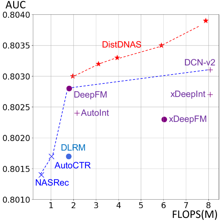
Figure 1. Model AUC versus FLOPs on Criteo Terabyte. DistDNAS unlocks 0.001 AUC compared to state-of-the-art feature interactions in recommender models.

The recent thriving of Automated Machine Learning (AutoML) democratized the design of feature interactions and exceeded human performance in various domains, such as feature selection (Liu et al., 2020) and Neural Architecture Search (Song et al., 2020; Zhang et al., 2022a; Krishna et al., 2021). Remarkably, NASRec (Zhang et al., 2022a) employs a supernet to represent the search space for recommender models and achieves state-of-the-art results on small-scale CTR benchmarks. However, optimizing feature interactions through manual design/search for large-scale CTR prediction has two challenges. First, designing/searching for the optimal feature interactions requires extensive wall-clock time, as the design/search sequentially iterates high data volume in production to obtain a good solution in feature interaction. This raises obstacles in ensuring the freshness of feature interaction on the latest data, thus potentially harming production quality, such as incurring model staleness. Thus, an efficient search methodology is pressing to explore the selection of the feature interaction and scale with the growth of the data volume. Second, fusing versatile feature interactions introduces potential conflicts and redundancy into recommender models. For example, we observe that loss divergence issues can be directly attributed to a complex interaction module (e.g., xDeepInt) with alternative feature interaction modules (e.g., CrossNet, DLRM) when training on a large dataset. This creates a sub-optimality of performance-efficiency trade-offs in service. As the relationship between model size and model performance in recommender systems has not been exploited yet, it is not certain whether fusing multiple orders and types of feature interactions into a single architecture can benefit recommender models or whether it is possible to fully harvest the improvement from different feature interactions.

In this paper, we address the above challenges and present an efficient AutoML system, Distributed Differentiable Neural Architecture Search (DistDNAS), to craft efficient feature interactions in a few hours. DistDNAS follows the setting of the supernet-based approach in NASRec (Zhang et al., 2022a) and applies Differentiable Neural Architecture Search  (Liu et al., 2018) (DNAS) to learn the structure of a feature interaction. In DistDNAS, a feature interaction is built with multiple choice blocks. Each choice block represents a linear combination of feature interaction modules (e.g., Linear, CrossNet (Wang et al., 2021b), etc.). DistDNAS presents two strong techniques to improve design efficiency and model efficiency during feature interaction search. For search efficiency, DistDNAS distributes DNAS on each training day and averages the learned weighting to derive the best combinatorial choice of interaction modules. Without ad-hoc optimizations such as embedding table sharding and communication between multiple devices, DistDNAS exhibits better scalability with a large volume of training data, achieving $\sim 25\times$ speedup on 1TB Criteo Terabyte benchmark and reducing the search cost from 2 days to 2 hours. For serving efficiency, DistDNAS calculates the cost importance of each interaction module and incorporates a differentiable cost-aware regularization loss to penalize cost-expensive interaction modules. As cost-aware regularization loss removes unnecessary interaction modules within the supernet, DistDNAS alleviates potential conflict and harvests performance improvement.

We evaluate DistDNAS on the 1TB Criteo Terabyte dataset using AUC, LogLoss and Normalized Entropy (NE) (He et al., 2014) as evaluation metrics. Without human intervention, DistDNAS removes redundant interaction modules and discovers efficient feature interactions, unlocking 0.001 higher AUC and/or 60% fewer FLOPs in the discovered models. The optimization in AUC and FLOPs brings state-of-the-art models discovered by DistDNAS, see Figure 1. We summarize our contributions as follows.

• We analyze the challenges in search efficiency and serving efficiency when designing feature interactions on large-scale CTR recommender benchmarks.

• We propose DistDNAS, an AutoML system to tackle the efficiency challenge in feature interaction design. DistDNAS distributes the search over multiple data splits and averages the learned architecture on each data split for search efficiency. In addition, DistDNAS incorporates a cost-aware regularization into the search to enhance the serving efficiency of discovered feature interactions.

• Our empirical evaluations demonstrate that DistDNAS significantly pushes the Pareto frontier of state-of-the-art CTR models.

2. Related Work

Feature Interactions in Recommender Systems. The feature interactions within recommender systems such as CTR prediction have been thoroughly investigated in various approaches, such as Logistic Regression (Richardson et al., 2007), and Gradient-Boosting Decision Trees (He et al., 2014). Recent approaches apply deep learning based interaction (Zhang et al., 2019) to enhance end-to-end modeling experience by innovating Wide & Deep Neural Networks (Cheng et al., 2016), Deep Crossing (Wang et al., 2017), Factorization Machines (Guo et al., 2017; Lian et al., 2018), DotProduct (Naumov et al., 2019) and gating mechanism (Wang et al., 2017, 2021b), ensemble of feature interactions (Zhang et al., 2022b), feature-wise multiplications (Wang et al., 2021a), and sparsifications (Deng et al., 2021). In addition, these works do not fully consider the impact of fusing different types of feature interactions, such as the potential redundancy, conflict, and performance enhancement induced by a variety of feature interactions. DistDNAS constructs a supernet to explore different orders and types of interaction modules and distributes differentiable search to advance search efficiency.

Cost-aware Neural Architecture Search. Neural Architecture Search (NAS) automates the design of Deep Neural Network (DNN) in various applications: the popularity of NAS is consistently growing in brewing Computer Vision (Zoph et al., 2018; Liu et al., 2018; Wen et al., 2020; Cai et al., 2019), Natural Language Processing (So et al., 2019; Wang et al., 2020), and Recommender Systems (Song et al., 2020; Gao et al., 2021; Krishna et al., 2021; Zhang et al., 2022a). Tremendous efforts are made to advance the performance of discovered architectures to brew a state-of-the-art model. Despite the improvement in search/evaluation algorithms, existing NAS algorithms overlook the opportunity to harvest performance improvements by addressing potential conflict and redundancy in feature interaction modules. DistDNAS regularizes the cost of the searched feature interactions and prunes unnecessary interaction modules as building blocks, yielding better FLOPs-LogLoss trade-offs on CTR benchmarks.

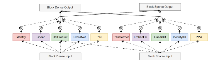
Figure 2. Feature interaction search space for each choice block in DistDNAS. Here, a dashed line denotes a searchable feature interaction in DistDNAS, and $\otimes$ denotes the mixing of different feature interaction modules.

3. Differentiable Feature Interaction Search Space

Supernet is a natural fusion that incorporates feature interaction modules. DistDNAS emphasizes search on feature interaction modules and simplifies the search space from NASRec (Zhang et al., 2022a). A supernet in DistDNAS contains multiple choice blocks, with a fixed connection between these choice blocks, and fully enabled dense-to-sparse/sparse-to-dense merger within all choice blocks. Unlike NASRec (Zhang et al., 2022a) which solely selects the optimal interaction module within each choice block, DistDNAS can select an arbitrary number of interaction modules within each choice block and use differentiable bi-level optimization (Liu et al., 2018) to determine the best selection. This allows flexibility in fusing varying feature interactions and obtaining the best combination with enhanced search efficiency. We present the details of feature interaction modules as follows.

3.1. Feature Interaction Modules

Feature interaction modules connect dense 2D inputs with sparse 3D inputs to learn useful representations on user modeling. In a recommender system, a dense input is a 2D tensor from either raw dense features or generated by dense interaction modules, such as a fully connected layer. A sparse input is a 3D tensor of sparse embeddings either generated by raw sparse/categorical features or by sparse interaction modules such as a self-attention layer. We define a dense input as $X_{d}\in\mathbb{R}^{B\times dim_{d}}$ and a sparse input $X_{s}\in\mathbb{R}^{B\times N_{s}\times dim_{s}}$. Here, B denotes the batch size, $dim_{d}$/$dim_{s}$ denotes the dimension of the dense/sparse input, and $N_{s}$ denotes the number of inputs in the sparse input.

We collect a set of simple feature interaction modules from the existing literature, as demonstrated in Figure 2. A dense interaction module produces a dense output given input features, and a sparse interaction module produces a sparse output given input features. These interaction modules can cover a set of state-of-the-art CTR models, such as DLRM (Naumov et al., 2019), DeepFM (Wang et al., 2017), xDeepInt (Yan and Li, 2023), DCN-v2 (Wang et al., 2021b), and AutoInt (Song et al., 2019).

• A Identity/Identity3D layer is a dense/sparse interaction module that carries an identity transformation on dense/sparse input. Through identity layers, one can bypass low-order interaction outputs towards deeper choice blocks and formulate a higher-order feature interaction.

• A Linear/Linear3D layer is a dense/sparse interaction module that applies on 2D/3D dense inputs, followed by a ReLU activation. Linear/Linear3D is the backbone of recommender systems since Wide & Deep Learning (Cheng et al., 2016).

• A DotProduct (Cheng et al., 2016; Naumov et al., 2019) layer is a dense interaction module that computes pairwise inner products of dense/sparse inputs. Given a dense input $X_{d}\in\mathbb{R}^{B\times dim_{d}}$ and a sparse input $X_{s}\in\mathbb{R}^{B\times N_{c}\times dim_{s}}$, a DotProduct first concatenates them as $X=Concat[X_{d},X_{s}]$, then performs pairwise inner products and collects upper triangular matrices as output: $DP(X_{d},X_{s})=Triu(XX^{T})$.

• A CrossNet (Wang et al., 2021b) layer is a dense interaction module with gate inputs from various sources. Given a dense input $X_{d}\in\mathbb{R}^{B\times dim_{d}}$, we process the dense input and the raw dense input $X_{0}$ with $CrossNet(X_{d})=sigmoid(Linear(X_{d}))*X_{0}$.

• An PIN (Yan and Li, 2023) layer is a dense interaction module with gate inputs from various sources. Given a dense input $X_{d}\in\mathbb{R}^{B\times dim_{d}}$, xDeepInt interacts the dense input with the raw dense input $X_{0}$ as follows: $PIN(X_{d})=sigmoid(Linear(X_{0}))*X_{d}$. In an xDeepInt layer, we switch the order of left/right input and perform $PIN(X_{d1},X_{d2})=X_{d1}*sigmoid(Linear(X_{d2}))$.

• A Transformer (Vaswani et al., 2017) layer is a sparse interaction module that utilizes the multihead attention mechanism to learn the weighting of different sparse inputs. The queries, keys, and values of a Transformer layer are identically the sparse input $X_{s}\in\mathbb{R}^{B\times N_{s}\times dim_{s}}$. Two Linear3D layers are then utilized to process sparse features in the embedding dimension, followed by addition and layer normalization.

• An Embedded Fully-Connected (EmbedFC) is a sparse interaction module that applies a linear operation along the middle dimension. Specifically, an EmbedFC with weights $W\in\mathbb{R}^{N_{in}\times N_{out}}$ transforms an input $X_{s}\in\mathbb{R}^{B\times N_{in}\times dim_{s}}$ to $Y_{s}\in\mathbb{R}^{B\times N_{out}\times dim_{s}}$.

• A Pooling by Multihead Attention (PMA) (Lee et al., 2019) layer is a sparse interaction module that forms attention between seed vectors and sparse features. This encourages permutation-invariant representations in aggregation. Here, PMA applies multihead attention on a given sparse input $X_{s}\in\mathbb{R}^{B\times N_{s}\times dim_{s}}$ with seed vector $V\in\mathbb{R}^{1\times N_{s}\times dim_{s}}$. PMA uses the seed vector $V$ as queries and uses sparse features as keys and values.

Within all dense/sparse interaction modules, a proper linear projection (e.g., Linear) will be applied if the dimension of inputs does not match. The feature interaction search space contains versatile dense/sparse interaction modules, providing

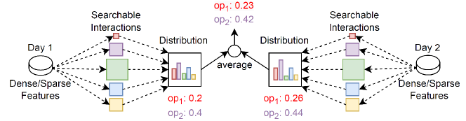
Figure 3. Overview of DistDNAS methodology. Here, dashed lines denote searchable interaction modules, and the size of interaction modules indicates the cost penalty applied to each interaction module for serving efficiency.

3.2. Differentiable Supernet

In DistDNAS, a differentiable supernet contains $N$ choice blocks with a rich collection of feature interactions. Each choice block employs a set of dense/sparse interactions $op^{(i)}=\{op_{d}^{(i)},op_{s}^{(i)}\}$ to take dense/sparse inputs $X^{(i)}_{d}$/$X^{(i)}_{s}$ and learn useful representations. Each choice block contains $|op_{d}|=5$ dense feature interactions and $|op_{s}|=5$ sparse feature interactions. Each choice block receives input from previous choice blocks and produces a dense output $Y_{d}^{(i)}$ and a sparse output $Y_{s}^{(i)}$. In block-wise feature aggregation, each choice block concatenates the dense/sparse output from the previous 2/1 choice blocks as dense/sparse block input. For dense inputs in previous blocks, the concatenation occurs in the last feature dimension. For sparse inputs in previous blocks, concatenation occurs in the middle dimension to aggregate different sparse inputs. We present the mixing of different feature interaction modules in the following context.

Continuous Relaxation of Feature Interactions. Within a single choice block in the differentiable supernet, we depict the mixing of candidate feature interaction modules in Figure 2. We parameterize the weighting of each dense/sparse/dense-sparse interaction using architecture weights. In choice block $i$, we use $\alpha^{(i)}=\{\alpha_{1}^{(i)},\alpha_{2}^{(i)},...,\alpha_{|op_{d}|}^{(i)}\}$ to represent the weighting of a dense interaction module and parameterize the selection of dense interaction modules with architecture weight $\mathrm{A}=\{\alpha^{(1)},\alpha^{(2)},...,\alpha^{(N)}\}$. Similarly, we parameterize the selection of sparse interaction modules with architecture weight $\mathrm{B}=\{\beta^{(1)},\beta^{(2)},...,\beta^{(N)}\}$. We employ the Gumbel Softmax (Jang et al., 2016) trick to allow a smoother sampling from categorical distribution on dense/sparse inputs as follows:

(1) $$Y_{d}^{(i)}=\sum_{j=1}^{|op_{d}|}\frac{\exp(\frac{\log\alpha_{j}^{(i)}+g_{j}}{\lambda})}{\sum_{k}^{|op_{d}|}\exp(\frac{\log\alpha_{k}^{(i)}+g_{k}}{\lambda})}op_{j}(X_{d}^{i},X_{d}^{i-1}),$$

(2) $$Y_{s}^{(i)}=\sum_{j=1}^{|op_{s}|}\frac{\exp{(\frac{\log\beta_{j}^{(i)}+g_{j}}{\lambda}})}{\sum_{k}^{|op_{s}|}\exp(\frac{\log{\beta_{k}}^{(i)}+g_{k}}{\lambda})}op_{j}(X_{s}^{i},X_{s}^{i-1}).$$

Here, $g_{j}$ and $g_{k}$ are sampled from the Gumbel distribution, and $\lambda$ is the temperature. As a result, a candidate architecture $\mathcal{C}$ can be represented as a tuple of dense/sparse feature interaction: $\mathcal{C}=(\mathrm{A},\mathrm{B})$. Within DistDNAS, our goal is to perform a differentiable search and obtain the optimal architecture $C^{*}$ that contains the weighting of dense/sparse interaction modules.

Discretization. Discretization converts the weighting in the optimal architecture to standalone models to serve CTR applications. Past DNAS practices (Liu et al., 2018) typically select the top k modules for each choice block, brewing a building cell containing a fixed number of modules in all parts of the network. In recommender models, we discretize each choice block by a fixed threshold $\theta$ to determine useful interaction modules. For example, in the choice block $i$, we discretize the weight $\alpha^{(i)}$ to obtain the discretized dense interaction module $\hat{\alpha}^{(i)}$ as follows:

$$\hat{\alpha}^{(i)}_{j}=\begin{cases}1,if\hat{\alpha}^{(i)}_{j}\geq\theta,\\ 0,otherwise.\\ \end{cases}$$

We typically set threshold $\theta=1/|op|$ (i.e., 0.2 for dense/sparse module search) for each choice block, or use a slightly larger value (e.g., 0.25) to remove more redundancy. There are a few advantages of adopting threshold-based discretization in recommender models. First, using a threshold $\theta$ is a clearer criterion to distinguish important/unimportant interaction modules within each choice block. Second, since a recommender model contains multiple choice blocks with different hierarchies, levels, and dense/sparse input sources, there is a need for varying numbers of dense/sparse interactions to maximize the representation capacity within each module.

4. Towards Efficiency in DNAS

Search efficiency and serving efficiency are two major considerations in deploying DNAS algorithms in large-scale CTR datasets. In this section, we first revisit DNAS and address the efficiency bottleneck via a distributed search mechanism. Then, we propose our solution to reduce the service cost of feature interaction via a cost-aware regularization approach. Figure 3 provides the core methodology of DistDNAS.

4.1. Revisiting DNAS on Recommender Systems

A Click-Through Rate (CTR) prediction task usually contains multiple days of training data. In recommender systems, we typically use a few days of data (i.e., day 1 to day $T$) as the training source and evaluate the trained model based on its CTR prediction over subsequent days. DNAS carries bilevel optimization to find the optimal candidate architecture $C^{*}=(A^{*},B^{*})$ as follows:

(3) $$(\mathrm{A}^{*},\mathrm{B}^{*})=\operatorname*{arg\,min}_{\mathrm{A},\mathrm{B}}LogLoss_{x\sim D}[x;w^{*}(\mathrm{A},\mathrm{B}),\mathrm{A},\mathrm{B}].$$

Here, $BCE$ denotes binary cross-entropy, $D=(D_{1},...,D_{T})$ indicates the training data from day 1 to day $T$, $w$ indicates the weight parameters within the DNN architecture, and $t$ indicates a certain day of data. The previous DNAS workflow must iterate over $T$ days of data, with a significant search cost. More specifically, the large search cost originates from the following considerations in search efficiency and scalability:

• Sequentially iterating over $T$ days of data requires $T$ times the search cost of DNAS on a single day of data. This creates challenges for model freshness in production environments where $T$ can be extremely large.

• Deploying the search over multiple devices may suffer from poor scalability due to communication. For example, the forward/backward process needs to shift from model parallelism to data parallelism when offloading tensors from embedding table shards to feature interaction modules.

• Within our implementation on Criteo Terabyte, the throughput on multiple NVIDIA A5000 GPUs is lower than the throughput on a single GPU during search, as demonstrated in the Queries-Per-Second (QPS) analysis in Figure 4. Thus, it is difficult to realize good scalability in the growth of computing devices in DNAS.

The above considerations point to a distributed version of DNAS, where we partition the training data, launch a DNAS procedure on each day of training data, and average the results to derive the final architecture. We hereby propose a DistDNAS search with the following bilevel optimization.

(4) $$\small(\mathrm{A}^{*},\mathrm{B}^{*})^{(t)}=\operatorname*{arg\,min}_{\mathrm{A},\mathrm{B}}LogLoss_{x\sim D_{t}}[x;w^{*}(\mathrm{A},\mathrm{B}),\mathrm{A},\mathrm{B}],$$

such that

(5) $$\small w^{*}(\mathrm{A},\mathrm{B})^{(t)}=\operatorname*{arg\,min}_{w}LogLoss_{x\sim D_{t}}[x;w(\mathrm{A},\mathrm{B}),\mathrm{A},\mathrm{B}].$$

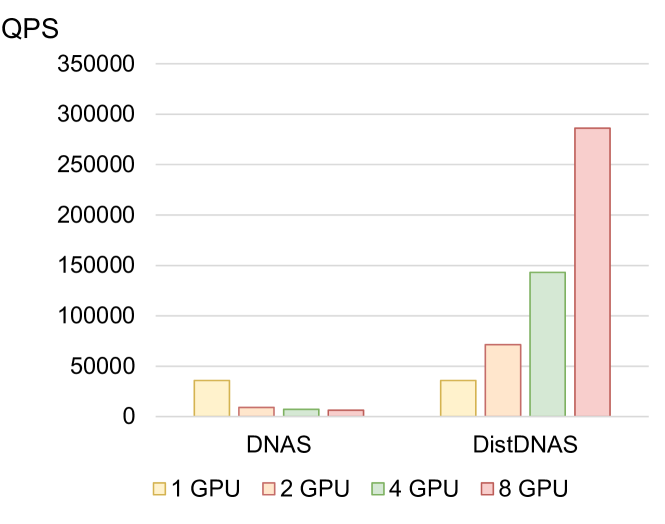
Figure 4. QPS comparison between DistDNAS and DNAS.

Here, $t\in\{1,2,..,,T\}$ indicates a certain day of training data. DistDNAS aggregates the learned weights on each day to retrieve the final architecture coefficients with a simple averaging aggregator as follows:

(6) $$\small(\mathrm{A}^{*},\mathrm{B}^{*})^{(*)}=\sum_{t=1}^{T}\frac{1}{T}(\mathrm{A}^{*},\mathrm{B}^{*})^{(t)}$$

The simple averaging scheme incorporates the statistics from each day of data to obtain the learned architecture weights. In addition, DistDNAS can be asynchronously paralleled on different computing devices, accelerating the scalability of search and reducing the total wall-clock run-time in recommender systems. Figure 4 presents a comparison of DistDNAS versus DNAS on 1-8 NVIDIA A5000 GPUs, with 4K batch size. Due to communication savings with 1-GPU training, DistDNAS benefits from significantly lower search cost compared to vanilla DNAS.

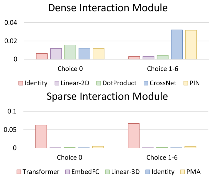
Figure 5. Normalized cost importance in a 7-block supernet.

4.2. Cost-aware Regularization

Serving cost of feature interactions, e.g. FLoating-point OPerations (FLOPs), is critical in recommender systems. A lower servicing cost indicates a shorter response time to process a user query request. As a result, optimizing the cost of recommender models is as important as optimizing the performance of recommender models in the production environment.

In DNAS, we measure the cost as a combination of training FLOPs and inference latency. The cost of a feature interaction in discovery is dependent on the weights of the learned architecture $C^{*}=(A^{*},B^{*})$. An intuition to optimize the feature interaction module is rewarding cost-efficient operators (e.g., Linear, Identity) while penalizing cost-inefficient operators (e.g., Transformer, CrossNet) during differentiable search. Motivated by this, we introduce a differentiable cost regularizer to penalize large models in discovery. The cost regularizer adds an additional regularization term $R$ to the loss function during DNAS to induce cost-effective feature interactions in discovery.

We use $j$ to represent an index of a feature interaction module in $\mathcal{C}$, for example, the index of a dense interaction module. We first sample a few pairs of architecture and cost metrics from the DistDNAS search space and create a cost mapping $cost:\mathrm{C}\to\mathrm{R}$ to model the relationship between feature interactions and FLOPs. Then, we use the permutation importance (Breiman, 2001) to obtain the importance of offline cost $s_{j}$ in the cost mapping $cost$, illustrating the offline FLOPs importance of an interaction module $i$. Finally, we formulate a cost-aware loss and incorporate it to regularize all interaction modules: $R(\mathrm{A},\mathrm{B})=\gamma\sum_{op^{j}\in(\mathrm{A},\mathrm{B})}s_{j}$. Here, $\gamma$ is an adjustable coefficient to control the strength of cost-aware regularization. With cost-aware regularization, the final architecture of DNAS with cost-aware loss searched on a single day $t$ can be formulated as follows.

(7) $$\small(\mathrm{A}^{*},\mathrm{B}^{*})^{(t)}=\operatorname*{arg\,min}_{\mathrm{A},\mathrm{B}}LogLoss_{x\sim D_{t}}[x;w^{*}(\mathrm{A},\mathrm{B}),\mathrm{A},\mathrm{B}]+R(\mathrm{A},\mathrm{B}),$$

such that

(8) $$\small w^{*}(\mathrm{A},\mathrm{B})^{(t)}=\operatorname*{arg\,min}_{w}LogLoss_{x\sim D_{t}}[x;w(\mathrm{A},\mathrm{B}),\mathrm{A},\mathrm{B}]+R(\mathrm{A},\mathrm{B}).$$

As the feature interaction search space adopts a fixed connectivity and dimension configuration during the search, the cost importance of different interaction modules is unique in the first choice block, and identical across all other choice blocks. We demonstrate the normalized cost importance of each interaction module in Figure 5. Among all interaction modules, the DotProduct contributes to a significant amount of FLOPs consumption by integrating dense and/or sparse features. Except for Transformer, sparse interaction modules contribute significantly fewer serving costs compared to their dense counterparts. Thus, despite the strong empirical performance of Transformer models, recommender models choose Transformer sparingly to build an efficient feature interaction.

Table 1. Performance of the best discovered DistDNAS model on 1TB Criteo Terabyte.

Model	FLOPS(M)	Params(M)	NE (%) $\downarrow$	Relative NE (%) $\downarrow$	AUC $\uparrow$	LogLoss $\downarrow$
DLRM (Naumov et al., 2019)	1.79	453.60	0.8462	0.0	0.8017	0.12432
DeepFM (Guo et al., 2017)	1.81	453.64	0.845	-0.14	0.8028	0.12413
xDeepFM (Lian et al., 2018)	6.03	454.14	0.846	-0.02	0.8023	0.12429
AutoInt (Song et al., 2019)	2.16	453.80	0.8455	-0.08	0.8024	0.12421
DCN-v2 (Wang et al., 2021b)	8.08	459.91	0.845	-0.14	0.8031	0.12413
xDeepInt (Yan and Li, 2023)	8.08	459.91	0.8455	-0.08	0.8027	0.12421
NASRec-tiny (Zhang et al., 2022a)	0.57	452.47	0.8463	0.01	0.8014	0.12437
AutoCTR-tiny (Song et al., 2020)	1.02	452.78	0.8460	-0.02	0.8017	0.12429
DistDNAS	1.97	453.62	0.8448	-0.17	0.8030	0.12410
	$3.11^{*}$	454.70	0.8444	-0.21	0.8032	0.12405
DistDNAS (M=2)	3.94	455.48	0.8448	-0.17	0.8033	0.12410
DistDNAS (M=3)	5.90	457.31	0.8440	-0.26	0.8035	0.12399
DistDNAS (M=4)	7.87	459.14	0.8438	-0.29	0.8039	0.12395

5. Experiments

We thoroughly examine DistDNAS on Criteo Terabyte. We first introduce the experiment settings of DistDNAS that produce efficient feature interaction in discovery. Then, we compare the performance of models crafted by DistDNAS versus a series of metrics with strong hand-crafted baselines and AutoML baselines.

5.1. Experiment Setup

We illustrate the key components of our experiment setup and elaborate on the detailed configuration.

Training Dataset. Criteo Terabyte contains 4B training data on 24 different days. Each data item contains 13 integer features and 26 categorical features. Each day of data on Criteo Terabyte contains $\sim$ 0.2B data. During the DistDNAS search, we use data from day 1 to day 22 to learn architecture the optimal architecture weights: $C^{*}=(A^{*},B^{*})$. During the evaluation, we use the data from day 1 to day 23 as a training dataset and use day 24 as a holdout testing dataset. We perform inter-day data shuffling during training, yet iterate over data from day 1 to day 23 in a sequential order.

Data Preprocessing. We do not apply any special preprocessing to dense features except for normalization. For sparse embedding tables, we cap the maximum embedding table size to 5M, and use an embedding dimension of 16 to obtain each sparse feature. Thus, each model contains $\sim$450M parameters in the embedding table.

Optimization. We train all models from scratch without inheriting knowledge from other sources, such as pre-trained models or knowledge distillation. We use different optimizers for sparse embedding parameters and dense parameters (e.g., other parameters except for sparse embedding parameters). For sparse parameters, we utilize Adagrad with a learning rate of 0.04. For dense parameters, we use Adam with a learning rate of 0.001. No weight decay is performed. During training, we use a fixed batch size of 8192, with a fixed learning rate schedule after initial warm-up. We enable Auto-Mixed Precision (AMP) to speed up training.

Architecture Search. Our supernet contains $N=7$ choice blocks during the search. We choose $\gamma$=0.004 for cost-aware regularization to balance trade-offs between performance. During the search, we linearly warm up the learning rate from 0 to maximum with 10K warm-up steps, and use a batch size of 8K to learn the architecture weights while optimizing the DNAS supernet. Each search takes $\sim$ 2 GPU hours on an NVIDIA A5000 GPU.

Discretization. During discretization, we only attempt on 0.25/0.2, and select the discovered feature interaction with a better performance/FLOPs trade-off as the product of the search. As most baseline models are larger, we naively stack $M$ copies of feature interactions in parallel to match the FLOPs of large models, such as DCN-v2 (Wang et al., 2021b) and xDeepInt (Yan and Li, 2023). In Table 1, we use $\theta$=0.20 as the discretization threshold for DistDNAS marked with $*$, and use $\theta=0.25$ to other feature interactions created by DistDNAS. We use the discovered feature interaction to connect raw dense/sparse inputs and craft a recommender model as the product of search.

Training. To ensure a fair comparison and better demonstrate the strength of the discovered models, we employ the aforementioned optimization methodologies without hyperparameter tuning. We linearly warm up the learning rate from 0 to maximum using the first 2 days of training data. To prevent overfitting, we use single-pass training and iterate the whole training dataset only once.

Baselines. We select the popular hand-crafted design choice of CTR models from the existing literature to serve as baselines, i.e., DLRM (Naumov et al., 2019), DeepFM (Guo et al., 2017), xDeepFM (Lian et al., 2018), AutoInt (Song et al., 2019), DCN-v2 (Wang et al., 2021b) and xDeepInt (Yan and Li, 2023). We also incorporate the best models from the NAS literature: AutoCTR (Song et al., 2020) and NASRec (Zhang et al., 2022a) to serve as baselines and use the best model discovered for Criteo Kaggle.

Without further specification, all hand-crafted or AutoML baselines use $dim_{s}=16$ as the embedding dimension. All hand-crafted or AutoML baselines use 512 or $dim_{d}=256$ units in the MLP layer, including 1 MLP layer in dense feature processing and 7 MLP layer in aggregating high-level dense/sparse features. All AutoML models use $N_{s}=16$ for sparse interaction modules. This ensures a fair comparison between hand-crafted and AutoML models, as the widest part in hand-crafted/AutoML models does not exceed 512. All hand-crafted feature interactions (e.g., CrossNet) are stacked 7 times to match $N=7$ blocks in the AutoML supernet, as NASRec, AutoCTR, and proposed DistDNAS employ $N=7$ blocks for feature interaction. As a result, the FLOPs cost of AutoCTR (Song et al., 2020) and NASRec (Zhang et al., 2022a) reduces significantly. We name the derived NAS baselines NASRec (tiny) and AutoCTR (tiny). We implement all of the baseline feature interactions based on open-source code and/or paper demonstration.

5.2. Evaluation on Criteo Terabyte

We use DistDNAS to represent the performance of the best models discovered by DistDNAS and compare performance against a series of cost metrics such as FLOPs and parameters. We use AUC, Normalized Entropy (NE) (He et al., 2014), and LogLoss as evaluation metrics to measure model performance. We also calculate the testing NE of each model relative to DLRM and demonstrate relative performance. Note that relative NE is equivalent to relative LogLoss on the same testing day of data. Table 1 summarizes our evaluation of DistDNAS. Here, $M$ indicates the number of parallel stackings we apply on DistDNAS to match the FLOPs of baseline models.

Upon transferring to large datasets, previous AutoML models (Song et al., 2020; Zhang et al., 2022a) searched on smaller datasets are less competitive when applied to large-scale Criteo Terabyte. This is due to sub-optimal architecture transferability from the source dataset (i.e., Criteo Kaggle) to the target dataset (i.e., Criteo Terabyte). Among all baseline models, DCN-v2 achieves state-of-the-art performance on Criteo Terabyte with the lowest LogLoss/NE and highest AUC. Despite the same parameter count and FLOPs, xDeepInt shows 0.06% NE degradation, due to the sub-optimal interaction design compared to the cross-net interaction modules.

DistDNAS shows remarkable model efficiency by establishing a new Pareto frontier on AUC/NE versus FLOPs. With a discretization threshold of 0.25, the 1.97M DistDNAS model outperforms tiny baseline models such as DLRM and DeepFM, unlocking at least 0.02% AUC/NE with on-par FLOPs complexity. With a discretization threshold of 0.2, we achieve better AUC/NE as state-of-the-art DCN-v2 models, yet with a reduction of over 60% FLOPS. By naively stacking more blocks in parallel, DistDNAS achieves the state-of-the-art AUC/NE and outperforms DCN-v2 by 0.001 AUC.

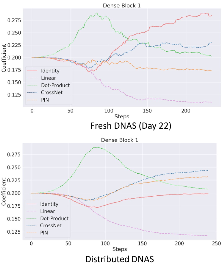
Figure 6. Comparison of learned architecture weights of dense interaction modules in choice block 1.

6. Discussion

In this section, we conduct ablation studies and analyze various confounding factors within DistDNAS, including the effect of distributed search, the effect of cost-aware regularization, and the analysis of performance on state-of-the-art models under a recurring training setting.

6.1. DistDNAS Search Strategy

DistDNAS proposes distributed search and cost-aware regularization as the main contribution. Upon applying DNAS to the recommender systems, we discuss the alternative choices to DistDNAS as follows.

SuperNet indicates a direct use of the DistDNAS supernet as a feature interaction module. No search is performed.

Distributed DNAS applies the DistDNAS search process in a distributed manner, but does not involve cost-aware regularization. Both distributed DNAS and DistDNAS take 2 hours to complete on NVIDIA A5000 GPUs.

One-shot DNAS kicks off DNAS and iteratively over the entire search data set (that is, 22 days in Criteo Terabyte) to obtain the best architecture. Despite the inefficiency of the search discussed in Section 4, a single shot DNAS on multiple days of training data cannot converge to a standalone architecture, with loss divergence during training on a large-scale dataset. Running a one-shot DNAS takes $\sim$ 50 GPU hours on an NVIDIA A5000 GPU.

Fresh DNAS only covers the most recent data in the training data set (i.e. day 22 on Criteo Terabyte) and performs a search to learn the best architecture. Intuitively, this serves as a strong baseline, as the testing data set is more correlated with the most recent data due to model freshness. We compare the learning dynamics of the architecture weights for fresh DNAS (Day-22) versus Distributed DNAS. Thanks to the averaging mechanism, Distributed DNAS benefits from more robust learning dynamics and shows smoother progress toward the learned architecture weights, see Figure 6.

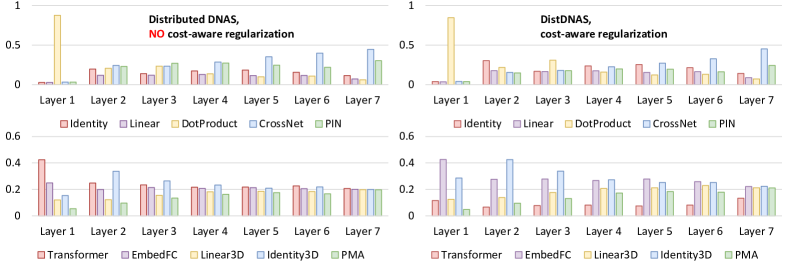
Figure 7. Comparison of learned architecture weights under distributed DNAS versus DistDNAS.

DistDNAS applies all the techniques proposed in this paper, including distributed search and cost-aware regularization. Figure 7 shows a comparison of the learned architecture weights in Distributed DNAS versus DistDNAS. DistDNAS is more likely to preserve cost-efficient interaction modules, such as EmbedFC/Identity compared to distributed DNAS without cost-aware regularization.

We perform each of the aforementioned searches and evaluate different search strategies based on the following questions:

• (Search Convergence) Whether the search converges to a stable architecture weight and produces a feature interaction in discovery?

• (Training Convergence) Does the discovered feature interaction converge on a large-scale Criteo Terabyte benchmark with 24 days of training data?

• (Testing Quality) What is the quality of the interactions of the features discovered?

Table 2. Study of different DistDNAS search strategies.

Strategy	Searching	Training	Testing
	Converge?	Converge?	FLOPs/NE
SuperNet	N/A	No	N/A
One-shot DNAS	No	No	N/A
Freshness DNAS	Yes	No	N/A
Distributed DNAS	Yes	Yes	3.56M/0.8460
DistDNAS	Yes	Yes	3.11M/0.8444

Table 2 summarizes a study of different search strategies for these questions. We have a few findings regarding the use of distributed search and the use of cost-aware regularization.

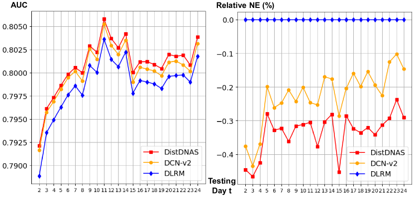
Figure 8. Comparison of AUC and Relative NE on Criteo terabyte under recurring training setting.

A standalone supernet cannot converge when trained on Criteo Terabyte dataset. This indicates that varying feature interactions may have conflicts with each other, increasing the difficulty of performing search and identify promising feature interactions.

On a large-scale dataset such as Criteo Terabyte, distributing DNAS over multiple-day splits and aggregating the learned weight architectures are critical to the convergence of search and training. This is because in recommender systems, there might be an abrupt change in different user behaviors across/intra-days; thus, a standalone architecture learned on a single day may not be suitable to capture the knowledge and fit all user-item representations. Additionally, as NAS may overfit the target dataset, a standalone feature interaction searched on day $X$ may not be able to learn day $Y$ well and is likely to collapse due to changes in user behavior.

We also compare distributed DNAS with DistDNAS to demonstrate the importance of cost-aware regularization. Experimental evaluation demonstrates that FLOPS-regularization enhances the performance of searched feature interaction, removing the redundancy contained in the supernet. This observation provides another potential direction for recommender models to compress unnecessary characteristics and derive better recommender models, such as the usage of pruning. A more recent study using an instance-guided mask (Wang et al., 2021a) supports the feasibility of applying model compression to advance performance on recommender models.

6.2. Performance Analysis under Recurring Training Scenario

Recurring training (He et al., 2014) is a common practice in recommender system applications. In recurring training, practitioners must regularly update the model on the latest data to gain fresh knowledge. Here, we simulate the scenario in recurring training to evaluate top-performing feature interactions (i.e., DistDNAS and DCN-v2) on different training/evaluation splits of Criteo Terabyte. More specifically, we use day 1 to day $t$ as training dates, and day $t+1$ as testing date to report AUC and relative NE. In Criteo Terabyte, $t$ can choose from {2, 3, 4,…, 24}.

We demonstrate the evaluation of recurring training on DistDNAS, DCN-v2 and DLRM (baseline) in Figure 8. Although performing better on the final testing date, DistDNAS consistently outperforms the previous state-of-the-art DCN-v2 on all testing splits under recurring training. This indicates that DistDNAS successfully injects the implicit patterns contained within the large-scale dataset into the searched feature interaction, learning a better prior to gain knowledge from a large amount of training data. As DistDNAS can be highly paralleled with only a single pass of the dataset, we envision that it can be beneficial for large-scale applications in search efficiency and serving efficiency.

7. Conclusion

In this article, we emphasize search efficiency and serving efficiency in the design of feature interactions through a differentiable supernet. We propose DistDNAS to explore the differentiable supernet containing various dense and sparse interaction modules. We distribute the search on different days of training data to advance search scalability, reducing end-to-end search cost from 2 days to 2 hours with a 25$\times$ speed-up in scalability. In addition, DistDNAS incorporates cost-aware regularization to remove potential conflicts and redundancies within feature interaction modules, yielding higher serving efficiency in searched architectures. Our empirical evaluation justifies the search efficiency of DistDNAS on Criteo Terabyte dataset, reducing search cost from 2 days to 2 hours. Despite search efficiency, DistDNAS discovers an efficient feature interaction to benefit serving, advancing AUC by 0.001 and surpassing existing hand-crafted/AutoML interaction designs.

References

- (1)
- Balog et al. (2006) Krisztian Balog, Leif Azzopardi, and Maarten De Rijke. 2006. Formal models for expert finding in enterprise corpora. In Proceedings of the 29th annual international ACM SIGIR conference on Research and development in information retrieval. 43–50.
- Barkan and Koenigstein (2016) Oren Barkan and Noam Koenigstein. 2016. Item2vec: neural item embedding for collaborative filtering. In 2016 IEEE 26th International Workshop on Machine Learning for Signal Processing (MLSP). IEEE, 1–6.
- Breiman (2001) Leo Breiman. 2001. Random forests. Machine learning 45 (2001), 5–32.
- Cai et al. (2019) Han Cai, Chuang Gan, Tianzhe Wang, Zhekai Zhang, and Song Han. 2019. Once-for-all: Train one network and specialize it for efficient deployment. arXiv preprint arXiv:1908.09791 (2019).
- Cheng et al. (2016) Heng-Tze Cheng, Levent Koc, Jeremiah Harmsen, Tal Shaked, Tushar Chandra, Hrishi Aradhye, Glen Anderson, Greg Corrado, Wei Chai, Mustafa Ispir, et al. 2016. Wide & deep learning for recommender systems. In Proceedings of the 1st workshop on deep learning for recommender systems. 7–10.
- Deng et al. (2021) Wei Deng, Junwei Pan, Tian Zhou, Deguang Kong, Aaron Flores, and Guang Lin. 2021. Deeplight: Deep lightweight feature interactions for accelerating ctr predictions in ad serving. In Proceedings of the 14th ACM international conference on Web search and data mining. 922–930.
- Gao et al. (2021) Chen Gao, Yinfeng Li, Quanming Yao, Depeng Jin, and Yong Li. 2021. Progressive feature interaction search for deep sparse network. Advances in Neural Information Processing Systems 34 (2021), 392–403.
- Guo et al. (2017) Huifeng Guo, Ruiming Tang, Yunming Ye, Zhenguo Li, and Xiuqiang He. 2017. DeepFM: a factorization-machine based neural network for CTR prediction. arXiv preprint arXiv:1703.04247 (2017).
- He et al. (2017) Xiangnan He, Lizi Liao, Hanwang Zhang, Liqiang Nie, Xia Hu, and Tat-Seng Chua. 2017. Neural collaborative filtering. In Proceedings of the 26th international conference on world wide web. 173–182.
- He et al. (2014) Xinran He, Junfeng Pan, Ou Jin, Tianbing Xu, Bo Liu, Tao Xu, Yanxin Shi, Antoine Atallah, Ralf Herbrich, Stuart Bowers, et al. 2014. Practical lessons from predicting clicks on ads at facebook. In Proceedings of the eighth international workshop on data mining for online advertising. 1–9.
- Jang et al. (2016) Eric Jang, Shixiang Gu, and Ben Poole. 2016. Categorical reparameterization with gumbel-softmax. arXiv preprint arXiv:1611.01144 (2016).
- Krishna et al. (2021) Ravi Krishna, Aravind Kalaiah, Bichen Wu, Maxim Naumov, Dheevatsa Mudigere, Misha Smelyanskiy, and Kurt Keutzer. 2021. Differentiable NAS Framework and Application to Ads CTR Prediction. arXiv preprint arXiv:2110.14812 (2021).
- Lee et al. (2019) Juho Lee, Yoonho Lee, Jungtaek Kim, Adam Kosiorek, Seungjin Choi, and Yee Whye Teh. 2019. Set transformer: A framework for attention-based permutation-invariant neural networks. In International conference on machine learning. PMLR, 3744–3753.
- Lian et al. (2018) Jianxun Lian, Xiaohuan Zhou, Fuzheng Zhang, Zhongxia Chen, Xing Xie, and Guangzhong Sun. 2018. xdeepfm: Combining explicit and implicit feature interactions for recommender systems. In Proceedings of the 24th ACM SIGKDD international conference on knowledge discovery & data mining. 1754–1763.
- Liu et al. (2020) Bin Liu, Chenxu Zhu, Guilin Li, Weinan Zhang, Jincai Lai, Ruiming Tang, Xiuqiang He, Zhenguo Li, and Yong Yu. 2020. Autofis: Automatic feature interaction selection in factorization models for click-through rate prediction. In Proceedings of the 26th ACM SIGKDD International Conference on Knowledge Discovery & Data Mining. 2636–2645.
- Liu et al. (2018) Hanxiao Liu, Karen Simonyan, and Yiming Yang. 2018. Darts: Differentiable architecture search. arXiv preprint arXiv:1806.09055 (2018).
- Masoudnia and Ebrahimpour (2014) Saeed Masoudnia and Reza Ebrahimpour. 2014. Mixture of experts: a literature survey. Artificial Intelligence Review 42 (2014), 275–293.
- Naumov et al. (2019) Maxim Naumov, Dheevatsa Mudigere, Hao-Jun Michael Shi, Jianyu Huang, Narayanan Sundaraman, Jongsoo Park, Xiaodong Wang, Udit Gupta, Carole-Jean Wu, Alisson G Azzolini, et al. 2019. Deep learning recommendation model for personalization and recommendation systems. arXiv preprint arXiv:1906.00091 (2019).
- Richardson et al. (2007) Matthew Richardson, Ewa Dominowska, and Robert Ragno. 2007. Predicting clicks: estimating the click-through rate for new ads. In Proceedings of the 16th international conference on World Wide Web. 521–530.
- So et al. (2019) David So, Quoc Le, and Chen Liang. 2019. The evolved transformer. In International conference on machine learning. PMLR, 5877–5886.
- Song et al. (2020) Qingquan Song, Dehua Cheng, Hanning Zhou, Jiyan Yang, Yuandong Tian, and Xia Hu. 2020. Towards automated neural interaction discovery for click-through rate prediction. In Proceedings of the 26th ACM SIGKDD International Conference on Knowledge Discovery & Data Mining. 945–955.
- Song et al. (2019) Weiping Song, Chence Shi, Zhiping Xiao, Zhijian Duan, Yewen Xu, Ming Zhang, and Jian Tang. 2019. Autoint: Automatic feature interaction learning via self-attentive neural networks. In Proceedings of the 28th ACM International Conference on Information and Knowledge Management. 1161–1170.
- Vaswani et al. (2017) Ashish Vaswani, Noam Shazeer, Niki Parmar, Jakob Uszkoreit, Llion Jones, Aidan N Gomez, Łukasz Kaiser, and Illia Polosukhin. 2017. Attention is all you need. Advances in neural information processing systems 30 (2017).
- Wang et al. (2016) Daixin Wang, Peng Cui, and Wenwu Zhu. 2016. Structural deep network embedding. In Proceedings of the 22nd ACM SIGKDD international conference on Knowledge discovery and data mining. 1225–1234.
- Wang et al. (2020) Hanrui Wang, Zhanghao Wu, Zhijian Liu, Han Cai, Ligeng Zhu, Chuang Gan, and Song Han. 2020. Hat: Hardware-aware transformers for efficient natural language processing. arXiv preprint arXiv:2005.14187 (2020).
- Wang et al. (2017) Ruoxi Wang, Bin Fu, Gang Fu, and Mingliang Wang. 2017. Deep & cross network for ad click predictions. In Proceedings of the ADKDD’17. 1–7.
- Wang et al. (2021b) Ruoxi Wang, Rakesh Shivanna, Derek Cheng, Sagar Jain, Dong Lin, Lichan Hong, and Ed Chi. 2021b. Dcn v2: Improved deep & cross network and practical lessons for web-scale learning to rank systems. In Proceedings of the web conference 2021. 1785–1797.
- Wang et al. (2021a) Zhiqiang Wang, Qingyun She, and Junlin Zhang. 2021a. MaskNet: Introducing feature-wise multiplication to CTR ranking models by instance-guided mask. arXiv preprint arXiv:2102.07619 (2021).
- Wen et al. (2020) Wei Wen, Hanxiao Liu, Yiran Chen, Hai Li, Gabriel Bender, and Pieter-Jan Kindermans. 2020. Neural predictor for neural architecture search. In Computer Vision–ECCV 2020: 16th European Conference, Glasgow, UK, August 23–28, 2020, Proceedings, Part XXIX. Springer, 660–676.
- Yan and Li (2023) Yachen Yan and Liubo Li. 2023. xDeepInt: a hybrid architecture for modeling the vector-wise and bit-wise feature interactions. arXiv preprint arXiv:2301.01089 (2023).
- Zhang et al. (2022b) Buyun Zhang, Liang Luo, Xi Liu, Jay Li, Zeliang Chen, Weilin Zhang, Xiaohan Wei, Yuchen Hao, Michael Tsang, Wenjun Wang, et al. 2022b. DHEN: A deep and hierarchical ensemble network for large-scale click-through rate prediction. arXiv preprint arXiv:2203.11014 (2022).
- Zhang et al. (2017) Chuxu Zhang, Lu Yu, Yan Wang, Chirag Shah, and Xiangliang Zhang. 2017. Collaborative user network embedding for social recommender systems. In 17th SIAM International Conference on Data Mining, SDM 2017. Society for Industrial and Applied Mathematics Publications, 381–389.
- Zhang et al. (2019) Shuai Zhang, Lina Yao, Aixin Sun, and Yi Tay. 2019. Deep learning based recommender system: A survey and new perspectives. ACM computing surveys (CSUR) 52, 1 (2019), 1–38.
- Zhang et al. (2022a) Tunhou Zhang, Dehua Cheng, Yuchen He, Zhengxing Chen, Xiaoliang Dai, Liang Xiong, Feng Yan, Hai Li, Yiran Chen, and Wei Wen. 2022a. NASRec: Weight Sharing Neural Architecture Search for Recommender Systems. arXiv preprint arXiv:2207.07187 (2022).
- Zoph et al. (2018) Barret Zoph, Vijay Vasudevan, Jonathon Shlens, and Quoc V Le. 2018. Learning transferable architectures for scalable image recognition. In Proceedings of the IEEE conference on computer vision and pattern recognition. 8697–8710.