Transformers are Efficient In-Context
Estimators for Wireless Communication

Abstract

Pre-trained transformers can perform in-context learning, where they adapt to a new task using only a small number of prompts without any explicit model optimization. Inspired by this attribute, we propose a novel approach, called in-context estimation, for the canonical communication problem of estimating transmitted symbols from received symbols. A communication channel is essentially a noisy function that maps transmitted symbols to received symbols, and this function can be represented by an unknown parameter whose statistics depend on an (also unknown) latent context. Conventional approaches typically do not fully exploit hierarchical model with the latent context. Instead, they often use mismatched priors to form a linear minimum mean-squared error estimate of the channel parameter, which is then used to estimate successive, unknown transmitted symbols. We make the basic connection that transformers show excellent contextual sequence completion with a few prompts, and so they should be able to implicitly determine the latent context from pilot symbols to perform end-to-end in-context estimation of transmitted symbols. Furthermore, the transformer should use information efficiently, i.e., it should utilize any pilots received to attain the best possible symbol estimates. Through extensive simulations, we show that in-context estimation not only significantly outperforms standard approaches, but also achieves the same performance as an estimator with perfect knowledge of the latent context within a few context examples. Thus, we make a strong case that transformers are efficient in-context estimators in the communication setting.

I Introduction

Recent advances in our understanding of transformers have brought to the fore the notion that they are capable of in-context learning. Here, a pre-trained transformer is presented with example prompts followed by query to be answered of the form $({\mathbf{x}}_{1},f({\mathbf{x}}_{1},\theta),\ldots,{\mathbf{x}}_{p},f({\mathbf{x}}_{p},\theta),{\mathbf{x}}_{p+1}),$ where $\theta$ is a context common to all the prompts. The finding is that the transformer is able to respond with a good approximation to $f({\mathbf{x}}_{p+1},\theta)$ for many function classes [1, 2]. The transformer itself is pre-trained, either implicitly or explicitly over a variety of contexts and so acquires the ability to generate in-distribution outputs conditioned on a specific context.

While our theoretical understanding of such in-context learning in transformers is still in its infancy, their excellent empirical performance motivates us to explore the inverse problem of in-context estimation. Here, we are presented with the sequence $(f({\mathbf{x}}_{1},\theta),{\mathbf{x}}_{1},\ldots,f({\mathbf{x}}_{p},\theta),{\mathbf{x}}_{p},f({\mathbf{x}}_{p+1},\theta)),$ and are required to estimate ${\mathbf{x}}_{p+1}.$ This inverse problem is of particular interest to communication theory, as the canonical communication problem can be posed precisely in this form, with the communication channel mapping an input symbol ${\mathbf{x}}$ to a received observation ${\mathbf{y}}=f({\mathbf{x}},\theta),$ with the addition of noise. The receiver is required to recover ${\mathbf{x}}$ using the past observations. The context here corresponds to the communication channel physics, with the mobile velocity and receiver occlusion playing major roles in the specific channel evolution.

The prompts in the case of the communication problem are called “pilot symbols,” which are known in advance at the receiver. A baseline approach towards estimating the transmitted symbol ${\mathbf{x}}_{p+1}$ from the observation ${\mathbf{y}}_{p+1}$ is to first estimate the channel function using the pilots, and then to estimate the transmitted symbol, conditioned on the channel estimate. However, such an approach does not optimally exploit the relationship between the context, the channel function and the received symbol. The optimal estimator (in the mean squared error sense) computes the posterior mean estimate taking into account the full structure of the problem. However, the computational complexity of the optimal estimator is prohibitive.

In this paper, we make the fundamental connection between the in-context learning property of transformers with our desire for in-context estimation applicable to communication systems. Our observation is that a pre-trained transformer’s ability to perform in-context sequence completion suggests strongly that it should be able to approximate the desired conditional mean estimator given the in-context examples (pilots) for our inverse problem. Essentially, if a transformer is pre-trained on a variety of contexts, it should be able to implicitly determine the latent context from pilot symbols and then perform end-to-end in-context estimation of transmitted symbols. Once trained, such a transformer is simple to deploy, since there are no runtime modifications.

Our main results are to show that our connection is indeed accurate and that pre-trained transformers easily outperform the baseline algorithm, both for fixed and time-varying channels. Furthermore, we observe that transformers are information efficient in that they come close to matching the performance of a genie-aided algorithm that conducts estimation with full knowledge of the latent context, suggesting that they are actually learning the optimal contextual inference function. Thus, we demonstrate that transformers are well able to perform efficient in-context estimation.

II Related Work

II-A Transformers and In-Context Learning

Transformer architectures have become a popular model architecture across a variety of problems. The recent popularity of this architecture is in large part due to the fact that multi-head self-attention units have been shown to perform well on a wide variety of natural language tasks [3].

In [4] it was shown that GPT-3, a transformer-based large language model, is able to perform well on novel, unseen tasks in a few-shot or zero-shot manner, known as in-context learning. The authors of [5] used synthetic data to show that in-context learning can be interpreted as Bayesian inference, wherein a model first attempts to infer the task and then uses this prediction to carry out the task.

[1] and [2] are closely related to our work. In [1], the authors explore in-context learning from a different perspective than prior work. Rather than looking at in-context learning in the natural language setting, they pose this as the problem of learning to perform least-squares estimation for linear regression by being trained on sequence data. The authors of [2] build on this work and provide mathematical theory to describe how this can be interpreted as the model performing Bayesian inference by estimating a posterior distribution.

Other work has gone further in explaining the mechanisms by which transformers are able to perform in-context learning. Some authors have explored the behavior of simplified transformer models on synthetic linear regression problems, as compared to the globally optimal solutions for these problems[6, 7]. In [8], it is shown by construction that transformers can learn to fit a linear model at inference time given a context. This tells us that, at least in theory, transformers can learn to literally perform regression and related computations given some data. A related line of work explores the manner by which transformer models carry out these optimization procedures and shows that transformer models can perform nontrivial gradient-based optimization procedures at inference time[9, 10]. In [11], the authors test how properties of training data impact in-context learning behaviors. The authors of [12] similarly study how the properties of the context itself impact in-context learning performance.

In summary, many different research directions have provided ways to interpret and understand in-context learning and the mechanisms by which transformer models do it. In our work, we primarily use the Bayesian perspective to view this ability and to understand how we can apply it to the wireless communication domain.

II-B Machine Learning for Wireless Communication

The problem of symbol estimation in the presence of an unknown channel is a canonical problem in wireless communication and there is a large body of literature that considers model-driven traditional signal processing approaches. When the prior distribution for the channel follows a hierarchical model with latent contexts such as what we study in this paper, optimal model-based estimators become computationally infeasible. While approximations to the optimal estimators have been studied with restricted priors, the structure and performance of such estimators are highly dependent on the priors.

Recently, there has been significant interest in using machine learning methods such as variational inference [13], [14] and deep neural network models such as fully connected neural networks [15], convolutional neural networks [16], and recurrent neural networks [17] for channel estimation and for symbol estimation [18]. The authors of [19] design an end-to-end wireless communication system design using learning-based approach. The work of [20] provides a principled way of designing channel estimators in the setting of wireless communication, by training CNN-based neural network to efficiently estimate the channel parameters when it follows a hierarchical prior. The authors of [21] used variational autoencoders (VAEs) and unsupervised learning to implicitly learn and decode symbols in a wireless channel. In [22], the authors use VAEs in a semi-supervised setting to operate over non-linear channels. The approach in [23] uses a long short-term memory (LSTM) based channel parameter estimator for a time-varying channel. They are interested in learning the spatial correlation structure of the channel coefficients across the receiver antennae.

The main distinction of our work from the previous works is that we make the connection between the in-context learning capabilities of the transformer and the symbol estimation problem in wireless communication. We show how the problem fits naturally in the setting, and provide empirical evidence that transformers achieve near-optimal performance. A comparative study of the performance of the transformers and other machine learning models is left for the future work.

III Transformers for In-Context Estimation

Consider the problem of estimating ${\mathbf{x}}_{t}\in{\mathbb{R}}^{d_{x}}$ from the observations ${\mathbf{y}}_{t}\in{\mathbb{R}}^{d_{y}}$, where ${\mathbf{y}}_{t}=f({\mathbf{x}}_{t},{\mathbf{h}}_{t}(\theta),{\mathbf{z}}_{t})$, i.e., the observation ${\mathbf{y}}_{t}$ is a function of ${\mathbf{x}}_{t}$, a latent context dependent parameter ${\mathbf{h}}_{t}(\theta)\in{\mathbb{R}}^{d}$, and an independent noise ${\mathbf{z}}_{t}\in{\mathbb{R}}^{d_{z}}$, for $t\in[\ell]\triangleq\{1,\dots,\ell\}$. Here, $\ell$ denotes maximum context length. We assume that the random processes are generated as $\{{\mathbf{x}}_{t}\}_{t\in[\ell]}\sim P_{x},\{{\mathbf{z}}_{t}\}_{t\in[\ell]}\sim P_{z},\{{\mathbf{h}}_{t}\}_{t\in[\ell]}\sim P_{h\mid\theta}$, where distribution $P_{h\mid\theta}$ is determined by a latent parameter $\theta$. The latent parameter is drawn from a distribution $P_{\Theta}$ on the latent space $\Theta$. We assume that the random processes $\{{\mathbf{x}}_{t}\}_{t\in[\ell]}$ and $\{{\mathbf{h}}_{t}(\theta)\}_{t\in[\ell]}$ are independent from each other for all $\theta\in\Theta$. Denote $S_{k}=\{({\mathbf{y}}_{t},{\mathbf{x}}_{t}),t\in[k]\}$ to be the set of example prompts until time $k$.

Given the current observation ${\mathbf{y}}_{k+1}$, and the past $k$ examples $S_{k}$, the minimum mean squared error estimate (MMSE) of ${\mathbf{x}}_{k+1}$ is known to be the conditional expectation

$$\hat{{\mathbf{x}}}_{k+1}=\mathbb{E}[{\mathbf{x}}_{k+1}\mid S_{k},{\mathbf{y}}_{k+1}].$$ (1)

In addition, if the estimator knows the latent context parameter $\theta$ apriori, then the optimal estimator is given by

$$\hat{{\mathbf{x}}}_{k+1}^{\theta}=\mathbb{E}[{\mathbf{x}}_{k+1}\mid S_{k},{\mathbf{y}}_{k+1},\theta],$$ (2)

which we call the optimal context-aware estimator. It is known that the MSE achieved by an optimal context-aware estimator not worse than that of a context agnostic estimator given by 1.

Having a closer look at the computation of the conditional expectation in 1, we get

$$\hat{{\mathbf{x}}}_{k+1} =\mathbb{E}[{\mathbf{x}}_{k+1}\mid S_{k},{\mathbf{y}}_{k+1}]$$

$$=\int_{{\bm{x}}\in{\mathbb{R}}^{d_{x}}}{\bm{x}}P_{x}({\mathbf{x}}_{k+1}={\bm{x}}\mid S_{k},{\mathbf{y}}_{k+1})d{\bm{x}}$$

$$=\frac{1}{C_{1}}\int_{{\bm{x}}\in{\mathbb{R}}^{d_{x}}}{\bm{x}}P_{x}({\bm{x}})P(S_{k},{\mathbf{y}}_{k+1}\mid{\bm{x}})d{\bm{x}}$$

$$=\frac{1}{C_{1}}\int_{{\bm{x}}\in{\mathbb{R}}^{d_{x}}}\int_{\theta\in\Theta}P_{\Theta}(\theta)\int_{{\bm{h}}_{1},\dots,{\bm{h}}_{k},{\bm{h}}_{k+1}\in{\mathbb{R}}^{d_{h}}}{\bm{x}}P_{x}({\bm{x}})P_{h\mid\theta}({\bm{h}}_{1},\dots,{\bm{h}}_{k})$$

$$\hskip 28.45274ptP(S_{k},{\mathbf{y}}_{k+1}\mid{\bm{x}},{\bm{h}}_{1},\dots,{\bm{h}}_{k},{\bm{h}}_{k+1})d{\bm{x}}d{\bm{h}}_{1}\dots d{\bm{h}}_{k+1},$$

where $C_{1}$ is a normalization constant. The above involves evaluating a multi-dimensional integral. In most practical problems of estimation, computation of 1 can be very difficult or even intractable. This is indeed the case with the wireless communication problem of interest (see Section. IV). Motivated by recent studies ([1, 24]) that demonstrate the remarkable ability of transformers to exhibit in-context learning, we train a transformer-based model to approximate 1.

Figure 1: Transformer model performing causal attention

Specifically, let $T_{W}$ denote a decoder-only transformer[25] with parameters (weights) $W$. Let $T^{k+1}_{W}(S_{k},{\mathbf{y}}_{k+1})$ be predicted value of ${\mathbf{x}}_{k+1}$ by the transformer given $S_{k},{\mathbf{y}}_{k+1}$ (see Fig. 1). Denote the data set $\mathcal{D}=\{S_{\ell}^{n}=\{({\mathbf{y}}_{t}^{n},{\mathbf{x}}_{t}^{n}),t\in[\ell]\}\mid{\rm for~{}each}~{}n\in N,\theta\sim P_{\Theta},{\mathbf{x}}_{t}\sim P_{x},{\mathbf{z}}_{t}\sim P_{z},{\mathbf{h}}_{t}(\theta)\sim P_{h\mid\theta},{\mathbf{y}}_{t}=f({\mathbf{x}}_{t},{\mathbf{h}}_{t}(\theta),{\mathbf{z}}_{t})\}$ of trajectories generated via our sampling procedure. We first sample $\theta\sim P_{\Theta},\{{\mathbf{x}}_{t}\}\sim P_{x},$ and $\{{\mathbf{z}}_{t}\}\sim P_{z}$ independent of each other. We then sample $\{{\mathbf{h}}_{t}(\theta)\}\sim P_{h\mid\theta}$ using $\theta$ and use the sampled quantities to compute ${\mathbf{y}}_{t}=f({\mathbf{x}}_{t},{\mathbf{h}}_{t}(\theta),{\mathbf{z}}_{t})$. We repeat this $N$ times to sample a batch of $N$ independent sequences.

Then, we can train the transformer by minimizing the sum of the squared norms of the difference between the predicted value and the actual values, i.e., we optimize $W$ such that the loss $\mathcal{L}(W;\mathcal{D})$ is minimized:

$$\mathcal{L}(W;\mathcal{D})=\frac{1}{N}\sum_{n=1}^{N}\sum_{k=0}^{\ell-1}||T_{W}^{k+1}(S_{k}^{n},{\mathbf{y}}_{k+1}^{n})-{\mathbf{x}}_{k+1}^{n}||^{2}\approx\sum_{k=1}^{\ell-1}\mathbb{E}[||T^{k+1}_{W}(S_{k},{\mathbf{y}}_{k+1})-{\mathbf{x}}_{k+1}||^{2}].$$ (3)

Let $T_{W^{*}}$ denote the trained transformer. In the setting of in-context estimation, we are interested in the performance of $T_{W^{*}}^{k+1}(S_{k},{\mathbf{y}}_{k+1})$ as a function of $k$.

IV Wireless Communication System Model

In this section, we specialize the estimation problem stated in Section III to the wireless communication problems of interest. Consider a wireless channel with a single transmit antenna and $d$ receive antennae (see Fig. 2). Let ${\textnormal{x}}_{t}\in{\mathbb{A}}=\{x_{I}+\sqrt{-1}\ x_{Q}\mid x_{I},x_{Q}\in\{\pm 1\}\}$ be the $t$th transmitted symbol. The transmit sequence $\{{\textnormal{x}}_{t}\}$ is an i.i.d sequence of symbols drawn from ${\mathbb{A}}$ with uniform probability.

Let ${\mathbf{y}}_{t}\in{\mathbb{C}}^{d}$ be the received symbol vector, where ${\textnormal{y}}^{j}_{t}$ denotes the received symbol at the $j$th antenna at time $t$. Let ${\mathbf{h}}_{t}(\theta)\in{\mathbb{C}}^{d}$ be the wireless channel coefficient between the transmitter and the $j$th receiver antenna, and let ${\mathbf{z}}_{t}$ be the additive noise at the receiver, at time $t$. Then, we can write the input-output relation as

$${\mathbf{y}}_{t}={\mathbf{h}}_{t}(\theta){\textnormal{x}}_{t}+{\mathbf{z}}_{t},\quad t\in[\ell].$$ (4)

Figure 2: Notional diagram of a typical single-input multiple-output (SIMO) wireless channel combined with a transformer-based receiver

For some $\sigma^{2}>0$, the sequence $\{{\mathbf{z}}_{t}\}$ are independent and identically distributed (i.i.d.) Gaussian random vectors, with ${\mathbf{z}}_{t,I},{\mathbf{z}}_{t,Q}\sim\mathcal{N}(\mathbf{0},\sigma^{2}{\bm{I}}_{d})$ for each $t\in[\ell]$. The ratio $1/\sigma^{2}$ is called the signal-to-noise-ratio (SNR).

Next, we describe the latent context space $\Theta$, and the conditional distributions for the channel, i.e., $P_{h\mid\theta}$ for $\theta\in\Theta$. The channel parameter process $\{{\mathbf{h}}_{t}(\theta)\}$ in the wireless communications typically depends on two aspects, discussed in the following subsections.

IV-A Type of Scattering

In wireless communication, signals transmitted from the transmitter antenna reach the receiver antenna from multiple directions after being scattered by the obstacles in the environment. In this situation, the channel parameter depends on the configuration of the environment and the positioning and influence of the obstacles. If there are few or no obstacles, there is a direct path called the line-of-sight (LoS) path between the transmitter and the receiver, and in this case, the received signal can be modeled by a single ray of signal reaching the antenna. Thus, the effective channel parameter depends on the angle of arrival of this LoS component of the signal. On the other hand, if there are significantly many scatterers in the environment, as in an urban environment, there is a large number of reflected rays reaching the receiver at the same time. This scenario is (aptly) called the rich-scattering environment, and the channel parameter in this case can be approximated as a Gaussian random variable.

Each of the above cases gives rise to a different distribution on the channel, and hence, we model the type of scattering of the signal as the latent context $\theta$. More formally, let $\Theta=\{0,1\}$ denote the latent context space where $\theta=0$ corresponds to the LoS model, and $\theta=1$ corresponds to the rich scattering model. In this case, we first generate ${\mathbf{h}}_{1}(\theta)$ and assume that it remains constant for the period of interest, i.e., ${\mathbf{h}}_{t}(\theta)={\mathbf{h}}_{1}(\theta)$ for all $t\in[\ell]$. This corresponds to the environment being stationary, i.e., the signal paths do not change over time in the period of interest.

When $\theta=0$, ${\textnormal{h}}_{1}^{j}(0)=\exp(-(\sqrt{-1})2\pi(s/\lambda)(j-1)\cos(\alpha))\triangleq\phi_{j}(\alpha)$, where $j\in[d]$.

Here, $\alpha\sim{\rm Unif}[0,\pi)$ is the angle of arrival of the one ray ([26]), $s$ is the spacing between the antennae, $\lambda$ is the wavelength of the signal used for transmission.

When $\theta=1$, the channel parameter is modeled by ${\mathbf{h}}_{1,I}(1),{\mathbf{h}}_{1,Q}(1)\sim\mathcal{N}(0,\frac{1}{2}{\bm{I}}_{d})$, with ${\mathbf{h}}_{1,I}(1),{\mathbf{h}}_{1,Q}(1)$ are drawn independently. We call the above case as scenario C1.

IV-B Mobility

Assume that the transmitter is fixed and the receiver is moving towards the transmitter with some velocity $v$ m/s. This situation naturally arises in the wireless communication application. Considering a rich-scattering environment, the properties of the channel parameter, and the correlation of the parameter process depends on the velocity: more the velocity, less the correlation. Therefore, having a estimate of the velocity in such environments and the correlation structure would greatly improve the performance of the estimator at the receiver. However, in practice, this can be difficult to obtain online. Hence, we model velocity to parameterize the latent context $\theta$.

More specifically, we consider a latent space $\Theta=[M]$ representing the $M$ possible velocities with $v_{\theta}$ being the mobile velocity when the latent variable is $\theta$. Let $\{{\textnormal{h}}^{j}_{t}(\theta)\}_{t}$ denote the channel parameter process at the $j$th antenna. Note that this process is a time-varying process with unlike in the last scenario, where the process that remains constant across the time. Across the antennae $j\in[d]$, we assume that the processes $\{{\textnormal{h}}^{j}_{t}(\theta)\}_{t}$ are i.i.d. zero-mean, wide-sense stationary Gaussian random processes (Section 15.5, [27]). The correlation function $R_{\theta}(m)=\mathbb{E}[{\textnormal{h}}_{t,I}^{1}(\theta){\textnormal{h}}^{1}_{m+t,I}(\theta)]$ for any $t\in{\mathbb{N}}$ is determined by the latent context $\theta$. We use the well-known Clarke’s model (Section 3.2.1, [26])and set $R_{\theta}(m)=J_{0}(\frac{2\pi T_{s}mv_{\theta}}{\lambda})$. Here, $T_{s}$ is the symbol duration, $\lambda$ is the wavelength of the signal, $v_{\theta}$ is the relative velocity between the transmitter and the receiver, $J_{0}$ denotes the Bessel function of the first kind of order $0$. We call the above scenario as scenario C2.

In both the scenarios C1 and C2, the latent parameter $\theta$ is drawn uniformly at random from $\Theta$.

In wireless communications, a set of known symbols called pilots are transmitted as part of the transmitted symbols. These symbols are used to estimate the channel parameter process and then the estimate is typically used to perform symbol estimation. There is a natural way in which these pilots can be used as in-context examples. In the language of Section III, the set $S_{k}$ contains the pilots symbols $({\textnormal{x}}_{t},t\in[k])$ until time $k$ and the corresponding received symbols $({\mathbf{y}}_{t},t\in[k])$. The pilots do not communicate any information and hence, it is important to keep the number of pilots small. Thus, machine learning model based estimators need to be information-efficient and make maximal use of the information in $S_{k}$.

V Methodology

In this section, we describe the classical estimation techniques used to solve the estimation problem, along with a transformer model as an alternative.

V-A Context-aware and baseline estimators

In this section, we describe some feasible context-aware estimators, that achieve a low MSE (close to that of 2). For C1, $\theta=0$, since the randomness of the channel parameter vector comes from a single random variable $\alpha$, the computation of the posterior mean involves an integral in one dimension. Hence, it can be computed in a computationally efficient manner. The exact expression appears in 8. In the remaining cases, we cannot evaluate the expression explicitly. In these cases, the context-aware estimator first computes the Linear Minimum Mean Square Estimate (LMMSE) $\hat{{\bm{h}}}_{k+1}^{\rm LMMSE,\theta}$ of the channel parameter ${{\mathbf{h}}}_{k+1}(\theta)$ given $S_{k},\theta$. The exact details of computing the expression for $\hat{{\bm{h}}}_{k+1}^{\rm LMMSE,\theta}$ are given in Appendix -A1. Incidentally, for $\theta=1$ in C1, and for all $\theta\in\Theta$ in C2, since ${\mathbf{h}}_{k+1}(\theta)$ and $({\mathbf{y}}_{t},t\in[k])$ are jointly Gaussian, conditioned on $({\textnormal{x}}_{t},t\in[k])$, this channel estimate is in fact the minimum mean squared estimate (MMSE) of ${\mathbf{h}}_{k+1}(\theta)$ given $S_{k},\theta$. Then, the symbol is estimated by computing $\mathbb{E}[{\textnormal{x}}_{k+1}\mid{\mathbf{h}}_{k+1}(\theta)=\hat{{\bm{h}}}_{k+1}^{\rm LMMSE,\theta}\mid{\mathbf{y}}_{k+1}]$; the exact expression for above conditional expectation is given in 11.

For the context agnostic baseline, we describe an estimation procedure commonly used in the wireless communication. The estimator first computes the LMMSE of the channel (see Appendix -A2), which uses the correlation matrices corresponding to prior for the channel parameter process. Then, it estimates the symbol as the conditional mean, conditioned on the LMMSE for the channel. The exact details are given in Appendix -A2.

V-B Transformer

We train our transformer models as described in Section III. We follow the training setup used in [2], which is in turn based on the approach used in [1]. For all experiments, we train a GPT-2 decoder-only model from scratch.

We specifically modify the setting in Section 4 of [2], regarding learning of functions sampled from a hierarchical distribution of function classes (“tasks"). In this setting, a task $\theta$ is sampled from some set of tasks $\Theta$, then a function $f$ is sampled from a set of functions $\mathcal{F}_{\theta}$ which is determined by $\theta$. In our case, $f$ is determined by the channel coefficients ${\bm{h}}$, which we sample as described in Section IV.

The training data is generated as follows. First we draw $\theta\sim{\rm Unif}(\Theta)$. In C1, we generate $\alpha\sim{\rm Unif}[0,\pi)$ and set ${\textnormal{h}}^{j}_{t}(0)=\phi_{j}(\alpha)$. In C2, we generate the sequence ${\mathbf{h}}^{j}=({\textnormal{h}}_{t}^{j},t\in{\mathbb{N}})$ from a stationary Gaussian random process. For each training mini-batch, we re-sample $\theta$ and then independently sample each ${\bm{h}}^{j}$.

As done in [2], we train our decoder models to perform prediction in the style of language models, where

$$(({\mathbf{y}}_{1},{\mathbf{x}}_{1}),({\mathbf{y}}_{2},{\mathbf{x}}_{2}),\dots,({\mathbf{y}}_{k},{\mathbf{x}}_{k}),{\mathbf{y}}_{k+1})$$

are used to predict ${\mathbf{x}}_{k+1}$. We use the sum of squared errors between all $({\mathbf{x}}_{t},\hat{{\mathbf{x}}}_{t}),t\in[k+1]$ as our loss function, where $\hat{{\mathbf{x}}}_{t}=T_{W}^{k+1}(S_{k},{\mathbf{y}}_{k+1})$.

We set the number of antennae $d=4$. For C2, we consider $M=3$, where $v_{1}=5,v_{2}=15,v_{3}=30$ (all in m/s). These are representative of the typical values seen in practice for wireless communications. For C1, $\theta=1$, we set $s=\lambda/4$. For C2, we use $f_{c}=2.9\times 10^{9}$ Hz, and $\lambda=f_{c}/c$, where $c=3\times 10^{8}$ m/s is the speed of light. Further, we set the symbol duration $T_{s}=$ 1 millisecond in C2.

We include our model architecture details and other hyperparameter settings in Appendix -B.

VI Results and discussion

Here, we present experimental results for scenarios C1 and C2. In short, across the scenarios we discuss, we show that GPT-2 models trained on sequences sampled from these scenarios are able to approach the performance of genie-aided estimates. This is surprising, in that the genie estimates are given the exact realization of $\theta$ for each case, while the models have to estimate this from context in addition to predicting the symbols ${\mathbf{x}}$.

VI-A Scenario C1: Estimation on 1-Ray and Fading Channels

We trained two GPT-2 models as described in Section V-B on data sampled from the C1 scenario. The only difference in training was the SNR used when sampling the data: we trained one model with an SNR of 0 dB and the other model with an SNR of -5 dB. In Figure 3, we present results for our trained models and our baseline methods on sequences from these two latent contexts. In these figures, for each context length $k$, we plot the MSE between the true ${\mathbf{x}}$ and the predicted $\hat{{\mathbf{x}}}$. We present these curves for the transformer model, context-aware estimate, and context-agnostic baseline (Section V-A). We also plot a 90% confidence interval for the transformer model’s prediction errors.

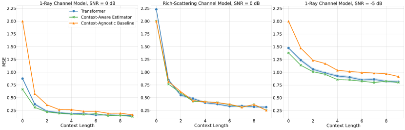
Figure 3: Results for Scenario C1, SNR = 0, -5 dB

Let us first discuss the 1-ray context. Here, even with zero context (pilots), the transformer model is able to perform better than the context-agnostic model. This indicates that the model is able to use the statistics of the ${\mathbf{y}}$ vectors to distinguish between 1-ray and rich-scattering data. As the context length increases, for both SNR values, the transformer model performs better than the context-agnostic baseline and approaches the performance of the lower-bound genie estimate. This shows that the model is able to determine the latent context and make a good estimate of the channel parameters, without being given any information beyond the $({\mathbf{y}},{\mathbf{x}})$ pairs themselves.

In the rich-scattering context, the three methods perform roughly the same across both SNR values and all context lengths. This is to be expected. The channel in this case is Gaussian with Gaussian noise, and simply estimating the mean and variance of the channel will grant the best performance. The notable aspect of this is that the transformer model is able to correctly identify the context and has learned the correct way to estimate the channel for this context.

VI-B Scenario C2: Estimation on a Time-Varying Channel

We trained a GPT-2 model as described previously on data sampled from scenario C2. We present results for this scenario in Figure 4. The plot here is produced similarly to Figure 3 with the added challenge that the channel coefficients vary with the index $k$.

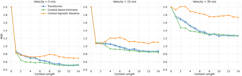
Figure 4: Results for Scenario C2, SNR = 0 dB

In Figure 4, we can see that the transformer model and both estimators have an MSE of 2.0 for zero context at every velocity. This is to be expected, as an MSE of 2.0 indicates that the model is "hedging" by returning a value of 0, rather than predicting -1 or 1. Because the Gaussian noise ${\mathbf{z}}$ is negative or positive with equal probability, any model requires at least one $({\mathbf{y}},{\mathbf{x}})$ pair before it is able to make a meaningful prediction. Across all velocity values, the transformer model’s performance approaches the performance of the context-aware estimator as the context length increases. This indicates that with enough context, the model is able to estimate the latent context and the channel coefficients, even though those channel coefficients are changing over time. There is a significant gap between the performance of the context-agnostic baseline method and the performance of the two other methods, demonstrating that performing well on this problem requires knowing or estimating the velocity. The transformer model is able to accurately infer the context and use this information to perform nearly as well as the genie-aided context-aware estimator.

VI-C Discussion

Across the various tasks, parameters, and regimes studied, transformer models are able to infer the context from a few samples and then use this information to make an accurate estimation of the channel coefficients. We use genie-aided context-aware estimators to find lower bounds on the performance of any such model. These estimators are given exact, noiseless information about the context, which is not available to the transformer model. Even without such extra information, the transformer models we trained are able to approach and reach the performance of the context-aware methods. This finding demonstrates that the ability of transformers to learn in-context from prompts enables these models to perform well on wireless communication problems.

VII Conclusion

Prior work has shown that transformer models are able to perform in-context learning and that this ability can be applied to solve a large variety of problems. This work shows that the in-context learning setting translates directly to problems in wireless communication and that transformer models can be trained to perform estimation in this domain. The communication problems described here are difficult, and existing methods for solving them require significant knowledge of the problem setting. For example, the context-aware estimators which we use as lower bounds on estimation performance require exact knowledge of the current context, which is not readily available in practice.

Through empirical case studies, we have demonstrated that transformer models can achieve similarly good performance without prior knowledge by being trained on data from the relevant distribution. Other than these training samples, we do not give our transformer models any prior knowledge about the problem setting, even the fact that there are finitely many different contexts. The transformer models we trained have inferred details of the distribution from training samples and have learned to condition their outputs on the predicted context in a Bayesian manner. This surprising ability indicates that transformer models can reduce the information required to achieve state-of-the-art results across a variety of problems.

-A Detailed Derivation of Baseline and Context-Aware Estimators

Following Section V-A, we derive the exact expressions for the context-aware and the baseline estimators. First, we describe some notations. For ${\bm{a}}\in{\mathbb{C}}^{d}$, denote its real and imaginary parts as ${\bm{a}}_{I},{\bm{a}}_{Q}\in{\mathbb{R}}^{d}$ respectively, and its real vector representation (also, by abuse of notation) as ${\bm{a}}=[{\bm{a}}_{I}^{T}~{}{\bm{a}}_{Q}^{T}]^{T}\in\mathbb{R}^{2d}$. For $a\in{\mathbb{C}}$, define $T^{d}(a)\triangleq\begin{bmatrix}a_{I}&-a_{Q}\\ a_{Q}&a_{I}\end{bmatrix}\otimes{\bm{I}}_{d}\in\mathbb{R}^{2d\times 2d}$, where $\otimes$ denotes the Kronecker product. Observe that the real-valued matrix equation corresponding to 4 is given by

$${\mathbf{y}}_{t}={\mathbf{X}}_{t}{\mathbf{h}}_{t}(\theta)+{\mathbf{z}}_{t},\quad t\in[\ell],$$

where ${\mathbf{y}}_{t}=\begin{bmatrix}{\mathbf{y}}_{t,I}\\ {\mathbf{y}}_{t,Q}\end{bmatrix}\in\mathbb{R}^{2d},{\mathbf{X}}_{t}=T^{d}({\textnormal{x}}_{t})\in\mathbb{R}^{2d\times 2d},{\mathbf{z}}_{t}=\begin{bmatrix}{\mathbf{z}}_{t,I}\\ {\mathbf{z}}_{t,Q}\end{bmatrix}\in\mathbb{R}^{2d},{\mathbf{h}}_{t}(\theta)=\begin{bmatrix}{\mathbf{h}}_{t,I}(\theta)\\ {\mathbf{h}}_{t,Q}(\theta)\end{bmatrix}\in\mathbb{R}^{2d}$. For $k\in[\ell-1]$, we can define

$$\bar{{\mathbf{y}}}_{k}=\bar{{\mathbf{X}}}_{k}\bar{{\mathbf{h}}}_{k}(\theta)+\bar{{\mathbf{z}}}_{k},$$ (5)

where $\bar{{\mathbf{X}}}_{k}={\rm diag}({\mathbf{X}}_{1},{\mathbf{X}}_{2},\dots,{\mathbf{X}}_{k})\in\mathbb{R}^{2dk\times 2dk}$, $\bar{{\mathbf{y}}}_{k}=[{\mathbf{y}}_{1}^{T}~{}{\mathbf{y}}_{2}^{T}~{}\dots~{}{\mathbf{y}}_{k}^{T}]^{T}\in\mathbb{R}^{2dk}$ and similarly for $\bar{{\mathbf{h}}}_{k}(\theta),\bar{{\mathbf{z}}}_{k}$.

In the scenario C1, since ${\mathbf{h}}_{t}(\theta)={\mathbf{h}}_{1}(\theta)$ for all $t\in[\ell]$, we can rewrite 5 as

$$\bar{{\mathbf{y}}}_{k}=\tilde{{\mathbf{X}}}_{k}{\mathbf{h}}_{1}(\theta)+\bar{{\mathbf{z}}}_{k},$$ (6)

where $\tilde{{\mathbf{X}}}_{k}=[{\mathbf{X}}_{1}^{T}~{}{\mathbf{X}}_{2}^{T}~{}\dots~{}{\mathbf{X}}_{k}^{T}]^{T}\in{\mathbb{R}}^{2dk\times 2d}$.

-A1 Context-aware estimators

In this subsection, we describe the context-aware genie-estimators that achieve low MSE when the latent context $\theta$ is known, whose MSE serves as a lower bound on the achievable MSE for a context-agnostic estimator.

For $\theta=0$ in C1, we can evaluate the integral in the conditional expectation $\mathbb{E}[{\textnormal{x}}_{k+1}\mid S_{k},{\mathbf{y}}_{k+1},\theta=0]$ explicitly as follows

$$\mathbb{E}[{\textnormal{x}}_{k+1}\mid S_{k},{\mathbf{y}}_{k+1},\theta=0]=\sum_{a\in{\mathbb{S}}}aP({\textnormal{x}}_{k+1}=a\mid S_{k},{\mathbf{y}}_{k+1},\theta=0).$$ (7)

Denoting $\bar{q}_{0}(a)=P({\textnormal{x}}_{k+1}=a\mid S_{k},{\mathbf{y}}_{k+1},\theta=0)$, we can write that

$$\bar{q}_{0}(a) =P({\textnormal{x}}_{k+1}=a\mid S_{k},{\mathbf{y}}_{k+1},\theta=0)$$

$$=\frac{1}{C_{1}}P(a)P(S_{k},{\mathbf{y}}_{k+1}\mid a,\theta=0)$$

$$=\frac{1}{C_{1}}P(a)\int_{\alpha=0}^{\infty}P(S_{k},{\mathbf{y}}_{k+1},{\mathbf{h}}_{1}(0)=\bm{\phi}(\alpha)\mid a)d\alpha$$

$$=\frac{1}{C_{2}}P(a)\int_{\alpha=0}^{\infty}P({\mathbf{y}}_{k+1}\mid T^{d}(a),{\mathbf{h}}_{1}(0)=\bm{\phi}(\alpha))\prod_{t=1}^{k}P({\mathbf{y}}_{t}\mid{\mathbf{X}}_{t},{\mathbf{h}}_{1}(0)=\bm{\phi}(\alpha))d\alpha$$

$$=\frac{1}{C_{3}}P(a)\int_{\alpha=0}^{\infty}\exp(-||{\mathbf{y}}_{k+1}-T^{d}(a)\bm{\phi}(\alpha)||^{2}/(2\sigma^{2}))\prod_{t=1}^{k}\exp(-||{\mathbf{y}}_{t}-{\mathbf{X}}_{t}\bm{\phi}(\alpha)||^{2}/(2\sigma^{2}))d\alpha$$

$$=\frac{1}{C_{3}}\underbrace{P(a)\int_{\alpha=0}^{\infty}\exp\Big{(}-\frac{1}{2\sigma^{2}}\Big{(}||{\mathbf{y}}_{k+1}-T^{d}(a)\bm{\phi}(\alpha)||^{2}+\sum_{t=1}^{k}||{\mathbf{y}}_{t}-{\mathbf{X}}_{t}\bm{\phi}(\alpha)||^{2})\Big{)}\Big{)}d\alpha}_{q_{0}(a)},$$

where $C_{1},C_{2},C_{3}$ are constants independent of $a$, and $C_{3}=\sum_{a\in{\mathbb{S}}}q_{0}(a)$. Therefore, we have

$$\mathbb{E}[{\textnormal{x}}_{k+1}\mid S_{k},{\mathbf{y}}_{k+1},\theta=0]=\sum_{a\in{\mathbb{S}}}a\bar{q}_{0}(a)=\frac{\sum_{a\in{\mathbb{S}}}aq_{0}(a)}{\sum_{a\in{\mathbb{S}}}q_{0}(a)}.$$ (8)

Therefore, in the scenario C1, $\theta=0$, the mean squared error (MSE) achieved by the above estimator is the lower bound for any other estimator for ${\textnormal{x}}_{k+1}$ that is given only $S_{k}$ (and also $\theta$). In other cases, the explicit design of estimators that achieve the lowest MSE is infeasible due to a high dimensional integral. Hence instead, we design a context-aware genie-estimator that achieves a reasonably low MSE as an estimator given $S_{k},\theta$. Therefore, the emphasis is on how quickly the posterior on the the latent parameter concentrates by the set of in-context examples $S_{k}$. The context-aware estimator computes the Linear Minimum Mean Square Estimate (LMMSE) $\hat{{\bm{h}}}_{k+1}^{\rm LMMSE,\theta}$ for the channel parameter ${\mathbf{h}}_{k+1}(\theta)$ given the pilots $S_{k}$ and the latent context $\theta$. From Equations (5), (6), we can compute the LMMSE (Theorem 12.1, [27]) estimates for the channel given the context $\theta$ as

$$({\rm C1})~{}\hat{{\bm{h}}}_{1}^{\rm LMMSE,\theta} =\mathbb{E}[{\mathbf{h}}_{1}(\theta)]+{\bm{R}}_{h_{1},\tilde{Y}_{k}}^{\theta}({\bm{R}}_{\tilde{Y}_{k}}^{\theta})^{-1}\bar{{\mathbf{y}}}_{k}$$ (9)

$$({\rm C2})~{}\hat{{\bm{h}}}_{k+1}^{\rm LMMSE,\theta} ={\bm{R}}_{h_{k+1},Y_{k}}^{\theta}({\bm{R}}_{X_{k}}^{\theta})^{-1}\bar{{\mathbf{y}}}_{k},$$ (10)

where ${\bm{R}}^{\theta}_{h_{1},\tilde{Y}_{k}}=\mathbb{E}[\bar{{\mathbf{y}}}_{k}\bar{{\mathbf{y}}}_{k}^{T}],{\bm{R}}^{\theta}_{h_{1},\tilde{Y}_{k}}=\mathbb{E}[{\mathbf{h}}_{1}(\theta)\bar{{\mathbf{y}}}_{k}^{T}]$ from 6, and ${\bm{R}}^{\theta}_{h_{k+1},{Y}_{k}}=\mathbb{E}[\bar{{\mathbf{y}}}_{k}\bar{{\mathbf{y}}}_{k}^{T}],{\bm{R}}^{\theta}_{h_{k+1},{Y}_{k}}=\mathbb{E}[{\mathbf{h}}_{k+1}(\theta)\bar{{\mathbf{y}}}_{k}^{T}]$ from 5. Note that $\mathbb{E}[\bar{{\mathbf{y}}}_{k}]=\mathbf{0}_{2dk}$ since $\mathbb{E}[\bar{{\mathbf{X}}}_{k}]=\mathbf{0}_{2dk\times 2dk}$, and $\mathbb{E}[{\mathbf{h}}_{k+1}(\theta)]=0$ for any $\theta$ in C2. Observe that since $\bar{{\mathbf{y}}}_{k}$ and ${{\mathbf{h}}}_{k+1}(\theta)$ are jointly Gaussian conditioned on $\theta$, the estimate for the channel parameter ${\mathbf{h}}_{k+1}$ given $S_{k},\theta$ is in fact the minimum mean squared error (MMSE) estimate. Next, we give the expressions for the above correlation matrices.

For $\theta=0$, the mean and auto-correlation function can be computed as $\bm{\mu}_{h_{1}}^{0}=\mathbb{E}[{\mathbf{h}}_{1}(0)]=\frac{1}{\pi}\int_{\alpha=0}^{\pi}\bm{\phi}(\alpha)d\alpha$, and ${\bm{R}}^{0}_{h_{1}}=\mathbb{E}[{\mathbf{h}}_{1}(0){\mathbf{h}}_{1}^{T}(0)]=\frac{1}{\pi}\int_{\alpha=0}^{\pi}\bm{\phi}(\alpha)\bm{\phi}^{T}(\alpha)d\alpha$. For $\theta=1$, the mean and the auto-correlation function for ${\mathbf{h}}_{1}(1)$ are given by $\bm{\mu}^{1}_{h_{1}}=\mathbf{0}\in{\mathbb{R}}^{2d}$, and ${\bm{R}}^{1}_{h_{1}}=\mathbb{E}[{\mathbf{h}}_{1}(1){\mathbf{h}}_{1}(1)^{T}]=\frac{1}{2}{\bm{I}}_{2d}$ respectively. Further, the auto-correlation of $\bar{{\mathbf{y}}}_{k}$ is given by ${\bm{R}}^{\theta}_{X_{k}}=\tilde{{\mathbf{X}}}_{k}{\bm{R}}_{h_{1}}^{\theta}\tilde{{\mathbf{X}}}_{k}^{T}+\sigma^{2}{\bm{I}}_{2dk}$, and the cross-correlation matrix is given by ${\bm{R}}_{h_{1},X_{k}}^{\theta}={\bm{R}}_{h_{1}}^{\theta}\tilde{{\mathbf{X}}}_{k}^{T}$.

In C2, the auto-correlation of channel parameter variables under the latent context $\theta$ is given by ${\bm{R}}^{\theta}_{H_{k}^{d}}=\mathbb{E}[\bar{{\mathbf{h}}}_{k}(\theta)\bar{{\mathbf{h}}}_{k}^{T}(\theta)]={\bm{R}}_{H_{k}}^{\theta}\otimes{\bm{I}}_{d}$, where $({\bm{R}}_{H_{k}}^{\theta})_{i,j}=R_{\theta}(|i-j|)$. Further, the cross correlation between $\bar{{\mathbf{y}}}_{k}$ and ${\mathbf{h}}_{k+1}$ is given by ${\bm{R}}_{h_{k+1},Y_{k}}^{\theta}=\mathbb{E}[{\mathbf{h}}_{k+1}\bar{{\mathbf{y}}}_{k}^{T}]={\bm{R}}_{h_{k+1},H^{d}_{k}}^{\theta}\bar{{\mathbf{X}}}_{k}^{T}$, where ${\bm{R}}^{\theta}_{h_{k+1},H_{k}^{d}}=[R_{\theta}(k)~{}R_{\theta}(k-1)~{}\dots~{}R_{\theta}(1)]\otimes{\bm{I}}_{2d}\in{\mathbb{R}}^{2d\times 2dk}$. Finally, the auto-correlation of $\bar{{\mathbf{y}}}_{k}$ is given by ${\bm{R}}^{\theta}_{Y_{k}}=\bar{{\mathbf{X}}}_{k}{\bm{R}}^{\theta}_{H_{k}^{d}}\bar{{\mathbf{X}}}_{k}^{T}+\sigma^{2}{\bm{I}}_{2dk}$.

After computing $\hat{{\bm{h}}}_{k+1}^{\rm LMMSE,\theta}$ using Equations (9), (10) the estimator computes the posterior mean estimate for symbol ${\textnormal{x}}_{k+1}$ as $\hat{{\textnormal{x}}}_{k+1}=\mathbb{E}[{\textnormal{x}}_{k+1}\mid{\mathbf{h}}_{k+1}(\theta)=\hat{{\bm{h}}}_{k+1}^{\rm LMMSE,\theta},{\mathbf{y}}_{k+1}]=\sum_{a\in{\mathbb{S}}}aP_{x}({\textnormal{x}}_{k+1}=a\mid\hat{{\bm{h}}}_{k+1}^{\rm LMMSE,\theta},{\mathbf{y}}_{k+1})$. Simplifying, we have

$$\bar{q}_{\bm{h}}(a)\triangleq P({\textnormal{x}}_{k+1}=a\mid{\mathbf{h}}_{k+1}(\theta)={\bm{h}},{\mathbf{y}}_{k+1}) =\frac{1}{C_{1}}P(a)P({\mathbf{y}}_{k+1}\mid{\mathbf{h}}_{k+1}(\theta)={\bm{h}},a)$$

$$=\frac{1}{C_{2}}\underbrace{P(a)\exp(-(||{\mathbf{y}}_{k+1}-T^{d}(a){\bm{h}})||^{2}/(2\sigma^{2})))}_{q_{\bm{h}}(a)},$$

where $C_{1},C_{2}$ are constants independent of $a$. Since $C_{2}=\sum_{a\in{\mathbb{S}}}q_{{\bm{h}}}(a)$, we have that the symbol estimate is

$$\hat{{\textnormal{x}}}_{k+1}=\sum_{a\in{\mathbb{S}}}\bar{q}_{\hat{{\bm{h}}}_{k+1}^{\rm LMMSE,\theta}}(a)=\frac{\sum_{a\in{\mathbb{S}}}aq_{\hat{{\bm{h}}}_{k+1}^{\rm LMMSE,\theta}}(a)}{\sum_{a\in{\mathbb{S}}}q_{\hat{{\bm{h}}}_{k+1}^{\rm LMMSE,\theta}}(a)}.$$ (11)

-A2 Baseline for context-agnostic estimators

Traditional signal processing techniques cannot use the hierarchical structure of the prior on the channel. We design a baseline which first computes the LMMSE for the channel parameter as

$$\hat{{\bm{h}}}_{k+1}^{\rm LMMSE}=\mathbb{E}[{\mathbf{h}}_{k+1}]+{\bm{R}}_{h_{k+1},Y_{k}}{\bm{R}}_{Y_{k}}^{-1}\bar{{\mathbf{y}}}_{k}.$$ (12)

Notice that since the above estimator does not have the information about the latent context $\theta$, we use the true correlation matrices on the joint prior of on the process $({\mathbf{h}}_{t})$, given by ${\bm{R}}_{Y_{k}}=\sum_{\theta\in\Theta}P_{\Theta}(\theta){\bm{R}}^{\theta}_{Y_{k}}$, ${\bm{R}}_{h_{k+1},Y_{k}}=\sum_{\theta\in\Theta}P_{\Theta}(\theta){\bm{R}}^{\theta}_{h_{k+1},Y_{k}}$, and $\mathbb{E}[{\mathbf{h}}_{k+1}]=\sum_{\theta\in\Theta}P_{\Theta}(\theta)\mathbb{E}[{\mathbf{h}}_{k+1}(\theta)]$. Finally, we estimate the symbol ${\textnormal{x}}_{k+1}$ using 11 with $q_{\hat{{\bm{h}}}_{k+1}^{\rm LMMSE,\theta}}$ is replaced by $q_{\hat{{\bm{h}}}_{k+1}^{\rm LMMSE}}$.

-B Model Parameters

We extend the codebase from [2] for our models and experiments. We use the same GPT-2 model size as in this paper, as well as the same optimizer (Adam, [28]), the same learning rate (0.0001), and the same training length (500,000 steps).

Embedding Size	# Layers	# Attention Heads
256	12	8

TABLE I: Model Parameters

Scenario	Curriculum Start Length	Curr. End Length	Batch Size	Learning Rate
C1	5	11	64	1e-4
C2	5	15	64	1e-4

TABLE II: Training Parameters

Curriculum: [1] observed that curriculum learning is useful in training models to perform in-context learning consistently and effectively. In [1] and [2], the curriculum is to initiate training with small sequence lengths and vector dimensions and to increase these gradually over training until they reach the desired sizes. In our tasks, the vector dimension is fixed to twice the number of antennae, and we modify only the sequence lengths in our curriculum. For scenario C1, we vary the sequence length from 5 to a maximum of 11. For scenario C2, we vary the sequence length from 5 to a maximum of 15. We choose to use a larger sequence length for scenario C2 in order to better demonstrate the impact of using a time-varying channel.

We present the relevant architecture details and training parameters in Tables I and II.

References

- [1] Shivam Garg, Dimitris Tsipras, Percy Liang, and Gregory Valiant, “What can transformers learn in-context? a case study of simple function classes,” 2023.
- [2] Kabir Ahuja, Madhur Panwar, and Navin Goyal, “In-context learning through the bayesian prism,” 2023.
- [3] Ashish Vaswani, Noam Shazeer, Niki Parmar, Jakob Uszkoreit, Llion Jones, Aidan N Gomez, Ł ukasz Kaiser, and Illia Polosukhin, “Attention is all you need,” in Advances in Neural Information Processing Systems, I. Guyon, U. Von Luxburg, S. Bengio, H. Wallach, R. Fergus, S. Vishwanathan, and R. Garnett, Eds. 2017, vol. 30, Curran Associates, Inc.
- [4] Tom B. Brown, Benjamin Mann, Nick Ryder, Melanie Subbiah, Jared Kaplan, Prafulla Dhariwal, Arvind Neelakantan, Pranav Shyam, Girish Sastry, Amanda Askell, Sandhini Agarwal, Ariel Herbert-Voss, Gretchen Krueger, Tom Henighan, Rewon Child, Aditya Ramesh, Daniel M. Ziegler, Jeffrey Wu, Clemens Winter, Christopher Hesse, Mark Chen, Eric Sigler, Mateusz Litwin, Scott Gray, Benjamin Chess, Jack Clark, Christopher Berner, Sam McCandlish, Alec Radford, Ilya Sutskever, and Dario Amodei, “Language models are few-shot learners,” in Proceedings of the 34th International Conference on Neural Information Processing Systems, Red Hook, NY, USA, 2020, NIPS’20, Curran Associates Inc.
- [5] Sang Michael Xie, Aditi Raghunathan, Percy Liang, and Tengyu Ma, “An explanation of in-context learning as implicit bayesian inference,” in International Conference on Learning Representations, 2022.
- [6] Arvind Mahankali, Tatsunori B. Hashimoto, and Tengyu Ma, “One step of gradient descent is provably the optimal in-context learner with one layer of linear self-attention,” 2023.
- [7] Ruiqi Zhang, Spencer Frei, and Peter L. Bartlett, “Trained transformers learn linear models in-context,” ArXiv, vol. abs/2306.09927, 2023.
- [8] Ekin Akyürek, Dale Schuurmans, Jacob Andreas, Tengyu Ma, and Denny Zhou, “What learning algorithm is in-context learning? investigations with linear models,” in The Eleventh International Conference on Learning Representations, 2023.
- [9] Johannes Von Oswald, Eyvind Niklasson, Ettore Randazzo, João Sacramento, Alexander Mordvintsev, Andrey Zhmoginov, and Max Vladymyrov, “Transformers learn in-context by gradient descent,” in International Conference on Machine Learning. PMLR, 2023, pp. 35151–35174.
- [10] Kwangjun Ahn, Xiang Cheng, Hadi Daneshmand, and Suvrit Sra, “Transformers learn to implement preconditioned gradient descent for in-context learning,” arXiv preprint arXiv:2306.00297, 2023.
- [11] Stephanie Chan, Adam Santoro, Andrew Lampinen, Jane Wang, Aaditya Singh, Pierre Richemond, James McClelland, and Felix Hill, “Data distributional properties drive emergent in-context learning in transformers,” in Advances in Neural Information Processing Systems, S. Koyejo, S. Mohamed, A. Agarwal, D. Belgrave, K. Cho, and A. Oh, Eds. 2022, vol. 35, pp. 18878–18891, Curran Associates, Inc.
- [12] Sewon Min, Xinxi Lyu, Ari Holtzman, Mikel Artetxe, Mike Lewis, Hannaneh Hajishirzi, and Luke Zettlemoyer, “Rethinking the role of demonstrations: What makes in-context learning work?,” in Proceedings of the 2022 Conference on Empirical Methods in Natural Language Processing, 2022, pp. 11048–11064.
- [13] Michael Baur, Benedikt Fesl, Michael Koller, and Wolfgang Utschick, “Variational autoencoder leveraged MMSE channel estimation,” in 2022 56th Asilomar Conference on Signals, Systems, and Computers, 2022, pp. 527–532.
- [14] Avi Caciularu and David Burshtein, “Unsupervised linear and nonlinear channel equalization and decoding using variational autoencoders,” IEEE Transactions on Cognitive Communications and Networking, vol. 6, no. 3, pp. 1003–1018, 2020.
- [15] An Le Ha, Trinh Van Chien, Tien Hoa Nguyen, Wan Choi, and Van Duc Nguyen, “Deep learning-aided 5G channel estimation,” in 2021 15th International Conference on Ubiquitous Information Management and Communication (IMCOM), 2021, pp. 1–7.
- [16] David Neumann, Thomas Wiese, and Wolfgang Utschick, “Learning the MMSE channel estimator,” IEEE Transactions on Signal Processing, vol. 66, no. 11, pp. 2905–2917, 2018.
- [17] Chao Lu, Wei Xu, Hong Shen, Jun Zhu, and Kezhi Wang, “MIMO channel information feedback using deep recurrent network,” IEEE Communications Letters, vol. 23, no. 1, pp. 188–191, 2019.
- [18] Fayçal Ait Aoudia and Jakob Hoydis, “End-to-end learning for ofdm: From neural receivers to pilotless communication,” IEEE Transactions on Wireless Communications, vol. 21, no. 2, pp. 1049–1063, 2021.
- [19] Fayçal Ait Aoudia and Jakob Hoydis, “End-to-end learning for ofdm: From neural receivers to pilotless communication,” IEEE Transactions on Wireless Communications, vol. 21, no. 2, pp. 1049–1063, 2022.
- [20] David Neumann, Thomas Wiese, and Wolfgang Utschick, “Learning the mmse channel estimator,” IEEE Transactions on Signal Processing, vol. 66, no. 11, pp. 2905–2917, 2018.
- [21] Avi Caciularu and David Burshtein, “Unsupervised linear and nonlinear channel equalization and decoding using variational autoencoders,” IEEE Transactions on Cognitive Communications and Networking, vol. 6, no. 3, pp. 1003–1018, 2020.
- [22] David Burshtein and Eli Bery, “Semi-supervised variational inference over nonlinear channels,” 2023.
- [23] Tianqi Wang, Chao-Kai Wen, Shi Jin, and Geoffrey Ye Li, “Deep learning-based csi feedback approach for time-varying massive mimo channels,” IEEE Wireless Communications Letters, vol. 8, no. 2, pp. 416–419, 2019.
- [24] Ruiqi Zhang, Spencer Frei, and Peter L. Bartlett, “Trained transformers learn linear models in-context,” 2023.
- [25] Vanya Cohen and Aaron Gokaslan, “Opengpt-2: Open language models and implications of generated text,” XRDS, vol. 27, no. 1, pp. 26–30, sep 2020.
- [26] Andrea Goldsmith, Wireless Communications, Cambridge University Press, 2005.
- [27] S. M. Kay, Fundamentals of Statistical Signal Processing: Estimation Theory, Prentice Hall, 1997.
- [28] Diederik P. Kingma and Jimmy Ba, “Adam: A method for stochastic optimization,” CoRR, vol. abs/1412.6980, 2014.