Distributed Task Allocation for Self-Interested Agents with Partially Unknown Rewards

Abstract

This paper provides a novel solution to a task allocation problem, by which a group of agents decides on the assignment of a discrete set of tasks in a distributed manner. In this setting, heterogeneous agents have individual preferences and associated rewards for doing each task; however, these rewards are only known asymptotically. We start by formulating the assignment problem by means of a combinatorial partition game for known rewards, with no constraints on number of tasks per agent. We relax this into a weight game, which together with the former, are shown to contain the optimal task allocation in the corresponding set of Nash Equilibria (NE). We then propose a projected, best-response, ascending gradient dynamics (PBRAG) that converges to a NE in finite time. This forms the basis of a distributed online version that can deal with a converging sequence of rewards by means of an agreement sub-routine. We present simulations that support our results.

1 Introduction

A prototypical multi-agent coordination problem aims to find an efficient assignment of group of agents to complete a collection of tasks. These tasks can range from abstract sets of objectives to specific physical jobs, the nature of which may not be completely known. In addition, the agents composing the group may have heterogeneous capabilities, and react to different sets of incentives that are being learned progressively. This necessitates of novel task-assignment algorithms that can adapt and react online as new information arises. Motivated by this, we study a discrete task allocation problem modeled as a game of self-interested agents that have partial knowledge of their rewards. This requires addressing the problem’s combinatorial nature, and designing provable-correct distributed dynamics that adapt to dynamic rewards revealed online. To the best of our knowledge, algorithms that combine all these features are not available in literature.

Literature review

The problem of task allocation with known rewards has been widely considered; see e.g. [1, 2, 3]. A centralized solution to this problem, where the number $m$ of tasks and agents are equal and a task-agent matching is sought, is the optimization-based Hungarian algorithm [4], and its distributed version [5]. The latter, which reproduces the Hungarian algorithm locally, requires tracking of the agents’ identities associated with each task, has a time complexity of $O(m^{3})$ and communication cost of $O(m\log m)$ (per communication round). Thus, the algorithm can be computationally and memory-intensive for large problems, and hard to adapt as new tasks are generated or their valuations change online. The work in [6] provides a tractable, sub-optimal solution to the same NP-hard problem, while the research in [7] showed that the sub-optimality can be resolved by restricting heterogeneous agents to be of certain types. In the same vein, the works in [8, 9, 10] considers submodular functions which allow rewards to take any non-negative value. However, submodular optimization can be applied in specific domains where the property naturally arises, such as in certain economics and distributed sensing problems. Alternatively, a well known approach to (unconstrained) task assignment problems is given by $k$-means clustering and the Lloyd’s algorithm [11]. By interpreting that tasks are generated by a probability distribution, the approach can handle tasks generated dynamically [12, 13, 14, 15]. However, it is well known that Lloyd’s algorithm is sensitive to the initial task assignment for a small number of agents, and converges to a local minima.

Game-theoretic models have also been proposed to find solutions to task allocation problems. For sensor networks, each agent is equipped with an appropriate utility function [16, 17, 18] and the optimal task allocation is related to the Nash equilibrium of this game. Any Nash-seeking [19] algorithm returns a solution; but often, these algorithms require strong assumptions on the utility functions and their derivatives. Distributed versions of Nash-seeking with consensus in continuous time have been explored in [20, 21], while [22, 23] addressed the problem in discrete time. All the work in [20]-[23] assumed complete and perfect information for agents, while in practice, agents may have limited or imperfect information about the tasks, and the capabilities of other agents. Potential games can be used in this regards, but they do not work when the reward parameters are unknown. To that end, [18] characterizes transient behavior for set covering games, and [24] looks at a general potential game approach for task allocation. In the latter case, the agents are homogeneous and tasks have same rewards for all agents.

Contributions

We consider a task-assignment problem where a number of agents is to be matched to an unrestricted set of tasks. In the considered formulation, the number of tasks per agent is not constrained, yet the optimal assignment problem remains combinatorial as the number of tasks is discrete. To deal with arbitrary heteregenous agents, we derive a game-theoretic partition problem formulation that favors task distribution. We then relax the game into a weight game, one per task. We obtain characterizations of the NE of each game, their relationship, and identify conditions under which the NE leads to an optimal solution of the original assignment problem. Leveraging the relaxed formulation, and under a full-information assumption, we derive a projected best-response dynamics that is shown to converge to the optimal task allocation in finite time. This forms the basis for a new algorithm, PBRAG, which is distributed, does not require the knowledge of other agent identities, and converges to the optimal task allocation, also in finite time, as rewards are revealed online.

2 Preliminaries

Here, we formalize the notations and briefly list some well-known concepts that are used to solve the problem formulated in the following section.

2-A Notations

The sets of real numbers, non-negative real numbers, and non-negative integers are denoted as $\mathbb{R}$, $\mathbb{R}_{\geq 0}$, and $\mathbb{Z}_{\geq 0}$, respectively. For a set $\mathcal{S}$, $|\mathcal{S}|$ denotes its cardinality, $2^{\mathcal{S}}$ represents the class of all its subsets, $\mathcal{S}^{n}$ denotes the $n$ Cartesian product of $\mathcal{S}$ with itself, and $\mathcal{S}^{n\times m}$ collects all $n\times m$ matrices whose $(i,j)^{\text{th}}$ entry lies in $\mathcal{S}$. Given $\mathbf{M}\in\mathcal{S}^{n\times m}$, $m^{j}_{i}$ is its $(i,j)^{\text{th}}$ entry, and $\mathbf{m}_{i}^{\top}\in\mathcal{S}^{m}$ (resp. $\mathbf{m}^{j}\in\mathcal{S}^{n}$) its $i^{\text{th}}$ row (resp. its $j^{\text{th}}$ column). For $x\in\mathbb{R}$, $[x]_{0}^{1}:=\max\{0,\min\{x,1\}\}$. For a set $\mathcal{S}$, define $\operatorname*{max^{(2)}}\mathcal{S}:=\max\{s\in\mathcal{S}\,|\,s\neq\max\,\mathcal{S}\}$. For a vector $\mathbf{x}\in\mathbb{R}^{n}$ and a set $\mathcal{S}\subseteq\mathbb{R}^{n}$, $d(\mathbf{x},\mathcal{S}):=\inf_{\mathbf{y}\in\mathcal{S}}\|\mathbf{x}-\mathbf{y}\|_{1}$ is the distance of the vector from the set. Lastly, the empty set is denoted as $\varnothing$.

2-B Game theory

A strategic form game [25] is a tuple $\mathscr{G}:=\left<\mathcal{A},\{\mathcal{S}_{i}\}_{i\in\mathcal{A}},\{\psi_{i}\}_{i\in\mathcal{A}}\right>$ consisting of the following components:

1. a set of players (or agents) $\mathcal{A}$;

2. a set of strategies $s_{i}\in\mathcal{S}_{i}$ available to each $i\in\mathcal{A}$;

3. a set of utility functions $\psi_{i}:\times_{i\in\mathcal{A}}\mathcal{S}_{i}\to\mathbb{R}$ over the strategy profiles of all the agents.

In what follows, $s_{-i}$ denotes the strategy profile of all players other than $i\in\mathcal{A}$. Next, we formally state the definition of the NE of a strategic form game.

Definition 2.1 (Nash equilibrium).

The strategy profile $(\widehat{s}_{i},\widehat{s}_{-i})$ is a Nash equilibrium (NE) of $\mathscr{G}$ if and only if

$$\psi_{i}(\widehat{s}_{i},\widehat{s}_{-i})\geq\psi_{i}(s_{i},\widehat{s}_{-i}),\,\,\forall s_{i}\in\mathcal{S}_{i},\,\,\forall i\in\mathcal{A}\,.$$

$\mathcal{NE}(\mathscr{G})$ denotes the set of all Nash equilibria of $\mathscr{G}$. $\bullet$

2-C Graph theory

A directed graph [26] $\mathcal{G}:=(\mathcal{A},\mathcal{E})$, is a tuple consisting of (a) a set of nodes (here agents $\mathcal{A}$); (b) a set of arcs $\mathcal{E}\subseteq\mathcal{A}\times\mathcal{A}$ between the nodes. The set $\mathcal{N}_{i}:=\{j\in\mathcal{A}\,|\,(j,i)\in\mathcal{E}\}$ denotes the (in) neighbors of node $i\in\mathcal{A}$ and $\overline{\mathcal{N}}_{i}:=\mathcal{N}_{i}\cup\{i\}$. A path is an ordered set of non-repeating nodes such that each tuple of adjacent nodes belongs to $\mathcal{E}$. The graph $\mathcal{G}$ is said to be strongly connected if there exists a path from every node to every other node. The diameter of the graph $\mathrm{diam}(\mathcal{G})$ is the length of the largest possible path between any two nodes.

3 Problem Formulation

A group of agents $\mathcal{A}:=\{1,\cdots,n\}$ is to complete a set of tasks $\mathcal{Q}:=\{1,\cdots,m\}$, where $n\neq m$ possibly, in a distributed manner. For this purpose, each agent $i\in\mathcal{A}$ encodes via $\phi_{i}:\mathcal{Q}\to\mathbb{R}_{\geq 0}$ the importance of each task (the higher $\phi_{i}(q)$ the larger the agent’s capability/fondness on $q\in\mathcal{Q}$) and $r_{i}:\mathcal{Q}\to\mathbb{R}_{\geq 0}$ the reward for completing each task. For the sake of brevity, define $f_{i}(q):=r_{i}(q)\phi_{i}(q)\geq 0$, $\forall q\in\mathcal{Q}$, $\forall i\in\mathcal{A}$. An optimal task assignment is the solution to

$$\max_{{\mathcal{P}=(\mathcal{V}_{1},\cdots,\mathcal{V}_{n})\subseteq\mathcal{Q}^{n}}}\quad J(\mathcal{P}):=\sum_{i\in\mathcal{A}}\sum_{q\in\mathcal{V}_{i}}f_{i}(q),$$ (1a)

$$\mathrm{s.t.}\quad\bigcup_{i\in\mathcal{A}}\mathcal{V}_{i}=\mathcal{Q};\quad\mathcal{V}_{i}\cap\mathcal{V}_{j}=\varnothing,\,\,\mathrm{if}\,\,i\neq j.$$ (1b)

Here, $\mathcal{V}_{i}\subseteq\mathcal{Q}$ is the set of tasks assigned to agent $i\in\mathcal{A}$ and $\mathcal{P}=(\mathcal{V}_{1},\cdots,\mathcal{V}_{n})$ is the ordered collection of sets that defines a partition of $\mathcal{Q}$ (as in 1b).

The group of agents is to compute an optimal partition of the task set $\mathcal{Q}$ on their own. Naturally, each agent $i\in\mathcal{A}$ aims to get the tasks $q\in\mathcal{Q}$ for which $f_{i}(q)$ is the largest. This motivates the following definition.

Definition 3.1 (Task specific dominating agent).

An agent $i\in\mathcal{A}$ is said to be a dominating agent for task $q\in\mathcal{Q}$ (or $i$ is dominating for $q$), if $f_{i}(q)\geq f_{j}(q)$, $\forall j\in\mathcal{A}$. If a task $q\in\mathcal{Q}$ has exactly one dominating agent, we say that there exists a unique dominating agent for task $q$. $\bullet$

The collection of possible strategies for each agent is a combinatorial class, which grows exponentially as the number of tasks $m$ increases. To address this problem, we first assume that each $i\in\mathcal{A}$ measures the utility of a subset of tasks $\mathcal{V}_{i}\subseteq\mathcal{Q}$ via

$$H_{i}(\mathcal{V}_{i},\mathcal{V}_{-i}):=\sum_{q\in\mathcal{V}_{i}}\Big{[}f_{i}(q)-\max_{j\in\mathcal{A}\setminus\{i\},q\in\mathcal{V}_{j}}f_{j}(q)\Big{]}.$$ (2)

This leads to the partition game

$$\mathscr{G}_{P}:={\left<\mathcal{A},\{2^{\mathcal{Q}}\}_{i\in\mathcal{A}},\{H_{i}\}_{i\in\mathcal{A}}\right>},$$

where the strategy of each agent is to choose a subset $\mathcal{V}_{i}$ of $\mathcal{Q}$ to maximize $H_{i}$. In this way, agent strategies are no-longer required to form a valid partition, but the utility in 2 penalizes each agent for taking tasks that others have chosen.

Second, we further relax this game by reducing the decision of each agent $i\in\mathcal{A}$ regarding task $q\in\mathcal{Q}$ to the computation of a weight $w^{q}_{i}\in[0,1]$. Briefly, this defines $\mathbf{W}\in[0,1]^{n\times m}$ as the matrix whose $(i,q)^{\text{th}}$ entry is $w^{q}_{i}$. Thus, $\mathbf{w}_{i}^{\top}\in[0,1]^{m}$ (resp. $\mathbf{w}^{q}\in[0,1]^{n}$) represents the weights that agent $i\in\mathcal{A}$ (resp. for task $q\in\mathcal{Q}$) gives to each task (resp. given by each agent). Agent $i\in\mathcal{A}$ is equipped with the utility function:

$$U_{i}(\mathbf{w}_{i},\mathbf{w}_{-i}) =\sum_{q\in\mathcal{Q}}\Big{[}f_{i}(q)w^{q}_{i}-\max_{j\in\mathcal{A}\setminus\{i\}}f_{j}(q)w^{q}_{j}w^{q}_{i}\Big{]}\,,$$ (3)

which collectively define the weight game

$$\mathscr{G}_{W}:={\left<\mathcal{A},\mathbf{W},\{U_{i}\}_{i\in\mathcal{A}}\right>},$$

In this way, a product of weights in the second part of the sum in 3 relaxes the check on overlapping task in 2. In this paper, we ignore the trivial case where all agents get the same payoff for a task, as stated in the following.

Assumption 3.2 (Non-trivial task assignment).

Not all agents are dominating for each task $q\in\mathcal{Q}$. $\bullet$

The above framework allows us to deal with a case where the $f_{i}(q)$ are unknown to the agent, but where these values can be learned progressively by an external mechanism until convergence. More precisely, we assume the following.

Assumption 3.3 (Converging reward sequence).

For each $i\in\mathcal{A}$, $q\in\mathcal{Q}$, there exists a sequence $\{z^{q}_{i}(t)\}_{t\in\mathbb{Z}_{\geq 0}}$ such that $z^{q}_{i}(t)\to f_{i}(q)$ as $t\to\infty$. $\bullet$

In what follows, we first study the games when the reward parameters are known. Then we adapt the results for the case when only a converging reward sequence is available.

Now we formally state the goals of this work.

Problem 3.4.

Given the aforementioned setup and the non-trivial task assignment assumption, find

1. a relationship between the NE of $\mathscr{G}_{P}$ and $\mathscr{G}_{W}$,

2. a relationship between the NE and optimal partitions according to 1,

3. a distributed algorithm that converges to the NE of the limiting weight game $\mathscr{G}_{W}$ under the converging reward sequence assumption. $\bullet$

4 On Nash Equilibria and Optimal Partitions

We start by addressing the first two problems above. Thus, we first characterize the NE of the partition game $\mathscr{G}_{P}$.

Lemma 4.1 (Nash equilibria of $\mathscr{G}_{P}$).

The strategy $(\widehat{\mathcal{V}}_{i},\widehat{\mathcal{V}}_{-i})\in\mathcal{NE}(\mathscr{G}_{P})$ if and only if:

1. for each $q\in\mathcal{Q}$, $\exists\,i\in\mathcal{A}$ dominating for $q$ and $q\in\widehat{\mathcal{V}}_{i}$;

2. if $j$ is not a dominating agent for task $q$, then $q\not\in\widehat{\mathcal{V}}_{j}$.

Proof. First, we show the necessity of Properties 1 and 2. Suppose that $(\widehat{\mathcal{V}}_{i},\widehat{\mathcal{V}}_{-i})\in\mathcal{NE}(\mathscr{G}_{P})$. We prove Property 1 by contradiction and assume $\exists\,q\in\mathcal{Q}$ such that $\forall i\in\mathcal{A}$ dominating for task $q$, $q\notin\widehat{\mathcal{V}}_{i}$. Pick one such agent $i$ and take $\mathcal{V}_{i}=\widehat{\mathcal{V}}_{i}\cup\{q\}$. Then,

$$H_{i}(\mathcal{V}_{i},\widehat{\mathcal{V}}_{-i})-H_{i}(\widehat{\mathcal{V}}_{i},\widehat{\mathcal{V}}_{-i})=f_{i}(q)-\max_{k\neq i,\,q\in\widehat{\mathcal{V}}_{k}}f_{k}(q)>0.$$

The inequality is strict since $i$ is dominating and the max is over all agents that are not dominating for $q$ (by assumption). This is a contradiction with $(\widehat{\mathcal{V}}_{i},\widehat{\mathcal{V}}_{-i})\in\mathcal{NE}(\mathscr{G}_{P})$.

The necessity of Property 2 also follows from contradiction. Suppose $\exists\,q\in\mathcal{Q}$ and a $j\in\mathcal{A}$ not dominating for $q$ with $q\in\widehat{\mathcal{V}}_{j}$. From Property 1, there is an $i\in\mathcal{A}$ dominating for $q$ with $q\in\widehat{\mathcal{V}}_{i}$. Thus, with strategy $(\widehat{\mathcal{V}}_{j},\widehat{\mathcal{V}}_{-j})$,

$$f_{j}(q)-\max_{k\neq j,\,q\in\widehat{\mathcal{V}}_{k}}f_{k}(q)=f_{j}(q)-\max_{k\in\mathcal{A}}f_{k}(q)<0.$$

Now, consider the strategy $\mathcal{V}_{j}=\widehat{\mathcal{V}}_{j}\setminus\{q\}$. It follows that $H_{j}(\mathcal{V}_{j},\widehat{\mathcal{V}}_{-j})-H_{j}(\widehat{\mathcal{V}}_{j},\widehat{\mathcal{V}}_{-j})>0$, which contradicts $(\widehat{\mathcal{V}}_{j},\widehat{\mathcal{V}}_{-j})\in\mathcal{NE}(\mathscr{G}_{P})$.

Now, we show the sufficiency of Properties 1 and 2. Let $(\widehat{\mathcal{V}}_{i},\widehat{\mathcal{V}}_{-i})$ satisfy Properties 1 and 2 and let $i\in\mathcal{A}$ be an arbitrary but fixed agent. Suppose that $\mathcal{V}_{i}\neq\widehat{\mathcal{V}}_{i}$ is any other strategy. Then, the proof follows from three cases:

Case (i): $\exists\,q\in\mathcal{V}_{i}$ such that $q\notin\widehat{\mathcal{V}}_{i}$ and $i$ is dominating for $q$. Then, since $\exists\,j\in\mathcal{A}$ dominating for $q$ with $q\in\widehat{\mathcal{V}}_{j}$,

$$f_{i}(q)-\max_{k\neq i,\,q\in\widehat{\mathcal{V}}_{k}}f_{k}(q)=f_{i}(q)-f_{j}(q)=0.$$

Case (ii): $\exists\,q\in\mathcal{V}_{i}$ such that $q\notin\widehat{\mathcal{V}}_{i}$ and $i$ does not dominate $q$. Then, as $\exists\,j\in\mathcal{A}$ dominating for $q$ and $q\in\widehat{\mathcal{V}}_{j}$, we have

$$f_{i}(q)-\max_{k\neq i,\,q\in\widehat{\mathcal{V}}_{k}}f_{k}(q)=f_{i}(q)-f_{j}(q)<0.$$

Case (iii): $\exists\,q\in\widehat{\mathcal{V}}_{i}$ such that $q\notin\mathcal{V}_{i}$. This can only happen if $i$ is dominating for $q$ (else, by Property 2, $q\notin\widehat{\mathcal{V}}_{j}$). Then,

$$f_{i}(q)-\max_{k\neq i,\,q\in\widehat{\mathcal{V}}_{k}}f_{k}(q)\geq 0.$$

From the above, it is easy to see that any deviation from $(\widehat{\mathcal{V}}_{i},\widehat{\mathcal{V}}_{-i})$ will not result in an increase in utility for $i$ since $H_{i}(\mathcal{V}_{i},\widehat{\mathcal{V}}_{-i})-H_{i}(\widehat{\mathcal{V}}_{i},\widehat{\mathcal{V}}_{-i})=f_{i}(q)-\max\limits_{k\neq i,\,q\in\widehat{\mathcal{V}}_{k}}f_{k}(q)$. $\blacksquare$

From the previous result, at least one of the dominating agents will be assigned to a task by means of a NE strategy of $\mathscr{G}_{P}$. However, this does not preclude that two dominating agents are assigned the same task. Next, we show that the NE of the relaxed game $\mathscr{G}_{W}$ are equivalent to the NE of $\mathscr{G}_{P}$.

Lemma 4.2 (Nash equilibria of $\mathscr{G}_{W}$).

The strategy $(\widehat{\mathbf{w}}_{i},\widehat{\mathbf{w}}_{-i})\in\mathcal{NE}(\mathscr{G}_{W})$ if and only if:

1. for each $q\in\mathcal{Q}$, $\exists\,i\in\mathcal{A}$ dominating for $q$ and $\widehat{w}^{q}_{i}=1$;

2. if $j$ is not a dominating agent for task $q$, then $\widehat{w}^{q}_{j}=0$.

Proof. First, we show the necessity of all properties. Suppose $(\widehat{\mathbf{w}}_{i},\widehat{\mathbf{w}}_{-i})\in\mathcal{NE}(\mathscr{G}_{W})$. We show Property 1 is necessary by contradiction. Consider an arbitrary $q\in\mathcal{Q}$ and suppose that for all dominating agents $i^{*}_{q}\in\mathcal{A}$ for task $q$, it holds that $\widehat{w}^{q}_{i^{*}_{q}}<1$. In particular, for any such $i^{*}_{q}$, we have $\max_{j\neq\{i^{*}_{q}\}}f_{j}(q)\widehat{w}^{q}_{j}<f_{i^{*}_{q}}(q)$. Now consider the strategy $\mathbf{w}_{i^{*}_{q}}$, where $w^{q}_{i^{*}_{q}}=1$ and $w^{i^{*}_{q}}_{p}=\widehat{w}^{i^{*}_{q}}_{p}$, $\forall p\neq q\in\mathcal{Q}$. Then,

$$U_{i^{*}_{q}}(\mathbf{w}_{i^{*}_{q}},\widehat{\mathbf{w}}_{-i^{*}_{q}})-U_{i^{*}_{q}}(\widehat{\mathbf{w}}_{i^{*}_{q}},\widehat{\mathbf{w}}_{-i^{*}_{q}})=$$

$$\hskip 30.00005pt\Big{[}f_{i^{*}_{q}}(q)-\max_{j\neq i^{*}_{q}}f_{j}(q)\widehat{w}^{q}_{j}\Big{]}\big{[}1-\widehat{w}^{q}_{i^{*}_{q}}\big{]}>0.$$

This leads to a contradiction with $(\widehat{\mathbf{w}}_{i},\widehat{\mathbf{w}}_{-i})\in\mathcal{NE}(\mathscr{G}_{W})$.

We similarly show Property 2 is necessary by contradiction. Let $q\in\mathcal{Q}$ be an arbitrary task, and suppose that $\exists\,j\in\mathcal{A}$ which is not dominating for $q$ but for which $\widehat{w}^{q}_{j}>0$. Due to Property 1, let $i^{*}_{q}$ be the dominating agent for $q$ such that $\widehat{w}^{q}_{i^{*}_{q}}=1$. Now define a new strategy $\mathbf{w}_{j}$, with $w^{q}_{j}=0$ and $w^{j}_{p}=\widehat{w}^{j}_{p}$, $\forall p\neq q\in\mathcal{Q}$. Then,

$$U_{j}(\mathbf{w}_{j},\widehat{\mathbf{w}}_{-j})-U_{j}(\widehat{\mathbf{w}}_{j},\widehat{\mathbf{w}}_{-j})=\big{[}f_{j}(q)-f_{i^{*}_{q}}(q)\big{]}[-\widehat{w}^{q}_{j}]>0,$$

where the inequality is because both terms are negative. This contradicts $(\widehat{\mathbf{w}}_{i},\widehat{\mathbf{w}}_{-i})\in\mathcal{NE}(\mathscr{G}_{W})$.

Next, we show sufficiency. Let $(\widehat{\mathbf{w}}_{i},\widehat{\mathbf{w}}_{-i})\in[0,1]^{n\times m}$ be a candidate strategy satisfying Properties 1- 2 and let $i\in\mathcal{A}$. Take any other $\mathbf{w}_{i}\neq\widehat{\mathbf{w}}_{i}$ and a task $q\in\mathcal{Q}$. The proof follows from the following cases.

Case (i): $i$ is a dominating agent for task $q$ and $\widehat{w}^{q}_{i}=1$. Then, from Definition 3.1,

$$\Big{[}f_{i}(q)-\max_{j\neq i}f_{j}(q)\widehat{w}^{q}_{j}\Big{]}w^{q}_{i}\leq\Big{[}f_{i}(q)-\max_{j\neq i}f_{j}(q)\widehat{w}^{q}_{j}\Big{]}\widehat{w}^{q}_{i}.$$

Case (ii): $i$ is a dominating agent for task $q$ and ${\widehat{w}^{q}_{i}<1}$. Then, since $\exists\,j\in\mathcal{A}$ dominating for $q$ and $\widehat{w}^{q}_{j}=1$,

$$\Big{[}f_{i}(q)-\max_{k\neq i}f_{k}(q)\widehat{w}^{q}_{k}\Big{]}w^{q}_{i}=\big{[}f_{i}(q)-f_{j}(q)\big{]}w^{q}_{i}$$

$$=\big{[}f_{i}(q)-f_{j}(q)\big{]}\widehat{w}^{q}_{i}=\Big{[}f_{i}(q)-\max_{k\neq i}f_{k}(q)\widehat{w}^{q}_{k}\Big{]}\widehat{w}^{q}_{i}=0,$$

since $f_{i}(q)-f_{j}(q)=0$.

Case (iii): $i$ is not a dominating agent for task $q$ (and hence $\widehat{w}^{q}_{i}=0$). Again, $\exists\,j\in\mathcal{A}$ dominating for $q$ and $\widehat{w}^{q}_{j}=1$. Then,

$$\Big{[}f_{i}(q)-\max_{k\neq i}f_{k}(q)\widehat{w}^{q}_{k}\Big{]}w^{q}_{i}=\big{[}f_{i}(q)-f_{j}(q)\big{]}w^{q}_{i}$$

$$<\big{[}f_{i}(q)-f_{j}(q)\big{]}\widehat{w}^{q}_{i}=\Big{[}f_{i}(q)-\max_{k\neq i}f_{k}(q)\widehat{w}^{q}_{k}\Big{]}\widehat{w}^{q}_{i},$$

since $f_{i}(q)<f_{j}(q)$. Now, using these three cases, it is easy to see that any deviation from $(\widehat{\mathbf{w}}_{i},\widehat{\mathbf{w}}_{-i})$ will not result in an increase the utility of $i$. $\blacksquare$

As a direct implication of Lemma 4.2, for any $\mathbf{W}\in[0,1]^{n\times m}$ we can define $C:[0,1]^{n\times m}\to(2^{\mathcal{Q}})^{n}$ as

$$C(\mathbf{W}):=(\mathrm{tsupp}\,(\mathbf{w}_{1}),\cdots,\mathrm{tsupp}\,(\mathbf{w}_{n})),$$ (4)

where $\mathrm{tsupp}\,(\mathbf{w}_{i}):=\{q\in\mathcal{Q}\,|\,w^{q}_{i}=1\},\,\,\forall i\in\mathcal{A}$. Then,

$$\mathcal{NE}(\mathscr{G}_{P})=C(\mathcal{NE}(\mathscr{G}_{W})).$$ (5)

Next, we relate the optimal partition and the NE of the two games through the following theorem.

Theorem 4.3 (Optimal partitions and Nash equilibria).

Given the problem in 1 , $\mathcal{O}\subseteq C(\mathcal{NE}(\mathscr{G}_{W}))$, where

$$\mathcal{O}:=\{\mathcal{P}^{*}\,\,|\,\,\mathcal{P}^{*}\,\,\mathrm{is\,\,a\,\,solution\,\,to\,\,}\lx@cref{refnum}{eq:partition_optimization}\}.$$ (6)

Proof. By 5, we can equivalently show that $\mathcal{O}\subseteq\mathcal{NE}(\mathscr{G}_{P})$. Let $\mathcal{P}^{*}\in\mathcal{O}$. It is easy to see that $q\in\mathcal{V}^{*}_{i}$ only if $i\in\mathcal{A}$ is a dominating agent for task $q$. Moreover, if $j\in\mathcal{A}$ is not dominating for $q$, then $q\notin\mathcal{V}^{*}_{j}$. Then from Lemma 4.1, $\mathcal{P}^{*}\in\mathcal{NE}(\mathscr{G}_{P})$. The rest follows from 5. $\blacksquare$

The above result states that if an agent $i\in\mathcal{A}$ is assigned tasks using the translated support of the NE of $\mathscr{G}_{W}$, this set is a superset of the optimizers of 1. The extra solutions arise when there are non-unique dominating agents for a task. When there are unique dominating agents, the next result shows there is a unique NE for $\mathscr{G}_{W}$. This follows from Lemma 4.2 immediately, so we skip a formal proof.

Corollary 4.4 (Uniqueness of Nash equilibria).

Suppose that for each $q\in\mathcal{Q}$, $i^{*}_{q}$ is the unique dominating agent for task $q$. Then $\mathcal{NE}(\mathscr{G}_{W})=\{\widehat{\mathbf{W}}\}$ where, for each $q\in\mathcal{Q}$, $\widehat{\mathbf{W}}$ satisfies 1) $\widehat{w}^{q}_{i^{*}_{q}}=1$, and 2) $\widehat{w}^{q}_{j}=0$, $\forall\,j\neq i^{*}_{q}$. Further, $\mathcal{P}^{*}=C(\widehat{\mathbf{W}})$ is the unique solution to 1. $\blacksquare$

In general, $\mathcal{NE}(\mathscr{G}_{W})$ is a superset of the set of optimal partitions. The next example makes this clear.

Example 4.5 (Optimal partitions and Nash equilibria).

Let $\mathcal{A}=\{1,2\}$ and $\mathcal{Q}=\{\mathfrak{a},\mathfrak{b}\}$. Assume the values $f_{1}(\mathfrak{a})=f_{2}(\mathfrak{a})=0.5$, $f_{1}(\mathfrak{b})=0.7$ and $f_{2}(\mathfrak{b})=0.3$. Then, $\mathcal{O}=\{(\{\mathfrak{a},\mathfrak{b}\},\varnothing),(\{\mathfrak{b}\},\{\mathfrak{a}\})\}$; $\mathcal{NE}(\mathscr{G}_{P})=\{(\{\mathfrak{a},\mathfrak{b}\},\varnothing),(\{\mathfrak{a},\mathfrak{b}\},\{\mathfrak{a}\}),(\{\mathfrak{b}\},\{\mathfrak{a}\})\}$; and

$$\mathcal{NE}(\mathscr{G}_{W})=\left\{\begin{bmatrix}1&1\\ \lambda&0\end{bmatrix},\begin{bmatrix}1&1\\ 1&0\end{bmatrix},\begin{bmatrix}\mu&1\\ 1&0\end{bmatrix}\right\},$$

where $\lambda,\mu$ can independently take any value in $[0,1)$. Thus, in this case $\mathcal{O}\subsetneq\mathcal{NE}(\mathscr{G}_{P})=C(\mathcal{NE}(\mathscr{G}_{W}))$. Interestingly, note that there is an optimal partition in which agent $2$ does not get any task. $\bullet$

Next, we design a dynamical system using which the agents can figure out the optimal partition on their own.

5 Best Response Projected Gradient Ascent

From the previous section, we know that if the agents play the weight game $\mathscr{G}_{W}$, then the NE form a superset of the optimal task partition (with slight abuse of notation). Thus, here we let the agents update their weights (from any initial feasible weight) using the gradient of their utility while assuming the others do not change their weights. For such a dynamical system, we aim to relate its equilibria to the NE of $\mathscr{G}_{W}$ and hence also relate it to the set $\mathcal{O}$ of optimal solutions to 1. Now, from 3, it can be seen that,

$$\frac{\partial}{\partial w^{q}_{i}}U_{i}=f_{i}(q)-\max_{j\in\mathcal{A}\setminus\{i\}}f_{j}(q)w^{q}_{j}\,=:u^{q}_{i}(\mathbf{w}^{q})\,.$$ (7)

Thus, the weights are updated using the following dynamics:

$$w^{q}_{i}(t+1)=\big{[}w^{q}_{i}(t)+\gamma^{q}_{i}\,u^{q}_{i}(\mathbf{w}^{q}(t))\big{]}_{0}^{1},$$ (8)

with $\gamma^{q}_{i}\in\mathbb{R}_{>0}$, $\forall i\in\mathcal{A},\forall q\in\mathcal{Q}$. We call this the projected best response ascending gradient dynamics (PBRAG). From 7 and 8, note that in order to compute the weight updates, each agent $i\in\mathcal{A}$ needs to know $f_{j}(q)w^{q}_{j}$, for all $j\neq i$. This requires that each agent must talk to every other agent to compute its own gradient. The equilibrium points of this dynamics is given by

$$\mathcal{W}:=\Big{\{}\mathbf{W}\in[0,1]^{n\times m}\ \vline\ \Big{[}w^{q}_{i}+\gamma^{q}_{i}\,u^{q}_{i}(\mathbf{w}^{q})\Big{]}_{0}^{1}=w^{q}_{i},$$

$$\hskip 150.00023pt\forall i\in\mathcal{A},\forall q\in\mathcal{Q}\Big{\}}.$$ (9)

For this, the following result can be stated immediately.

Lemma 5.1 (Equilibrium weights are Nash equilibria).

The weight matrix $\overline{\mathbf{W}}\in\mathcal{W}$ if and only if $\overline{\mathbf{W}}\in\mathcal{NE}(\mathscr{G}_{W})$.

Proof. We prove this by showing that $\overline{\mathbf{W}}\in\mathcal{W}$ if and only if $\overline{\mathbf{W}}$ follows Properties 1 and 2 of Lemma 4.2. Suppose that $\overline{\mathbf{W}}\in\mathcal{W}$ and consider an arbitrary but fixed $q\in\mathcal{Q}$. We prove Property 1 by contradiction and assume that $\forall i\in\mathcal{A}$ dominating for $q$, $\overline{w}^{q}_{i}<1$. Now, for any dominating agent $i^{*}_{q}\in\mathcal{A}$, $\max_{j\in\mathcal{A}\setminus\{i^{*}_{q}\}}f_{j}(q)\overline{w}^{q}_{j}<f_{i^{*}_{q}}(q)$. Thus, $u^{q}_{i^{*}_{q}}(\overline{\mathbf{w}}^{q})>0$. Since $\overline{w}^{q}_{i^{*}_{q}}<1$ and $\gamma^{q}_{i^{*}_{q}}>0$, this contradicts $\overline{\mathbf{W}}\in\mathcal{W}$.

Next we prove Property 2 also by contradiction. Suppose that $\exists\,j\in\mathcal{A}$ not dominating for task $q$ but $\overline{w}^{q}_{j}>0$. Due to Property 1, let $i^{*}_{q}\in\mathcal{A}$ be the dominating agent for task $q$ such that $\overline{w}^{q}_{i^{*}_{q}}=1$. Then,

$$u^{q}_{j}(\overline{\mathbf{w}}^{q})=f_{j}(q)-\max_{k\in\mathcal{A}\setminus\{j\}}f_{k}(q)\overline{w}^{q}_{k}=f_{j}(q)-f_{i^{*}_{q}}(q)<0\,.$$

Again, as $\overline{w}^{q}_{j}>0$ and $\gamma^{q}_{j}>0$, this contradicts $\overline{\mathbf{W}}\in\mathcal{W}$.

To show sufficiency, let $\overline{\mathbf{W}}$ satisfy Properties 1 and 2. Then it is easy to see that for each task $q\in\mathcal{Q}$, $u^{q}_{i}(\overline{\mathbf{w}}^{q})\geq 0$ if $i\in\mathcal{A}$ is dominating for $q$ with $\overline{w}^{q}_{i}=1$, $u^{q}_{i}(\overline{\mathbf{w}}^{q})=0$ if $i\in\mathcal{A}$ is dominating for $q$ with $\overline{w}^{q}_{i}<1$, and $u^{q}_{j}(\overline{\mathbf{w}}^{q})<0$ if $j\in\mathcal{A}$ is not dominating for $q$ (hence $\overline{w}^{q}_{j}=0$). Then, $\overline{\mathbf{W}}\in\mathcal{W}$ follows since $\gamma^{q}_{j}>0$. $\blacksquare$

From Lemma 5.1, we can also infer that if there is a unique dominating agent, then the equilibrium set becomes a singleton and follows the same structure as in Corollary 4.4.

In what follows, we show that starting from any initial weights, the dynamics 8 converges to an equilibrium.

Theorem 5.2 (PBRAG  converges to an equilibrium weight).

Suppose Assumption 3.2 holds. Consider the dynamics 8 with an initial condition $\mathbf{W}(0)\in[0,1]^{n\times m}$ and let $\mathbf{W}(t)$ be the solution trajectory. Then $\lim_{t\to\infty}\mathbf{W}(t)=\overline{\mathbf{W}}\in\mathcal{W}$.

Proof. Notice that for the dynamics 8, the weight associated with each task evolves independently from the weights associated with other tasks. Thus, consider an arbitrary but fixed $q\in\mathcal{Q}$. Next, consider any $i\in\mathcal{A}$ that is dominating for $q$. From 7, $u^{q}_{i}(\mathbf{w}^{q})\geq 0$, $\forall\,\mathbf{w}^{q}\in[0,1]^{n}$. Thus, since $\gamma^{q}_{i}>0$, $\forall i\in\mathcal{A}$, $w^{q}_{i}(t)$ is non-decreasing. Hence, $w^{q}_{i}(t)\to\widehat{w}^{q}_{i}\in[0,1]$ as $t\to\infty$, since $[0,1]$ is compact. Now consider $\mathcal{I}^{q}:=\{j\in\mathcal{A}\,|\,j\,\,\mathrm{is\,\,dominating\,\,for}\,\,q\}$, the set $\mathcal{X}:=\{\mathbf{v}\in[0,1]^{|\mathcal{I}^{q}|}\,|\,v_{j}=1\,\,\mathrm{for\,\,some}\,\,j\in\mathcal{I}^{q}\}$ and define the continuous function $V(\mathbf{w}^{q}):=d(\{w^{q}_{i}\}_{i\in\mathcal{I}^{q}},\mathcal{X})$. It is clear that $V(\mathbf{w}^{q}(t+1))\leq V(\mathbf{w}^{q}(t))$ $\forall t\in\mathbb{Z}_{\geq 0}$. Applying the LaSalle invariance principle, there is convergence to the largest invariant set in $V(\mathbf{w}(t))=V(\mathbf{w}(t+1))$ for all $t$. We argue this set is necessarily $\mathcal{X}$. Otherwise, invariance implies that $u^{q}_{i}(\mathbf{w}^{q})=0$ for any dominating agent $i\in\mathcal{A}$. However, this occurs if and only if $\exists\,i^{\prime}\in\mathcal{A}$, $i\neq i^{\prime}$, another dominating agent for task $q$ such that $w^{q}_{i^{\prime}}=1$; otherwise, $u^{q}_{i}(\mathbf{w}^{q})>0$. Thus, $\{w^{q}_{i}(t)\}_{i\in\mathcal{I}^{q}}\to\mathcal{X}$ as $t\to\infty$ . This along with previous discussion proves that $\widehat{w}^{q}_{i}$ follows Property 1 of Lemma 4.2.

Next consider any $j\in\mathcal{A}$ that is not dominating for $q$. From the previous part of the proof, we know that there is a $i\in\mathcal{A}$ dominating for $q$ for which $w^{q}_{i}(t)\to 1$ and thus $f_{i}(q)w^{q}_{i}(t)\to f_{i}(q)$ as $t\to\infty$. This implies that $\exists\,\tau\in\mathbb{Z}_{\geq 0}$ such that $\max_{k\in\mathcal{A}\setminus\{j\}}f_{k}(q)w^{q}_{k}(t)\geq f_{j}(q)+\nu$, for some $\nu>0$ and $\forall t\geq\tau$. Then, as $u^{q}_{j}(\mathbf{w}^{q}(t))\leq-\nu<0$, $w^{q}_{j}(t)$ is a strictly decreasing sequence (after $\tau$ time steps). Thus, from the dynamics in 8, $w^{q}_{j}(t)\to\widehat{w}^{q}_{j}=0$ as $t\to\infty$. Hence, $\widehat{w}^{q}_{j}$ follows Property 2 of Lemma 4.2. $\blacksquare$

When there is a unique dominating agent for each task, we can guarantee finite-time convergence to an optimal partition.

Theorem 5.3 (PBRAG  converges in finite time).

Suppose Assumption 3.2 holds and suppose that for each $q\in\mathcal{Q}$, there exists a unique dominating agent, $i_{q}^{*}\in\mathcal{A}$. Define $\gamma:=\min\limits_{i\in\mathcal{A},q\in\mathcal{Q}}\gamma^{q}_{i}>0$, and let $\delta:=\min\limits_{q\in\mathcal{Q}}\big{[}f_{i^{*}_{q}}(q)-\max\limits_{j\neq i^{*}_{q}}f_{j}(q)\big{]}>0$. Consider the dynamics 8 starting from $\mathbf{W}(0)\in[0,1]^{n\times m}$, with the solution trajectory $\mathbf{W}(t)\rightarrow\overline{\mathbf{W}}\in\mathcal{W}$, as $t\rightarrow\infty$. Then $w^{q}_{i}(t)=\overline{w}^{q}_{i}$, $\forall i\in\mathcal{A}$, $\forall q\in\mathcal{Q}$, $\forall t\geq 2\left\lceil(\gamma\delta)^{-1}\right\rceil$.

Proof. From Lemma 5.1 and Corollary 4.4, it is clear that $\mathcal{W}$ is a singleton set. Let $\overline{\mathbf{W}}\in\mathcal{W}$ be the unique equilibrium point. From Theorem 5.2, we know that $\mathbf{W}(t)\to\overline{\mathbf{W}}$ as $t\to\infty$. From 7, $u^{q}_{i^{*}_{q}}(\mathbf{w}^{q}(t))\geq\delta>0,\forall t\in\mathbb{Z}_{\geq 0}$ and hence from 8, $\forall t\in\mathbb{Z}_{\geq 0}$, $w^{q}_{i^{*}_{q}}(t+1)\geq[w^{q}_{i^{*}_{q}}(t)+\gamma^{q}_{i^{*}_{q}}\,\delta]_{0}^{1}\geq[w^{q}_{i^{*}_{q}}(0)+(t+1)\,\gamma^{q}_{i^{*}_{q}}\,\delta]_{0}^{1}$. The inequality holds since $[\cdot]_{0}^{1}$ is a nondecreasing function. Thus, $w^{q}_{i^{*}_{q}}(t)=1$, for all $t\geq\left\lceil(\gamma\delta)^{-1}\right\rceil\geq(\gamma\delta)^{-1}\geq[1-w^{q}_{i^{*}_{q}}(0)][\gamma^{q}_{i^{*}_{q}}\delta]^{-1}$. Now define $\tau:=\left\lceil(\gamma\delta)^{-1}\right\rceil$ and consider any $j\neq i^{*}_{q}$ and notice from 7 that $u^{q}_{j}(\mathbf{w}^{q}(t))\leq-\delta<0,\forall t\geq\tau$. Thus, $w^{q}_{j}(t)\leq[w^{q}_{j}(\tau)-t\,\gamma^{q}_{j}\,\delta]_{0}^{1},\forall t\geq\tau.$ The inequality again holds since $[\cdot]_{0}^{1}$ is non decreasing. So, $w^{q}_{j}(t)=0$, for all $t\geq\tau+\left\lceil(\gamma\delta)^{-1}\right\rceil\geq\tau+[\gamma^{q}_{j}\delta]^{-1}\geq\tau+w^{q}_{j}(\tau)[\gamma^{q}_{j}\delta]^{-1}$. $\blacksquare$

Remark 5.4 (On the effect of step-size on convergence).

By Theorem 5.2, 8 converges to an equilibrium weight when $\gamma^{q}_{i}>0$, $\forall i\in\mathcal{A}$, $\forall q\in\mathcal{Q}$. Thus agents can choose any constant positive step size and guarantee convergence to a NE of the weight game. Further inspection of Theorem 5.3 leads to this interesting observation. Since $\delta^{-1}>0$, the individual $\gamma^{q}_{i}$’s can be chosen in such a way that $0<{(\gamma\delta)}^{-1}<1$. Then $2\left\lceil(\gamma\delta)^{-1}\right\rceil=2$. That is, by choosing a sufficiently large step size and communicating with every other agent, the agents can reach the NE in at most two time steps. $\bullet$

In order to avoid all-to-all communication, it is possible to adapt 8 introducing a consensus subroutine. In the next section, we utilize this idea to handle decentralization together with unknown rewards.

6 Distributed Task Allocation

Here, we provide a solution to Problem 3.4 (3). Recall that in Section 5, each agent $i\in\mathcal{A}$ computes $\max_{j\neq i}f_{j}(q)w^{q}_{j}$ using information from all other agents. Here, we introduce a communication graph $\mathcal{G}:=(\mathcal{A},\mathcal{E})$ with vertex set $\mathcal{A}$. The arc set $\mathcal{E}$ defines the connections between agents, with $(i,j)\in\mathcal{E}$ if and only if $i\in\mathcal{A}$ can send information to $j\in\mathcal{A}$. For the sake of brevity, let $\mathrm{d}:=\mathrm{diam}(\mathcal{G})$.

For such a setup, the following result gives a way to find the max and second unique max values in a distributed fashion. This is useful in providing a distributed PBRAG (d-PBRAG).

Lemma 6.1 (Agreement on the two largest variables in a network).

Let $\mathcal{G}$ be a strongly connected graph and consider

$$M^{q}_{i}(t+1)=\max_{j\in\overline{\mathcal{N}}_{i}}M^{q}_{j}(t),$$ (10a)

$$S^{q}_{i}(t+1)=\operatorname*{max^{(2)}}\Big{\{}\{S^{q}_{j}(t)\}_{j\in\overline{\mathcal{N}}_{i}},M^{q}_{i}(t),v^{q}_{i}\Big{\}},$$ (10b)

with initial condition $M^{q}_{i}(0)=S^{q}_{i}(0)=v^{q}_{i}\in\mathbb{R}_{\geq 0}$, $\forall i\in\mathcal{A}$, $\forall q\in\mathcal{Q}$. Then $\forall\,q\in\mathcal{Q}$ and $\forall\,i\in\mathcal{A}$;

1. $M^{q}_{i}(t)=\max\{v^{q}_{j}\}_{j\in\mathcal{A}}$, $\forall\,t\geq\mathrm{d}$,

2. $S^{q}_{i}(t)=\operatorname*{max^{(2)}}\{v^{q}_{j}\}_{j\in\mathcal{A}}$, $\forall\,t\geq 2\,\mathrm{d}$.

Proof. We show this for an arbitrary but fixed $q\in\mathcal{Q}$. Let $i^{*}_{q}\in\operatorname*{argmax}\{v^{q}_{j}\}_{j\in\mathcal{A}}$. Then, from 10a, $M^{q}_{i^{*}_{q}}(t)=v^{q}_{i^{*}_{q}}$, $\forall t\in\mathbb{Z}_{\geq 0}$. Thus, $\forall\,i^{*}_{q}\in\operatorname*{argmax}\{v^{q}_{j}\}_{j\in\mathcal{A}}$, $M^{q}_{j}(t)=v^{q}_{i^{*}_{q}}$, $\forall j\in\mathcal{N}_{i^{*}_{q}}$, $\forall t\geq 1$. Continuing this argument inductively proves Property 1 since $\mathcal{G}$ is strongly connected.

To show Property 2, we use Property 1. Now let $i^{*}_{q}\in\operatorname*{argmax^{(2)}}\{v^{q}_{j}\}_{j\in\mathcal{A}}$. Then, from 10b, $S^{q}_{i^{*}_{q}}(t)=v^{q}_{i^{*}_{q}}$, $\forall t\geq\mathrm{d}$. Thus, similarly, $\forall\,i^{*}_{q}\in\operatorname*{argmax^{(2)}}\{v^{q}_{j}\}_{j\in\mathcal{A}}$, $S^{q}_{j}(t)=v^{q}_{i^{*}_{q}}$, $\forall j\in\mathcal{N}_{i^{*}_{q}}$, $\forall t\geq\mathrm{d}+1$. Again, continuing this argument proves Property 2 since $\mathcal{G}$ is strongly connected. $\blacksquare$

To compute the gradient and update the weights $w^{q}_{i}$ simultaneously, we propose the following dynamics:

$$w^{q}_{i}(t+1)=\Big{[}w^{q}_{i}(t)+\gamma^{q}_{i}(t)\Big{(}z^{q}_{i}(t)-\frac{1}{2}\big{(}M^{q}_{i}(t)+S^{q}_{i}(t)\big{)}\Big{)}\Big{]}_{0}^{1},$$ (11a)

$$M^{q}_{i}(t+1)=\sigma_{\mathrm{sw}}\Big{(}\max_{j\in\overline{\mathcal{N}}_{i}}M^{q}_{j}(t),e^{q}_{i}(t+1),t+1,T\Big{)},$$ (11b)

$$S^{q}_{i}(t+1)=\sigma_{\mathrm{sw}}\Big{(}\operatorname*{max^{(2)}}\Big{\{}\{S^{q}_{j}(t)\}_{j\in\overline{\mathcal{N}}_{i}},M^{q}_{i}(t),e^{q}_{i}(t)\Big{\}},$$

$$\hskip 120.00018pte^{q}_{i}(t+1),t+1,T\Big{)},$$ (11c)

$$e^{q}_{i}(t+1)=\sigma_{\mathrm{sw}}\Big{(}e^{q}_{i}(t),z^{q}_{i}(t+1),t+1,T\Big{)}\,,$$ (11d)

for some $T\in\mathbb{R}_{\geq 0}$ and where $\sigma_{\mathrm{sw}}$ is the switching function

$$\sigma_{\mathrm{sw}}\Big{(}m,z,t,T\Big{)}:=\begin{cases}z,&\mathrm{if}\,\,t\,\,\mathrm{mod}\,\,T=0,\\ m,&\mathrm{otherwise}\,.\end{cases}$$ (12)

Remark 6.2 (d-PBRAG  with agreement and periodic input injection).

Note that $\forall\,i\in\mathcal{A}$, $\forall\,q\in\mathcal{Q}$, the weight update in 11a uses the sequence $\{z^{q}_{i}(t)\}_{t\in\mathbb{Z}_{\geq 0}}$ and a time-varying step-size $\gamma^{q}_{i}(t)$ instead of $f_{i}(q)$ and a constant step-size $\gamma^{q}_{i}$; respectively, as in 8. The periodic switching function $\sigma_{\mathrm{sw}}$ ensures that $e^{q}_{i}(t)$ holds the value $z^{q}_{i}(t)$ for every $T$ time-steps. This in turn allows 11b and 11c to run an agreement subroutine as 10 every $T$ time-steps with $v^{q}_{i}=z^{q}_{i}(kT)$, for $k\in\mathbb{Z}_{\geq 0}$. Thus, at every time-step which is a multiple of $T$, each agent believes that its own value is the maximum and corrects this belief over the next $T-1$ time-steps. $\bullet$

Theorem 6.3 (Asymptotic behavior of d-PBRAG).

Suppose Assumptions 3.2 and 3.3 hold. Define

$$\Delta^{q}:=\Big{(}\max_{i\in\mathcal{A}}f_{i}(q)-\min_{i\in\mathcal{A}}f_{i}(q)\Big{)}>0,\,\forall q\in\mathcal{Q}\,.$$ (13)

Consider any $\varepsilon\in(0,1)$. Suppose $\forall t\in\mathbb{Z}_{\geq 0}$, $\gamma^{q}_{i}(t)=\alpha^{q}_{i}$, with $0<\alpha^{q}_{i}\leq\varepsilon\,(2\,\mathrm{d}\,\Delta^{q})^{-1}$, $\forall i\in\mathcal{A}$, $\forall q\in\mathcal{Q}$. Next, define $\alpha:=\min_{i\in\mathcal{A},q\in\mathcal{Q}}\alpha^{q}_{i}$, $\mu^{q}:=0.5\,(\max\{f_{i}(q)\}_{i\in\mathcal{A}}-\operatorname*{max^{(2)}}\{f_{i}(q)\}_{i\in\mathcal{A}})$, and

$$\mu:=(1-\nu)\min_{q\in\mathcal{Q}}\mu^{q}>0,$$ (14)

with $\nu\in(0,1)$. Further, suppose $T>2\,\mathrm{d}+(\alpha\,\mu)^{-1}+1$. Let $\mathbf{W}(t)$ be the solution trajectory to 11 starting from $\mathbf{W}(0)\in[0,1]^{n\times m}$. Then $\exists\,\tau(\mathbf{W}(0))\in\mathbb{Z}_{\geq 0}$ such that $\forall\,t\geq\tau$,

1. $w^{q}_{i}(t)=1$ if $i\in\mathcal{A}$ is dominating for $q\in\mathcal{Q}$;

2. $w^{q}_{j}(t)\leq\varepsilon$ if $j\in\mathcal{A}$ is not dominating for $q\in\mathcal{Q}$.

Thus $C(\mathbf{W}(t))$ converges in finite number of time steps.

Proof. First note that the bounds on $\alpha^{q}_{i}$’s and $T$ are valid because of Assumption 3.2. Then, we show the claims for an arbitrary but fixed $q\in\mathcal{Q}$.

Recall that because of Assumption 3.3, $\exists\,\tau_{0}\in\mathbb{Z}_{\geq 0}$ such that $\forall t,t^{\prime}\geq\tau_{0}$, $z^{q}_{i}(t)-0.5\,(z^{q}_{i}(t)+z^{q}_{j}(t^{\prime}))<\Delta^{q}$, $\forall\,i,j\in\mathcal{A}$. Moreover $\tau_{0}$ can be chosen such that $z^{q}_{i^{*}_{q}}(t)-0.5\,(z^{q}_{i^{*}_{q}}(t)+z^{q}_{j}(t^{\prime}))\geq(1-\nu)\,\mu^{q}>0$, for any $\nu\in(0,1)$, if $i^{*}_{q}\in\operatorname*{argmax}_{i\in\mathcal{A}}f_{i}(q)$ and $\forall j\in\mathcal{A}$ such that $j\notin\operatorname*{argmax}_{i\in\mathcal{A}}f_{i}(q)$.

Now consider any $i^{*}_{q}\in\operatorname*{argmax}_{i\in\mathcal{A}}f_{i}(q)$ and any $\nu\in(0,1)$. Then from Remark 6.2 and from the previous discussion, it is clear that, $\forall t\geq\tau_{0}$,

$$\alpha^{q}_{i^{*}_{q}}\big{(}z^{q}_{i^{*}_{q}}(t)-0.5\big{(}M^{q}_{i^{*}_{q}}(t)+S^{q}_{i^{*}_{q}}(t)\big{)}\big{)}\geq\alpha^{q}_{i}(1-\nu)\,\mu^{q}\geq\alpha^{q}_{i}\mu\,.$$

This proves Property 1 of this theorem as $\alpha^{q}_{i}\mu>0$.

Next consider any $j\notin\operatorname*{argmax}_{i\in\mathcal{A}}f_{i}(q)$. Note from Remark 6.2 that $\forall t\geq\tau_{0}$ such that $t\in\{kT+2\mathrm{d},\cdots,2kT-1\}$ for some $k\in\mathbb{Z}_{\geq 0}$, $w^{q}_{j}(t)$ strictly decreases, since,

$$z^{q}_{j}(t)-0.5(M^{q}_{j}(t)+S^{q}_{j}(t))\leq-(1-\nu)\mu^{q}<0\,.$$

Consider any $t\geq\tau_{0}$ such that $t\in\{kT+2\mathrm{d},\cdots,2kT-1\}$ with $k\in\mathbb{Z}_{\geq 0}$. Then, since $w^{q}_{j}(kT+2\mathrm{d}-1)\leq 1$,

$$w^{q}_{j}(t)\leq 1-((t\,\,\mathrm{mod}\,\,T)-2\mathrm{d})\alpha\mu,$$

and hence because of the bound on $T$, $w^{q}_{j}(2kT-1)=0$. Finally, consider any $t\geq\tau_{0}$ such that $t\in\{kT,\cdots,kT+2\mathrm{d}-1\}$ with $k\in\mathbb{Z}_{\geq 0}$. Then, since $w^{q}_{j}(kT-1)=0$ (from previous arguments), we have $w^{q}_{j}(t)\leq(t\,\,\mathrm{mod}\,\,T)\,\alpha^{q}_{i}\,\Delta^{q}$. Thus combining all these arguments proves Property 2.

The final claim follows from the previous ones and 4. $\blacksquare$

Note that the previous result does not guarantee that the weights converge. This stems from the fact that at periodic times, each agent believes that it gets the maximum reward for each task. Moreover, the previous result needs information about the limits of the converging sequences to provide bounds for the step sizes and the period of input injection. This can be avoided by allowing time-varying step sizes as stated next.

Theorem 6.4 (d-PBRAG  converges to Nash equilibrium).

Suppose Assumptions 3.2 and 3.3 hold. Let $\mathbf{W}(t)$ be the solution trajectory of 11 from $\mathbf{W}(0)\in[0,1]^{n\times m}$, with $T>2\,\mathrm{d}+1$ and $\forall i\in\mathcal{A}$, $\forall q\in\mathcal{Q}$,

$$\gamma^{q}_{i}(t)=\begin{cases}\alpha^{q}_{i}(k)>0,&\mathrm{if}\,t\in\{kT,\cdots,kT+2\mathrm{d}-1\},\\ \beta^{q}_{i}(k)>0,&\mathrm{if}\,t\in\{kT+2\mathrm{d},\cdots,2kT-1\},\end{cases}$$

with $k\in\mathbb{Z}_{\geq 0}$. Further, $\forall i\in\mathcal{A}$, $\forall q\in\mathcal{Q}$; take sequences $\alpha^{q}_{i}(k)\to 0$ as $k\to\infty$ and $\beta^{q}_{i}(k)\to\infty$ as $k\to\infty$. Then $\mathbf{W}(t)\to\overline{\mathbf{W}}\in\mathcal{NE}(\mathscr{G}_{W})$ as $t\to\infty$.

Proof. From hypothesis, $\forall\varepsilon>0$, $\exists\,K\in\mathbb{Z}_{\geq 0}$, such that $\forall t\in\{kT,\cdots,kT+2\mathrm{d}-1\}$, with $k\geq K$, $\alpha^{q}_{i}(t)\leq\varepsilon\,(2\,\mathrm{d}\,\Delta^{q})^{-1}$, with $\Delta^{q}$ as in 13. Moreover, $K$ can be chosen such that $\forall t\in\{kT+2\mathrm{d},\cdots,2kT-1\}$, with $k\geq K$, $T>2\mathrm{d}+((1-\nu)\mu\min_{i\in\mathcal{A},q\in\mathcal{Q}}\alpha^{q}_{i}\beta^{q}_{i}(t))^{-1}+1$ for any $\nu\in(0,1)$ and with $\mu$ as in 14. Then the claim of this result is a consequence of applying similar arguments as in the proof of Theorem 6.3 and using 5. $\blacksquare$

We conclude this section by discussing some interesting observations about the parameters in 11.

Remark 6.5 (On the implementation of d-PBRAG).

Note that even though $\mathrm{diam}(\mathcal{G})$ is an internal property of the communication graph $\mathcal{G}$ and requires some structural knowledge of the same, the claims in Theorems 6.3 and 6.4 remain true if $\mathrm{d}$ is replaced with $n$. This is because $\mathrm{diam}(\mathcal{G})\leq n$. Moreover, these results can be extended to time-varying communication graphs with periodic connectivity because the agreement subroutine still works. Further, note that the conditions in Theorem 6.4 are only sufficient for convergence. In fact, $\beta^{q}_{i}(k)$ need not grow unbounded, but then knowledge of converging reward values are required for proper functioning of the algorithm. For example, if $\mu$ is large, small values of $\beta^{q}_{i}(k)$ are sufficient to guarantee convergence; but if $\mu$ is small then $\beta^{q}_{i}(k)$ values have to be sufficiently large in order to guarantee that non-dominating agents are not assigned the task. Finally, notice that in order for the algorithm to work, each agent $i\in\mathcal{A}$ has to pass two values ($M^{q}_{i}(t)$, $S^{q}_{i}(t)$) for each task $q\in\mathcal{Q}$ to its neighbors at each time step. This makes the local communication cost of this algorithm of the order of $O(m)$ per iteration time. $\bullet$

TABLE I: Approximate $f_{i}(q)$ values for Simulations

	1	2	3	4
1	0.4536	0.4407	0.2881	0.0055
2	0.7504	0.2228	0.0411	0.2801
3	0.7656	0.0987	0.1381	0.2491
4	0.3023	0.2211	0.3334	0.2462

	5	6	7	8
1	0.0049	0.2394	0.3152	0.2217
2	0.2374	0.0768	0.0852	0.1760
3	0.2969	0.1003	0.1471	0.6902
4	0.3033	0.4991	0.1231	0.5931

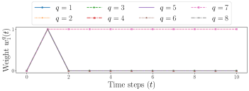
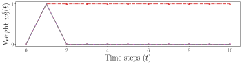
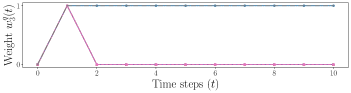
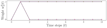
Figure 1: PBRAG  using 8 and large step size $\gamma$. Plots share a common legend.

7 Simulations

In this section, we verify our major claims and illustrate some interesting features of our algorithms.

7-A Fast convergence of PBRAG  with large step-size

Here, we simulate $n=4$ agents to optimally allocate $m=8$ tasks with $r_{i}(q),\phi_{i}(q)\sim\mathrm{Unif}[0,1]$, $\forall i\in\mathcal{A},q\in\mathcal{Q}$. In particular, Table I gives the approximate values of $f_{i}(q)$, $\forall i\in\mathcal{A}$, $q\in\mathcal{Q}$. For each $q\in\mathcal{Q}$, the highlighted cell represents $\max_{i\in\mathcal{A}}f_{i}(q)$.

We first verify the claim in Remark 5.4. Figure 1 shows the solution evolution using 8 from an initial $\mathbf{W}(0)=\mathbf{0}$. Optimal partition as in Figure 1 is given as $\mathcal{V}_{1}=\{2,7\}$, $\mathcal{V}_{2}=\{4\}$, $\mathcal{V}_{3}=\{1,8\}$, $\mathcal{V}_{4}=\{3,5,6\}$. Here, since the values of $f_{i}\in[0,1]$, $\gamma^{q}_{i}\in O(10^{6})$ was required to make the solutions converge in two time steps. For larger deviations in the values of $f_{i}$, much smaller values of $\gamma^{q}_{i}$’s can achieve similar effects.

7-B Effect of constant step-size on d-PBRAG

Here, we deal with the claims in Theorem 6.3 for $n=8$ agents optimally allocating $m=1$ task. We take $f_{1}(1)=B$, $f_{2}(1)=0.9\,B$, and $f_{i}(1)=0.3\,B/i$, $\forall\,i\in\{3,\cdots,8\}$, with $B=1000$. Thus agent $1$ is the dominating agent. Further, we consider an unknown reward structure with $z^{q}_{i}(t)=f_{i}(q)+a^{q}_{i}\,\cos(b^{q}_{i}\,t)\mathrm{exp}(-c^{q}_{i}\,t)$, $\forall i\in\mathcal{A}$, $\forall q\in\mathcal{Q}$, where $a^{q}_{i}\sim\mathrm{Unif}[0,f_{i}(q)]$, $b^{q}_{i}\sim\mathrm{Unif}[0,10]$, and $c^{q}_{i}\sim\mathrm{Unif}[0,1]$. We set the communication graph $\mathcal{G}=(\mathcal{A},\mathcal{E})$ with $\mathcal{E}=\{(1,2),(2,3),(3,4),(4,1)\}$.

Figure 2 shows the solution evolution using 11 with constant step-size from an initial $\mathbf{W}(0)=\mathbf{0}$. It is interesting to note from Figure 2 that if $\varepsilon$ is large, then $w^{1}_{1}(t)$ reaches $1$ faster, but the weights of the non-dominating agents rise higher. On the other hand if $\varepsilon$ is small, then the rise in the weights of the non-dominating agents is less but $w^{1}_{1}(t)$ reaches $1$ slower. This is because $\varepsilon$ affects the choice of $T$ as well.

7-C d-PBRAG  with time-varying step-sizes

Here, we again simulate $n=4$ agents optimally allocating $m=8$ tasks. We take the unknown reward structure as in Section 7-B with $f_{i}(q)$ as in Table I. Further, we use the distributed approach using 11 with time-varying step-sizes as described in Theorem 6.4. We also set the communication graph $\mathcal{G}$ as in Section 7-B.

Figure 3 shows the solution evolution using 11 from an initial $\mathbf{W}(0)=\mathbf{0}$. Optimal partition as in Figure 3 is given as $\mathcal{V}_{1}=\{2,7\}$, $\mathcal{V}_{2}=\{4\}$, $\mathcal{V}_{3}=\{1,8\}$, $\mathcal{V}_{4}=\{3,5,6\}$. This is exactly same as the observation in Section 7-A. Further, notice from Figure 3 that the weights of agents $3$ and $4$ take longer time to settle than agents $1$ and $2$. In general, convergence rate of the algorithm depends on the properties of the unknown reward sequences and hence is difficult to characterize.

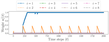
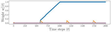
Figure 2: d-PBRAG  for unknown rewards with constant step-size using 11 on cyclic communication graph. Step-size $\gamma^{q}_{i}(t)$ and time-period $T$ were chosen as in Theorem 6.3 with different $\varepsilon$ and $\nu=0.1$. The plots share a common legend. (Top) $\varepsilon=0.9$. (Bottom) $\varepsilon=0.3$.

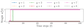
Figure 3: d-PBRAG  for unknown rewards with time-varying step-size using 11 on cyclic communication graph. The plots share a common legend.

8 Conclusion and Future Work

In this paper, we presented a game theoretic formulation of an optimal task allocation problem for a group of agents. By allowing agents to assign weights between zero and one for each task, we relaxed the combinatorial nature of the problem. This led to a partition and weight game, whose NE formed a superset of the optimal task partition. Then, we provided a distributed best-response projected gradient ascent by which convergence to the NE of the weight game was guaranteed.

Future work will consider constraints on number of tasks for each agent, and generalizing the setup to continuous space of tasks and classes of tasks.

References

• [1] H. L. Choi, L. Brunet, and J. P. How, “Consensus-based decentralized auctions for robust task allocation,” IEEE Transactions on Robotics, vol. 25, no. 4, pp. 912–926, 2009.
• [2] F. Bullo, E. Frazzoli, M. Pavone, K. Savla, and S. L. . Smith, “Dynamic vehicle routing for robotic systems,” Proceedings of the IEEE, vol. 99, no. 9, pp. 1482–1504, 2011.
• [3] A. Sadeghi and S. L. Smith, “Heterogeneous task allocation and sequencing via decentralized large neighborhood search,” Unmanned Systems, vol. 5, no. 02, pp. 79–95, 2017.
• [4] H. W. Kuhn, “The Hungarian method for the assignment problem,” Naval Research Logistics, vol. 2, no. 1–2, p. 83–97, May 1955.
• [5] S. Chopra, G. Notarstefano, M. Rice, and M. Egerstedt, “A distributed version of the Hungarian method for multirobot assignment,” IEEE Transactions on Robotics, vol. 33, no. 4, pp. 932–947, 2017.
• [6] J. Cerquides, A. Farinelli, P. Meseguer, and S. D. Sarvapali, “A tutorial on optimization for multi-agent systems,” The Computer Journal, vol. 57, no. 6, pp. 799–824, 2014.
• [7] A. Prasad, S. Sundaram, and H. L. Choi, “Min-max tours for task allocation to heterogeneous agents,” in IEEE Int. Conf. on Decision and Control, 2018, pp. 1706–1711.
• [8] N. Rezazadeh and S. S. Kia, “Distributed strategy selection: A submodular set function maximization approach,” Automatica, vol. 153, p. 111000, 2023.
• [9] J. Vondrák, “Optimal approximation for the submodular welfare problem in the value oracle model,” in ACM Symposium on Theory of Computing, 2008, pp. 67–74.
• [10] G. Calinescu, C. Chekuri, M. Pal, and J. Vondrák, “Maximizing a monotone submodular function subject to a matroid constraint,” SIAM Journal on Computing, vol. 40, no. 6, pp. 1740–1766, 2011.
• [11] S. Lloyd, “Least squares quantization in PCM,” IEEE Transactions on Information Theory, vol. 28, no. 2, p. 129–137, 1982.
• [12] M. Santos, Y. Diaz-Mercado, and M. Egerstedt, “Coverage control for multirobot teams with heterogeneous sensing capabilities,” IEEE Robotics and Automation Letters, vol. 3, no. 2, pp. 919–925, 2018.
• [13] M. Santos and M. Egerstedt, “Coverage control for multi-robot teams with heterogeneous sensing capabilities using limited communications,” in IEEE/RSJ Int. Conf. on Intelligent Robots & Systems, 2018, pp. 5313–5319.
• [14] J. Cortés, S. Martinez, T. Karatas, and F. Bullo, “Coverage control for mobile sensing networks,” IEEE Transactions on Robotics and Automation, vol. 20, no. 2, pp. 243–255, 2004.
• [15] E. Frazzoli and F. Bullo, “Decentralized algorithms for vehicle routing in a stochastic time-varying environment,” in IEEE Int. Conf. on Decision and Control, Paradise Island, Bahamas, Dec. 2004, pp. 3357–3363.
• [16] M. Zhu and S. Martínez, “Distributed coverage games for energy-aware mobile sensor networks,” SIAM Journal on Control and Optimization, vol. 51, no. 1, pp. 1–27, 2013.
• [17] J. R. Marden, G. Arslan, and J. S. Shamma, “Cooperative control and potential games,” IEEE Transactions on Systems, Man, & Cybernetics. Part B: Cybernetics, vol. 39, no. 6, p. 1393–1407, 2009.
• [18] R. Konda, R. Chandan, D. Grimsman, and J. R. Marden, “Balancing asymptotic and transient efficiency guarantees in set covering games,” in American Control Conference, 2022, pp. 4416–4421.
• [19] P. Frihauf, M. Krstic, and T. Basar, “Nash equilibrium seeking for games with non-quadratic payoffs,” in IEEE Int. Conf. on Decision and Control, Atlanta, USA, December 2010, pp. 881–886.
• [20] M. Ye and G. Hu, “Distributed Nash equilibrium seeking by a consensus based approach,” IEEE Transactions on Automatic Control, vol. 62, no. 9, pp. 4811–4818, 2017.
• [21] Z. Deng and X. Nian, “Distributed generalized Nash equilibrium seeking algorithm design for aggregative games over weight-balanced digraphs,” IEEE Transactions on Neural Networks and Learning Systems, vol. 30, no. 3, pp. 695–706, 2018.
• [22] J. Koshal, A. Nedić, and U. V. Shanbhag, “A gossip algorithm for aggregative games on graphs,” in IEEE Int. Conf. on Decision and Control, 2012, pp. 4840–4845.
• [23] F. Salehisadaghiani and L. Pavel, “Distributed Nash equilibrium seeking: A gossip-based algorithm,” Automatica, vol. 72, pp. 209–216, 2016.
• [24] A. C. Chapman, R. A. Micillo, R. Kota, and N. R. Jennings, “Decentralized dynamic task allocation using overlapping potential games,” The Computer Journal, vol. 53, no. 9, pp. 1462–1477, 2010.
• [25] Y. Narahari, Game theory and mechanism design.   World Scientific, 2014, vol. 4.
• [26] R. Diestel, “Graph theory,” Graduate Texts in Mathematics, pp. 173–207, 2017.