Microscopic aspects of $\gamma$ softness in atomic nuclei

Abstract

It is demonstrated that the Triaxial Projected Shell Model reproduces the energies and transition probabilities of the nucleus ¹⁰⁴Ru and the rigid triaxial nucleus ¹¹²Ru. An interpretation in terms of band mixing is provided.

My presentation covers published work Jehangir ; Ruoofa , a paper under review Ruoofb and ongoing work Ruoofc . I start with discussing the concept of $\gamma$ softness vs. $\gamma$ rigidness and the corresponding observables in the traditional frame work of a phenomenological Bohr Hamiltonian. Then I sketch the Triaxial Projected Shell Model (TPSM) and compare calculations for ^104,122Ru with experiment. Finally I discuss the TPSM interpretation of the appearance $\gamma$ softness or $\gamma$ rigidness, which is an anternative perspective traditional concept of a collective Hamiltonian.

The notation of $\gamma$ softness came into use in the context of the Bohr Hamiltonian (BH) which describes collective states of the quadrupole distortion of the nuclear surface BMII , where the parameter $\beta$ describes the deformation and $\gamma$ the triaxiality. The simple Gamma Rotor Hamiltonian of Ref. caprio11 is one possibility to quantify the concept of $\gamma$ softness. The deformation $\beta$ is assumed to be fixed. The scaled BH in the $\gamma$ degree of freedom

$$\hat{\Lambda}^{2}+V(\gamma)=\hat{\Lambda}^{2}-\chi\cos 3\gamma+\xi\cos^{2}3\gamma$$ (1)

contains a potential determined by the parameters $\chi$ and $\xi$ and a kinetic term

$$\hat{\Lambda}^{2}=-\biggl{(}\frac{1}{\sin 3\gamma}\frac{\partial}{\partial\gamma}\sin 3\gamma\frac{\partial}{\partial\gamma}-\frac{1}{4}\sum_{i=1,2,3}\frac{\hat{L}_{i}^{\prime 2}}{\sin^{2}(\gamma-\frac{2}{3}\pi i)}\biggr{)},$$ (2)

which is the sum of the $\gamma$ kinetic energy and the rotational energy.

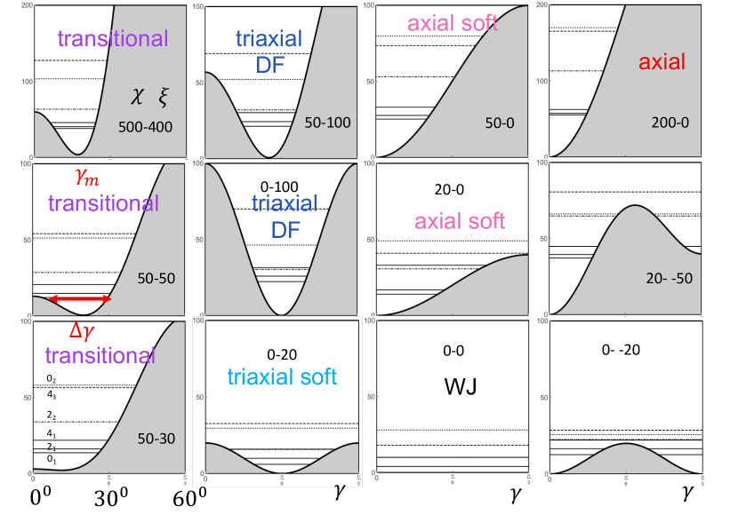
Figure 1: Selection of potentials given by Eqn. (1). The potential parameters are included as $\chi-\xi$. The energies of the lowest states are shown as horizontal lines, where the line type indicates the $I_{n}$ of the state (see the panel 50-30). The potential minimum at $\gamma_{m}$ is a measure of the triaxiality and the width $\Delta\gamma$ is a measure how soft the potential is. To simplify terminology, "axial" or "triaxial" denote the cases with a small width. DF stands for the approach to rigid triaxial rotor (Dawydov-Fillipov limit) and W J for the $\gamma$ independent case (Wilet-Jean). Modified from Ref. Ruoofb .

Table 1: Triaxiality characteristics of the potentials plotted in Fig. 1 . The staggering parameter $\bar{S}(I)$ is defined by Eq. (4). The excitation energy $E(2^{+}_{1})_{GR}$ is the difference $E(2^{+}_{1})-E(0^{+}_{1})$ of the eigenvalues of the Gamma Rotor Hamiltonian (1).

$\chi-\kappa$	$E(2^{+}_{1})_{GR}$	$\gamma_{m}$	$\Delta\gamma$	${\frac{E(2^{+}_{2})}{E(2^{+}_{1})}}$	${\frac{E(2^{+}_{2})}{E(4^{+}_{1})}}$	$\bar{S}(6)$	$Q(2^{+}_{1})$	$\begin{array}[]{l}B(E2,2^{+}_{2}\\ \rightarrow 0^{+}_{1})\end{array}$
100-0	2.24	0	17	18.0	3.31	-0.14	-0.878	0.047
50-0	2.39	0	20	11.6	3.55	-0.51	-0.861	0.064
20-0	2.87	0	24	5.82	1.93	-1.75	-0.797	0.079
0-0	4.00	30	60	2.50	1.00	-2.75	0.000	0.000
0-200	3.05	30	16	2.11	0.81	3.87	0.000	0.000
0-100	3.57	30	19	2.21	0.86	3.12	0.000	0.000
0-20	3.95	30	22	2.45	0.98	0.50	0.000	0.000
50-100	3.10	25	19	3.50	1.20	1.85	-0.693	0.084
500-400	2.34	17	15	10.8	3.17	0.32	-0.861	0.066
50-30	2.58	11	26	7.78	2.44	-0.35	-0.835	0.082
0- -20	3.39	30	35	2.42	0.96	-5.79	0.000	0.000
20- -50	2.35	34	17	11.74	3.62	-5.55	-0.868	0.032

Fig. 1 shows examples of various potentials, which illustrate the notations of rigid vs. soft and triaxial vs. axial. Tab. 1 lists the main characteristics of the collective mode. The position of the minimum (maximum) of the potentials $\gamma_{m}$ quantifies the degree of triaxiality. The softness of the potentials $\Delta\gamma$ is quantified as the length of the bar E($0^{+}_{1})<V(\gamma)$, which is a measure of the ground-state fluctuation in $\gamma$. The next twocolumns list important energy criteria, which characterize the nature of triaxiality, namely the ratios ${\left[\frac{E(2^{+}_{2})}{E(2^{+}_{1})}\right]}$, ${\left[\frac{E(2^{+}_{2})}{E(4^{+}_{1})}\right]}$.

The staggering parameter $S(I)$ of the $\gamma$ band is an essential observable indicating the $\gamma$ softness NV91 .

$$S(I)=[E(I)-2E(I-1)]+E(I-2)]/E(2^{+}_{1}),$$ (3)

$$\bar{S}(I)=[S(I)-S(I+1)]/2.$$ (4)

The odd-$I$-down pattern indicates the concentration of the collective wave function around a finite $\gamma$-value (static triaxiality), whereas the even-I-down pattern points to a spread of the wave function over a large range of $\gamma$ (dynamic triaxiality). Tab. 1 lists the modified staggering parameter $\bar{S}(6)$.

Fig. 2 shows the experimental signatures of triaxiality in ^104,112Ru. Added are the two potentials from Fig. 1, which according to Tab. 1 provide the best description of the energetic characteristics. Clearly, ¹⁰⁴Ru is a very $\gamma$ soft nucleus while the triaxial shape is well established in ¹¹²Ru.

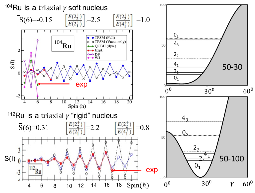
Figure 2: Phenomenlogical potentials (see Fig. 1) which best reproduce the shown experimental signatures of triaxiality in ^104,112Ru (see Tab. 1). Combination from Refs. Jehangir ; Ruoofa ; Ruoofb ; Ruoofc .

The details of the TPSM are described in Refs. Jehangir ; Ruoofa ; Ruoofb ; Ruoofc . The basic methodology of the TPSM approach is similar to that of the standard spherical shell model with the exception that angular-momentum projected deformed basis is employed to diagonalize the shell model Hamiltonian. The Hamiltonian consists of monopole pairing, quadrupole pairing, and quadrupole-quadrupole interaction terms within the configuration space of three major oscillator shells ($N=3,4,5$ for neutrons and $N=2,3,4$ for protons)

$$\hat{H}=\hat{H}_{0}-{1\over 2}\chi\sum_{\mu}\hat{Q}^{\dagger}_{\mu}\hat{Q}_{\mu}-G_{M}\hat{P}^{\dagger}\hat{P}-G_{Q}\sum_{\mu}\hat{P}^{\dagger}_{\mu}\hat{P}_{\mu},$$ (5)

where $\hat{H}_{0}$ is the spherical single-particle potential BMII . The pairing constant $G_{M}$ is determined by the BSC relation $G_{M}\,<\!\hat{P}\!>\,=\Delta$. The quadrupole pairing strength $G_{Q}$ is assumed to be 0.18 times $G_{M}$. The QQ-force strength $\chi$ is obtained by the self-consistency relation $2\hbar\omega\varepsilon=3\chi\,<\!\Phi\,|\,\hat{Q}_{0}\,|\,\Phi\!>\,$. The shell model Hamiltonian (5) is diagonalized in the space of angular-momentum projected multi-quasiparticle configurations generated by the triaxial version of the Nilsson Hamiltonian BMII with the deformation parameters $\varepsilon$ and $\gamma$. The basis is composed of the 0-qp vacuum, the two-quasiproton, the two-quasineutron and the combined four-quasiparticle configurations

$$\hat{P}^{I}_{MK}\,|\,\Phi\!>\,,\leavevmode\nobreak\ \hat{P}^{I}_{MK}\leavevmode\nobreak\ a^{\dagger}_{p_{1}}a^{\dagger}_{p_{2}}\,|\,\Phi\!>\,,\leavevmode\nobreak\ \hat{P}^{I}_{MK}\leavevmode\nobreak\ a^{\dagger}_{n_{1}}a^{\dagger}_{n_{2}}\,|\,\Phi\!>\,,$$

$$\hat{P}^{I}_{MK}\leavevmode\nobreak\ a^{\dagger}_{p_{1}}a^{\dagger}_{p_{2}}a^{\dagger}_{n_{1}}a^{\dagger}_{n_{2}}\,|\,\Phi\!>\,,$$ (6)

The TPSM has $\Delta_{p,n},\leavevmode\nobreak\ \varepsilon$ and $\gamma$ as input parameters. The pairing gaps $\Delta_{p,n}$ are chosen such that the overall observed odd-even mass differences are reproduced for nuclei in the considered region. The deformation parameter $\varepsilon$ is taken from $B(E2,2_{1}^{+}\rightarrow 0_{1}^{+})$ systematics or mean field equilibrium deformations. The triaxiality parameter $\gamma$ is adjusted to reproduce the $\gamma$ band head energy $E(2^{+}_{2})$.

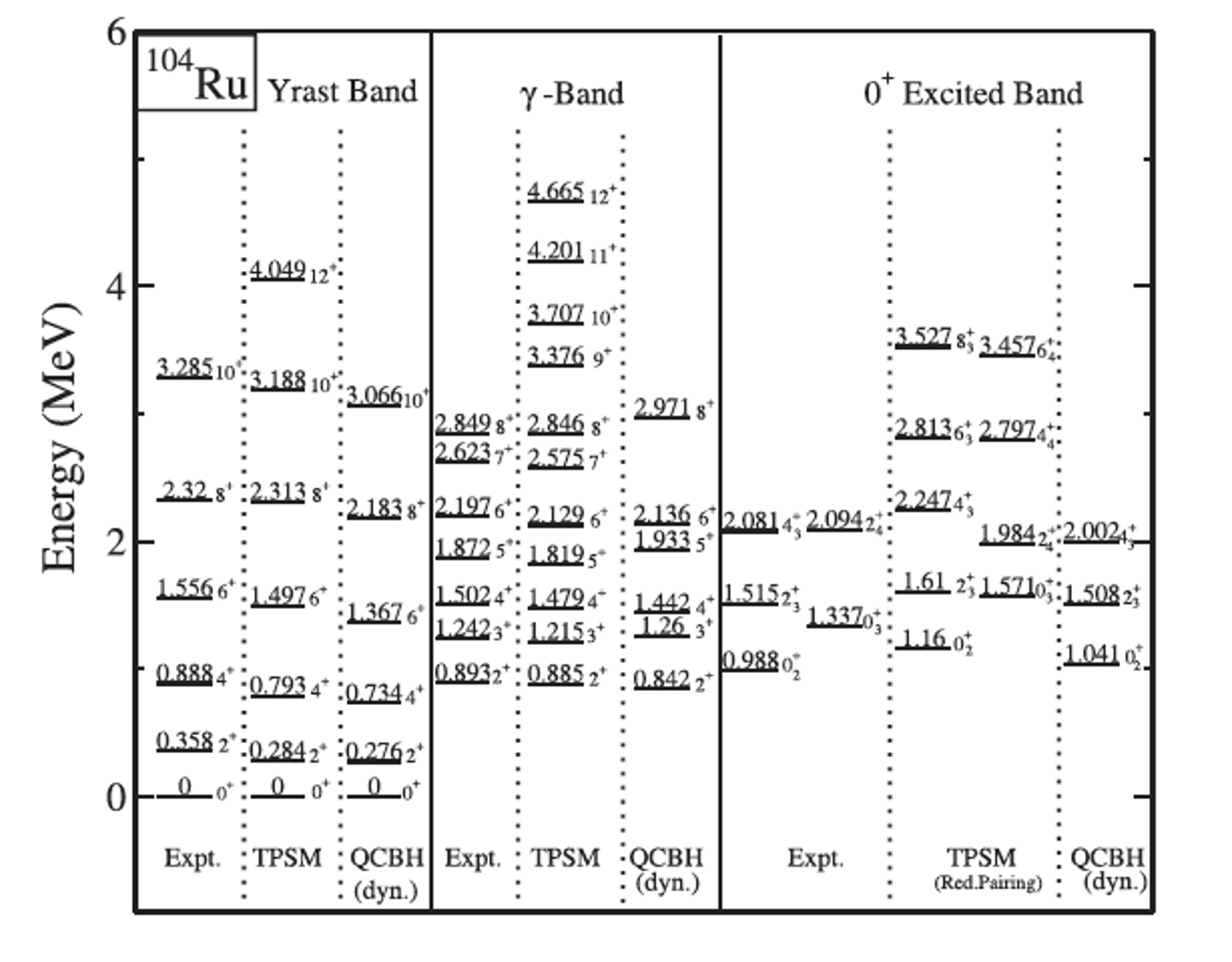
Figure 3: Comparison of the experimental levels of ¹⁰⁴Ru with the calculations by means of the TPSM and the microscopic Bohr Hamiltonian Ru104 (QCBH dyn). From Ref. Ruoofa .

Fig. 3 demonstrates that the TPSM very well reproduces the experimental energies of the ground, $\gamma$ and excited $0^{+}$ bands. In particular, the even-I-down pattern of the staggering parameter $S(I)$ of the $\gamma$ band is quantitatively reproduced, which is the energy signature $\gamma$ softness (see Fig. 2). Tables 2, 3 compare the TPSM with the large number of reduced $E2$ and $M$ matrix element measured in the COULEX experiment of Ref. Ru104 . The agreement of the TPSM results with the COULEX data is remarkable, because the $E2$ matrix elements provide the most direct information on the statics and dynamics of the collective quadrupole modes. Comparing the "Full" matrix elements with "Vacu." ones shows that the quasiparticle admixtures generate substantial shifts that generate the good agreement with the experiment.

Figs. 4 and 5 depict the quadrupole shape invariants DC86 and their dispersions calculated from the reduced $E2$ matrix elements. The invariant $\,<\!I^{+}_{n}|Q^{2}|I^{+}_{n}\!>\,$ measures the average intrinsic deformation of a state $I^{+}_{n}$. The invariant $\,<\!I^{+}_{n}|\cos 3\delta|I^{+}_{n}\!>\,$ contains the information about the triaxiality of the intrinsic shape, where $\delta=\arctan{\,<\!I^{+}_{n}|\cos 3\delta|I^{+}_{n}\!>\,}$. The invariant $Q$ is approximately proportional to $\beta$, and the invariant $\delta$ is approximately equal to $\gamma$ of the liquid drop model BMII .

The ground-band TPSM values of $\,<\!\cos 3\delta\!>\,\sim 0.5$ in Fig. 4 signify a substantial triaxiality with preference for prolate shape, corresponding to $\gamma\approx 20^{\circ}$. The TPSM dispersion $\sigma<\cos 3\delta>\sim 0.3$ indicates large fluctuations of the triaxiality parameter with 70% of the distribution within the range $9^{\circ}<\gamma<24^{\circ}$. Hence, the TSPM shape invariants imply that ¹⁰⁴Ru is $\gamma$ soft, which is in accordance with the experimental staggering parameter $S(I)$ and $\bar{S}(6)=-0.15$ in Fig. 2.

The shape invariants for ¹¹²Ru in Fig. 5 correspond to narrow distributions of $7^{\circ}$ width centered at $\gamma\approx 26^{\circ}$ for the ground band and $\gamma\approx 20^{\circ}$ for the $\gamma$ band. They indicate a well established triaxial shape, which is consistent with the experimental even -I- up pattern of $S(I)$ and $\bar{S}(6)=0.31$ in Fig. 2.

Table 2: Comparison of all known experimental reduced $E2$ diagonal, in-band and inter-band matrix elements $\,<\!I_{i}||E2||I_{f}\!>\,(e.b)$, (associated errors in parenthesis) and calculated ones for yrast- and $\gamma$-band of ¹⁰⁴Ru. From Ref. Ruoofa .

$I_{i}\rightarrow I_{f}$	Expt.	TPSM	TPSM	$I_{i}\rightarrow I_{f}$	Expt.	TPSM	TPSM
		(Full)	(Vacu.)			(Full)	(Vacu.)
$2_{1}\rightarrow 2_{1}$	-0.71(11)	-0.817	-0.634	$4_{2}\rightarrow 3_{1}$	$\pm$0.68 (5)	-0.787	-0.597
$4_{1}\rightarrow 4_{1}$	-0.79(15)	-0.906	-0.437	$5_{1}\rightarrow 3_{1}$	1.22(4)	1.184	0.697
$6_{1}\rightarrow 6_{1}$	-0.70(${}^{+30}_{-20}$ )	-0.868	-0.342	$6_{2}\rightarrow 4_{2}$	1.52 (12)	1.521	0.682
$8_{1}\rightarrow 8_{1}$	-0.6(${}^{+3}_{-5}$ )	-0.855	-0.297	$8_{2}\rightarrow 6_{2}$	2.02(4)	2.056	0.747
$2_{2}\rightarrow 2_{2}$	0.62(8)	0.648	0.633	$2_{2}\rightarrow 0_{1}$	-0.156 (2)	-0.141	-0.225
$4_{2}\rightarrow 4_{2}$	-0.58(18)	-0.749	-0.534	$2_{2}\rightarrow 2_{1}$	-0.75(4)	-0.722	-0.612
$6_{2}\rightarrow 6_{2}$	$\pm$1.0(3)	-1.105	-0.763	$2_{2}\rightarrow 4_{1}$	$\epsilon$ [-0.1, 0.1]	-0.090	-0.001
$2_{1}\rightarrow 0_{1}$	0.917 (25)	0.973	0.901	$3_{1}\rightarrow 2_{1}$	0.22(10)	0.254	0.302
$4_{1}\rightarrow 2_{1}$	1.43 (4)	1.591	1.456	$3_{1}\rightarrow 4_{1}$	-0.57	-0.517	-0.559
$6_{1}\rightarrow 4_{1}$	2.04 (8)	2.081	1.830	$4_{2}\rightarrow 2_{1}$	-0.107 (8 )	-0.113	-0.054
$8_{1}\rightarrow 6_{1}$	2.59 (${}^{+24}_{-9}$ )	2.486	1.902	$4_{2}\rightarrow 4_{1}$	-0.83(5)	-0.840	-0.505
$10_{1}\rightarrow 8_{1}$	2.7 (6)	2.668	1.623	$6_{2}\rightarrow 4_{1}$	-0.22(${}^{+6}_{-12}$ )	-0.230	-0.682
$3_{1}\rightarrow 2_{2}$	-1.22 (10)	-1.241	-0.935	$6_{2}\rightarrow 6_{1}$	$>$-0.84	-0.947	-0.411
$4_{2}\rightarrow 2_{2}$	1.12(5)	1.095	0.510

Table 3: Comparison of all known experimental reduced $E2$ matrix elements $\,<\!I_{i}||E2||I_{f}\!>\,(e.b)$, diagonal, in-band and inter-band values (associated errors in parenthesis) and calculated ones for excited $0^{+}$ bands of ¹⁰⁴Ru. From Ref. Ruoofa .

$I_{i}\rightarrow I_{f}$	Expt.	TPSM	$I_{i}\rightarrow I_{f}$	Expt.	TPSM
$2_{3}\rightarrow 0_{2}$	0.71(4)	0.682	$2_{3}\rightarrow 4_{1}$	-0.370(4)	-0.311
$4_{3}\rightarrow 2_{3}$	0.75(25)	0.613	$2_{3}\rightarrow 2_{2}$	$\pm$0.22(${}^{+25}_{-5}$)	-0.237
$0_{2}\rightarrow 2_{1}$	-0.266(8)	-0.221	$2_{3}\rightarrow 4_{2}$	0.31(${}^{+13}_{-6}$)	0.221
$0_{2}\rightarrow 2_{2}$	0.08 (3)	0.099	$2_{3}\rightarrow 4_{4}$	0.53(${}^{+32}_{-14}$)	0.481
$2_{3}\rightarrow 0_{1}$	-0.071(3)	-0.048	$0_{3}\rightarrow 2_{1}$	$>$-0.1	-0.201
$2_{3}\rightarrow 2_{1}$	$\pm$0.07(3)	-0.031	$2_{3}\rightarrow 2_{3}$	-0.08(${}^{11}_{25}$)	-0.631

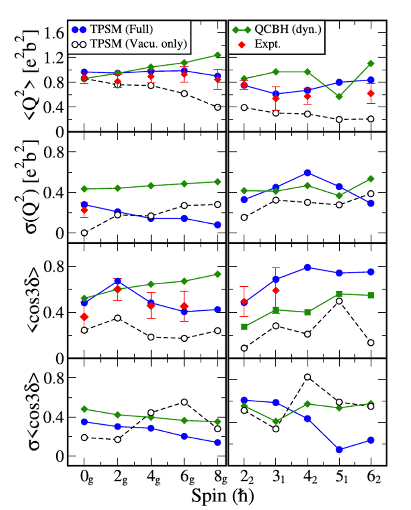
Figure 4: Comparison of the observed (Expt.) with the TPSM shape invariants for the ground-band (left panels) and $\gamma$-band (right panels) in ¹⁰⁴Ru. The results from the microscopic Bohr Hamiltonian Ru104 (QCBH dyn) are included. From Ref. Ruoofa .

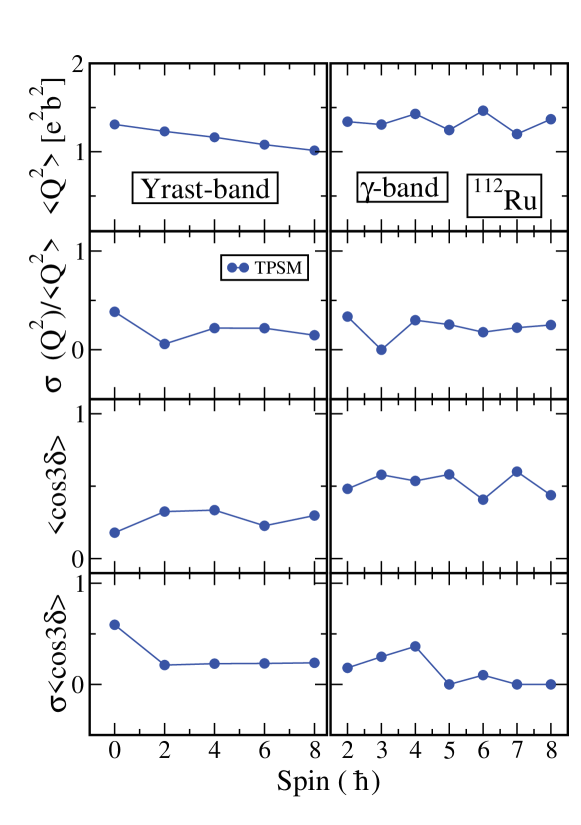
Figure 5: As Fig. 4 for ¹¹²Ru. From Ref.Ruoofc .

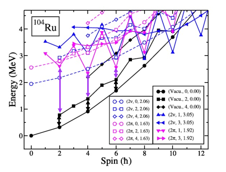
Figure 6: TPSM projected energies before band mixing. The bands are labelled by three quantities : quasiparticle character, $K$-quantum number and energy of the two-quasiparticle state. For instance, $(2\pi,\leavevmode\nobreak\ 1,\leavevmode\nobreak\ 1.92)$ designates the $K=1$ state projected from the $h_{11/2}$ two-quasiproton configuration with the energy of 1.92 MeV. The $K=0,\leavevmode\nobreak\ 2,\leavevmode\nobreak\ 4$ states projected from the quasiparticle vacuum are labelled with Vacu. The four-quasiparticle states lie above 5 MeV. The black arrows indicate the repulsion by the coupling to the ground band and the purple arrows the repulsion by coupling to the even states of the $(2\pi,\leavevmode\nobreak\ 1,\leavevmode\nobreak\ 1.92)$ band after band mixing. Modified from Ref. Ruoofa .

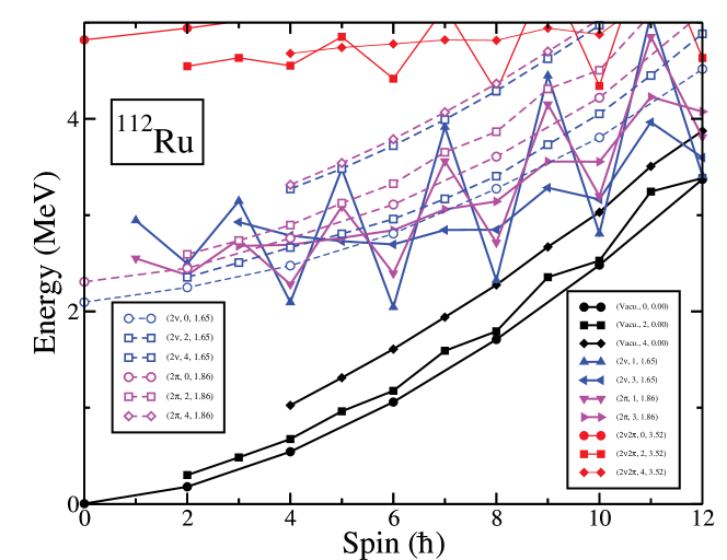
Figure 7: As Fig. 6 for ¹¹²Ru. From Ref. Ruoofc .

The TPSM provides an alternative perspective on the experimental signatures of $\gamma$ softness. The staggering parameter of the $\gamma$ band is an important signature. Fig. 6 displays the energies of the projected quasiparticle configurations in ¹⁰⁴Ru. Diagonalizing the Hamitonian within this basis generates repulsions between neighboring states.

The $K=2$ vacuum sequence, associated with the $\gamma$ band, shows the even-I-down pattern. Mixing it with the $K=0$ vacuum states, associated with the ground band, pushes the even -I states of the $K=2$ band up. There is no shift for odd I, because the ground band contains only even-I states (see black arrows in Fig. 6). The triaxial rotor even-I-up pattern emerges for sufficiently strong interaction. This is the TPSM result when the basis is truncated to the $K$ states projected from zero quasiparticle state, which is shown as "Vacu. only" (black dashed) in Fig. 2. The same even-I-up are results found for "Vacu. only" for all 35 studied nuclei Jehangir ; Ruoofa .

Admixing the lowest projected two quasiparticle states $(2\pi,\leavevmode\nobreak\ 1,\leavevmode\nobreak\ 1.92)$ (see purple arrows in Fig. 6) and $(2\nu,\leavevmode\nobreak\ 1,\leavevmode\nobreak\ 3.05)$ pushes the even-I states of the $K=2$ vacuum sequence down. There is less repulsion for odd I because of the larger distance. This repulsion prevails over the one by the ground band, and the triaxial rotor pattern changes to the $\gamma$ soft pattern even-I-down. The pattern flip is seen in Fig. 2 as the opposite staggering phases of the "Full" results (blue dashed) compared to the "Vacu. only" (black dashed) ones.

Fig. 7 displays the energies of the projected quasiparticle configurations in ¹¹²Ru. The distance between the $K=2$ and $K=0$ sequences projected from the vacuum is much smaller than for ¹⁰⁴Ru. Their mixing is stronger and the corresponding shift is larger. It prevails over the downshift by the repulsion of the two-qusiparticle sequences, such the staggering amplitude is reduced but its phase remains unchanged (see Fig. 2).

The competition between the two kinds of band mixing accounts for the observed $S(I)$ pattern for the 35 nuclides studied in Refs. Jehangir ; Ruoofa ; Ruoofb ; Ruoofc . The mixing with the two-quasiparticle states provides a natural explanation for the observed rapid change of the $S(I)$ with $N$ and $Z$, because the quasiparticle structure near the Fermi level plays a central role. The mixing interpretation explains also the $Z-N$ dependence of the triaxiality characteristics of transition probabilities Ruoofb .

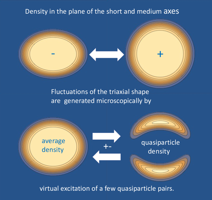
Figure 8: Summary: One of the main research themes in quantum many-body systems is the emergence of collective features from microscopic degrees of freedom. Using the microscopic approach of the triaxial projected shell model, the authors demonstrate that admixing a few quasiparticle excitations into the vacuum configuration with a fixed triaxiality parameter $\gamma$ provides a quantitative description of the shape fluctuations of the $\gamma$-soft nucleus ¹⁰⁴Ru. The collective features are elucidated using the quadrupole shape invariant analysis, and also the staggering phase classification of the $\gamma$ band. Figure and text from the editor’s suggestion in Phys. Rev. C 107, Issue 2, (2023).

References

- (1) S. Jehangir, G.H. Bhat, J.A. Sheikh, S. Frauendorf, W. Li, R. Palit, N.Rather, Eur. Phys. J. A 57, 308 (2021).
- (2) S.P. Rouoof, Nazira Nazir, S. Jehangir, G.H. Bhat, J.A. Sheikh, N. Rather, S. Frauendorf, Phys. Rev. C 107, L021303 (2023).
- (3) S.P. Rouoof, Nazira Nazir, S. Jehangir, G.H. Bhat, J.A. Sheikh, N. Rather, S. Frauendorf, Eur. Phys. J. A, in revision, arXiv:2307.06670.
- (4) S.P. Rouoof, S. Jehangir, Nazira Nazir, G.H. Bhat, J.A. Sheikh, N. Rather, S. Frauendorf, Eur. Phys. J. A, in preparation.
- (5) A. Bohr and B. R. Mottelson, Nuclear Structure, Vol. II (Benjamin Inc., New York, 1975).
- (6) M. A. Caprio, Phys. Rev. C 83, 064309 (2011).
- (7) N. V. Zamfir and R. F. Casten, Phys. Lett. B 3, 260 (1991).
- (8) K. Zajac, L. Próchniak, K. Pomorski, S.G. Rohoziński and J. Srebrny, Nucl. Phys. A 653, 71 (1999).
- (9) D. Cline, Ann. Rev. of Nucl. and Part. Science, 36, 683 (1986).