Best of Both Worlds: Stochastic and Adversarial
Convex Function Chasing

Abstract

Convex function chasing (CFC) is an online optimization problem in which during each round $t$, a player plays an action $x_{t}$ in response to a hitting cost $f_{t}(x_{t})$ and an additional cost of $c(x_{t},x_{t-1})$ for switching actions. We study the CFC problem in stochastic and adversarial environments, giving algorithms that achieve performance guarantees simultaneously in both settings. Specifically, we consider the squared $\ell_{2}$-norm switching costs and a broad class of quadratic hitting costs for which the sequence of minimizers either forms a martingale or is chosen adversarially. This is the first work that studies the CFC problem using a stochastic framework. We provide a characterization of the optimal stochastic online algorithm and, drawing a comparison between the stochastic and adversarial scenarios, we demonstrate that the adversarial-optimal algorithm exhibits suboptimal performance in the stochastic context. Motivated by this, we provide a best-of-both-worlds algorithm that obtains robust adversarial performance while simultaneously achieving near-optimal stochastic performance.

Keywords — online learning algorithms, dynamic programming, smoothed online optimization, competitive analysis, regret analysis, stochastic-adversarial trade-off

1 Introduction

Convex Function Chasing (CFC) represents a class of problems in which a player encounters a convex hitting cost $f_{t}(x)$ during each round $t$ and must make an online decision $x_{t}$ from an action space in $\mathbb{R}^{d}$. Along with the hitting cost, selecting an action incurs a switching cost $c(x_{t},x_{t-1})$. In this paper, we focus on a popular class of quadratic hitting cost functions $f_{t}(x)=\frac{1}{2}(x-v_{t})^{T}A(x-v_{t})$ and squared $\ell_{2}$-norm switching cost, i.e., $c(x_{t},x_{t-1})=\frac{1}{2}\|x_{t}-x_{t-1}\|_{2}^{2}$. CFC was introduced by [13] as a continuous-space extension of several essential online learning problems, such as the $k$ server problem [21] and Metrical Task Systems (MTS) [7]. During the last decade, CFC has been explored in various forms, with Smooth Online Convex Optimization (SOCO) [24, 5, 11, 16] being one of the most popular variants. In the SOCO framework, the switching cost $c(x_{t},x_{t-1})$ is expressed as a function of the norm of the action space. The presence of this switching cost makes the problem intricate, as the player must strike a delicate balance between the current hitting cost and the current and future switching costs. Over the past decade, CFC, notably in the form of SOCO, has emerged as a powerful tool with numerous real-world applications. SOCO has been deployed in various fields, including data center management [25, 24, 28, 37], electrical vehicle charging [20, 19, 14], video transmission [18], power systems [30, 27, 4], and chip thermal management [38, 39]. In addition to these, SOCO has recently been applied in control systems [17, 15, 23]. The versatility of CFC in optimizing complex systems across these diverse domains highlights its practical importance and motivates further study.

Since its introduction, the CFC problem has been studied primarily from an adversarial point of view [2, 5, 9, 10, 11, 16, 40, 41]. Consequently, the resulting algorithms tend to be overly pessimistic for situations that may have more structure and potentially stochastic behavior. In related domains, such as scheduling, stochastic modeling has been used to capture known data patterns, and algorithms can then be designed to perform well for these known models. In contrast, adversarially designed algorithms must safeguard against arbitrary inputs and thus cannot exploit the inherent structures within the environment. This trade-off between average-case and worst-case performance is long-standing in the algorithms literature [35, 29, 22, 31]. However, in the case of CFC, the design of algorithms for the case of stochastic hitting cost functions is unexplored. This motivates the following open question, which we study in this paper:

“Is there a simple characterization of a (near-)optimal policy for stochastic CFC? How does the (near-)optimal policy for the stochastic setting compare to policies designed in the adversarial setting?"

Because optimal algorithms for stochastic settings are designed to exploit known model structures, rather than hedge against the potential of an adversarial environment, it is often the case that they can be highly sensitive to the underlying stochastic assumptions. As a result, such algorithms may lack robustness against adversarial input. This represents the other side of the long-standing trade-off between optimizing average-case and worst-case performance, and motivates a foundational question for CFC:

“Is there an algorithm for CFC that achieves near-optimal performance simultaneously in stochastic and adversarial settings?"

Such best-of-both-worlds algorithms are akin to the seminal work by Bubeck and Slivkins [8], which answers the question affirmatively in the multi-arm bandit setting. Best-of-both-worlds algorithms are highly sought after in the algorithms literature; however, they are also rare, and there are key characteristics distinguishing the CFC framework from the multi-arm bandits’ framework of [8], e.g., the infinite action space and the dynamic optimal performance benchmark (as opposed to a focus on static regret), that make it questionable whether such a best-of-both-worlds algorithm exists for CFC.

Contributions. This paper provides answers to both of the questions highlighted above. Specifically, the contributions of this paper are fourfold:

(a) Characterization of a stochastic online optimal algorithm: We start by considering the CFC problem in the setting when the sequence of minimizers $\{v_{t}\}_{t}$ of the hitting cost functions $\{f_{t}\}_{t}$ forms a martingale. In this setting, we design and analyze an online algorithm, referred to as the Lazy Adaptive Interpolation algorithm (lai, Algorithm 1), that is provably optimal in the class of all online algorithms (see Theorem 3.1). We further characterize its expected cost and show that it is $\mathcal{O}(T)$, where $T$ is the time horizon (see Theorem 3.2). Notably, this algorithm is dynamic in nature and, as expected, has a much better performance than any static hindsight-optimal decision (see Theorem 3.4), which achieves a cost that is $\Theta\left(T^{2}\right)$.

(b) Stochastic suboptimality of the adversarial optimal: When adversarial inputs are considered, the performance is measured in terms of the competitive ratio, the worst-case ratio of the cost of an algorithm to the cost of the hindsight optimal sequence of decisions. In [16], the authors propose the robd algorithm and show that it has an optimal competitive ratio among all online algorithms. When the inputs are stochastic, however, we show that the robd algorithm admits a linear regret (in the time horizon $T$) with respect to the stochastic optimal cost, i.e., the cost of the aforementioned lai algorithm (see Theorem 3.6). We achieve this by first identifying that the robd algorithm, in our setup, belongs to the class of what we call Fixed Interpolation algorithms and then showing that in fact, most algorithms in this class admit linear regret (see Theorem 3.8).

(c) Adversarial analysis of stochastic optimal: To understand the robustness of the lai algorithm against adversarial input, we perform its competitive analysis and find it potentially suboptimal (see Theorem 3.9). En route, we also establish competitive ratio bounds for a much wider class of memoryless algorithms, which might be of independent interest. The novelty of our analysis framework lies in its applicability to algorithms with decision rules that change over time (see Theorem 3.11).

(d) Best-of-both-worlds algorithm design: Our final contribution focuses on the design of a best-of-both-worlds algorithm for CFC. We present a novel hyperparametric algorithm called lai$(\gamma)$ (Algorithm 2) with $\gamma\in[0,1]$, which delivers near-optimal performance (see Corollary 3.14) in both stochastic and adversarial environments without leveraging prior knowledge about the nature of the environment. Specifically, the hyperparameter $\gamma\in[0,1]$ determines the algorithm’s position in the trade-off between adversarial and stochastic settings. For any choice of $\gamma\in[0,1]$, the algorithm guarantees (i) a finite regret (that depends on $\gamma$) with respect to the online-optimal lai algorithm, and (ii) a finite competitive ratio (that depends on $\gamma$) with respect to the adversarial-optimal robd algorithm (see Theorem 3.12).

To obtain the results described above, we make a number of contributions on the methodological front. In particular, at the core of our analysis, we characterize the online optimal algorithm in the stochastic setting by leveraging the dynamic programming (DP) machinery. Although the DP framework offers a powerful set of tools for any online decision-making problem, a fundamental difficulty lies in understanding the structure of the value function. In our work, we inductively identify structure in the DP that enables us to express it as a simple, adaptive interpolation algorithm. Beyond our stochastic analysis, in the adversarial setting, the non-stationary nature of our algorithms necessitated an extension of the existing adversarial analysis methods to encompass a broader range of algorithms. Finally, the design of lai$(\gamma)$ draws inspiration from the stochastic optimality conditions of lai and the suboptimal aspects of this algorithm in adversarial scenarios.

We also would like to highlight the ease of implementation of the algorithms proposed in this paper. First, the algorithms do not make any assumptions about the underlying data distribution, allowing them to adapt to changing distribution patterns without compromising performance. Furthermore, the proposed algorithms are memoryless and computationally simple. In contrast to many adversarial algorithms in the existing literature [9, 10, 11, 26], which necessitate solving optimization sub-problems in each iteration, the algorithms in this work do not include such complex subroutines. In fact, there are fundamental limitations to what can be achieved using memoryless algorithms in adversarial scenarios [32], and our results highlight that memoryless algorithms can be optimal in the stochastic setting.

Related work. The body of research on Convex Function Chasing (CFC) is predominantly centered around adversarial results and can be broadly divided into two distinct communities. The first community examines CFC through the lens of Metrical Task Systems and employs the competitive ratio as the performance metric. This ratio measures the algorithm’s total cost in comparison to that of the hindsight optimal decision sequence. Meanwhile, the second community approaches CFC from an Online Convex Optimization (OCO) standpoint and assesses performance by considering one or more forms of regret as the evaluation metric.

SOCO, a popular variant of CFC, was introduced as a means to efficiently manage server uptime in data centers and was initially explored in the one-dimensional context in [25]. Subsequent work [5] produced a $2$-competitive algorithm, which was later proven in [3] to be the optimal solution in this setting. However, the complexity of SOCO increases in higher dimensions, as demonstrated in [11], where the authors prove that any online algorithm in the presence of $\ell_{2}$ norm switching costs has a competitive ratio of $\Omega\big{(}\sqrt{d}\big{)}$. To overcome this barrier, an additional condition of $\alpha$-polyhedrality of hitting costs was assumed in [11]. This enabled the authors to come up with a $\left(3+\mathcal{O}\left(\frac{1}{\alpha}\right)\right)$-competitive Online Balanced Descent (OBD) algorithm. In the same setting, [40] showed that naively following the minimizer (FtM) is $\left(\max\left\{1,\frac{2}{\alpha}\right\}\right)$-competitive. Another important scenario involves $m$-strongly convex hitting costs and squared $\ell_{2}$-norm switching costs, where [17] showed that OBD has a competitive ratio of $\big{(}3+\mathcal{O}\big{(}\frac{1}{m}\big{)}\big{)}$. Furthermore, [17] introduced an algorithm called Regularized-OBD (robd), which was shown to be optimal in this setting with a competitive ratio of $1+\mathcal{O}\big{(}\frac{1}{\sqrt{m}}\big{)}$.

Apart from the competitive ratio, regret with respect to the dynamic, hindsight optimal sequence of decisions has been another important performance metric. In the adversarial setting of CFC, [2] showed that for any online algorithm, it is impossible to simultaneously achieve a finite competitive ratio and a sublinear regret. Subsequent research aimed to establish a dynamic regret that scales in relation to the path-length, denoted as $L_{T}$, of the optimal action sequence. For scenarios involving $\alpha$-polyhedral convex hitting costs and $\ell_{2}$-norm switching costs, [11] demonstrated a dynamic regret of $\mathcal{O}\left(\sqrt{TL_{T}}\right)$ for a modified version of OBD. In cases with strongly convex hitting costs and squared $\ell_{2}$-norm switching costs, [23] established a lower bound of $\mathcal{O}\left(L_{T}\right)$ on the dynamic regret. This bound was closely matched by [16] for OBD, along with achieving a constant competitive ratio. Finally, [16] demonstrated that robd achieves an optimal competitive ratio and dynamic regret of $\mathcal{O}\left(\sqrt{TL_{T}}\right)$ in these settings. It’s worth noting that these dynamic regret results rely on the strong assumption that the action space has a bounded diameter.

It is noteworthy that the previously mentioned works in CFC primarily focus on achieving strong performance in adversarial environments, without addressing the possibility of a stochastic environment, let alone seeking best-of-both-worlds algorithms. However, in the realm of multi-arm bandits (MAB), [8] presents an algorithm that provides robust performance guarantees for both Independent and Identically Distributed (IID) reward sequences as well as adversarial reward sequences. In the context of Online Convex Optimization (OCO) literature, recent attention [12, 34, 33] has been directed towards bridging the gap between an IID environment, which is relevant to stochastic optimization, and an adversarial environment, representing the traditional OCO problem. However, it is important to note that these works do not address switching costs, and the assumptions regarding hitting costs and action spaces differ between OCO and CFC settings.

2 Model and Preliminaries

We study convex function chasing (CFC) and consider an action space $\mathbb{R}^{d}$, $d\geq 1$, over a finite time horizon of $T$ rounds. The hitting cost for round $t$ is given by $f_{t}(x)=\frac{1}{2}(x-v_{t})^{T}A(x-v_{t})$, where $A$ represents a known, positive definite $d\times d$ matrix, denoted as $A\succ 0$, and $v_{t}$’s are revealed in an online fashion to the decision maker. Additionally, there is a switching cost of $\frac{1}{2}\|x_{t}-x_{t-1}\|_{2}^{2}$ as the player transitions between actions. Therefore, the player aims to minimize $\sum_{t=1}^{T}\big{(}f_{t}(x_{t})+\frac{1}{2}\|x_{t}-x_{t-1}\|_{2}^{2}\big{)}$ in an online fashion. Our work explores CFC in both adversarial and stochastic environments.

2.1 Adversarial Convex Function Chasing

Prior work on CFC has considered an adversarial setting in which algorithms seek to ensure a performance guarantee against any sequence of minimizers $\{v_{t}\}_{t=1}^{T}$. Performance in this context is assessed most commonly using the competitive ratio, defined for an online algorithm alg as the worst-case ratio of the total cost of alg and that of the offline optimal sequence of decisions. For any finite time horizon $\{1,\ldots,T\}$, we denote the cost of algand the hindsight optimal solution by $\text{Cost}_{\text{{{alg}}{}}}[1,T]$ and $\text{Cost}_{\text{OPT}}[1,T]$, respectively. Within the class of hitting and switching costs considered in this work, recent work in [16] has identified an algorithm, robd, which maintains the optimal competitive ratio possible by any online algorithm. robd is defined as follows.

Definition 2.1.

The action of robd in round $t$ is $x_{t}=\operatorname*{\arg\!\min}_{x}f_{t}(x)+\frac{\mu_{1}}{2}\left\|x-x_{t-1}\right\|_{2}^{2}+\frac{\mu_{2}}{2}\left\|x-v_{t}\right\|_{2}^{2},$ where $\mu_{1}\in[0,1]$ and $\mu_{2}>0$ are hyperparameters. Optimizing over $\mu_{1}$ and $\mu_{2}$, the robd algorithm in our setting is $x_{t}=C_{{\textsc{robd}}{}}x_{t-1}+(I-C_{{\textsc{robd}}{}})v_{t}$ where $C_{{\textsc{robd}}{}}=\left(A+I+\mu_{2}^{*}\left(\lambda_{\min}^{A}\right)I\right)^{-1},$ with $\mu_{2}^{*}\left(\lambda_{\min}^{A}\right)=\frac{\lambda^{A}_{\min}}{2}\left(\sqrt{1+\frac{4}{\lambda^{A}_{\min}}}-1\right)$ and $\lambda_{\min}^{A}$ denoting the smallest eigenvalue of $A$.

The competitive ratio of robd, as defined above, is given by $1+\frac{1}{2}\left(\sqrt{1+\frac{4}{\lambda_{\min}^{A}}}-1\right)$ [16]. A notable property of this competitive ratio used in this paper is its $1/\sqrt{\lambda_{\min}^{A}}$ growth as $\lambda_{\min}^{A}\to 0$, which has been shown to be optimal in [16].

2.2 Stochastic Convex Function Chasing

We introduce and, for the first time, study a stochastic version of CFC. In this setting, we consider a sequence of minimizers $\{v_{t}\}_{t=1}^{T}$ that forms a martingale in $\mathbb{R}^{d}$, i.e,

$$\mathbb{E}[v_{s}|\mathcal{F}_{t}]=v_{t}\text{ }\forall\text{ }s\geq t,$$ (2.1)

with $\mathcal{F}_{t}=\sigma\left(\{v_{s}\}_{s=1}^{t}\right)$, $t=1,\ldots,T$, being the natural filtration generated by $\{v_{s}\}_{s=1}^{t}$. The increments to the minimizers, that is, $v_{t}-v_{t-1}$, are considered to have a finite covariance, denoted as $\Sigma_{t}$. With a slight abuse of notation, we define the ‘variance’ of $v_{t}-v_{t-1}$ as $\sigma_{t}^{2}:=\mathbb{E}\|v_{t}-v_{t-1}\|_{2}^{2}=tr(\Sigma_{t})$.

In this work, we employ the dynamic programming (DP) machinery in the stochastic context, introduced by Bellman [6], as a method to find the optimal online action sequence with respect to the expected total cost over the horizon. Here, the optimal online action at round $t$ is given by

$$x^{DP}_{t}=\operatorname*{\arg\!\min}_{x\in\mathbb{R}^{d}}\bigg{\{}f_{t}(x)+c\left(x,x^{DP}_{t-1}\right)+\mathbb{E}\left[V_{t+1}(x,v_{t+1})|\mathcal{F}_{t}\right]\bigg{\}},$$ (2.2)

where $V_{t+1}(x,v_{t+1})$, called the value function, is the minimum online expected current and future cost (or cost-to-go) at round $t+1$

$$V_{t}(x^{DP}_{t-1},v_{t})=\min_{x\in\mathbb{R}^{d}}\bigg{\{}f_{t}(x)+c\left(x,x^{DP}_{t-1}\right)+\mathbb{E}\left[V_{t+1}(x,v_{t+1})|\mathcal{F}_{t}\right]\bigg{\}}.$$ (2.3)

The algorithm derived from solving the aforementioned problem represents the online optimal, which we employ as a benchmark for evaluating the stochastic performance of all other algorithms discussed in this work. It is worthwhile to note that the optimal online algorithm can always be characterized implicitly using the above-mentioned DP approach. However, in most cases, it is non-trivial and sometimes impossible to formulate a simple and explicit algorithm that is online-optimal. We achieve this is Section 3.1.

Using the online optimal algorithm as the performance benchmark is not uncommon in the literature, as evidenced by [36]. We thus, define the regret of any online algorithm alg as

$${\text{Regret}}_{\text{{{alg}}{}}}[1,T]=\mathbb{E}[\text{Cost}_{\text{{{alg}}{}}}[1,T]]-\mathbb{E}[\text{Cost}^{*}[1,T]],$$ (2.4)

where $\mathbb{E}[\text{Cost}^{*}[1,T]]$ is the total cost of the online optimal algorithm in the stochastic setting.

3 Algorithms and Main Results

We now present our main contributions, which include a characterization of an online optimal stochastic CFC algorithm and an analysis of its performance in both stochastic and adversarial settings, an analysis of an optimal adversarial CFC algorithm (robd) in the stochastic setting, and the design and analysis of a best-of-both-worlds algorithm that is near-optimal in both stochastic and adversarial settings.

3.1 Optimal Stochastic Convex Function Chasing

The optimal online algorithm in the stochastic setting (2.1) can be characterized using the dynamic programming (DP) machinery (2.2) discussed in the preliminaries. Our primary contribution lies in simplifying the formulation of the optimal action. The simple form we obtain is a departure from the complexity typically associated with the underlying DP methodology.

The online optimal action, as described by Algorithm 1, is an interpolation between $v_{t}$ and the previous action. The crux of the algorithm lies in the recursion followed by the matrix sequence $\{C_{t}\}_{t}$, that is, $C_{t}^{-1}=2I+A-C_{t+1},$ obtained by solving the DP problem in the CFC context. The significance of this recursion lies in its connection to (near-)optimal stochastic performance for the CFC setting we consider. Our first result states the optimality of lai and provides a particularly simple characterization in the case where $f_{t}(x)$ is a squared $\ell_{2}$-norm.

Algorithm 1 Lazy Adaptive Interpolation

Theorem 3.1.

Lazy Adaptive Interpolation lai is online optimal in the stochastic setting (2.1). For the special case of $f_{t}(x)=\frac{\lambda}{2}\left\|x-v_{t}\right\|_{2}^{2}$, the algorithm simplifies to $x^{{\textsc{lai}}{}}_{t}=c_{t}\cdot x^{{\textsc{lai}}{}}_{t-1}+(1-c_{t})\cdot v_{t},$ where the coefficients $\{c_{t}\}_{t}$ satisfy $\frac{1}{c_{t}}=2+\lambda-c_{t+1}$ and $c_{T}=\frac{1}{\lambda+1}$.

The structure of the optimal action highlights its simplicity, especially when it takes the form of a straightforward convex combination. The fact that $\{C_{t}\}_{t}$ depends solely on $A$ and the horizon $T$ unveils an unexpected aspect of the optimal online action — its insensitivity to the specifics of the stochastic environment.

Given the simple characterization of the optimal policy, we can next formulate the cost it incurs. The next theorem bounds this cost, showing that it is linear in $T$. This characterization is important because the optimal online cost provides a benchmark to which we compare the cost of other algorithms.

Theorem 3.2.

The minimum expected total cost of any online algorithm for the stochastic setting (2.1), which is achieved by lai, is

$$\begin{split}\mathbb{E}[\text{Cost}_{\text{{{lai}}{}}}[1,T]]&=\sum_{t=1}^{T}\frac{1}{2}\mathbb{E}\left[(v_{t}-v_{t-1})^{T}(I-C_{t})(v_{t}-v_{t-1})\right]\\ &\leq\sum_{t=1}^{T}\frac{1}{2}\mathbb{E}\left[(v_{t}-v_{t-1})^{T}(I-C_{L})(v_{t}-v_{t-1})\right]\end{split}$$

where $C_{L}=\frac{A+2I-\sqrt{A^{2}+4A}}{2}$ and $v_{0}=x_{0}$. When the increments to the minimizers, that is, $\left\{v_{t}-v_{t-1}\right\}_{t}$, have the same variance $\sigma^{2}$, the cost of lai for the case of $f_{t}(x)=\frac{\lambda}{2}\left\|x-v_{t}\right\|_{2}^{2}$ can be written as

$$\mathbb{E}[\text{Cost}_{\text{{{lai}}{}}}[1,T]]\leq T\cdot\frac{\left(1-c_{L}\right)\sigma^{2}}{2}$$

where $c_{L}=\frac{\lambda+2-\sqrt{\lambda^{2}+4\lambda}}{2}$.

The proof of Theorem 3.1 and 3.2 is presented in detail in Section 5.1. It is worth noting that the expression above reveals a crucial aspect about the total cost: its insensitivity to the distribution of $(v_{t}-v_{t-1})$ beyond its variance. We summarize the robustness of lai’s optimality, to the specifics of the stochastic environment, in the following remark.

Remark 3.3.

The optimality of lai holds across all stochastic environments that satisfy the martingale property (2.1) and have finite variance for increments $(v_{t}-v_{t-1})$. This implies that lai’s optimality is robust to two extreme stochastic scenarios: (i) distribution shifts and, (ii) heavy tails (subject to finite variance).

Within the online learning literature, it is common practice to employ the optimal static action in hindsight as a benchmark to evaluate online algorithms. However, the following result illustrates that such a benchmark is not appropriate within our framework, due to the necessity of dynamic adaptivity in order to obtain good performance in this setting. In particular, the following result shows that the hindsight optimal static decision still has performance an order of magnitude worse than the optimal online policy lai.

Theorem 3.4.

Consider the stochastic setting (2.1) and $f_{t}(x)=\frac{1}{2}\left\|x-v_{t}\right\|_{2}^{2}$ with the class of static algorithms where the action is $\underline{x}\in\mathbb{R}^{d}$ for all rounds. The cost of such an algorithm, denoted by $\text{Cost}_{\underline{x}}[1,T]$, satisfies

$$\mathbb{E}\left[\inf_{\underline{x}}\text{Cost}_{\underline{x}}[1,T]\right]=\Theta\left(T^{2}\right)$$ (3.1)

Theorem 3.4 is proved in Appendix B.1. This result has two significant implications. First, it highlights the poor stochastic performance of the entire class of static algorithms in this CFC framework. Second, it emphasizes the need for a dynamic benchmark when evaluating online algorithms in this specific context; thereby leading us to use lai as the benchmark in this work.

Remark 3.5.

As an extension to our analysis in this section, we also study the more general stochastic scenario where minimizers follow a martingale with drift, i.e.,

$$\mathbb{E}[v_{s}|\mathcal{F}_{t}]=v_{t}+(s-t)b\text{ }\forall\text{ }s\geq t$$ (3.2)

for any $b\in\mathbb{R}^{d}$. We provide the detailed algorithm, along with its optimality guarantee, in Appendix A. In this case, the optimal algorithm is designed by building upon lai, with modifications aimed at accommodating the drift component. The argument for its optimality shares similarities with that of lai, albeit requiring additional effort to manage the drift.

3.2 Stochastic Analysis of ROBD and Fixed Interpolation Algorithms

Having characterized the stochastic optimal algorithm, our attention shifts to analyzing the performance of the adversarial optimal algorithm, robd, in this setting. As previously highlighted, a common concern is that the performance of adversarial algorithms may potentially be sub-par in stochastic settings. The following result demonstrates that robd indeed has markedly poorer performance than the stochastic optimal algorithm lai in the stochastic setting.

Theorem 3.6.

Consider the stochastic setting (2.1). Additionally, assume that the increments $(v_{t}-v_{t-1})$ have the same covariance matrix $\Sigma$. Then for any $A\neq\lambda I$ (which occurs for $d\geq 2$), the regret of robd is lower bounded as

$$\text{Regret}_{{\textsc{robd}}{}}[1,T]=\begin{cases}\Omega(T)&\text{ if }A\text{ and }\Sigma\text{ do NOT have same set of eigenvectors}\\ \Omega(T)&\text{ if }A\text{ and }\Sigma\text{ have same set of eigenvectors but }(A-\lambda_{\min}^{A}I)\Sigma\neq 0_{d\times d}\end{cases}$$

The most important takeaway here is the large class of covariance matrices for which the above negative result holds, revealing that robd has linear regret even in very simple stochastic settings. To induce such regret for robd, all that is needed is positive variance along one of the eigenvectors of $A$ that does not correspond to the minimum eigenvalue. The primary factor that causes robd to have linear regret is the wide gap between the matrix $C_{{\textsc{robd}}{}}$ and the matrix sequence of lai, that is, $\{C_{t}\}_{t=1}^{T}$. In fact, this problem persists in a large class of algorithms, of which robd is a part.

Definition 3.7.

Consider a symmetric matrix $C$ with the same set of eigenvectors as $A$ such that $C\prec I$. The class of Fixed Interpolation (fi) algorithms makes decisions at time $t$ according to $x_{t}=Cx_{t-1}+(I-C)v_{t}\text{, }\forall\text{ }t.$

It is straightforward to see that robd is an fi algorithm, owing to $C_{{\textsc{robd}}{}}\prec I$ and having the same set of eigenvectors as $A$. Although fi algorithms feature simplicity of implementation, the following result demonstrates their poor stochastic performance and, consequently, the linear regret of robd. Recall $C_{L}$ from Theorem 3.2.

Theorem 3.8.

Consider the stochastic setting (2.1). Additionally, assume the increments $(v_{t}-v_{t-1})$ have the same covariance matrix $\Sigma$. Then for any $C\neq C_{L}$,

$$Regret_{{\textsc{fi}}{}}[1,T]=\begin{cases}\Omega(T)&\text{ if }A\text{ and }\Sigma\text{ do NOT have same set of eigenvectors}\\ \Omega(T)&\text{ if }A\text{ and }\Sigma\text{ have same set of eigenvectors but }(C-C_{L})\Sigma\neq 0_{d\times d}\end{cases}$$

Here, the importance of the recursion followed by $\{C_{t}\}_{t=1}^{T}$, in the lai algorithm, is highlighted in the context of fixed interpolation algorithms. Unless the matrix $C$ is $C_{L}$, one can show that a “non-vanishing gap" exists between $C$ and $\{C_{t}\}_{t=1}^{T}$, which becomes the driving factor for the linear regret. We present the proof of the above theorem along with the exact expression of the lower bound, which quantifies the factors responsible for the linear regret, in Theorem 5.5 in Section 5.2. Note that the matrix $C_{L}$, in fact, has a vanishing gap to $\{C_{t}\}_{t=1}^{T}$ and we revisit this important property in upcoming subsections.

3.3 Adversarial Analysis of Lazy Adaptive Interpolation Algorithms

We now present the other half of the contrast between the stochastic optimal and adversarially optimal algorithms. Specifically, in this section, we bound the performance of the stochastic optimal policy lai in the adversarial setting.

Theorem 3.9.

In the adversarial setting, the competitive ratio of the lai algorithm for hitting cost $f_{t}(x)=\frac{1}{2}(x-v_{t})^{T}A(x-v_{t})$ and switching cost $c(x_{t},x_{t-1})=\frac{1}{2}\|x_{t}-x_{t-1}\|_{2}^{2}$ is

$$\text{CR}_{\text{{{lai}}{}}}\leq 1+\frac{1}{\lambda_{\min}^{A}}.$$

The above theorem is proved in Appendix C.1. Contrasting the adversarial performance of lai with that of robd, the cost ratio between Lazy Adaptive Interpolation and robd can become unbounded as $\lambda^{A}_{\min}$ grows, in the following manner

$$\frac{\text{Cost}_{{\textsc{lai}}{}}[1,T]}{\text{Cost}_{{\textsc{robd}}{}}[1,T]}\leq\frac{1+\frac{1}{\lambda^{A}_{\min}}}{1+\frac{1}{2}\left(\sqrt{1+\frac{4}{\lambda_{\min}^{A}}}-1\right)}$$

Although the aforementioned observation serves as an upper bound, we note that the suboptimal performance of lai relative to robd is further evident in our numerical experiments. The sub-optimality of lai can be primarily attributed to the fact that it relies only on the matrix $C_{T}$, which further dictates the entire matrix sequence $\{C_{t}\}_{t=1}^{T}$ of lai.

We analyze the lai algorithm in the adversarial context by developing a framework that can furnish adversarial guarantees for a large of class of static and dynamic algorithms within a broader family of cost functions. In that context, we briefly introduce some terminology associated with this framework, frequently encountered in the convex optimization literature.

Definition 3.10.

A function $h(x)$ is said to be $\alpha$-strongly convex and $\beta$-smooth if

$$\frac{\alpha}{2}\|y-x\|_{2}^{2}\leq h(y)-h(x)-\langle\nabla h(x),y-x\rangle\leq\frac{\beta}{2}\|y-x\|_{2}^{2}.$$ (3.3)

The expression in the middle is defined as the Bregman divergence $D_{h}(y||x)$ between $y$ and $x$, with respect to $h(\cdot)$.

We now present the following bound on the competitive ratio of a general set of policies, including lai, for $m$-strongly convex hitting costs $f_{t}(x)$ and switching costs as $D_{h}(x_{t}||x_{t-1})$, where $h(\cdot)$ is $\alpha$-strongly convex and $\beta$-smooth.

Theorem 3.11.

Suppose that an online algorithm alg can be written in the following form, where $g_{t}(\cdot)$ is $\alpha_{t}^{\prime}-$strongly convex and $\beta_{t}^{\prime}-$smooth

$$x_{t}=\operatorname*{\arg\!\min}_{x}f_{t}(x)+D_{h}(x||x_{t-1})+D_{g_{t}}(x||v_{t})\text{ }\forall\text{ }t.$$

Then, in the adversarial setting, it has a competitive ratio upper-bounded as

$$\text{CR}_{\textsc{alg}}{}\leq 1+\max\left\{\frac{\max_{t}\beta^{\prime}_{t}}{m},\frac{\beta^{2}/\alpha}{\min_{t}\alpha^{\prime}_{t-1}+m}\right\}$$

The significance of this result lies in its applicability to a broad spectrum of algorithms, all while preserving the optimal competitive ratio [16] for squared switching costs, that is, $c(x_{t},x_{t-1})=\frac{1}{2}\left\|x_{t}-x_{t-1}\right\|_{2}^{2}$. The proof, presented in Section 5.4, follows a potential function technique, a popular approach in the adversarial online algorithms literature. The cornerstone of the proof is a potential function that is tailored to the algorithm considered here, yielding a competitive ratio that is specific to the sequence $\{g_{t}(\cdot)\}_{t}$.

3.4 A Near-Optimal Algorithm for Stochastic and Adversarial Function Chasing

Having demonstrated the shortcomings of the adversarial optimal algorithm in stochastic settings and the sub-optimal performance of the stochastic optimal algorithm in adversarial environments, we now focus on designing an algorithm that achieves the best of both worlds.

Our proposed algorithm builds on lai, and is presented in Algorithm LABEL:alg:laigamma. It employs a matrix $\tilde{C}_{t}$ for interpolation between $v_{t}$ and the previous action, similar to previously discussed algorithms. However, our choice of $\tilde{C}_{t}$ is guided by two key observations from previous subsections. First, we recognize the significance of the recursion in lai’s matrix sequence, which, as we will see, is instrumental in achieving near-optimal stochastic performance. Second, we take into account the issue of selecting the final matrix $\tilde{C}_{T}$, which in the case of lai with $C_{T}$, prevented it from obtaining a good guarantee in the adversarial setting.

Algorithm 2 Lazy Adaptive Interpolation $(\gamma)$

Keeping these design considerations in mind, lai$(\gamma)$’s design incorporates a parameter $\gamma$, such that when $\gamma=0$, it behaves as Lazy Adaptive Interpolation, and when $\gamma=1$, it becomes a fixed interpolation algorithm with $C=C_{L}$, which achieves a near-optimal competitive ratio. Our main result below characterizes lai$(\gamma)$’s performance in both adversarial and stochastic settings across the entire spectrum of $\gamma$ values.

Theorem 3.12.

The following two results hold for lai$(\gamma)$ in the stochastic and adversarial settings:

1. In the stochastic setting (2.1) with increments having identical covariance $\Sigma$, lai$(\gamma)$ has constant regret with respect to lai  where $\sigma^{2}=\mathbb{E}\|v_{t}-v_{t-1}\|_{2}^{2}=tr(\Sigma)$.

   $$\text{Regret}_{{\textsc{lai}(\gamma)}{}}[1,T]\leq\frac{\sigma^{2}}{4}\left(\frac{\left(1+\frac{4}{\lambda_{\min}^{A}}\right)^{\frac{\gamma}{2}}-1}{\lambda_{\min}^{A}+2}\right).$$

2. In the adversarial setting, lai$(\gamma)$ has a competitive ratio upper bounded as

   $$\text{CR}_{{\textsc{lai}(\gamma)}{}}\leq 1+\max\left\{\frac{1}{2}\left(\sqrt{\kappa(A)^{2}+\frac{4\kappa(A)}{\lambda_{\min}^{A}}}-\kappa(A)\right),\frac{1}{\frac{\lambda_{\min}^{A}}{2}\left(\left(1+\frac{4}{\lambda_{\min}^{A}}\right)^{\frac{\gamma}{2}}+1\right)}\right\},$$

   where $\kappa(A)$ is the condition number of $A$.

The design of $\tilde{C}_{T}$, for $\gamma=1$, resembles the structure of $C_{{\textsc{robd}}{}}$ matrix of robd, hence, borrowing some of its adversarial properties. The guarantee on adversarial performance, proved in Appendix D.3, results from this specific choice of $\tilde{C}_{T}$, coupled with the competitive analysis framework discussed in Theorem 3.11. The proof of stochastic performance leverages the structure of the recursion $\tilde{C}_{t}^{-1}=2I+A-\tilde{C}_{t+1}$ to show constant regret for any interpolation algorithm satisfying it. We show this in detail in Section 5.3. In fact, we can relax the assumption of having same covariance matrix to increments with same variance $\sigma^{2}$, although this comes with a constant regret bound that depends on the dimension.

Next, we study the adversarial scenario in greater detail by focusing on the regime where $\lambda^{A}_{i}\ll 1$. Recall the optimality of robd in this regime (in terms of the dependence of the competitive ratio on $\lambda^{A}_{i}$) discussed below Definition 2.1. This particular case holds significant importance within the CFC literature as can be found in [5, 3, 11, 16, 17, 32].

Corollary 3.13.

In the adversarial setting where $\lambda_{\max}^{A}\ll 1$ , lai$(\gamma)$ has a competitive ratio of

$$\text{CR}_{{\textsc{lai}(\gamma)}{}}\leq 1+\max\left\{\sqrt{\frac{\kappa(A)}{\lambda_{\min}^{A}}},\frac{2^{1-\gamma}}{\left(\lambda_{\min}^{A}\right)^{1-\frac{\gamma}{2}}}\right\}\text{ }\forall\text{ }\gamma\in(0,1].$$

The above corollary highlights the improvement in the order of $\lambda_{\min}^{A}$ in the competitive ratio. We observe that lai$(\gamma)$ achieves a competitive ratio of $\mathcal{O}\left(1/\left(\lambda_{\min}^{A}\right)^{1-\frac{\gamma}{2}}\right)$ at worst, instead of lai’s $\mathcal{O}\left(1/\lambda_{\min}^{A}\right)$. It is important to emphasize that this improvement in adversarial performance comes at the cost of only a constant regret in the stochastic setting. The improvement in the competitive ratio’s order is most pronounced when $\gamma$ is set to 1, for which lai$(\gamma)$ simplifies to a fixed interpolation (fi) algorithm with the special matrix $C_{L}=(A+2I-\sqrt{A^{2}+4A})/2$.

Corollary 3.14.

In the $\lambda_{\max}^{A}\ll 1$ regime, the lai$(\gamma)$ algorithm with $\gamma=1$ achieves a competitive ratio of

$$\text{CR}_{\textsc{lai}(1)}{}\leq 1+\sqrt{\frac{\kappa(A)}{\lambda_{\min}^{A}}}$$

while simultaneously achieving a constant regret in the stochastic setting.

Comparing the above result with robd’s competitive ratio of $O(1/\sqrt{\lambda_{\min}^{A}})$ in the $\lambda_{\min}^{A}\ll 1$ regime highlights that lai(1) achieves a near-optimal competitive ratio in the adversarial setting, for well-behaved hitting costs, while simultaneously having near-optimal performance in the stochastic setting.

4 Numerical Experiments

To further explore CFC in stochastic and adversarial settings, we conduct empirical experiments to evaluate the performance of our algorithms in a range of environments. Our experiments fall into two main categories: first, purely stochastic experiments where we provide empirical evidence for two primary claims – the inferior performance of robd in comparison to lai$(\gamma)$ and lai, and the robustness of our algorithms to distribution shifts and variations in tail behavior (light or heavy). Second, we delve into mixed adversarial-stochastic experiments that combine elements of both adversarial and stochastic scenarios, examining how our algorithms perform in this hybrid setting. Although we offer a summarized overview of our experimental setup here, detailed procedures can be found in Appendix E.

In all of our experiments, we maintain a consistent action space $\mathbb{R}^{10}$ and employ the matrix $A$ with eigenvalues selected from one of three sequences: $\left\{0.3^{i}\right\}_{i=0}^{9}$, $\left\{0.45^{i}\right\}_{i=0}^{9}$, or $\left\{0.5^{i}\right\}_{i=0}^{9}$. The eigenvectors of the matrix $A$ are derived from any orthonormal basis in $\mathbb{R}^{10}$. In summary, our hitting cost function is expressed as $\frac{1}{2}(x-v_{t})^{T}A(x-v_{t})$, while our switching cost function is defined as $\frac{1}{2}\left\|x_{t}-x_{t-1}\right\|_{2}^{2}$. The sequence of minimizers, denoted $\{v_{t}\}_{t}$, is adjusted according to the specific type of experiment under consideration. In both stochastic and adversarial environments, we compare the robd algorithm to the lai$(\gamma)$ algorithm with $\gamma=1$. The specific value of $\gamma$ is chosen to emphasize that even the adversarial extreme of lai$(\gamma)$ demonstrates exceptional stochastic performance.

4.1 Experiments in purely stochastic environments

Our stochastic experiments are categorized into three distinct groups. The first category encompasses light tail distributions, featuring five zero-mean distributions: uniform, normal, Laplace, logistic, and Gumbel. In this particular experiment, we introduce a new distribution every $T/5$ rounds, underscoring the robustness of our results to distribution shifts. The following two categories focus on heavy-tail distributions, specifically log-normal and Pareto distributions. Across all these experiments, the minimizer sequence adheres to a martingale structure, where the increments exhibit uniform variance and are drawn from the respective distribution. Our analysis involves plotting the expected total regret (relative to lai) for both $\left\{0.3^{i}\right\}_{i=0}^{9}$ and $\left\{0.5^{i}\right\}_{i=0}^{9}$ over various horizon values $T\in\{1,2,\ldots,100\}$. We present the results as the sample mean derived from $N=1000$ runs, accompanied by the $95^{th}$ percentile for added clarity.

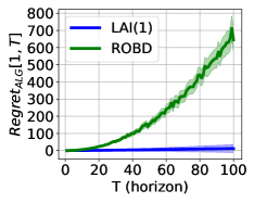
(a) light tail with $\lambda_{i}^{A}=0.3^{i-1}$

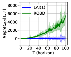
(b) log-normal with $\lambda_{i}^{A}=0.3^{i-1}$

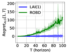
(c) pareto with $\lambda_{i}^{A}=0.3^{i-1}$

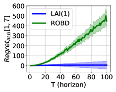
(d) light tail with $\lambda_{i}^{A}=0.5^{i-1}$

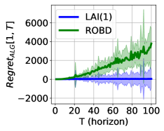
(e) log-normal with $\lambda_{i}^{A}=0.5^{i-1}$

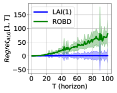
(f) pareto with $\lambda_{i}^{A}=0.5^{i-1}$

Figure 1: Regret of lai(1) and robd for martingale minimizers with light and heavy tails

The trends in Fig. 1 validate our claims in Theorem 3.6 and Theorem 3.12 (i) regarding robd’s linear regret and lai(1)’s constant regret. In fact, we observe that the regret of lai(1) is virtually zero in contrast to that of robd, demonstrating the superiority of lai$(\gamma)$ in practice. The insensitivity of lai$(\gamma)$ to the form of the distribution is further highlighted by its consistent near-optimal stochastic performance in all simulated stochastic settings. In particular, we would like to stress the stability demonstrated by lai$(\gamma)$ under shifting distributions and in heavy-tailed stochastic environments. The negligible regret shown by lai(1) establishes the superiority of lai$(\gamma)$ over robd in any distribution with finite variance.

4.2 Experiments in stochastic and adversarial environments

In this series of experiments, we introduce adversarial minimizers into a martingale minimizer sequence, with the extent of adversarial influence determined by the parameter known as the adversarial percentage denoted $(p)$. This parameter spans from $0$ (indicating a fully stochastic scenario) to $100$ (representing a fully adversarial scenario). To facilitate meaningful comparisons across stochastic and adversarial environments, we calculated the ratio of an online algorithm’s total cost to that of lai. This normalization technique helps account for the differences in the orders of magnitude between the total costs in stochastic and adversarial settings, allowing us to evaluate the relative performance of various algorithms effectively.

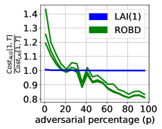
(a) normal to adversarial

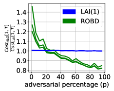
(b) log-normal to adversarial

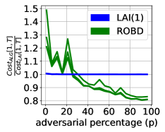
(c) pareto to adversarial

Figure 2: Behavior of lai(1) and robd for a mixed sequence of minimizers. In each figure, the topmost plot corresponds to $\left\{0.3^{i}\right\}_{i=0}^{9}$, the middle one represents $\left\{0.45^{i}\right\}_{i=0}^{9}$, and the bottom-most plot pertains to $\left\{0.5^{i}\right\}_{i=0}^{9}$.

In these experiments, we explore scenarios involving three different sequences of eigenvalues: $\left\{0.3^{i}\right\}_{i=0}^{9}$, $\left\{0.45^{i}\right\}_{i=0}^{9}$, and $\left\{0.5^{i}\right\}_{i=0}^{9}$. The key observation is that, on the adversarial end, the relative performance of lai(1) and robd is consistent across different $A$ matrices. However, it becomes evident that the stochastic performance of robd deteriorates significantly when a smaller $A$ matrix is used.

As we gradually intensify the adversarial characteristics of the environment, we notice a relatively smooth shift from lai(1) to robd in terms of identifying the “superior algorithm." In fact, until a certain threshold of adversarial influence, approximately around $20$%, lai(1) surpasses robd in performance. This intriguing observation prompts a more in-depth analysis of CFC in a stochastic environment with adversarial contamination.

5 Proofs

In this section, we shed light on the analysis techniques employed in this work, through detailed proofs of some of our main contributions. These include the stochastic optimality of lai, the poor performance of robd algorithm, the near-optimality of lai$(\gamma)$ in the stochastic setting, and our general adversarial analysis framework.

5.1 Proofs of Theorems 3.1 and 3.2

To prove these results, we show that lai is a dynamic programming solution in our stochastic setting (2.1); thus proving it to be an optimal online algorithm. The first step is to show the optimality of the action at round $T$, given by the following lemma.

Lemma 5.1.

The online optimal action at round $T$ is

$$x^{{\textsc{lai}}{}}_{T}=C_{T}x^{{\textsc{lai}}{}}_{T-1}+\left(I-C_{T}\right)v_{T}$$

and, consequently, the value function (2.3) for round $T$ is

$$V_{T}\left(x^{{\textsc{lai}}{}}_{T-1},v_{T}\right)=\frac{1}{2}\left(x^{{\textsc{lai}}{}}_{T-1}-v_{T}\right)^{T}\left(I-C_{T}\right)\left(x^{{\textsc{lai}}{}}_{T-1}-v_{T}\right)$$

We defer the proof of this to Appendix B.3 as it follows a simple derivative argument. We next present the main element of the proof of lai’s optimality in the form of the following proposition, from which Theorem 3.1 directly follows.

Proposition 5.2.

Consider hitting costs $\frac{1}{2}(x-v_{t})^{T}A(x-v_{t})$ and switching cost is $\frac{1}{2}\|x_{t}-x_{t-1}\|_{2}^{2}$ with the sequence of minimizers being a martingale, that is (2.1). The exact value function at $T-t$ is

$$\begin{split}V_{T-t}(x^{{\textsc{lai}}{}}_{T-t-1},v_{T-t})=&\frac{1}{2}(x^{{\textsc{lai}}{}}_{T-t-1}-v_{T-t})^{T}(I-C_{T-t})(x^{{\textsc{lai}}{}}_{T-t-1}-v_{T-t})\\ &+\sum_{s=0}^{t-1}\frac{1}{2}\mathbb{E}\left[(v_{T-s}-v_{T-s-1})^{T}(I-C_{T-s})(v_{T-s}-v_{T-s-1})|\mathcal{F}_{T-t}\right]\end{split}$$

Proof.

The proof follows via an induction argument. The value function at round $T$, according to Lemma 5.1, is

$$V_{T}(x^{{\textsc{lai}}{}}_{T-1},v_{T})=\frac{1}{2}(x^{{\textsc{lai}}{}}_{T-1}-v_{T})^{T}\left(I-C_{T}\right)(x^{{\textsc{lai}}{}}_{T-1}-v_{T}).$$ (5.1)

The proposition is, therefore, true for $t=0$ (sum from $0$ to $-1$ is zero). Assuming the proposition for some $t\geq 0$, we have the optimal action at round $T-t-1$ as

$$\begin{split}x^{{\textsc{lai}}{}}_{T-t-1}=\operatorname*{\arg\!\min}_{x}&\bigg{\{}\frac{1}{2}(x-v_{T-t-1})^{T}A(x-v_{T-t-1})+\frac{1}{2}\|x-x^{{\textsc{lai}}{}}_{T-t-2}\|_{2}^{2}\\ &+\mathbb{E}[V_{T-t}(x,v_{T-t})|\mathcal{F}_{T-t-1}]\bigg{\}}\end{split}$$ (5.2)

$$\begin{split}=\operatorname*{\arg\!\min}_{x}&\bigg{\{}\frac{1}{2}(x-v_{T-t-1})^{T}A(x-v_{T-t-1})+\frac{1}{2}\|x-x^{{\textsc{lai}}{}}_{T-t-2}\|_{2}^{2}\\ &+\frac{1}{2}\mathbb{E}\left[(x-v_{T-t})^{T}(I-C_{T-t})(x-v_{T-t})|\mathcal{F}_{T-t-1}\right]\\ &+\sum_{s=0}^{t-1}\frac{1}{2}\mathbb{E}\left[(v_{T-s}-v_{T-s-1})^{T}(I-C_{T-s})(v_{T-s}-v_{T-s-1})|\mathcal{F}_{T-t-1}\right]\bigg{\}}\end{split}$$ (5.3)

$$\begin{split}=\operatorname*{\arg\!\min}_{x}&\bigg{\{}\frac{1}{2}(x-v_{T-t-1})^{T}(A+I-C_{T-t})(x-v_{T-t-1})+\frac{1}{2}\|x-x^{{\textsc{lai}}{}}_{T-t-2}\|_{2}^{2}\\ &+(x-v_{T-t-1})^{T}(I-C_{T-t})\mathbb{E}[v_{T-t-1}-v_{T-t}|\mathcal{F}_{T-t-1}]\\ &+\frac{1}{2}\mathbb{E}[(v_{T-t}-v_{T-t-1})^{T}(I-C_{T-t})(v_{T-t}-v_{T-t-1})|\mathcal{F}_{T-t-1}]\\ &+\sum_{s=0}^{t-1}\frac{1}{2}\mathbb{E}\left[(v_{T-s}-v_{T-s-1})^{T}(I-C_{T-s})(v_{T-s}-v_{T-s-1})|\mathcal{F}_{T-t-1}\right]\bigg{\}}\end{split}$$ (5.4)

$$\begin{split}=\operatorname*{\arg\!\min}_{x}&\bigg{\{}\frac{1}{2}(x-v_{T-t-1})^{T}(A+I-C_{T-t})(x-v_{T-t-1})+\frac{1}{2}\|x-x^{{\textsc{lai}}{}}_{T-t-2}\|_{2}^{2}\\ &+\sum_{s=0}^{t}\frac{1}{2}\mathbb{E}\left[(v_{T-s}-v_{T-s-1})^{T}(I-C_{T-s})(v_{T-s}-v_{T-s-1})|\mathcal{F}_{T-t-1}\right]\bigg{\}}\end{split}$$ (5.5)

Differentiating the objective of the optimization problem above, we get

$$(A+I-C_{T-t})(x-v_{T-t-1})+(x-x^{{\textsc{lai}}{}}_{T-t-2})=0$$ (5.6)

giving us the optimal action at round $T-t-1$ as

$$x^{{\textsc{lai}}{}}_{T-t-1} =(2I+A-C_{T-t})^{-1}x^{{\textsc{lai}}{}}_{T-t-2}+\left(I-(2I+A-C_{T-t})^{-1}\right)v_{T-t-1}$$ (5.7)

$$=C_{T-t-1}x^{{\textsc{lai}}{}}_{T-t-2}+\left(I-C_{T-t-1}\right)v_{T-t-1}$$ (5.8)

where the invertibility of $(2I+A-C_{T-t})$ is easy to prove and is provided in the appendix. This proves Theorem 3.1. Consequently, the value function at round $T-t-1$ as

$$\begin{split}V_{T-t-1}(x^{{\textsc{lai}}{}}_{T-t-2}&,v_{T-t-1})\\ =&\frac{1}{2}(x^{{\textsc{lai}}{}}_{T-t-1}-v_{T-t-1})^{T}A(x^{{\textsc{lai}}{}}_{T-t-1}-v_{T-t-1})+\frac{1}{2}\|x^{{\textsc{lai}}{}}_{T-t-1}-x^{{\textsc{lai}}{}}_{T-t-2}\|_{2}^{2}\\ &+\mathbb{E}[V_{T-t}(x^{{\textsc{lai}}{}}_{T-t-1},v_{T-t})|\mathcal{F}_{T-t-1}]\end{split}$$ (5.9)

$$\begin{split}=&\frac{1}{2}(x^{{\textsc{lai}}{}}_{T-t-2}-v_{T-t-1})^{T}C_{T-t-1}(C_{T-t-1}^{-1}-I)C_{T-t-1}(x^{{\textsc{lai}}{}}_{T-t-2}-v_{T-t-1})\\ &+\frac{1}{2}(x^{{\textsc{lai}}{}}_{T-t-2}-v_{T-t-1})^{T}(I-C_{T-t-1})^{2}(x^{{\textsc{lai}}{}}_{T-t-2}-v_{T-t-1})\\ &+\sum_{s=0}^{t}\frac{1}{2}\mathbb{E}\left[(v_{T-s}-v_{T-s-1})^{T}(I-C_{T-s})(v_{T-s}-v_{T-s-1})|\mathcal{F}_{T-t-1}\right]\end{split}$$ (5.10)

$$\begin{split}=&\frac{1}{2}(x^{{\textsc{lai}}{}}_{T-t-2}-v_{T-t-1})^{T}(I-C_{T-t-1})(x^{{\textsc{lai}}{}}_{T-t-2}-v_{T-t-1})\\ &+\sum_{s=0}^{t}\frac{1}{2}\mathbb{E}\left[(v_{T-s}-v_{T-s-1})^{T}(I-C_{T-s})(v_{T-s}-v_{T-s-1})|\mathcal{F}_{T-t-1}\right]\end{split}$$ (5.11)

proving the proposition through induction. The cost of lai algorithm, which is also the online optimal cost, is

$$\mathbb{E} \left[\text{Cost}_{\text{{{lai}}{}}}[1,T]\right]=\mathbb{E}[V_{1}(x_{0},v_{1})|\mathcal{F}_{0}]=\sum_{t=1}^{T}\frac{1}{2}\mathbb{E}\left[(v_{t}-v_{t-1})^{T}(I-C_{t})(v_{t}-v_{t-1})|\mathcal{F}_{0}\right]$$ (5.12)

where $\mathcal{F}_{0}$ is the trivial sigma field and $v_{0}=x_{0}$. The upper bound in terms of $C_{L}$ is a consequence of the following important observation.

Lemma 5.3.

The matrix sequence in lai algorithm, that is, $\{C_{t}\}_{t}$ and $C_{L}$ are related as

$$C_{L}\prec C_{1}\prec C_{2}\prec\ldots\prec C_{T-1}\prec C_{T}.$$

The proof follows from the recursion satisfied by $\{C_{t}\}_{t}$, that is, $C_{t-1}^{-1}=2I+A-C_{t}$ and the fact that $C_{L}$ is the stationary point of this recursion. Due to space constraints, we defer the proof to Appendix B.5. This completes the proof of Theorem 3.2. ∎

5.2 Proof of Theorem 3.8

We split the proof into four parts, one of which will present the exact characterization of the lower bound. The first step is the cost of the fi algorithm, as the stated in the proposition below.

Proposition 5.4.

The following is the expected cost of the fi algorithm, with matrix $C$ for martingale minimizers (2.1) with increments having same covariance matrix, $\Sigma$,

$$\mathbb{E}[\text{Cost}_{{\textsc{fi}}{}}[1,T]]\geq\sum_{t=1}^{T}\frac{1}{2}\mathbb{E}\left[(v_{t}-v_{t-1})^{T}\left(I-C^{2}\right)^{-1}(AC^{2}+\left(I-C\right)^{2})(v_{t}-v_{t-1})\right]-\left(\frac{\left(\lambda_{\max}^{C}\right)^{2}}{1-\left(\lambda_{\max}^{C}\right)^{2}}\right)\frac{\sigma^{2}}{2}$$

The proof of this involves an induction argument to get the cost of the last $t$ rounds, however, we defer the proof of this result to Appendix B.5 in light of page constraints. The next step is to compare it to the cost of the lai algorithm to get the following lower bound to the regret.

Theorem 5.5.

Consider the hitting costs, switching costs and stochastic setting (2.1) from the problem set-up with $(v_{t}-v_{t-1})$ having covariance matrix $\Sigma$. The following is the regret of the fi algorithm,

$$\begin{split}\mathbb{E}[Regret_{{\textsc{fi}}{}}[1,T]]\geq\frac{T}{2}\sum_{j\not\in Z}\left(w\left(\lambda_{j}^{A},\lambda_{j}^{C}\right)-\left(1-\lambda_{j}^{L}\right)\right)(e_{j}^{T}P^{T}\Sigma Pe_{j})-\left(\frac{\left(\lambda_{\max}^{C}\right)^{2}}{1-\left(\lambda_{\max}^{C}\right)^{2}}\right)\frac{\sigma^{2}}{2}.\end{split}$$

where $w(\alpha,c)=\frac{\alpha c^{2}+(1-c)^{2}}{1-c^{2}}$, $Z=\{i\in\{1,\ldots,d\}:\lambda_{i}^{C}=\lambda_{i}^{L}\}$, $P$ is the modal matrix of $A$ and, $\lambda_{j}^{A},\lambda_{j}^{C},\lambda_{j}^{L}$ are the $j^{th}$ eigenvalues of $A,C,C_{L}$ respectively.

We will be presenting the proof of this exact lower bound shortly, after arguing that this lower bound scales as $\Omega(T)$ under the conditions of Theorem 3.8. The following lemma shows that $\left(w\left(\lambda_{j}^{A},\lambda_{j}^{C}\right)-\left(1-\lambda_{j}^{L}\right)\right)>0\text{ }\forall\text{ }j\not\in Z.$

Lemma 5.6.

The minimum of $w(\alpha,c)$ has the following properties

$$\operatorname*{\arg\!\min}_{c\in[0,1]}w(\alpha,c)=\frac{\alpha+2-\sqrt{\alpha^{2}+4\alpha}}{2}=\frac{2}{\alpha+2+\sqrt{\alpha^{2}+4\alpha}}=c_{L}\ \text{ and }\ \min_{c\in[0,1]}w(\alpha,c)=1-c_{L}.$$

Lastly, we show $(e_{j}^{T}P^{T}\Sigma Pe_{j})>0$ for both cases of $\Sigma$. The term becomes the $j^{th}$ eigenvalue of $\Sigma$ when it has same eigenvectors as $A$. The condition on $\Sigma$, in this case, requires at least one of the $j^{th}$ $(j\not\in Z)$ eigenvalues to be strictly greater than zero, giving $\Omega(T)$ regret. For $\Sigma$ with eigenvalues different than that of $A$, we use the following important observation to get $\Omega(T)$ regret.

Lemma 5.7.

Consider $A=PD_{A}P^{T}$, where $D_{A}$ is a diagonal matrix and a random vector $u_{t}\in\mathbb{R}^{d}$ with covariance matrix $\Sigma$. Suppose $\Sigma$ has modal matrix $Q\neq P$. Then $P^{T}u_{t}$ satisfies

$$\mathbb{E}\left[e_{j}^{T}\left(P^{T}u_{t}u_{t}^{T}P\right)e_{j}\right]=e_{j}^{T}P^{T}\Sigma Pe_{j}>0\text{ }\forall\text{ }j,t$$

We prove this lemma in the appendix. Having established the $\Omega(T)$ regret of fi, we now prove the regret lower bound in Theorem 5.5.

Proof of Theorem 5.5.

We can write $A=PD_{A}P^{T}$, $C_{L}=PD_{L}P^{T}$ and $C=PDP^{T}$, where $P$ is the modal matrix of A and the middle matrix in each being the diagonal matrix of respective eigenvalues.

$$\begin{split}\mathbb{E}[&\text{Cost}_{{\textsc{fi}}{}}[1,T]]-\mathbb{E}[\text{Cost}_{\text{{{lai}}{}}}[1,T]]\\ \geq&\sum_{t=1}^{T}\frac{1}{2}\mathbb{E}\left[(v_{t}-v_{t-1})^{T}\left(I-C^{2}\right)^{-1}(AC^{2}+\left(I-C\right)^{2})(v_{t}-v_{t-1})\right]\\ &-\left(\frac{\left(\lambda_{\max}^{C}\right)^{2}}{1-\left(\lambda_{\max}^{C}\right)^{2}}\right)\frac{\sigma^{2}}{2}-\sum_{t=1}^{T}\mathbb{E}[(v_{t}-v_{t-1})^{T}(1-C_{L})(v_{t}-v_{t-1})]\end{split}$$ (5.13)

$$\begin{split}\geq&\sum_{t=1}^{T}\frac{1}{2}\mathbb{E}\left[(v_{t}-v_{t-1})^{T}P\left(\left(I-D^{2}\right)^{-1}(D_{A}D^{2}+\left(I-D\right)^{2})-(I-D_{L})\right)P^{T}(v_{t}-v_{t-1})\right]\\ &-\left(\frac{\left(\lambda_{\max}^{C}\right)^{2}}{1-\left(\lambda_{\max}^{C}\right)^{2}}\right)\frac{\sigma^{2}}{2}\end{split}$$ (5.14)

Observe that we can write

$$\left(I-D^{2}\right)^{-1} (D_{A}D^{2}+\left(I-D\right)^{2})-(I-D_{L})$$ (5.15)

$$=diag\left(w\left(\lambda_{1}^{A},\lambda_{1}^{C}\right)-\left(1-\lambda_{1}^{L}\right),\ldots,w\left(\lambda_{d}^{A},\lambda_{d}^{C}\right)-\left(1-\lambda_{d}^{L}\right)\right)$$ (5.16)

We define the set of indices $Z=\{i\in\{1,\ldots,d\}:\lambda_{i}^{C}=\lambda_{i}^{L}\}$. Now, using Lemma 5.6, $w\left(\lambda_{i}^{A},\lambda_{i}^{C}\right)-\left(1-\lambda_{i}^{L}\right)>0\text{ if }i\not\in Z\text{ and }w\left(\lambda_{i}^{A},\lambda_{i}^{C}\right)-\left(1-\lambda_{i}^{L}\right)=0\text{ if }i\in Z.$ There has to be $i$ such that $i\not\in Z$. Otherwise, $C$ and $C_{L}$ will have all eigenvalues and their corresponding eigenvectors same, making them equal. Denoting $P^{T}(v_{t}-v_{t-1})=y_{t}$, the gap of fi to lai is

$$\begin{split}Regret_{{\textsc{fi}}{}}[1,T]\geq&\sum_{t=1}^{T}\frac{1}{2}\mathbb{E}\left[y_{t}^{T}diag\left(w\left(\lambda_{1}^{A},\lambda_{1}^{C}\right)-\left(1-\lambda_{1}^{L}\right),\ldots,w\left(\lambda_{d}^{A},\lambda_{d}^{C}\right)-\left(1-\lambda_{d}^{L}\right)\right)y_{t}\right]\\ &-\left(\frac{\left(\lambda_{\max}^{C}\right)^{2}}{1-\left(\lambda_{\max}^{C}\right)^{2}}\right)\frac{\sigma^{2}}{2}\end{split}$$ (5.17)

$$\begin{split}=&\sum_{t=1}^{T}\frac{1}{2}\sum_{j\not\in Z}\left(w\left(\lambda_{j}^{A},\lambda_{j}^{C}\right)-\left(1-\lambda_{j}^{L}\right)\right)\mathbb{E}(y_{t})_{j}^{2}-\left(\frac{\left(\lambda_{\max}^{C}\right)^{2}}{1-\left(\lambda_{\max}^{C}\right)^{2}}\right)\frac{\sigma^{2}}{2}\end{split}$$ (5.18)

$$\begin{split}=&\frac{T}{2}\sum_{j\not\in Z}\left(w\left(\lambda_{j}^{A},\lambda_{j}^{C}\right)-\left(1-\lambda_{j}^{L}\right)\right)\mathbb{E}(y)_{j}^{2}-\left(\frac{\left(\lambda_{\max}^{C}\right)^{2}}{1-\left(\lambda_{\max}^{C}\right)^{2}}\right)\frac{\sigma^{2}}{2}\end{split}$$ (5.19)

For the case where $A$ and $\Sigma$ different eigenvectors, Lemma 5.7 shows that $\mathbb{E}(y)_{j}^{2}>0\text{ }\forall\text{ }j$, giving $\Omega(T)$ regret. Now, let’s consider the second case. We have $\Sigma=PD_{\Sigma}P^{T}$ giving us

$$\mathbb{E}(y)_{j}^{2} =e_{j}^{T}P^{T}\Sigma Pe_{j}=D_{\Sigma}(j,j)$$ (5.20)

and

$$\begin{split}Regret_{{\textsc{fi}}{}}[1,T]\geq\frac{T}{2}\sum_{j\not\in Z}\left(w\left(\lambda_{j}^{A},\lambda_{j}^{C}\right)-\left(1-\lambda_{j}^{L}\right)\right)D_{\Sigma}(j,j)-\left(\frac{\left(\lambda_{\max}^{C}\right)^{2}}{1-\left(\lambda_{\max}^{C}\right)^{2}}\right)\frac{\sigma^{2}}{2}.\end{split}$$ (5.21)

Now, $(D-D_{L})D_{\Sigma}=0_{d\times d}\implies(C_{{\textsc{robd}}{}}-C_{L})\Sigma=0_{d\times d}$. Therefore, the condition in the second case, that is, $(C-C_{L})\Sigma\neq 0_{d\times d}$ implies, $\bar{D}=(D-D_{L})D_{\Sigma}\neq 0_{d\times d}$, meaning, $\bar{D}(j,j)=0$ if $j\in Z$ and $\bar{D}(j,j)=\left(\lambda_{j}^{C}-\lambda_{j}^{L}\right)D_{\Sigma}(j,j)$ if $j\not\in Z$. For $\bar{D}\neq 0$, there has to be some $j\not\in Z$ such that $D_{\Sigma}(j,j)>0$ proving that fi has $\Omega(T)$ regret. ∎

5.3 Proof of Theorem 3.12 (i)

The analysis of the upper bound on the regret of lai$(\gamma)$ involves two key steps. The first is an upper bound on the cost of lai$(\gamma)$, as stated in the following proposition.

Proposition 5.8.

The total cost of lai$(\gamma)$ for martingale minimizers (2.1) is upper bounded as

$$\begin{split}\mathbb{E}[\text{Cost}_{{\textsc{lai}(\gamma)}{}}[1,T]]&\leq\frac{1}{2}\sum_{t=1}^{T}\mathbb{E}\left[(v_{t}-v_{t-1})^{T}(I-\tilde{C}_{t})(v_{t}-v_{t-1})\right].\end{split}$$ (5.22)

The proof of this proposition uses an induction argument by cleverly employing the recursion followed by $\{\tilde{C}_{t}\}_{t}$ and has been deferred to Appendix D.1. The second step uses the following key property exhibited by eigenvalues of $\{\tilde{C}_{t}\}_{t}$ of lai$(\gamma)$ and $\{C_{t}\}_{t}$ of lai.

Lemma 5.9.

The $i^{th}$ eigenvalue of lai$(\gamma)$’s $\tilde{C}_{t}$, that is $\tilde{\lambda}_{i}^{t}$, and the $i^{th}$ eigenvalue of lai’s $C_{t}$, that is, $\lambda_{i}^{t}$, are related in the following manner

$$\left(\lambda_{i}^{t}-\tilde{\lambda}_{i}^{t}\right) \leq\frac{\lambda_{i}^{A}}{2}\left(\left(1+\frac{4}{\lambda_{i}^{A}}\right)^{\frac{\gamma}{2}}-1\right)\left(\lambda_{i}^{T}\right)^{2(T-t+1)}$$

The proof of this lemma uses the recursion followed by both $\{\tilde{C}_{t}\}_{t}$ and $\{\tilde{C}_{t}\}_{t}$ and is presented in Appendix D.2. We now proceed to upper bound the regret of lai$(\gamma)$ algorithm.

Proof of Theorem 3.12.

We write each $C_{t}$ and $\tilde{C}_{t}$ as $PD_{t}P^{T}$ and $P\tilde{D}_{t}P^{T}$ where $D_{t}$ and $\tilde{D}_{t}$ are the eigenvalue diagonal matrices of $C_{t}$ and $\tilde{C}_{t}$ respectively. Therefore, regret of lai$(\gamma)$ is upper-bounded as

$$\mathbb{E}[Cost_{{\textsc{lai}(\gamma)}{}}[1,T]]-\mathbb{E}[\text{Cost}_{\text{{{lai}}{}}}[1,T]]\leq\frac{1}{2}\sum_{t=1}^{T}\mathbb{E}\left[(v_{t}-v_{t-1})^{T}(C_{t}-\tilde{C}_{t})(v_{t}-v_{t-1})\right]$$ (5.23)

$$=\frac{1}{2}\sum_{t=1}^{T}\mathbb{E}\left[(v_{t}-v_{t-1})^{T}P(D_{t}-\tilde{D}_{t})P^{T}(v_{t}-v_{t-1})\right]\leq\frac{1}{2}\sum_{t=1}^{T}\sum_{i=1}^{d}\left(\lambda_{i}^{t}-\tilde{\lambda}_{i}^{t}\right)\mathbb{E}(y_{t})_{i}^{2}$$ (5.24)

$$=\frac{1}{2}\sum_{i=1}^{d}\mathbb{E}(y)_{i}^{2}\sum_{t=1}^{T}\left(\lambda_{i}^{t}-\tilde{\lambda}_{i}^{t}\right)\leq\frac{1}{2}\sum_{i=1}^{d}\mathbb{E}(y)_{i}^{2}\sum_{t=1}^{T}\frac{\lambda_{i}^{A}}{2}\left(\left(1+\frac{4}{\lambda_{i}^{A}}\right)^{\frac{\gamma}{2}}-1\right)\left(\lambda_{i}^{T}\right)^{2(T-t+1)}$$ (5.25)

$$\leq\frac{1}{2}\sum_{i=1}^{d}\mathbb{E}(y)_{i}^{2}\frac{\lambda_{i}^{A}}{2}\left(\left(1+\frac{4}{\lambda_{i}^{A}}\right)^{\frac{\gamma}{2}}-1\right)\sum_{t=1}^{\infty}\left(\lambda_{i}^{T}\right)^{2t}=\frac{1}{2}\sum_{i=1}^{d}\mathbb{E}(y)_{i}^{2}\frac{\lambda_{i}^{A}}{2}\left(\left(1+\frac{4}{\lambda_{i}^{A}}\right)^{\frac{\gamma}{2}}-1\right)\frac{\left(\lambda_{i}^{T}\right)^{2}}{1-\left(\lambda_{i}^{T}\right)^{2}}$$ (5.26)

$$=\frac{1}{2}\sum_{i=1}^{d}\mathbb{E}(y)_{i}^{2}\frac{\left(\left(1+\frac{4}{\lambda_{i}^{A}}\right)^{\frac{\gamma}{2}}-1\right)}{2\left(\lambda_{i}^{A}+2\right)}$$ (5.27)

where $y_{t}=P^{T}(v_{t}-v_{t-1})$. Note that $\mathbb{E}(y_{t})_{i}^{2}=\mathbb{E}(y)_{i}^{2}$ is time-invariant as all $(v_{t}-v_{t-1})$ have same covariance $\Sigma$. The function $\left(\left(1+\frac{4}{q}\right)^{\frac{\gamma}{2}}-1\right)/(2\left(q+2\right))$ is always decreasing in $q$ for $\gamma\in[0,1]$. Therefore,

$$\text{Regret}_{{\textsc{lai}(\gamma)}{}}[1,T]\leq\frac{1}{4}\frac{\left(\left(1+\frac{4}{\lambda_{\min}^{A}}\right)^{\frac{\gamma}{2}}-1\right)}{\left(\lambda_{\min}^{A}+2\right)}\sum_{i=1}^{d}\mathbb{E}(y)_{i}^{2}=\frac{\left(\left(1+\frac{4}{\lambda_{\min}^{A}}\right)^{\frac{\gamma}{2}}-1\right)}{\left(\lambda_{\min}^{A}+2\right)}\frac{\sigma^{2}}{4}$$ (5.29)

where the last step uses $\sum_{i=1}^{d}\mathbb{E}(y)_{i}^{2}=\sigma^{2}=tr(\Sigma)$ which can be easily proved (in the appendix). ∎

5.4 Proof of Theorem 3.11

The proof technique used here is inspired from robd’s competitive analysis in [16]. The key aspect of our proof is the potential function that depends on $g_{t}(\cdot)$ of the online algorithm alg in question. To recap, the online algorithm alg is

$$x_{t}=\operatorname*{\arg\!\min}_{x}f_{t}(x)+D_{h}(x||x_{t-1})+D_{g_{t}}(x||v_{t})$$ (5.30)

where $f_{t}$ is $m$-strongly convex and $h(\cdot)$ is $\alpha$-strongly convex and $\beta$-smooth. Recall that $g_{t}(\cdot)$ is $\alpha^{\prime}-$strongly convex and $\beta^{\prime}-$smooth. This means

$$\nabla f_{t}(x_{t})+(\nabla h(x_{t})-\nabla h(x_{t-1}))+(\nabla g_{t}(x_{t})-\nabla g_{t}(v_{t}))=0.$$ (5.31)

We denote the hindsight optimal action sequence as $\left\{x_{t}^{*}\right\}_{t}$. Using strong convexity of $f_{t}$

$$f_{t}(x_{t}^{*})\geq f_{t}(x_{t})+\langle\nabla f_{t}(x_{t}),x_{t}^{*}-x_{t}\rangle+\frac{m}{2}\left\|x_{t}^{*}-x_{t}\right\|_{2}^{2}$$ (5.32)

$$= f_{t}(x_{t})-\langle\nabla h(x_{t-1})-\nabla h(x_{t}),x_{t}-x_{t}^{*}\rangle$$ (5.33)

$$-\langle\nabla g_{t}(v_{t})-\nabla g_{t}(x_{t}),x_{t}-x_{t}^{*}\rangle+\frac{m}{2}\left\|x_{t}^{*}-x_{t}\right\|_{2}^{2}.$$ (5.34)

Using the general triangle inequality for Bregman divergence (Lemma D.3), for $D_{h}\left(\cdot||\cdot\right)$ and $D_{g_{t}}\left(\cdot||\cdot\right)$, we have

$$\langle\nabla h(x_{t-1})-\nabla h(x_{t}),x_{t}-x_{t}^{*}\rangle=D_{h}(x_{t}^{*}||x_{t-1})-D_{h}(x_{t}^{*}||x_{t})-D_{h}(x_{t}||x_{t-1})$$ (5.35)

and

$$\langle\nabla g_{t}(v_{t})-\nabla g_{t}(x_{t}),x_{t}-x_{t}^{*}\rangle=D_{g_{t}}(x_{t}^{*}||v_{t})-D_{g_{t}}(x_{t}^{*}||x_{t})-D_{g_{t}}(x_{t}||v_{t}).$$ (5.36)

Substituting the two above identities into inequality (5.34), we get

$$f_{t}(x_{t})+D_{h}(x_{t}||x_{t-1})+(D_{h}(x_{t}^{*}||x_{t})+D_{g_{t}}(x_{t}^{*}||x_{t}))+\frac{m}{2}\left\|x_{t}^{*}-x_{t}\right\|_{2}^{2}+D_{g_{t}}(x_{t}||v_{t})$$ (5.37)

$$\leq f_{t}(x_{t}^{*})+D_{g_{t}}(x_{t}^{*}||v_{t})+D_{h}(x_{t}^{*}||x_{t-1})$$ (5.38)

It follows that

$$\begin{split}&f_{t}(x_{t})+D_{h}(x_{t}||x_{t-1})+(D_{h}(x_{t}^{*}||x_{t})+D_{g_{t}}(x_{t}^{*}||x_{t}))+\frac{m}{2}\left\|x_{t}^{*}-x_{t}\right\|_{2}^{2}\\ &\leq f_{t}(x_{t}^{*})+D_{g_{t}}(x_{t}^{*}||v_{t})+D_{h}(x_{t}^{*}||x_{t-1})\end{split}$$ (5.39)

Now, define the potential function $\phi(x_{t},x_{t}^{*})=(D_{h}(x_{t}^{*}||x_{t})+D_{g_{t}}(x_{t}^{*}||x_{t}))+\frac{m}{2}\left\|x_{t}^{*}-x_{t}\right\|_{2}^{2}$ and the potential difference as $\Delta\phi=\phi(x_{t},x_{t}^{*})-\phi(x_{t-1},x_{t-1}^{*})$. Subtracting $\phi(x_{t-1},x_{t-1}^{*})$ from both sides of the above inequality, we get

$$\begin{split}&f_{t}(x_{t})+D_{h}(x_{t}||x_{t-1})+\Delta\phi\\ &\leq\underbrace{(f_{t}(x_{t}^{*})+D_{g_{t}}(x_{t}^{*}||v_{t}))}_{X_{1}}+\underbrace{D_{h}(x_{t}^{*}||x_{t-1})-(D_{h}(x_{t-1}^{*}||x_{t-1})+D_{g_{t-1}}(x_{t-1}^{*}||x_{t-1}))-\frac{m}{2}\left\|x_{t-1}^{*}-x_{t-1}\right\|_{2}^{2}}_{X_{2}}\end{split}$$ (5.40)

We now analyze $X_{2}$

$$D_{h}( x_{t}^{*}||x_{t-1})-\left(D_{h}(x_{t-1}^{*}||x_{t-1})+D_{g_{t-1}}(x_{t-1}^{*}||x_{t-1})\right)-\frac{m}{2}\left\|x_{t-1}^{*}-x_{t-1}\right\|_{2}^{2}$$ (5.41)

$$= \text{ }(D_{h}(x_{t}^{*}||x_{t-1})-D_{h}(x_{t-1}^{*}||x_{t-1}))-D_{g_{t-1}}(x_{t-1}^{*}||x_{t-1})-\frac{m}{2}\left\|x_{t-1}^{*}-x_{t-1}\right\|_{2}^{2}$$ (5.42)

$$\begin{split}=&\text{ }D_{h}(x_{t}^{*}||x_{t-1}^{*})+\langle\nabla h(x_{t-1})-\nabla h(x_{t-1}^{*}),x_{t-1}^{*}-x_{t}^{*}\rangle-D_{g_{t-1}}(x_{t-1}^{*}||x_{t-1})-\frac{m}{2}\left\|x_{t-1}^{*}-x_{t-1}\right\|_{2}^{2}\end{split}$$ (5.43)

$$\begin{split}\leq&\text{ }D_{h}(x_{t}^{*}||x_{t-1}^{*})+\|\nabla h(x_{t-1})-\nabla h(x_{t-1}^{*})\|_{2}\|x_{t-1}^{*}-x_{t}^{*}\|_{2}-D_{g_{t-1}}(x_{t-1}^{*}||x_{t-1})-\frac{m}{2}\left\|x_{t-1}^{*}-x_{t-1}\right\|_{2}^{2}\end{split}$$ (5.44)

$$\begin{split}\leq&\text{ }D_{h}(x_{t}^{*}||x_{t-1}^{*})+\beta\|x_{t-1}-x_{t-1}^{*}\|_{2}\|x_{t-1}^{*}-x_{t}^{*}\|_{2}-D_{g_{t-1}}(x_{t-1}^{*}||x_{t-1})-\frac{m}{2}\left\|x_{t-1}^{*}-x_{t-1}\right\|_{2}^{2}\end{split}$$ (5.45)

$$\begin{split}\leq&\text{ }D_{h}(x_{t}^{*}||x_{t-1}^{*})+\frac{1}{2}\left(\frac{\beta^{2}}{\alpha^{\prime}_{t-1}+m}\right)\|x_{t-1}^{*}-x_{t}^{*}\|_{2}^{2}+\left(\frac{\alpha^{\prime}+m}{2}\right)\|x_{t-1}-x_{t-1}^{*}\|_{2}^{2}\\ &-D_{g_{t-1}}(x_{t-1}^{*}||x_{t-1})-\frac{m}{2}\left\|x_{t-1}^{*}-x_{t-1}\right\|_{2}^{2}\end{split}$$ (5.46)

$$\begin{split}=&\text{ }D_{h}(x_{t}^{*}||x_{t-1}^{*})+\frac{1}{2}\left(\frac{\beta^{2}}{\alpha^{\prime}_{t-1}+m}\right)\|x_{t-1}^{*}-x_{t}^{*}\|_{2}^{2}+\left(\frac{\alpha^{\prime}_{t-1}}{2}\|x_{t-1}-x_{t-1}^{*}\|_{2}^{2}-D_{g_{t-1}}(x_{t-1}^{*}||x_{t-1})\right)\end{split}$$ (5.47)

$$\begin{split}\leq&\text{ }D_{h}(x_{t}^{*}||x_{t-1}^{*})+\frac{1}{2}\left(\frac{\beta^{2}}{\alpha^{\prime}_{t-1}+m}\right)\|x_{t-1}^{*}-x_{t}^{*}\|_{2}^{2}\end{split}\leq\left(1+\frac{\beta^{2}/\alpha}{\alpha^{\prime}_{t-1}+m}\right)D_{h}(x_{t}^{*}||x_{t-1}^{*})$$ (5.48)

Therefore,

$$f_{t}(x_{t})+D_{h}(x_{t}||x_{t-1})+\Delta\phi \leq f_{t}(x_{t}^{*})+D_{g_{t}}(x_{t}^{*}||v_{t})+\left(1+\frac{\beta^{2}/\alpha}{\alpha^{\prime}_{t-1}+m}\right)D_{h}(x_{t}^{*}||x_{t-1}^{*})$$ (5.49)

$$\leq f_{t}(x_{t}^{*})+\frac{\beta^{\prime}_{t}}{2}\|x_{t}^{*}-v_{t}\|^{2}+\left(1+\frac{\beta^{2}/\alpha}{\alpha^{\prime}_{t-1}+m}\right)D_{h}(x_{t}^{*}||x_{t-1}^{*})$$ (5.50)

$$=\left(1+\frac{\beta^{\prime}_{t}}{m}\right)f_{t}(x_{t}^{*})+\left(1+\frac{\beta^{2}/\alpha}{\alpha^{\prime}_{t-1}+m}\right)D_{h}(x_{t}^{*}||x_{t-1}^{*})$$ (5.51)

$$\leq\left(1+\frac{\max_{t}\beta^{\prime}_{t}}{m}\right)f_{t}(x_{t}^{*})+\left(1+\frac{\beta^{2}/\alpha}{\min_{t}\alpha^{\prime}_{t-1}+m}\right)D_{h}(x_{t}^{*}||x_{t-1}^{*})$$ (5.52)

∎

6 Concluding Remarks

In this work, we address the Convex Function Chasing (CFC) problem within both stochastic and adversarial scenarios, offering contributions in both settings. We provide the first comprehensive stochastic characterization of CFC under quadratic costs and martingale minimizers, resulting in the stochastic online optimal algorithm, lai. We establish the fundamental disparities between the stochastic and adversarial settings in CFC by proving two results: the linear regret for the adversarial optimal algorithm compared to lai in the stochastic setting and the sup-optimal competitive ratio of lai in the adversarial setting. Additionally, we break through the apparent trade-off between the two settings by introducing a novel best-of-both-worlds algorithm, lai$(\gamma)$, which achieves near-optimal competitive ratio in the adversarial setting while maintaining only a constant regret compared to the stochastic optimal. In addition to these, we provide two results that go beyond the primary setting considered in this work. On the stochastic front, we generalize the stochastic optimal algorithm to the broader class of models that allows for martingales with non-zero drift. On the adversarial front, we provide an analysis framework that accommodates a large class of algorithms and cost settings, going beyond the adversarial results for lai and lai$(\gamma)$.

This research broadens the horizons of CFC in two unexplored dimensions: the examination of CFC within stochastic contexts and the concept of “best of both worlds" algorithms for CFC problems. These directions hold immense potential, spanning from extending the stochastic analysis beyond quadratic costs, to investigating diverse random processes governing the minimizer sequence. Within the framework discussed in this work, one particularly intriguing problem is to devise strategies to address the challenges posed by the lack of knowledge of the matrix $A$ in the hitting cost or the drift coefficient in the minimizer.

Appendix A Lazy Adaptive Interpolation for maringale minimizers with drift

We extend the stochastic analysis of the CFC framework to the following stochastic setting for any $b\in\mathbb{R}^{d}$

$$\mathbb{E}[v_{s}|\mathcal{F}_{t}]=v_{t}+(s-t)b\text{ }\forall\text{ }s\geq t.$$ (A.1)

We develop the online optimal stochastic algorithm for this setting by carefully studying the influence of drift on the mechanics of the dynamic programming method in this context and present Algorithm 3 as the best action sequence possible online.

Algorithm 3 Lazy Adaptive Interpolation with drift

The complex structure of the drift component in $x^{LAI}_{t}$ is deciphered in an inductive fashion by observing patterns in this problem’s DP formulation. We prove that the online action in Algorithm 3, with the specific drift addition, is the stochastic optimal in the following result.

Theorem A.1.

Consider hitting costs $f_{t}(x)=\frac{1}{2}(x-v_{t})^{T}A(x-v_{t})$ and switching cost is $c(x_{t},x_{t-1})=\frac{1}{2}\|x_{t}-x_{t-1}\|_{2}^{2}$ with the minimizers evolving as a martingale with drift $b\in\mathbb{R}^{d}$ (A.1). The value function (2.3) at round $T-t$ is

$$V_{T-t}(x^{{\textsc{lai}}{}}_{T-t-1},v_{T-t})=\begin{cases}(1/2)(x^{{\textsc{lai}}{}}_{T-1}-v_{T})^{T}(I-C_{T})(x^{{\textsc{lai}}{}}_{T-1}-v_{T})&t=0\\ \begin{split}(&1/2)(x^{{\textsc{lai}}{}}_{T-t-1}-v_{T-t})^{T}(I-C_{T-t})(x^{{\textsc{lai}}{}}_{T-t-1}-v_{T-t})\\ &-(x^{{\textsc{lai}}{}}_{T-t-1}-v_{T-t})^{T}C_{T-t}\left(I-\prod_{s=t-1}^{0}C_{T-s}\right)b+a_{T-t}\end{split}&t\geq 1\end{cases}$$

where $a_{T-t}$ is a constant independent of $x^{{\textsc{lai}}{}}_{T-t-1}$. Consequently, the online optimal action at round $T-t-1$ is

$$x^{{\textsc{lai}}{}}_{T-t-1}=C_{T-t-1}x^{{\textsc{lai}}{}}_{T-t-2}+(I-C_{T-t-1})v_{T-t-1}+C_{T-t-1}\left(I-\prod_{s=t}^{0}C_{T-s}\right)b$$

with the online optimal action at round $T$ being $x^{{\textsc{lai}}{}}_{T}=C_{T}x^{{\textsc{lai}}{}}_{T-t-1}+(1-C_{T})v_{T}$.

Proof.

The proof follows an induction argument. Notice that, given the penultimate action $x^{{\textsc{lai}}{}}_{T-1}$ and the final minimizer $v_{T}$, the online optimal action at the last round $T$ and the associated cost-to-go (which, in this case, is the cost of the final round) is given by Lemma 5.1. Therefore, the value function of the final round is

$$V_{T}(x^{{\textsc{lai}}{}}_{T-1},v_{T})=\frac{1}{2}(x^{{\textsc{lai}}{}}_{T-1}-v_{T})^{T}\left(I-C_{T}\right)(x^{{\textsc{lai}}{}}_{T-1}-v_{T}).$$ (A.2)

Therefore, at round $T-1$, the decision is

$$x^{{\textsc{lai}}{}}_{T-1}=\operatorname*{\arg\!\min}_{x}\bigg{\{} \frac{1}{2}(x-v_{T-1})^{T}A(x-v_{T-1})+\frac{1}{2}\|x-x^{{\textsc{lai}}{}}_{T-2}\|_{2}^{2}+\mathbb{E}\left[V_{T}(x,v_{T})|\mathcal{F}_{T-1}\right]\bigg{\}}$$ (A.3)

$$\begin{split}=\operatorname*{\arg\!\min}_{x}\bigg{\{}&\frac{1}{2}(x-v_{T-1})^{T}A(x-v_{T-1})+\frac{1}{2}\|x-x^{{\textsc{lai}}{}}_{T-2}\|_{2}^{2}+\frac{1}{2}(x-v_{T-1})^{T}\left(I-C_{T}\right)(x-v_{T-1})\\ &+(x-v_{T-1})^{T}(I-C_{T})\mathbb{E}\left[v_{T-1}-v_{T}|\mathcal{F}_{T-1}\right]\\ &+\frac{1}{2}\mathbb{E}\left[(v_{T-1}-v_{T})^{T}(I-C_{T})(v_{T-1}-v_{T})|\mathcal{F}_{T-1}\right]\bigg{\}}\end{split}$$ (A.4)

$$\begin{split}=\operatorname*{\arg\!\min}_{x}\bigg{\{}&\frac{1}{2}(x-v_{T-1})^{T}(I+A-C_{T})(x-v_{T-1})+\frac{1}{2}\|x-x^{{\textsc{lai}}{}}_{T-2}\|_{2}^{2}-(x-v_{T-1})^{T}(I-C_{T})b\bigg{\}}\end{split}$$ (A.5)

Differentiating with respect to $x$, we get

$$(2I+A-C_{T})x=x^{{\textsc{lai}}{}}_{T-2}+(I+A-C_{T})v_{T-1}+(I-C_{T})b$$ (A.6)

which gives the decision as

$$x^{{\textsc{lai}}{}}_{T-1} =(2I+A-C_{T})^{-1}x^{{\textsc{lai}}{}}_{T-2}+(2I+A-C_{T})^{-1}(I+A-C_{T})v_{T-1}+(2I+A-C_{T})^{-1}(I-C_{T})b$$ (A.7)

$$=(2I+A-C_{T})^{-1}x^{{\textsc{lai}}{}}_{T-2}+(2I+A-C_{T})^{-1}(2I+A-C_{T}-I)v_{T-1}+(2I+A-C_{T})^{-1}(I-C_{T})b$$ (A.8)

$$=(2I+A-C_{T})^{-1}x^{{\textsc{lai}}{}}_{T-2}+(I-(2I+A-C_{T})^{-1})v_{T-1}+(2I+A-C_{T})^{-1}(I-C_{T})b$$ (A.9)

$$=C_{T-1}x^{{\textsc{lai}}{}}_{T-2}+(I-C_{T-1})v_{T-1}+C_{T-1}(I-C_{T})b.$$ (A.10)

Putting $x^{{\textsc{lai}}{}}_{T-1}$ back into the cost-to-go of round $T-1$ gives the value function at round $T-1$ as

$$\begin{split}V&(x^{{\textsc{lai}}{}}_{T-2},v_{T-1})\\ =&\frac{1}{2}(C_{T-1}(x^{{\textsc{lai}}{}}_{T-2}-v_{T-1})+C_{T-1}(I-C_{T})b)^{T}(I+A-C_{T})(C_{T-1}(x^{{\textsc{lai}}{}}_{T-2}-v_{T-1})+C_{T-1}(I-C_{T})b)\\ &+\frac{1}{2}((I-C_{T-1})(v_{T-1}-x^{{\textsc{lai}}{}}_{T-2})+C_{T-1}(I-C_{T})b)^{T}((I-C_{T-1})(v_{T-1}-x^{{\textsc{lai}}{}}_{T-2})+C_{T-1}(I-C_{T})b)\\ &-(C_{T-1}(x^{{\textsc{lai}}{}}_{T-2}-v_{T-1})+C_{T-1}(I-C_{T})b)^{T}(I-C_{T})b\\ &+\frac{1}{2}\mathbb{E}\left[(v_{T-1}-v_{T})^{T}(I-C_{T})(v_{T-1}-v_{T})|\mathcal{F}_{T-1}\right]\end{split}$$ (A.11)

$$\begin{split}=&\frac{1}{2}(x^{{\textsc{lai}}{}}_{T-2}-v_{T-1})^{T}C_{T-1}(C_{T-1}^{-1}-I)C_{T-1}(x^{{\textsc{lai}}{}}_{T-2}-v_{T-1})+\frac{1}{2}(v_{T-1}-x^{{\textsc{lai}}{}}_{T-2})^{T}(I-C_{T-1})^{2}(v_{T-1}-x^{{\textsc{lai}}{}}_{T-2})\\ &+(b^{T}(I-C_{T})C_{T-1})(C_{T-1}^{-1}-I)C_{T-1}(x^{{\textsc{lai}}{}}_{T-2}-v_{T-1})+(b^{T}(I-C_{T})C_{T-1})(I-C_{T-1})(v_{T-1}-x^{{\textsc{lai}}{}}_{T-2})\\ &-(x^{{\textsc{lai}}{}}_{T-2}-v_{T-1})^{T}C_{T-1}(I-C_{T})b+b^{T}Q_{T-1}b+\frac{1}{2}\mathbb{E}\left[(v_{T-1}-v_{T})^{T}(I-C_{T})(v_{T-1}-v_{T})|\mathcal{F}_{T-1}\right]\end{split}$$ (A.12)

$$\begin{split}=&\frac{1}{2}(x^{{\textsc{lai}}{}}_{T-2}-v_{T-1})^{T}\left((I-C_{T-1})C_{T-1}+(I-C_{T-1})^{2}\right)(x^{{\textsc{lai}}{}}_{T-2}-v_{T-1})\\ &-(x^{{\textsc{lai}}{}}_{T-2}-v_{T-1})^{T}C_{T-1}(I-C_{T})b+a_{T-1}\end{split}$$ (A.13)

$$\begin{split}=&\frac{1}{2}(x^{{\textsc{lai}}{}}_{T-2}-v_{T-1})^{T}(I-C_{T-1})(x^{{\textsc{lai}}{}}_{T-2}-v_{T-1})-(x^{{\textsc{lai}}{}}_{T-2}-v_{T-1})^{T}C_{T-1}(I-C_{T})b+a_{T-1}\end{split}$$ (A.14)

where, $b^{T}Q_{T-1}b$ is an accumulation of all terms of the form $b^{T}Mb$. Naturally, these terms are constants with respect to $x^{{\textsc{lai}}{}}_{T-2}$ and have, therefore, been clubbed together into $a_{T-1}$. Therefore, the claim holds for $t=1$. Assuming that the claim holds for some $t\geq 1$,

$$\begin{split}\mathbb{E}[V_{T-t}(x^{{\textsc{lai}}{}}_{T-t-1},&v_{T-t})|\mathcal{F}_{T-t-1}]\\ =&\frac{1}{2}\mathbb{E}\left[(x^{{\textsc{lai}}{}}_{T-t-1}-v_{T-t})^{T}(I-C_{T-t})(x^{{\textsc{lai}}{}}_{T-t-1}-v_{T-t})|\mathcal{F}_{T-t-1}\right]\\ &-\mathbb{E}\left[(x^{{\textsc{lai}}{}}_{T-t-1}-v_{T-t})|\mathcal{F}_{T-t-1}\right]^{T}C_{T-t}\left(I-\prod_{s=t-1}^{0}C_{T-s}\right)b+\mathbb{E}[a_{T-t}|\mathcal{F}_{T-t-1}]\end{split}$$ (A.15)

$$\begin{split}=&\frac{1}{2}(x^{{\textsc{lai}}{}}_{T-t-1}-v_{T-t-1})^{T}(I-C_{T-t})(x^{{\textsc{lai}}{}}_{T-t-1}-v_{T-t-1})\\ &+(x^{{\textsc{lai}}{}}_{T-t-1}-v_{T-t-1})^{T}(I-C_{T-t})\mathbb{E}[v_{T-t-1}-v_{T-t}|\mathcal{F}_{T-t-1}]\\ &+\frac{1}{2}\mathbb{E}[(v_{T-t-1}-v_{T-t})^{T}(I-C_{T-t})(v_{T-t-1}-v_{T-t})|\mathcal{F}_{T-t-1}]\\ &-(x^{{\textsc{lai}}{}}_{T-t-1}-v_{T-t-1}-b)^{T}C_{T-t}\left(I-\prod_{s=t-1}^{0}C_{T-s}\right)b+\mathbb{E}[a_{T-t}|\mathcal{F}_{T-t-1}]\end{split}$$ (A.16)

$$\begin{split}=&\frac{1}{2}(x^{{\textsc{lai}}{}}_{T-t-1}-v_{T-t-1})^{T}(I-C_{T-t})(x^{{\textsc{lai}}{}}_{T-t-1}-v_{T-t-1})\\ &-(x^{{\textsc{lai}}{}}_{T-t-1}-v_{T-t-1})^{T}(I-C_{T-t})b\\ &-(x^{{\textsc{lai}}{}}_{T-t-1}-v_{T-t-1})^{T}C_{T-t}\left(I-\prod_{s=t-1}^{0}C_{T-s}\right)b+\mathbb{E}[a^{\prime}_{T-t}|\mathcal{F}_{T-t-1}]\end{split}$$ (A.17)

$$\begin{split}=&\frac{1}{2}(x^{{\textsc{lai}}{}}_{T-t-1}-v_{T-t-1})^{T}(I-C_{T-t})(x^{{\textsc{lai}}{}}_{T-t-1}-v_{T-t-1})\\ &-(x^{{\textsc{lai}}{}}_{T-t-1}-v_{T-t-1})^{T}\left(I-\prod_{s=t}^{0}C_{T-s}\right)b+\mathbb{E}[a^{\prime}_{T-t}|\mathcal{F}_{T-t-1}].\end{split}$$ (A.18)

where $\mathbb{E}[a^{\prime}_{T-t}|\mathcal{F}_{T-t-1}]$ is also a constant with respect to $x^{{\textsc{lai}}{}}_{T-t-1}$. Therefore, the decision at round $T-t-1$ is

$$\begin{split}x^{{\textsc{lai}}{}}_{T-t-1}=\operatorname*{\arg\!\min}_{x}\bigg{\{}&\frac{1}{2}(x-v_{T-t-1})^{T}A(x-v_{T-t-1})+\frac{1}{2}\|x-x^{{\textsc{lai}}{}}_{T-t-2}\|_{2}^{2}\\ &+\mathbb{E}[V_{T-t}(x,v_{T-t})|\mathcal{F}_{T-t-1}]\bigg{\}}\end{split}$$ (A.19)

$$\begin{split}=\operatorname*{\arg\!\min}_{x}\bigg{\{}&\frac{1}{2}(x-v_{T-t-1})^{T}(I+A-C_{T-t})(x-v_{T-t-1})+\frac{1}{2}\|x-x^{{\textsc{lai}}{}}_{T-t-2}\|_{2}^{2}\\ &-(x-v_{T-t-1})^{T}\left(I-\prod_{s=t}^{0}C_{T-s}\right)b+\mathbb{E}[a^{\prime}_{T-t}|\mathcal{F}_{T-t-1}]\bigg{\}}\end{split}$$ (A.20)

Equating the derivative of the objective to zero gives,

$$(2I+A-C_{T-t})x=x^{{\textsc{lai}}{}}_{T-t-2}+(I+A-C_{T-t})v_{T-t-1}+\left(I-\prod_{s=t}^{0}C_{T-s}\right)b$$ (A.21)

which gives the online optimal action at round $(T-t-1)$ as

$$\begin{split}x^{{\textsc{lai}}{}}_{T-t-1}=&(2I+A-C_{T-t})^{-1}x^{{\textsc{lai}}{}}_{T-t-2}+(2I+A-C_{T-t})^{-1}(I+A-C_{T-t})v_{T-t-1}\\ &+(2I+A-C_{T-t})^{-1}\left(I-\prod_{s=t}^{0}C_{T-s}\right)b\end{split}$$ (A.22)

$$= C_{T-t-1}x^{{\textsc{lai}}{}}_{T-t-2}+C_{T-t-1}(C_{T-t-1}^{-1}-I)v_{T-t-1}+C_{T-t-1}\left(I-\prod_{s=t}^{0}C_{T-s}\right)b$$ (A.23)

$$= C_{T-t-1}x^{{\textsc{lai}}{}}_{T-t-2}+(I-C_{T-t-1})v_{T-t-1}+C_{T-t-1}\left(I-\prod_{s=t}^{0}C_{T-s}\right)b$$ (A.24)

We put this into the lai objective of round $T-t-1$ to get the value function of this round

$$\begin{split}V_{T-t-1}(&x^{{\textsc{lai}}{}}_{T-t-2},v_{T-t-1})\\ =&\frac{1}{2}\left(C_{T-t-1}\left(x^{{\textsc{lai}}{}}_{T-t-2}-v_{T-t-1}\right)+C_{T-t-1}\left(I-\prod_{s=t}^{0}C_{T-s}\right)b\right)^{T}(I+A-C_{T-t})\times\ldots\\ &\left(C_{T-t-1}\left(x^{{\textsc{lai}}{}}_{T-t-2}-v_{T-t-1}\right)+C_{T-t-1}\left(I-\prod_{s=t}^{0}C_{T-s}\right)b\right)\\ &+\frac{1}{2}\left\|(I-C_{T-t-1})\left(v_{T-t-1}-x^{{\textsc{lai}}{}}_{T-t-2}\right)+C_{T-t-1}\left(I-\prod_{s=t}^{0}C_{T-s}\right)b\right\|_{2}^{2}\\ &-\left(C_{T-t-1}(x^{{\textsc{lai}}{}}_{T-t-2}-v_{T-t-1})+C_{T-t-1}\left(I-\prod_{s=t}^{0}C_{T-s}\right)b\right)^{T}\left(I-\prod_{s=t}^{0}C_{T-s}\right)b\\ &+\mathbb{E}[a^{\prime}_{T-t}|\mathcal{F}_{T-t-1}]\end{split}$$ (A.25)

$$\begin{split}=&\frac{1}{2}\left(x^{{\textsc{lai}}{}}_{T-t-2}-v_{T-t-1}\right)^{T}C_{T-t-1}(C_{T-t-1}^{-1}-I)C_{T-t-1}\left(x^{{\textsc{lai}}{}}_{T-t-2}-v_{T-t-1}\right)\\ &+\frac{1}{2}\left(x^{{\textsc{lai}}{}}_{T-t-2}-v_{T-t-1}\right)^{T}(I-C_{T-t-1})^{2}\left(x^{{\textsc{lai}}{}}_{T-t-2}-v_{T-t-1}\right)\\ &+b^{T}\left(I-\prod_{s=t}^{0}C_{T-s}\right)C_{T-t-1}\left(C_{T-t-1}^{-1}-I\right)C_{T-t-1}(x^{{\textsc{lai}}{}}_{T-t-2}-v_{T-t-1})\\ &+b^{T}\left(I-\prod_{s=t}^{0}C_{T-s}\right)C_{T-t-1}(I-C_{T-t-1})(v_{T-t-1}-x^{{\textsc{lai}}{}}_{T-t-2})\\ &-\left(x^{{\textsc{lai}}{}}_{T-t-2}-v_{T-t-1}\right)^{T}C_{T-t-1}\left(I-\prod_{s=t}^{0}C_{T-s}\right)b\\ &+b^{T}Q_{T-t-1}b+\mathbb{E}[a^{\prime}_{T-t}|\mathcal{F}_{T-t-1}]\end{split}$$ (A.26)

$$\begin{split}=&\frac{1}{2}\left(x^{{\textsc{lai}}{}}_{T-t-2}-v_{T-t-1}\right)^{T}\left(C_{T-t-1}(I-C_{T-t-1})+(I-C_{T-t-1})^{2}\right)\left(x^{{\textsc{lai}}{}}_{T-t-2}-v_{T-t-1}\right)\\ &-\left(x^{{\textsc{lai}}{}}_{T-t-2}-v_{T-t-1}\right)^{T}C_{T-t-1}\left(I-\prod_{s=t}^{0}C_{T-s}\right)b\\ &+b^{T}Q_{T-t-1}b+\mathbb{E}[a^{\prime}_{T-t}|\mathcal{F}_{T-t-1}]\end{split}$$ (A.27)

$$\begin{split}=&\frac{1}{2}\left(x^{{\textsc{lai}}{}}_{T-t-2}-v_{T-t-1}\right)^{T}(I-C_{T-t-1})\left(x^{{\textsc{lai}}{}}_{T-t-2}-v_{T-t-1}\right)\\ &-\left(x^{{\textsc{lai}}{}}_{T-t-2}-v_{T-t-1}\right)^{T}C_{T-t-1}\left(I-\prod_{s=t}^{0}C_{T-s}\right)b+a_{T-t-1}\end{split}$$ (A.28)

∎

where $Q_{T-t-1}$ is a matrix that depends on $\{C_{s}\}_{s=T-t-1}^{T}$ and is associated only with the constant $a_{T-t-1}$ in $V_{T-t-1}(x^{{\textsc{lai}}{}}_{T-t-2},v_{T-t-1})$.

Appendix B Additional proofs in the stochastic environment

B.1 Proof of Theorem 3.4

We want the hindsight static optimal for $f_{t}(x)=\frac{\lambda}{2}\|x-v_{t}\|_{2}^{2}$ and switching cost $\frac{1}{2}\|x_{t}-x_{t-1}\|_{2}^{2}$ with the minimizers evolve as martingale. We write the minimizer at $t$ as a sum of the initial point $x_{0}$ and martingale differences $u_{k}=v_{k}-v_{k-1}$ with $v_{0}=x_{0}$, described below

$$v_{t}=x_{0}+\sum_{k=1}^{t}u_{k}.$$ (B.1)

The hindsight optimal minimizing the total cost over the horizon is

$$x^{*}=\operatorname*{\arg\!\min}_{x}\frac{1}{2}\|x-x_{0}\|_{2}^{2}+\sum_{t=1}^{T}\frac{\lambda}{2}\|x-v_{t}\|_{2}^{2}.$$ (B.2)

The optimal solution will satisfy the following expression, obtained by differentiating the objective function,

$$(1+\lambda T)x^{*} =x_{0}+\lambda\sum_{t=1}^{T}v_{t}$$ (B.3)

which gives

$$x^{*} =\left(\frac{x_{0}}{1+\lambda T}\right)+\left(\frac{\lambda T}{1+\lambda T}\right)\left(\frac{\sum_{t=1}^{T}v_{t}}{T}\right)$$

$$=\left(\frac{x_{0}}{1+\lambda T}\right)+\left(\frac{\lambda T}{1+\lambda T}\right)\left(x_{0}+\frac{\sum_{t=1}^{T}\sum_{k=1}^{t}u_{k}}{T}\right)$$

$$=x_{0}+\left(\frac{\lambda T}{1+\lambda T}\right)\left(\frac{\sum_{t=1}^{T}\sum_{k=1}^{t}u_{k}}{T}\right)$$

$$=x_{0}+\left(\frac{\lambda T}{1+\lambda T}\right)\left(\frac{\sum_{k=1}^{T}u_{k}\sum_{t=k}^{T}1}{T}\right)$$

$$=x_{0}+\left(\frac{\lambda T}{1+\lambda T}\right)\left(\frac{\sum_{k=1}^{T}(T-k+1)u_{k}}{T}\right)$$

$$=x_{0}+\sum_{k=1}^{T}\frac{\lambda(T-k+1)u_{k}}{1+\lambda T}$$

This implies

$$x^{*}-x_{0} =\sum_{k=1}^{T}\frac{\lambda(T-k+1)u_{k}}{1+\lambda T}$$ (B.5)

$$x^{*}-v_{t} =\sum_{k=1}^{T}\frac{\lambda(T-k+1)u_{k}}{1+\lambda T}-\sum_{k=1}^{t}u_{k}.$$ (B.6)

We can simplify $x^{*}-v_{t}$ to a more usable expression,

$$x^{*}-v_{t} =\sum_{k=1}^{T}\frac{\lambda(T-k+1)u_{k}}{1+\lambda T}-\sum_{k=1}^{t}u_{k}$$ (B.7)

$$=\sum_{k=t+1}^{T}\frac{\lambda(T-k+1)u_{k}}{1+\lambda T}+\sum_{k=1}^{t}\left(\frac{\lambda(T-k+1)}{1+\lambda T}-1\right)u_{k}$$ (B.8)

$$=\sum_{k=t+1}^{T}\left(\frac{\lambda(T-k+1)}{1+\lambda T}\right)u_{k}-\sum_{k=1}^{t}\left(\frac{\lambda(k-1)+1}{1+\lambda T}\right)u_{k}$$ (B.9)

Therefore, the total expected cost of using $x^{*}$ is

$$\mathbb{E}[\text{Cost}_{x^{*}}[1,T]]-\frac{1}{2}\mathbb{E}\left\|x^{*}-x_{0}\right\|_{2}^{2}$$ (B.11)

$$=\sum_{t=1}^{T}\frac{\lambda}{2}\mathbb{E}\left\|x^{*}-v_{t}\right\|_{2}^{2}$$ (B.12)

$$=\sum_{t=1}^{T}\frac{\lambda}{2}\mathbb{E}\left\|\sum_{k=t+1}^{T}\left(\frac{\lambda(T-k+1)}{1+\lambda T}\right)u_{k}-\sum_{k=1}^{t}\left(\frac{\lambda(k-1)+1}{1+\lambda T}\right)u_{k}\right\|_{2}^{2}$$ (B.13)

$$=\sum_{t=1}^{T}\frac{\lambda}{2(1+\lambda T)^{2}}\mathbb{E}\left\|\sum_{k=t+1}^{T}\lambda(T-k+1)u_{k}-\sum_{k=1}^{t}(\lambda(k-1)+1)u_{k}\right\|_{2}^{2}$$ (B.14)

Now consider $i>j$ for the following,

$$\mathbb{E}[u_{j}^{T}u_{i}] =\mathbb{E}[\mathbb{E}[u_{j}^{T}u_{i}|\mathcal{F}_{i-1}]]$$ (B.16)

$$=\mathbb{E}[u_{j}^{T}\mathbb{E}[u_{i}|\mathcal{F}_{i-1}]]$$ (B.17)

$$=\mathbb{E}[u_{j}^{T}0]=0.$$ (B.18)

This gives us

$$\mathbb{E}[\text{Cost}_{x^{*}}[1,T]]-\frac{1}{2}\mathbb{E}\left\|x^{*}-x_{0}\right\|_{2}^{2}$$ (B.19)

$$=\frac{\lambda}{2(1+\lambda T)^{2}}\sum_{t=1}^{T}\left(\sum_{k=t+1}^{T}\lambda^{2}(T-k+1)^{2}\sigma^{2}+\sum_{k=1}^{t}(\lambda(k-1)+1)^{2}\sigma^{2}\right)$$ (B.20)

$$=\frac{\lambda}{2(1+\lambda T)^{2}}\left(\sum_{t=1}^{T}\sum_{k=t+1}^{T}\lambda^{2}(T-k+1)^{2}\sigma^{2}+\sum_{t=1}^{T}\sum_{k=1}^{t}(\lambda(k-1)+1)^{2}\sigma^{2}\right)$$ (B.21)

$$=\frac{\lambda}{2(1+\lambda T)^{2}}\left(\sum_{k=2}^{T}\lambda^{2}(T-k+1)^{2}\sigma^{2}\sum_{t=1}^{k-1}1+\sum_{k=1}^{T}(\lambda(k-1)+1)^{2}\sigma^{2}\sum_{t=k}^{T}1\right)$$ (B.22)

$$=\frac{\lambda}{2(1+\lambda T)^{2}}\left(\sum_{k=2}^{T}(k-1)\lambda^{2}(T-k+1)^{2}\sigma^{2}+\sum_{k=1}^{T}(T-k+1)(\lambda(k-1)+1)^{2}\sigma^{2}\right)$$ (B.23)

$$=\frac{\lambda\sigma^{2}}{2(1+\lambda T)^{2}}\sum_{k=2}^{T}(T-k+1)\bigg{[}\lambda^{2}(k-1)(T-k+1)+(\lambda(k-1)+1)^{2}\bigg{]}+\frac{T\lambda\sigma^{2}}{2(1+\lambda T)^{2}}$$ (B.24)

$$=\frac{\lambda\sigma^{2}}{2(1+\lambda T)^{2}}\sum_{k=2}^{T}(T-k+1)\bigg{[}\lambda^{2}(k-1)T-\lambda^{2}(k-1)^{2}+(\lambda(k-1)+1)^{2}\bigg{]}+\frac{T\lambda\sigma^{2}}{2(1+\lambda T)^{2}}$$ (B.25)

$$=\frac{\lambda\sigma^{2}}{2(1+\lambda T)^{2}}\sum_{k=2}^{T}(T-k+1)\bigg{[}\lambda^{2}(k-1)T+2\lambda(k-1)+1\bigg{]}+\frac{T\lambda\sigma^{2}}{2(1+\lambda T)^{2}}$$ (B.26)

$$=\frac{\lambda\sigma^{2}}{2(1+\lambda T)^{2}}\sum_{k=2}^{T}(T-k+1)\bigg{[}\lambda(k-1)(\lambda T+2)+1\bigg{]}+\frac{T\lambda\sigma^{2}}{2(1+\lambda T)^{2}}$$ (B.27)

$$=\frac{\sigma^{2}\lambda^{2}(\lambda T+2)}{2(1+\lambda T)^{2}}\sum_{k=2}^{T}(T-k+1)(k-1)+\frac{T\lambda\sigma^{2}}{2(1+\lambda T)^{2}}+\frac{\lambda\sigma^{2}}{2(1+\lambda T)^{2}}\sum_{k=2}^{T}(T-k+1)$$ (B.28)

$$=\frac{\sigma^{2}\lambda^{2}(\lambda T+2)}{2(1+\lambda T)^{2}}\left(T\sum_{k=2}^{T}(k-1)-\sum_{k=2}^{T}(k-1)^{2}\right)+\frac{\lambda\sigma^{2}}{2(1+\lambda T)^{2}}\left(\frac{T(T+1)}{2}\right)$$ (B.29)

$$=\frac{\sigma^{2}\lambda^{2}(\lambda T+2)}{2(1+\lambda T)^{2}}\left(\frac{T^{2}(T-1)}{2}-\frac{(T-1)T(2T-1)}{6}\right)+\frac{\lambda\sigma^{2}}{2(1+\lambda T)^{2}}\left(\frac{T(T+1)}{2}\right)$$ (B.30)

$$=\frac{\sigma^{2}\lambda^{2}(\lambda T+2)}{2(1+\lambda T)^{2}}\left(\frac{(T-1)T(T+1)}{6}\right)+\frac{\lambda\sigma^{2}}{2(1+\lambda T)^{2}}\left(\frac{T(T+1)}{2}\right)$$ (B.31)

$$=\frac{\sigma^{2}\lambda^{2}}{12}\left(\frac{(\lambda T+2)(T-1)T(T+1)}{(1+\lambda T)^{2}}\right)+\frac{\lambda\sigma^{2}}{2(1+\lambda T)^{2}}\left(\frac{T(T+1)}{2}\right)$$ (B.32)

$$=\Theta(T^{2})$$ (B.33)

∎

B.2 Properties of $\{C_{t}\}_{t}$

Lemma B.1.

For any $t\in\{1,\ldots,T\}$, the matrix $C_{t}$ satisfies the following properties:

1. $C_{t}$ is invertible

2. $C_{t}$ has the same set of eigenvectors as $A$.

3. Eigenvalues of $C_{t}$ lie in $(0,1)$, and hence, $C_{t}$ is positive definite.

Proof.

We prove this result using induction. Because $A$ is a positive definite matrix, its eigenvalues are greater than 1. Consequently, $(I+A)$ is invertible and eigenvalues of $C_{T}=(I+A)^{-1}$ are in $(0,1)$. Further, $(I+A)^{-1}$ has the same set of eigenvectors as $A$. Therefore, the lemma holds for $t=T$. Now assume the claim for $t\leq T$. From the recursion relation, we have

$$C_{t-1}^{-1}=2I+A-C_{t}$$ (B.34)

Now, $2I+A-C_{t}$ will have the same eigenvectors as $A$. Further, eigenvalues of $2I+A-C_{t}$ are $\{2+\lambda_{i}^{A}-\lambda_{i}^{t}\}_{t}$ and greater than 1 as $\{\lambda_{i}^{t}\}_{t}$, the eigenvalues of $C_{t}$, are in $(0,1)$. Therefore, $2I+A-C_{t}$ is invertible and so is $C_{t-1}$. Consequently, $C_{t-1}$ has same eigenvectors as that of $A$ and the eigenvalues of $C_{t-1}$ are in $(0,1)$. ∎

B.3 Proof of Lemma 5.1

At round $T$, the optimal decision is

$$x_{T}=\operatorname*{\arg\!\min}_{x}\frac{1}{2}(x-v_{T})^{T}A(x-v_{T})+\frac{1}{2}\|x-x^{{\textsc{lai}}{}}_{T-1}\|_{2}^{2}.$$ (B.35)

Differentiating the objective,

$$A(x-v_{T})+(x-x^{{\textsc{lai}}{}}_{T-1})=0$$ (B.36)

gives the online optimal action at round $T$ as

$$x^{{\textsc{lai}}{}}_{T} =(A+I)^{-1}x^{{\textsc{lai}}{}}_{T-1}+(A+I)^{-1}Av_{T}$$ (B.37)

$$=(A+I)^{-1}x^{{\textsc{lai}}{}}_{T-1}+(I-(A+I)^{-1})v_{T}$$ (B.38)

$$=C_{T}x^{{\textsc{lai}}{}}_{T-1}+(I-C_{T})v_{T}.$$ (B.39)

Putting $x^{{\textsc{lai}}{}}_{T}$ back into the current cost gives the value function at $T$,

$$\begin{split}V_{T}(x^{{\textsc{lai}}{}}_{T-1},v_{T})=&\frac{1}{2}(x_{T}-v_{T})^{T}A(x_{T}-v_{T})+\frac{1}{2}\|x_{T}-x_{T-1}\|_{2}^{2}\end{split}$$ (B.40)

$$\begin{split}=&\frac{1}{2}(x^{{\textsc{lai}}{}}_{T-1}-v_{T})^{T}\left((A+I)^{-1}A(A+I)^{-1}\right)(x^{{\textsc{lai}}{}}_{T-1}-v_{T})\\ &+\frac{1}{2}(x^{{\textsc{lai}}{}}_{T-1}-v_{T})^{T}\left((A+I)^{-1}A^{2}(A+I)^{-1}\right)(x^{{\textsc{lai}}{}}_{T-1}-v_{T})\end{split}$$ (B.41)

$$= \frac{1}{2}(x^{{\textsc{lai}}{}}_{T-1}-v_{T})^{T}\left((A+I)^{-1}A\right)(x^{{\textsc{lai}}{}}_{T-1}-v_{T})$$ (B.42)

$$= \frac{1}{2}(x^{{\textsc{lai}}{}}_{T-1}-v_{T})^{T}\left(I-C_{T}\right)(x^{{\textsc{lai}}{}}_{T-1}-v_{T})$$ (B.43)

∎

B.4 Asymptotic behavior of $\{C_{t}\}_{t=1}^{T}$

Lemma B.2.

For any horizon $T>0$, consider the sequence of numbers $\{c_{t}\}_{t=1}^{T}$ satisfying

$$\frac{1}{c_{t}}=2+\lambda-c_{t+1}$$

with $c_{T}=\frac{1}{\lambda+1}$ for some $\lambda>0$. Such a sequence of numbers has the following properties

1. For $A=\lambda I$, the lai algorithm will have

   $$C_{t}=c_{t}I\text{ }\forall\text{ }t\in\{1,\ldots,T\}$$

2. The evolution of $c_{t}$ is

   $$(c_{t}-c_{L})=(c_{t+1}-c_{L})c_{t}c_{L}$$

3. $\{c_{t}\}_{t=1}^{T}$ is an increasing sequence that is

   $$c_{L}<c_{1}<\ldots<c_{T}$$

4. $\{c_{t}\}$ satisfy

   $$(c_{t}-c_{L})\leq(1-c_{L})\left(c_{T}\right)^{2(T-t+1)}$$

5. The behavior of $c_{1}$ as horizon goes to infinity is

   $$\lim_{T\to\infty}c_{1}=c_{L}$$

where $c_{L}=\frac{\lambda+2-\sqrt{\lambda^{2}+4\lambda}}{2}=\frac{2}{\lambda+2+\sqrt{\lambda^{2}+4\lambda}}\in(0,1)$ for $\lambda>0$.

Proof.

For the part 1 of the lemma, we prove it by induction. First observe that

$$C_{T} =(A+I)^{-1}$$ (B.44)

$$=\left(\frac{1}{\lambda+1}\right)I$$ (B.45)

for $\lambda>0$. This means part (i) holds for $t=T$. Assuming the claim for some $t\leq T$, that is, $C_{t}=c_{t}I$

$$C_{t-1} =(2I+A-C_{t})^{-1}$$ (B.46)

$$=((1+\lambda-c_{t})I)^{-1}$$ (B.47)

$$=\left(\frac{1}{2+\lambda-c_{t}}\right)I$$ (B.48)

$$=c_{t-1}I$$ (B.49)

Now, observe that

$$c_{L}+\frac{1}{c_{L}} =\frac{\lambda+2-\sqrt{\lambda^{2}+4\lambda}}{2}+\frac{\lambda+2+\sqrt{\lambda^{2}+4\lambda}}{2}$$ (B.50)

$$=\lambda+2$$ (B.51)

and to recap $\{c_{t}\}_{t=1}^{T}$ satisfy the recursion of Lemma B.2, that is

$$\frac{1}{c_{t}}=2+\lambda-c_{t+1}$$ (B.52)

and $c_{T}=\frac{1}{\lambda+1}$. Therefore,

$$\frac{1}{c_{L}}-\frac{1}{c_{t}}=c_{t+1}-c_{L}$$ (B.53)

which gives

$$(c_{t}-c_{L})=(c_{t+1}-c_{L})c_{t}c_{L}$$ (B.54)

proving part 2 of the lemma. Now based on the recursion (B.52),

$$c_{t+1}\in(0,1)\implies c_{t}\in(0,1)$$ (B.55)

and $c_{T}=\frac{1}{\lambda+1}\in(0,1)$, which inductively proves that $c_{t}\in(0,1)$ for all $t$. Now, observe that $c_{L}\in(0,1)$ for $\lambda>0$ and hence,

$$\begin{split}(c_{t}-c_{L})&<(c_{t+1}-c_{L})\\ c_{t}&<c_{t+1}\end{split}$$ (B.56)

Also notice that because of the recursion (B.53),

$$c_{t+1}>c_{L}\implies c_{t}>c_{L}$$

and we know

$$c_{L}=\frac{2}{(\lambda+1)+(1+\sqrt{\lambda^{2}+4\lambda})}<\frac{1}{\lambda+1}=c_{T}\text{ }\forall\text{ }\lambda>0$$ (B.57)

which inductively proves that $c_{t}>c_{L}$ for all $t$ completing the proof of part 3 of the lemma. Observe that

$$(c_{t}-c_{L}) =(c_{t+1}-c_{L})c_{t}c_{L}$$ (B.58)

$$\leq(c_{t+1}-c_{L})c_{T}^{2}$$ (B.59)

$$\leq(c_{T}-c_{L})c_{T}^{2(T-t)}$$ (B.60)

Also, note that

$$\frac{1}{c_{T}}=2+\lambda-1\implies(c_{T}-c_{L})=(1-c_{L})c_{T}c_{L}$$ (B.61)

and therefore,

$$(c_{t}-c_{L}) \leq(1-c_{L})c_{T}^{2(T-t+1)}$$ (B.62)

proving part 4 of the lemma. Finally because $c_{T}<1$ for $\lambda>0$,

$$\lim_{T\to\infty}c_{1}\leq\lim_{T\to\infty}(c_{T}-c_{L})c_{T}^{2T}=0$$ (B.63)

proving part 5 of the lemma. ∎

Definition B.3.

The square root of a real positive definite matrix $M$ is the unique positive definite matrix $M^{1/2}$ such that

$$M^{1/2}\left(M^{1/2}\right)^{T}=\left(M^{1/2}\right)^{T}M^{1/2}=M.$$

Since, $M$ can be written as $PD_{M}P^{T}$ where $D_{M}$ is the diagonal matrix of eigenvalues of $M$ and $P$ is the matrix having eigenvectors of $M$ as columns (also called the modal matrix of $A$),

$$M^{1/2}=PD_{M}^{1/2}P^{T},$$

and $D_{M}^{1/2}$ is the diagonal matrix of square root of eigenvalues of $M$.

Definition B.4.

Define $C_{L}$ as

$$C_{L}:=\frac{A+2I-\sqrt{A^{2}+4A}}{2}.$$

Then $C_{L}$ will have the same set of eigenvectors as $A$, with eigenvalues $\left\{\lambda_{i}^{L}\right\}_{i=1}^{d}$ where

$$\lambda_{i}^{L}=\frac{\lambda_{i}^{A}+2-\sqrt{\left(\lambda_{i}^{A}\right)^{2}+4\lambda_{i}^{A}}}{2}=\frac{2}{\lambda_{i}^{A}+2+\sqrt{\left(\lambda_{i}^{A}\right)^{2}+4\lambda_{i}^{A}}}.$$

Note that $\lambda_{i}^{L}$ is a decreasing function of $\lambda_{i}^{A}$ and therefore,

$$\lambda_{\min}^{L} =\frac{\lambda_{\max}^{A}+2-\sqrt{\left(\lambda_{\max}^{A}\right)^{2}+4\lambda_{\max}^{A}}}{2}$$ (B.64)

$$\lambda_{\max}^{L} =\frac{\lambda_{\min}^{A}+2-\sqrt{\left(\lambda_{\min}^{A}\right)^{2}+4\lambda_{\min}^{A}}}{2}$$ (B.65)

Corollary B.5.

For any horizon $T>0$, consider a matrix sequence $\{M_{t}\}_{t=1}^{T}$ satisfying

$$M_{t}^{-1}=2I+A-M_{t+1}\text{ }\forall\text{ }t\in\{1,\ldots,T-1\}$$ (B.66)

with $C_{L}\prec M_{T}\prec I$ and having eigenvectors same as $A$. Denoting the eigenvalues of $\{M_{t}\}_{t=1}^{T}$ corresponding to the $i^{th}$ eigenvector as $\{\rho_{i}^{t}\}_{t=1}^{T}$, they satisfy the following properties:

1. The $i^{th}$ eigenvalue of the matrices $\{M_{t}\}_{t=1}^{T}$ satisfy

   $$\frac{1}{\rho_{i}^{t}}=2+\lambda_{i}^{A}-\rho_{i}^{t+1}\text{ }\forall\text{ }t\in\{1,\ldots,T-1\}$$

2. The $i^{th}$ eigenvalue of the matrices $\{M_{t}\}_{t=1}^{T}$ satisfy

   $$\left(\rho_{i}^{t}-\lambda_{i}^{L}\right)=\left(\rho_{i}^{t+1}-\lambda_{i}^{L}\right)\rho_{i}^{t}\lambda_{i}^{L}$$

3. The following order holds for any horizon $T$

   $$C_{L}\prec M_{1}\prec\ldots\prec M_{T}$$

4. The $i^{th}$ eigenvalues of $\{M_{t}\}_{t=1}^{T}$ show the following behavior

   $$\left(\rho_{i}^{t}-\lambda_{i}^{L}\right)\leq\left(\rho_{i}^{T}-\lambda_{i}^{L}\right)\left(\rho_{i}^{T}\right)^{2(T-t)}$$

5. The asymptotic behavior of $\{M_{t}\}_{t=1}^{T}$ is

   $$\lim_{T\to\infty}z^{T}(M_{1}-C_{L})z=0\text{ }\forall\text{ }z\in\mathbb{R}^{d}.$$

Proof.

Consider the following matrix

$$C_{L}=\frac{A+2I-\sqrt{A^{2}+4A}}{2}$$ (B.67)

where $\sqrt{A^{2}+4A}$ is the unique positive definite square root of the positive definite matrix $(A^{2}+4A)$. We know that the square root has to be $PD^{1/2}P^{T}$ where $D$ is the diagonal matrix of eigenvalues of $(A^{2}+4A)$ and $P$ is the matrix having the corresponding eigenvectors of $(A^{2}+4A)$ as columns. Therefore, $\sqrt{A^{2}+4A}$ has the same set of eigenvectors as $(A^{2}+4A)$. This means that $C_{L}$ has the same set of eigenvectors as $A$. This means that

$$\lambda_{i}^{L}=\frac{\lambda_{i}^{A}+2-\sqrt{\left(\lambda_{i}^{A}\right)^{2}+4\lambda_{i}^{A}}}{2}=\frac{2}{\lambda_{i}^{A}+2+\sqrt{\left(\lambda_{i}^{A}\right)^{2}+4\lambda_{i}^{A}}}<\rho_{i}^{T}$$ (B.68)

where $\lambda_{i}^{L}$ is the $i^{th}$ eigenvalue of $C_{L}$ and $\lambda_{i}^{A}$ is the $i^{th}$ eigenvalue of $A$. Now, consider the recursion followed by $\{C_{t}\}_{t=1}^{T}$,

$$M_{t}^{-1} =2I+A-M_{t+1}$$ (B.69)

and we know that each one of $\{M_{t}\}_{t=1}^{T}$ has same the set of eigenvectors as $A$. This gives us the following recursion followed by the $i^{th}$ eigenvalue of $\{C_{t}\}_{t=1}^{T}$

$$\frac{1}{\rho_{i}^{t}} =2+\lambda_{i}^{A}-\rho_{i}^{t+1}$$ (B.70)

Now, from the value of $\lambda_{i}^{L}$, we know

$$\lambda_{i}^{L}+\frac{1}{\lambda_{i}^{L}}=2+\lambda_{i}^{A}.$$ (B.71)

which when substituted in (B.70) gives

$$\left(\rho_{i}^{t}-\lambda_{i}^{L}\right)=\left(\rho_{i}^{t+1}-\lambda_{i}^{L}\right)\rho_{i}^{t}\lambda_{i}^{L}$$ (B.72)

Now observe that $\left\{\rho_{i}^{t}\right\}_{t=1}^{T}$ follows recursion (B.52) with $\lambda=\lambda_{i}^{A}$. Further, $\lambda_{i}^{L}$ is $c_{L}$ with $\lambda=\lambda_{i}^{A}$. Therefore, applying the properties in Lemma B.2, we get that

$$\lambda_{i}^{L}<\rho_{i}^{1}<\ldots<\rho_{i}^{T}\text{ }\forall\text{ }i\in\{1,\ldots,d\}$$ (B.73)

and since, $C_{L}$ and each of $\{M_{t}\}_{t}$ have the same set of eigenvectors,

$$C_{L}\prec M_{1}\prec M_{2}\prec\ldots\prec M_{T}.$$ (B.74)

Further,

$$(\rho_{i}^{t}-\lambda_{i}^{L}) \leq(\rho_{i}^{t+1}-\lambda_{i}^{L})\cdot(\rho_{i}^{T})^{2}$$ (B.75)

$$\leq(\rho_{i}^{T}-\lambda_{i}^{L})\cdot(\rho_{i}^{T})^{2(T-t)}$$ (B.76)

Since $\rho_{i}^{T}<1$ for every $i$, we have

$$\lim_{T\to\infty}\left(\rho_{i}^{1}-\lambda_{i}^{L}\right)\leq\lim_{T\to\infty}(\rho_{i}^{T}-\lambda_{i}^{L})\cdot(\rho_{i}^{T})^{2(T-1)}=0\text{ }\forall\text{ }i\in\{1,\ldots,d\}.$$ (B.77)

Now, consider $M_{1}$ and $C_{L}$. We know $M_{1}=PD_{1}P^{T}$ and $PD_{L}P^{T}$ where $D_{1}=diag\left(\left(\rho_{i}^{1}\right)_{i=1}^{d}\right)$, $D_{L}=diag\left(\left(\lambda_{i}^{L}\right)_{i=1}^{d}\right)$ and $P$ is the modal matrix of $A$.

$$z^{T}(M_{1}-C_{L})z =z^{T}P(M_{1}-D_{L})P^{T}z$$ (B.78)

$$=\begin{bmatrix}k_{1}&\ldots&k_{d}\end{bmatrix}\begin{bmatrix}\rho_{1}^{1}-\rho_{1}^{L}&0&\ldots&0\\ 0&\rho_{2}^{1}-\rho_{2}^{L}&\ldots&0\\ \vdots&\ddots&\ldots&\vdots\\ 0&\ldots&\ldots&\rho_{d}^{1}-\lambda_{d}^{L}\end{bmatrix}\begin{bmatrix}k_{1}\\ \vdots\\ k_{d}\end{bmatrix}$$ (B.79)

$$=\sum_{i=1}^{d}\left(\rho_{i}^{1}-\lambda_{i}^{L}\right)k_{i}^{2}$$ (B.80)

for any $z\in\mathbb{R}^{d}$. Therefore, in the case of infinite horizon,

$$\lim_{T\to\infty}z^{T}(M_{1}-C_{L})z=0\text{ }\forall\text{ }z\in\mathbb{R}^{d}$$ (B.81)

∎

B.5 Proof of Proposition 5.4

We calculate the cost of the following iterative algorithm,

$$x_{t}=Cx_{t-1}+(I-C)v_{t}$$ (B.82)

where $C\prec I$. The following claim holds.

Claim: The cost from round $T-t$ to $T$ is

$$\begin{split}\mathbb{E}[&\text{Cost}_{{\textsc{fi}}{}}[T-t,T]]\\ =&\frac{1}{2}\mathbb{E}\left[(x_{T-t-1}-v_{T-t})^{T}(AC^{2}+(I-C)^{2})\left(\sum_{i=0}^{t}C^{2i}\right)(x_{T-t-1}-v_{T-t})\right]\\ &+\sum_{s=1}^{t}\frac{1}{2}\mathbb{E}\left[(v_{T-s+1}-v_{T-s})^{T}(I-C^{2})^{-1}(AC^{2}+(I-C)^{2})(I-C^{2s})(v_{T-s+1}-v_{T-s})\right]\end{split}$$ (B.83)

We prove this claim by induction. First, we look at $t=0$ or cost at round $T$.

$$\begin{split}\mathbb{E}[\text{Cost}_{{\textsc{fi}}{}}[T,T]]=&\frac{1}{2}\mathbb{E}\left[(x_{T-1}-v_{T})^{T}CAC(x_{T-1}-v_{T})\right]\\ &+\frac{1}{2}\mathbb{E}\left[(x_{T-1}-v_{T})^{T}(I-C)(I-C)(x_{T-1}-v_{T})\right]\end{split}$$ (B.84)

$$=\frac{1}{2}\mathbb{E}\left[(x_{T-1}-v_{T})^{T}(AC^{2}+(I-C)^{2})(x_{T-1}-v_{T})\right]$$ (B.85)

Now, $A,C,(I-C)$ are all real symmetric matrices with the same modal matrix $P$. This means their product is commutative, which is used in the second inequality here.

Therefore, the claim holds for $t=0$ ($C^{0}=I$ and sum from $1$ to $0$ is zero). Further, we take $0^{0}=1$. Assuming the claim holds for some $t\geq 0$, we have

$$\begin{split}\mathbb{E}[&\text{Cost}_{{\textsc{fi}}{}}[T-t,T]]\\ =&\frac{1}{2}\mathbb{E}\left[(x_{T-t-1}-v_{T-t})^{T}(AC^{2}+(I-C)^{2})\left(\sum_{i=0}^{t}C^{2i}\right)(x_{T-t-1}-v_{T-t})\right]\\ &+\sum_{s=1}^{t}\frac{1}{2}\mathbb{E}\left[(v_{T-s+1}-v_{T-s})^{T}(I-C^{2})^{-1}(AC^{2}+(I-C)^{2})(I-C^{2s})(v_{T-s+1}-v_{T-s})\right]\end{split}$$ (B.86)

$$\begin{split}=&\frac{1}{2}\mathbb{E}\left[(x_{T-t-1}-v_{T-t-1})^{T}(AC^{2}+(I-C)^{2})\left(\sum_{i=0}^{t}C^{2i}\right)(x_{T-t-1}-v_{T-t-1})\right]\\ &+\mathbb{E}\left[(x_{T-t-1}-v_{T-t-1})^{T}(AC^{2}+(I-C)^{2})\left(\sum_{i=0}^{t}C^{2i}\right)\mathbb{E}[v_{T-t}-v_{T-t-1}|\mathcal{F}_{T-t-1}]\right]\\ &+\frac{1}{2}\mathbb{E}\left[(v_{T-t}-v_{T-t-1})^{T}(AC^{2}+(I-C)^{2})\left(\sum_{i=0}^{t}C^{2i}\right)(v_{T-t}-v_{T-t-1})\right]\\ &+\sum_{s=1}^{t}\frac{1}{2}\mathbb{E}\left[(v_{T-s+1}-v_{T-s})^{T}(I-C^{2})^{-1}(AC^{2}+(I-C)^{2})(I-C^{2s})(v_{T-s+1}-v_{T-s})\right]\end{split}$$ (B.87)

$$\begin{split}=&\frac{1}{2}\mathbb{E}\left[(x_{T-t-1}-v_{T-t-1})^{T}(AC^{2}+(I-C)^{2})\left(\sum_{i=0}^{t}C^{2i}\right)(x_{T-t-1}-v_{T-t-1})\right]\\ &+\frac{1}{2}\mathbb{E}\left[(v_{T-t}-v_{T-t-1})^{T}(AC^{2}+(I-C)^{2})(I-C^{2})^{-1}\left(I-C^{2(t+1)}\right)(v_{T-t}-v_{T-t-1})\right]\\ &+\sum_{s=1}^{t}\frac{1}{2}\mathbb{E}\left[(v_{T-s+1}-v_{T-s})^{T}(I-C^{2})^{-1}(AC^{2}+(I-C)^{2})(I-C^{2s})(v_{T-s+1}-v_{T-s})\right]\end{split}$$ (B.88)

$$\begin{split}=&\frac{1}{2}\mathbb{E}\left[(x_{T-t-1}-v_{T-t-1})^{T}(AC^{2}+(I-C)^{2})\left(\sum_{i=0}^{t}C^{2i}\right)(x_{T-t-1}-v_{T-t-1})\right]\\ &+\sum_{s=1}^{t+1}\frac{1}{2}\mathbb{E}\left[(v_{T-s+1}-v_{T-s})^{T}(I-C^{2})^{-1}(AC^{2}+(I-C)^{2})(I-C^{2s})(v_{T-s+1}-v_{T-s})\right]\end{split}$$ (B.89)

The cost from round $T-t-1$ to $T$, therefore, is

$$\begin{split}\mathbb{E}[&\text{Cost}_{{\textsc{fi}}{}}[T-t-1,T]]\\ =&\frac{1}{2}\mathbb{E}\left[(x_{T-t-1}-v_{T-t-1})^{T}A(x_{T-t-1}-v_{T-t-1})\right]+\frac{1}{2}\mathbb{E}\left[\|x_{T-t-1}-x_{T-t-2}\|_{2}^{2}\right]\\ &+\mathbb{E}[C_{{\textsc{fi}}{}}[T-t,T]]\end{split}$$ (B.90)

$$\begin{split}=&\frac{1}{2}\mathbb{E}\left[(x_{T-t-1}-v_{T-t-1})^{T}\left((AC^{2}+(I-C)^{2})\left(\sum_{i=0}^{t}C^{2i}\right)+A\right)(x_{T-t-1}-v_{T-t-1})\right]\\ &+\frac{1}{2}\mathbb{E}\left[\|x_{T-t-1}-x_{T-t-2}\|_{2}^{2}\right]\\ &+\sum_{s=1}^{t+1}\frac{1}{2}\mathbb{E}\left[(v_{T-s+1}-v_{T-s})^{T}(I-C^{2})^{-1}(AC^{2}+(I-C)^{2})(I-C^{2s})(v_{T-s+1}-v_{T-s})\right]\end{split}$$ (B.91)

$$\begin{split}=&\frac{1}{2}\mathbb{E}\left[(x_{T-t-2}-v_{T-t-1})^{T}C\left((AC^{2}+(I-C)^{2})\left(\sum_{i=0}^{t}C^{2i}\right)+A\right)C(x_{T-t-2}-v_{T-t-1})\right]\\ &+\frac{1}{2}\mathbb{E}\left[(x_{T-t-2}-v_{T-t-1})^{T}(I-C)^{2}(x_{T-t-2}-v_{T-t-1})\right]\\ &+\sum_{s=1}^{t+1}\frac{1}{2}\mathbb{E}\left[(v_{T-s+1}-v_{T-s})^{T}(I-C^{2})^{-1}(AC^{2}+(I-C)^{2})(I-C^{2s})(v_{T-s+1}-v_{T-s})\right]\end{split}$$ (B.92)

$$\begin{split}=&\frac{1}{2}\mathbb{E}\Bigg{[}(x_{T-t-2}-v_{T-t-1})^{T}\left((AC^{2}+(I-C)^{2})\left(\sum_{i=1}^{t+1}C^{2i}\right)+AC^{2}+(I-C)^{2}\right)\ldots\\ &(x_{T-t-2}-v_{T-t-1})\Bigg{]}\\ &+\sum_{s=1}^{t+1}\frac{1}{2}\mathbb{E}\left[(v_{T-s+1}-v_{T-s})^{T}(I-C^{2})^{-1}(AC^{2}+(I-C)^{2})(I-C^{2s})(v_{T-s+1}-v_{T-s})\right]\end{split}$$ (B.93)

$$\begin{split}=&\frac{1}{2}\mathbb{E}\left[(x_{T-t-2}-v_{T-t-1})^{T}(AC^{2}+(I-C)^{2})\left(\sum_{i=0}^{t+1}C^{2i}\right)(x_{T-t-2}-v_{T-t-1})\right]\\ &+\sum_{s=1}^{t+1}\frac{1}{2}\mathbb{E}\left[(v_{T-s+1}-v_{T-s})^{T}(I-C^{2})^{-1}(AC^{2}+(I-C)^{2})(I-C^{2s})(v_{T-s+1}-v_{T-s})\right]\end{split}$$ (B.94)

Now, to complete the proof, the total cost is

$$\begin{split}\mathbb{E}[&\text{Cost}_{{\textsc{fi}}{}}[1,T]]\\ =&\frac{1}{2}\mathbb{E}\left[(x_{0}-v_{1})^{T}(I-C^{2})^{-1}(AC^{2}+(I-C)^{2})(I-C^{2T})(x_{0}-v_{1})\right]\\ &+\sum_{s=1}^{T-1}\frac{1}{2}\mathbb{E}\left[(v_{T-s+1}-v_{T-s})^{T}(I-C^{2})^{-1}(AC^{2}+(I-C)^{2})(I-C^{2s})(v_{T-s+1}-v_{T-s})\right]\end{split}$$ (B.95)

$$\begin{split}=&\sum_{s=1}^{T}\frac{1}{2}\mathbb{E}\left[(v_{T-s+1}-v_{T-s})^{T}(I-C^{2})^{-1}(AC^{2}+(I-C)^{2})(v_{T-s+1}-v_{T-s})\right]\\ &-\sum_{s=1}^{T}\frac{1}{2}\mathbb{E}\left[(v_{T-s+1}-v_{T-s})^{T}C^{2s}(v_{T-s+1}-v_{T-s})\right]\end{split}$$ (B.96)

$$\begin{split}\geq&\sum_{s=1}^{T}\frac{1}{2}\mathbb{E}\left[(v_{T-s+1}-v_{T-s})^{T}(I-C^{2})^{-1}(AC^{2}+(I-C)^{2})(v_{T-s+1}-v_{T-s})\right]\\ &-\sum_{s=1}^{T}\frac{1}{2}\mathbb{E}\left[(v_{T-s+1}-v_{T-s})^{T}\left(\lambda_{\max}^{C}\right)^{2s}I(v_{T-s+1}-v_{T-s})\right]\end{split}$$ (B.97)

$$\begin{split}\geq&\sum_{s=1}^{T}\frac{1}{2}\mathbb{E}\left[(v_{T-s+1}-v_{T-s})^{T}(I-C^{2})^{-1}(AC^{2}+(I-C)^{2})(v_{T-s+1}-v_{T-s})\right]\\ &-\left(\frac{\left(\lambda_{\max}^{C}\right)^{2}}{1-\left(\lambda_{\max}^{C}\right)^{2}}\right)\frac{\sigma^{2}}{2}\end{split}$$ (B.98)

$$\begin{split}\geq&\sum_{t=1}^{T}\frac{1}{2}\mathbb{E}\left[(v_{t}-v_{t-1})^{T}\left(I-C^{2}\right)^{-1}(AC^{2}+\left(I-C\right)^{2})(v_{t}-v_{t-1})\right]\\ &-\left(\frac{\left(\lambda_{\max}^{C}\right)^{2}}{1-\left(\lambda_{\max}^{C}\right)^{2}}\right)\frac{\sigma^{2}}{2}\end{split}$$ (B.99)

∎

B.6 Proof of Lemma 5.7

$$\mathbb{E}(y_{t})_{j}^{2} =\mathbb{E}[(e_{j}^{T}y_{t})^{2}]$$ (B.100)

$$=\mathbb{E}[e_{j}^{T}y_{t}y_{t}^{T}e_{j}]$$ (B.101)

$$=\mathbb{E}[e_{j}^{T}P^{T}(v_{t}-v_{t-1})(v_{t}-v_{t-1})^{T}Pe_{j}]$$ (B.102)

$$=e_{j}^{T}P^{T}\Sigma Pe_{j}.$$ (B.103)

Therefore,

$$\begin{split}\mathbb{E}[&\text{Cost}_{{\textsc{fi}}{}}[1,T]]-\mathbb{E}[\text{Cost}_{\text{{{lai}}{}}}[1,T]]\\ \geq&\frac{T}{2}\sum_{j\not\in Z}\left(w\left(\lambda_{j}^{A},\lambda_{j}^{C}\right)-\left(1-\lambda_{j}^{L}\right)\right)\left(e_{j}^{T}P^{T}\Sigma Pe_{j}\right)-\left(\frac{\left(\lambda_{\max}^{C}\right)^{2}}{1-\left(\lambda_{\max}^{C}\right)^{2}}\right)\frac{\sigma^{2}}{2}.\end{split}$$ (B.104)

Now consider the case where $A$ and $\Sigma$ different eigenvectors. We can write $\Sigma=QD_{\Sigma}Q^{T}$ where Q is the matrix having eigenvectors of $\Sigma$ as columns and $D_{\Sigma}$ is the diagonal matrix of eigenvalues of $\Sigma$. We will have $Q\neq P$ and

$$e_{j}^{T}P^{T}\Sigma Pe_{j} =e_{j}^{T}P^{T}QD_{\Sigma}Q^{T}Pe_{j}$$ (B.105)

$$=\sum_{k=1}^{d}D_{\Sigma}(k,k)(Q^{T}Pe_{j})_{k}^{2}$$ (B.106)

Now, notice that $Q^{T}Pe_{j}$ is the decomposition of the $j^{th}$ eigenvector in $P$ into the components along the eigenbasis defined by Q. Since, $P$ and $Q$ are different eigenbases, $Pe_{j}$ cannot be orthogonal to any eigenvectors in Q, that is any row of $Q^{T}$. Therefore each element of $Q^{T}Pe_{j}$ is non-zero, giving us

$$(Q^{T}Pe_{j})_{k}^{2}>0\text{ }\forall\text{ }k.$$ (B.107)

There has to be at least one positive diagonal element in $D_{\Sigma}$, otherwise $\Sigma=0$ (as $\Sigma\succcurlyeq 0)$. This proves

$$e_{j}^{T}P^{T}\Sigma Pe_{j}>0\text{ }\forall\text{ }j$$ (B.108)

∎

B.7 Proof of Theorem 3.6

The robd solution for hitting costs $f_{t}(x)=\frac{1}{2}(x-v_{t})^{T}A(x-v_{t})$ and switching costs $c(x_{t},x_{t-1})=\frac{1}{2}\|x_{t}-x_{t-1}\|_{2}^{2}$ is

$$x_{t}=\operatorname*{\arg\!\min}_{x}\frac{1}{2}(x-v_{t})^{T}A(x-v_{t})+\frac{\mu_{1}}{2}\|x-x_{t-1}\|_{2}^{2}+\frac{\mu_{2}}{2}\|x-v_{t}\|_{2}^{2}.$$ (B.109)

Equating the derivative of the objective to zero

$$(A+\mu_{1}I+\mu_{2}I)x=\mu_{1}x_{t-1}+(A+\mu_{2})v_{t}.$$ (B.110)

Setting $\mu_{1}=1$, we get

$$x_{t} =(A+I+\mu_{2}I)^{-1}x_{t-1}+(I-(A+I+\mu_{2}I)^{-1})v_{t}$$ (B.111)

$$=C_{{\textsc{robd}}{}}x_{t-1}+(I-C_{{\textsc{robd}}{}})v_{t}$$ (B.112)

with $\mu_{2}$ as

$$\mu_{2}=\frac{\lambda_{\min}^{A}}{2}\left(\sqrt{1+\frac{4}{\lambda_{\min}^{A}}}-1\right).$$ (B.113)

Now, lets have a look at eigenvalues of $C_{{\textsc{robd}}{}}$

$$C_{{\textsc{robd}}{}} =(A+I+\mu_{2}I)^{-1}$$ (B.114)

$$=P(D_{A}+I+\mu_{2}I)^{-1}P^{T}$$ (B.115)

which gives us

$$\lambda_{i}^{C_{{\textsc{robd}}{}}} =\frac{1}{\lambda_{i}^{A}+1+\frac{\sqrt{\left(\lambda_{\min}^{A}\right)^{2}+4\lambda_{\min}^{A}}-\lambda_{\min}^{A}}{2}}$$ (B.116)

Therefore, $A\neq\lambda I$ implies there exists $i$ such that $\lambda_{i}^{A}\neq\lambda_{\min}^{A}$, giving us $C_{{\textsc{robd}}{}}\neq C_{L}$. Now,

$$\lambda_{i}^{C_{{\textsc{robd}}{}}}=\lambda_{i}^{L}\iff\lambda_{i}^{A}=\lambda_{\min}^{A}$$ (B.117)

and therefore, we can replace the condition $(C_{{\textsc{robd}}{}}-C_{L})\Sigma\neq 0_{d\times d}$ and

$$Z=\{i\in\{1,\ldots,d\}:\lambda_{i}^{C_{{\textsc{robd}}{}}}=\lambda_{i}^{L}\}$$

with $(A-\lambda_{\min}^{A}I)\Sigma\neq 0_{d\times d}$ and

$$Z=\{i\in\{1,\ldots,d\}:\lambda_{i}^{A}=\lambda_{\min}^{A}\}$$

which proves the theorem through Theorem 5.5.

∎

B.8 Linear regret for Follow the Minimizer (ftm) algorithm

Lemma B.6.

For $f_{t}(x)=\frac{1}{2}(x-v_{T})^{T}A(x-v_{t})$ and $c(x_{t},x_{t-1})=\frac{1}{2}\|x_{t}-x_{t-1}\|_{2}^{2}$ with minimizers $\{v_{t}\}_{t}$ being a martingale, the ftm algorithm has regret with respect to lai as

$$\text{Regret}_{{\textsc{ftm}}{}}[1,T]\geq\left(\frac{\lambda_{\min}^{L}\sigma^{2}}{2}\right)T$$

Proof.

The cost of ftm algorithm for $f_{t}(x)=\frac{1}{2}(x-v_{t})^{T}A(x-v_{t})$ will be

$$\mathbb{E}[\text{Cost}_{{\textsc{ftm}}{}}[1,T]]=\mathbb{E}\left[0+\frac{1}{2}\|x_{0}-v_{1}\|_{2}^{2}+\sum_{t=2}^{T}\left(0+\frac{1}{2}\|v_{t}-v_{t-1}\|_{2}^{2}\right)\right]$$ (B.118)

and, therefore, the gap to lai will be

$$\begin{split}\mathbb{E}[\text{Cost}_{{\textsc{ftm}}{}}[1,T]]-\mathbb{E}[\text{Cost}_{\text{{{lai}}{}}}[1,T]]=&\mathbb{E}\left[\frac{1}{2}(x_{0}-v_{1})^{T}(x_{0}-v_{1})\bigg{|}\mathcal{F}_{0}\right]\\ &+\sum_{t=2}^{T}\mathbb{E}\left[\frac{1}{2}(v_{t}-v_{t-1})^{T}(v_{t}-v_{t-1})\bigg{|}\mathcal{F}_{0}\right]\\ &-\mathbb{E}\left[\frac{1}{2}(x_{0}-v_{1})^{T}(I-C_{1})(x_{0}-v_{1})\bigg{|}\mathcal{F}_{0}\right]\\ &-\sum_{t=2}^{T}\mathbb{E}\left[\frac{1}{2}(v_{t}-v_{t-1})^{T}(I-C_{t})(v_{t}-v_{t-1})\bigg{|}\mathcal{F}_{0}\right]\end{split}$$ (B.119)

$$\begin{split}=&\mathbb{E}\left[\frac{1}{2}(x_{0}-v_{1})^{T}C_{1}(x_{0}-v_{1})\bigg{|}\mathcal{F}_{0}\right]\\ &+\sum_{t=2}^{T}\mathbb{E}\left[\frac{1}{2}(v_{t}-v_{t-1})^{T}C_{t}(v_{t}-v_{t-1})\bigg{|}\mathcal{F}_{0}\right]\end{split}$$ (B.120)

$$\begin{split}\geq&\mathbb{E}\left[\frac{1}{2}(x_{0}-v_{1})^{T}C_{L}(x_{0}-v_{1})\bigg{|}\mathcal{F}_{0}\right]\\ &+\sum_{t=2}^{T}\mathbb{E}\left[\frac{1}{2}(v_{t}-v_{t-1})^{T}C_{L}(v_{t}-v_{t-1})\bigg{|}\mathcal{F}_{0}\right]\end{split}$$ (B.121)

$$\begin{split}\geq&\mathbb{E}\left[\frac{1}{2}(x_{0}-v_{1})^{T}\lambda_{\min}^{L}I(x_{0}-v_{1})\bigg{|}\mathcal{F}_{0}\right]\\ &+\sum_{t=2}^{T}\mathbb{E}\left[\frac{1}{2}(v_{t}-v_{t-1})^{T}\lambda_{\min}^{L}I(v_{t}-v_{t-1})\bigg{|}\mathcal{F}_{0}\right]\end{split}$$ (B.122)

$$= \left(\frac{\lambda_{\min}^{L}\sigma^{2}}{2}\right)T$$ (B.123)

∎

Appendix C Additional proofs for lai’s adversarial performance

C.1 Proof of Theorem 3.9

The lai algorithm is

$$x_{t}=C_{t}x_{t-1}+(I-C_{t})v_{t}$$ (C.1)

which means

$$A(x_{t}-v_{t})+(x_{t}-x_{t-1})+(C_{t}^{-1}-A-I)(x_{t}-v_{t})=0.$$ (C.2)

The above equation can be written as

$$x_{t}=\operatorname*{\arg\!\min}_{x}\frac{1}{2}(x_{t}-v_{t})^{T}A(x_{t}-v_{t})+\frac{1}{2}\|x_{t}-x_{t-1}\|_{2}^{2}+\frac{1}{2}(x_{t}-v_{t})^{T}(C_{t}^{-1}-(I+A))(x_{t}-v_{t}).$$ (C.3)

This means $m=\lambda_{\min}^{A}$ and $\alpha=\beta=1$. Remember,

$$C_{L}^{-1}\succ C_{1}^{-1}\succ\ldots\succ C_{T}^{-1}$$ (C.4)

which means

$$C_{L}^{-1}-(I+A)\succ C_{1}^{-1}-(I+A)\succ\ldots\succ C_{T}^{-1}-(I+A)=0$$ (C.5)

Now, $\alpha^{\prime}_{t}$ will be the smallest eigenvalue of $C_{t}^{-1}-(I+A)$ and $\beta^{\prime}_{t}$ will be the largest eigenvalue of $C_{t}^{-1}-(I+A)$. Therefore, $\min_{t}\alpha^{\prime}_{t}=\alpha^{\prime}_{T}=0$ and $\max_{t}\beta^{\prime}_{t}=\beta^{\prime}_{1}$. Now, the largest eigenvalue of $C_{1}^{-1}-(I+A)$ is less than that of of $C_{L}^{-1}-(I+A)$, that is

$$\beta^{\prime}_{1} <\max_{i}\left\{\frac{1}{\lambda_{i}^{L}}-(1+\lambda_{i}^{A})\right\}$$ (C.6)

$$=\max_{i}\frac{\sqrt{\left(\lambda_{i}^{A}\right)^{2}+4\lambda_{i}^{A}}-\lambda_{i}^{A}}{2}$$ (C.7)

$$=\frac{\sqrt{\left(\lambda_{\max}^{A}\right)^{2}+4\lambda_{\max}^{A}}-\lambda_{\max}^{A}}{2}$$ (C.8)

This gives us the competitive ratio of dynamic programming for any horizon $T$ as

$$\text{CR}_{\text{{{lai}}{}}} =\max\left\{1+\frac{\sqrt{\left(\lambda_{\max}^{A}\right)^{2}+4\lambda_{\max}^{A}}-\lambda_{\max}^{A}}{2\lambda_{\min}^{A}},1+\frac{1}{\lambda_{\min}^{A}}\right\}$$ (C.9)

Now the $(\sqrt{y^{2}+4y}-y)<2$ for all $y\geq 0$, which means the second term is always larger than the first and

$$\text{CR}_{\text{{{lai}}{}}}=1+\frac{1}{\lambda_{\min}^{A}}$$ (C.11)

∎

Appendix D Additional proofs regarding lai$(\gamma)$

D.1 Proof of Proposition 5.8

Claim: The cost from round $T-t$ to $T$ for martingale minimizers is upper bound by

$$\begin{split}\mathbb{E}[\text{Cost}_{{\textsc{lai}(\gamma)}{}}[T-t,T]]\leq&\frac{1}{2}\mathbb{E}\left[(x_{T-t-1}-v_{T-t})^{T}(I-\tilde{C}_{T-t})(x_{T-t-1}-v_{T-t})\right]\\ &+\frac{1}{2}\sum_{s=0}^{t-1}\mathbb{E}\left[(v_{T-s}-v_{T-s-1})^{T}(I-\tilde{C}_{T-s})(v_{T-s}-v_{T-s-1})\right]\end{split}$$ (D.1)

For $t=0$, it is the expected cost of the final round, which is

$$\mathbb{E}\left[\text{Cost}_{{\textsc{lai}(\gamma)}{}}[T,T]\right]= \frac{1}{2}\mathbb{E}\left[(x_{T-1}-v_{T})^{T}\left(A(\tilde{C}_{T})^{2}+(I-\tilde{C}_{T})^{2}\right)(x_{T-1}-v_{T})\right]$$ (D.2)

$$\begin{split}=&\frac{1}{2}\mathbb{E}\left[(x_{T-1}-v_{T})^{T}(I-\tilde{C}_{T})(x_{T-1}-v_{T})\right]\\ &+\frac{1}{2}\mathbb{E}\left[(x_{T-1}-v_{T})^{T}\left(A(\tilde{C}_{T})^{2}+(I-\tilde{C}_{T})^{2}-(I-\tilde{C}_{T})\right)(x_{T-1}-v_{T})\right]\end{split}$$ (D.3)

$$\begin{split}=&\frac{1}{2}\mathbb{E}\left[(x_{T-1}-v_{T})^{T}(I-\tilde{C}_{T})(x_{T-1}-v_{T})\right]\\ &+\frac{1}{2}\mathbb{E}\left[(x_{T-1}-v_{T})^{T}\left(A(\tilde{C}_{T})^{2}-\tilde{C}_{T}(I-\tilde{C}_{T})\right)(x_{T-1}-v_{T})\right]\end{split}$$ (D.4)

$$\begin{split}=&\frac{1}{2}\mathbb{E}\left[(x_{T-1}-v_{T})^{T}(I-\tilde{C}_{T})(x_{T-1}-v_{T})\right]\\ &+\frac{1}{2}\mathbb{E}\left[(x_{T-1}-v_{T})^{T}\left(\tilde{C}_{T}(A+I)(\tilde{C}_{T}-(A+I)^{-1})\right)(x_{T-1}-v_{T})\right]\end{split}$$ (D.5)

Now, observe two things. First that $\tilde{\lambda}_{i}^{T}<\frac{1}{\lambda_{i}^{A}+1}$ and second that $\tilde{C}_{T}$ has the same set of eigenvectors as $A$. Therefore, $\tilde{C}_{T}(A+I)(\tilde{C}_{T}-(A+I)^{-1})$ will be negative definite as $\tilde{C}_{T}\prec(A+I)^{-1}$, $\tilde{C}_{T}\succ 0$ and $(A+I)\succ I$. Therefore,

$$\mathbb{E}[\text{Cost}_{{\textsc{lai}(\gamma)}{}}[T,T]]\leq\frac{1}{2}\mathbb{E}\left[(x_{T-1}-v_{T})^{T}(I-\tilde{C}_{T})(x_{T-1}-v_{T})\right]$$ (D.6)

Therefore, the claim holds for $t=0$ as the sum from $-1$ to $0$ is zero. Assuming the claim holds for some $t\geq 0$,

$$\begin{split}\mathbb{E}[\text{Cost}_{{\textsc{lai}(\gamma)}{}}[T-t,T]]\leq&\frac{1}{2}\mathbb{E}\left[(x_{T-t-1}-v_{T-t})^{T}(I-\tilde{C}_{T-t})(x_{T-t-1}-v_{T-t})\right]\\ &+\frac{1}{2}\sum_{s=0}^{t-1}\mathbb{E}\left[(v_{T-s}-v_{T-s-1})^{T}(1-\tilde{C}_{T-s})(v_{T-s}-v_{T-s-1})\right]\end{split}$$ (D.7)

$$\begin{split}\leq&\frac{1}{2}\mathbb{E}\left[(x_{T-t-1}-v_{T-t-1})^{T}(I-\tilde{C}_{T-t})(x_{T-t-1}-v_{T-t-1})\right]\\ &+\mathbb{E}\left[(x_{T-t-1}-v_{T-t-1})^{T}(I-\tilde{C}_{T-t})(v_{T-t-1}-v_{T-t})\right]\\ &+\frac{1}{2}\mathbb{E}\left[(v_{T-t-1}-v_{T-t})^{T}(I-\tilde{C}_{T-t})(v_{T-t-1}-v_{T-t})\right]\\ &+\frac{1}{2}\sum_{s=0}^{t-1}\mathbb{E}\left[(v_{T-s}-v_{T-s-1})^{T}(I-\tilde{C}_{T-s})(v_{T-s}-v_{T-s-1})\right]\end{split}$$ (D.8)

$$\begin{split}\leq&\frac{1}{2}\mathbb{E}\left[(x_{T-t-1}-v_{T-t-1})^{T}(I-\tilde{C}_{T-t})(x_{T-t-1}-v_{T-t-1})\right]\\ &+\mathbb{E}\left[(x_{T-t-1}-v_{T-t-1})^{T}(I-\tilde{C}_{T-t})\mathbb{E}\left[v_{T-t-1}-v_{T-t}|\mathcal{F}_{T-t-1}\right]\right]\\ &+\frac{1}{2}\sum_{s=0}^{t}\mathbb{E}\left[(v_{T-s}-v_{T-s-1})^{T}(I-\tilde{C}_{T-s})(v_{T-s}-v_{T-s-1})\right]\end{split}$$ (D.9)

$$\begin{split}\leq&\frac{1}{2}\mathbb{E}\left[(x_{T-t-1}-v_{T-t-1})^{T}(I-\tilde{C}_{T-t})(x_{T-t-1}-v_{T-t-1})\right]\\ &+\frac{1}{2}\sum_{s=0}^{t}\mathbb{E}\left[(v_{T-s}-v_{T-s-1})^{T}(I-\tilde{C}_{T-s})(v_{T-s}-v_{T-s-1})\right]\end{split}$$ (D.10)

Therefore, the cost from $T-t-1$ to $T$ is

$$\begin{split}\mathbb{E}[Cos&t_{{\textsc{lai}(\gamma)}{}}[T-t-1,T]]\\ \leq&\frac{1}{2}\mathbb{E}\left[(x_{T-t-1}-v_{T-t-1})^{T}A(x_{T-t-1}-v_{T-t-1})\right]\\ &+\frac{1}{2}\mathbb{E}\|x_{T-t-1}-x_{T-t-2}\|_{2}^{2}+\mathbb{E}[\tilde{C}_{{\textsc{lai}(\gamma)}{}}[T-t,T]]\end{split}$$ (D.11)

$$\begin{split}\leq&\frac{1}{2}\mathbb{E}\left[(x_{T-t-1}-v_{T-t-1})^{T}(A+I-\tilde{C}_{T-t})(x_{T-t-1}-v_{T-t-1})\right]\\ &+\frac{1}{2}\mathbb{E}\left[(x_{T-t-1}-x_{T-t-2})^{T}(x_{T-t-1}-x_{T-t-2})\right]\\ &+\frac{1}{2}\sum_{s=0}^{t}\mathbb{E}\left[(v_{T-s}-v_{T-s-1})^{T}(I-\tilde{C}_{T-s})(v_{T-s}-v_{T-s-1})\right]\end{split}$$ (D.12)

$$\begin{split}\leq&\frac{1}{2}\mathbb{E}[(x_{T-t-2}-v_{T-t-1})^{T}\tilde{C}_{T-t-1}(\tilde{C}_{T-t-1}^{-1}-I)\tilde{C}_{T-t-1}(x_{T-t-2}-v_{T-t-1})]\\ &+\frac{1}{2}\mathbb{E}\left[(v_{T-t-1}-x_{T-t-2})^{T}(I-\tilde{C}_{T-t-1})^{2}(v_{T-t-1}-x_{T-t-2})\right]\\ &+\frac{1}{2}\sum_{s=0}^{t}\mathbb{E}\left[(v_{T-s}-v_{T-s-1})^{T}(I-\tilde{C}_{T-s})(v_{T-s}-v_{T-s-1})\right]\end{split}$$ (D.13)

$$\begin{split}\leq&\frac{1}{2}\mathbb{E}[(x_{T-t-2}-v_{T-t-1})^{T}\left(\tilde{C}_{T-t-1}(I-\tilde{C}_{T-t-1})+(I-\tilde{C}_{T-t-1})^{2}\right)(x_{T-t-2}-v_{T-t-1})]\\ &+\frac{1}{2}\sum_{s=0}^{t}\mathbb{E}\left[(v_{T-s}-v_{T-s-1})^{T}(I-\tilde{C}_{T-s})(v_{T-s}-v_{T-s-1})\right]\end{split}$$ (D.14)

$$\begin{split}\leq&\frac{1}{2}\mathbb{E}[(x_{T-t-2}-v_{T-t-1})^{T}(\tilde{C}_{T-t-1}+I-\tilde{C}_{T-t-1})(I-\tilde{C}_{T-t-1})(x_{T-t-2}-v_{T-t-1})]\\ &+\frac{1}{2}\sum_{s=0}^{t}\mathbb{E}\left[(v_{T-s}-v_{T-s-1})^{T}(I-\tilde{C}_{T-s})(v_{T-s}-v_{T-s-1})\right]\end{split}$$ (D.15)

$$\begin{split}\leq&\frac{1}{2}\mathbb{E}[(x_{T-t-2}-v_{T-t-1})^{T}(I-\tilde{C}_{T-t-1})(x_{T-t-2}-v_{T-t-1})]\\ &+\frac{1}{2}\sum_{s=0}^{t}\mathbb{E}\left[(v_{T-s}-v_{T-s-1})^{T}(I-\tilde{C}_{T-s})(v_{T-s}-v_{T-s-1})\right]\end{split}$$ (D.16)

Now that our claim is proven, we can get the total cost of the algorithm by putting $t=T-1$

$$\begin{split}\mathbb{E}[\text{Cost}_{{\textsc{lai}(\gamma)}{}}[1,T]]\leq&\frac{1}{2}\mathbb{E}\left[(x_{0}-v_{1})^{T}(I-\tilde{C}_{1})(x_{0}-v_{1})\right]\\ &+\frac{1}{2}\sum_{s=0}^{T-2}\mathbb{E}\left[(v_{T-s}-v_{T-s-1})^{T}(I-\tilde{C}_{T-s})(v_{T-s}-v_{T-s-1})\right]\end{split}$$ (D.17)

$$\begin{split}=&\frac{1}{2}\mathbb{E}\left[(x_{0}-v_{1})^{T}(I-\tilde{C}_{1})(x_{0}-v_{1})\right]\\ &+\frac{1}{2}\sum_{t=2}^{T}\mathbb{E}\left[(v_{t}-v_{t-1})^{T}(I-\tilde{C}_{t})(v_{t}-v_{t-1})\right]\end{split}$$ (D.18)

∎

D.2 Proof of Lemma 5.9

As a consequence of $\{C_{t}\}_{t}$ and $\{\tilde{C}_{t}\}$ having eigenvectors same as that of $A$ and satisfying

$$C_{t}^{-1} =2I+A-C_{t+1}$$ (D.19)

$$\tilde{C}_{t}^{-1} =2I+A-\tilde{C}_{t+1},$$ (D.20)

the eigenvalues of $C_{t}$ and $\tilde{C}_{t}$ follow the recursion

$$\frac{1}{\lambda_{i}^{t}} =2+\lambda_{i}^{A}-\lambda_{i}^{t+1}$$ (D.21)

$$\frac{1}{\tilde{\lambda}_{i}^{t}} =2+\lambda_{i}^{A}-\tilde{\lambda}_{i}^{t+1}$$ (D.22)

for $t\in\{1,\ldots,T-1\}$ . This means

$$\frac{1}{\tilde{\lambda}_{i}^{t}}-\frac{1}{\lambda_{i}^{t}}=\lambda_{i}^{t+1}-\tilde{\lambda}_{i}^{t+1}$$ (D.23)

or

$$\left(\lambda_{i}^{t}-\tilde{\lambda}_{i}^{t}\right) =\left(\lambda_{i}^{t+1}-\tilde{\lambda}_{i}^{t+1}\right)\lambda_{i}^{t}\tilde{\lambda}_{i}^{t}$$ (D.24)

$$\leq\left(\lambda_{i}^{t+1}-\tilde{\lambda}_{i}^{t+1}\right)\lambda_{i}^{T}\tilde{\lambda}_{i}^{T}$$ (D.25)

$$\leq\left(\lambda_{i}^{t+1}-\tilde{\lambda}_{i}^{t+1}\right)\left(\lambda_{i}^{T}\right)^{2}$$ (D.26)

$$\leq\left(\lambda_{i}^{T}-\tilde{\lambda}_{i}^{T}\right)\left(\lambda_{i}^{T}\right)^{2(T-t)}$$ (D.27)

Further,

$$\frac{1}{\lambda_{i}^{T}} =2+\lambda_{i}^{A}-1$$ (D.28)

$$\frac{1}{\tilde{\lambda}_{i}^{T}} =2+\lambda_{i}^{A}-\left(1-\frac{\lambda_{i}^{A}}{2}\left(\left(1+\frac{4}{\lambda_{i}^{A}}\right)^{\frac{\gamma}{2}}-1\right)\right)$$ (D.29)

meaning

$$\lambda_{i}^{T}-\tilde{\lambda}_{i}^{T} =\frac{\lambda_{i}^{A}}{2}\left(\left(1+\frac{4}{\lambda_{i}^{A}}\right)^{\frac{\gamma}{2}}-1\right)\lambda_{i}^{T}\tilde{\lambda}_{i}^{T}$$ (D.30)

$$\leq\frac{\lambda_{i}^{A}}{2}\left(\left(1+\frac{4}{\lambda_{i}^{A}}\right)^{\frac{\gamma}{2}}-1\right)\left(\lambda_{i}^{T}\right)^{2}.$$ (D.31)

This gives

$$\left(\lambda_{i}^{t}-\tilde{\lambda}_{i}^{t}\right) \leq\frac{\lambda_{i}^{A}}{2}\left(\left(1+\frac{4}{\lambda_{i}^{A}}\right)^{\frac{\gamma}{2}}-1\right)\left(\lambda_{i}^{T}\right)^{2(T-t+1)}$$ (D.32)

∎

Lemma D.1.

Consider $y_{s}=P^{T}(v_{T-s+1}-v_{T-s})$ for $s\in[1,T]$. For increments $(v_{T-s+1}-v_{T-s})$ having same covariance matrix $\Sigma$, we have

$$\sum_{i=1}^{d}\mathbb{E}[(y_{s})_{i}^{2}]=\sigma^{2}$$

where $(y_{s})_{i}$ is the $i^{th}$ coordinate of $y$ and $\sigma^{2}=Tr(\Sigma)$.

Proof.

We take $y_{s}=P^{T}(v_{T-s+1}-v_{T-s})$. If all increments $(v_{T-s+1}-v_{T-s})$ have same covariance matrix $\Sigma$, we will have

$$\mathbb{E}(y_{s})_{i}^{2} =\mathbb{E}[e_{i}^{T}P^{T}(v_{T-s+1}-v_{T-s})(v_{T-s+1}-v_{T-s})^{T}Pe_{i}]$$ (D.33)

$$=e_{i}^{T}P^{T}\Sigma Pe_{i}$$ (D.34)

$$=\mathbb{E}(y)_{i}^{2}.$$ (D.35)

Therefore,

$$\sum_{i=1}^{d}\mathbb{E}(y)_{i}^{2} =\sum_{i=1}^{d}\mathbb{E}[(v_{T-s+1}-v_{T-s})^{T}Pe_{i}e_{i}^{T}P^{T}(v_{T-s+1}-v_{T-s})]$$ (D.36)

$$=\mathbb{E}[(v_{T-s+1}-v_{T-s})^{T}P\left(\sum_{i=1}^{d}e_{i}e_{i}^{T}\right)P^{T}(v_{T-s+1}-v_{T-s})]$$ (D.37)

$$=\mathbb{E}[(v_{T-s+1}-v_{T-s})^{T}PIP^{T}(v_{T-s+1}-v_{T-s})]$$ (D.38)

$$=\mathbb{E}\|(v_{T-s+1}-v_{T-s})\|_{2}^{2}$$ (D.39)

$$=\sigma^{2}$$ (D.40)

∎

Corollary D.2.

For the relaxed assumption that increments only have same variance $\sigma^{2}$ (and not necessarily the entire covariance matrix), lai$(\gamma)$ has the following bound on its regret,

$$\text{Regret}_{{\textsc{lai}(\gamma)}{}}[1,T]\leq\frac{\sigma^{2}}{4}\sum_{i=1}^{d}\left(\frac{\left(1+\frac{4}{\lambda_{i}^{A}}\right)^{\frac{\gamma}{2}}-1}{\lambda_{i}^{A}+2}\right)$$

Proof.

For the looser assumption (that the increments only have same variance and not the entire covariance matrix)

$$\begin{split}\mathbb{E}[Cos&t_{{\textsc{lai}(\gamma)}{}}[1,T]]-\mathbb{E}[\text{Cost}_{\text{{{lai}}{}}}[1,T]]\\ \leq&\frac{1}{2}\sum_{t=1}^{T}\mathbb{E}\left[(v_{t}-v_{t-1})^{T}P(D_{t}-\tilde{D}_{t})P^{T}(v_{t}-v_{t-1})\right]\end{split}$$ (D.41)

$$\leq \frac{1}{2}\sum_{t=1}^{T}\mathbb{E}\left[(v_{t}-v_{t-1})^{T}P\left(\sum_{i=1}^{d}\lambda_{i}^{t}-\tilde{\lambda}_{i}^{t}\right)IP^{T}(v_{t}-v_{t-1})\right]$$ (D.42)

$$= \sum_{t=1}^{T}\left(\sum_{i=1}^{d}\lambda_{i}^{t}-\tilde{\lambda}_{i}^{t}\right)\frac{\sigma^{2}}{2}$$ (D.43)

$$= \frac{\sigma^{2}}{2}\sum_{i=1}^{d}\frac{\lambda_{i}^{A}}{2}\left(\left(1+\frac{4}{\lambda_{i}^{A}}\right)^{\frac{\gamma}{2}}-1\right)\sum_{t=1}^{T}\left(\lambda_{i}^{T}\right)^{2(T-t+1)}$$ (D.44)

$$\leq \frac{\sigma^{2}}{2}\sum_{i=1}^{d}\frac{\lambda_{i}^{A}}{2}\left(\left(1+\frac{4}{\lambda_{i}^{A}}\right)^{\frac{\gamma}{2}}-1\right)\sum_{t=1}^{\infty}\left(\lambda_{i}^{T}\right)^{2t}$$ (D.45)

$$= \frac{\sigma^{2}}{4}\sum_{i=1}^{d}\left(\frac{\lambda_{i}^{A}\left(\left(1+\frac{4}{\lambda_{i}^{A}}\right)^{\frac{\gamma}{2}}-1\right)}{\left(\lambda_{i}^{A}+1\right)^{2}-1}\right)$$ (D.46)

$$=\frac{\sigma^{2}}{4}\sum_{i=1}^{d}\left(\frac{\left(1+\frac{4}{\lambda_{i}^{A}}\right)^{\frac{\gamma}{2}}-1}{\lambda_{i}^{A}+2}\right)$$ (D.47)

∎

D.3 Proofs of Theorem 3.12 (ii) and Corollary 3.13

To bound the competitive ratio of lai$(\gamma)$, we use Theorem 3.11 by writing lai$(\gamma)$ in the form:

$$A(x_{t}-v_{t})+(x_{t}-x_{t-1})+(\tilde{C}_{t}^{-1}-I-A)(x_{t}-v_{t})=0$$ (D.48)

or in the form of an optimization problem as

$$x_{t}=\operatorname*{\arg\!\min}_{x}\frac{1}{2}(x_{t}-v_{t})^{T}A(x_{t}-v_{t})+\frac{1}{2}\|x_{t}-x_{t-1}\|_{2}^{2}+\frac{1}{2}(x_{t}-v_{t})^{T}(\tilde{C}_{t}^{-1}-I-A)(x_{t}-v_{t}).$$ (D.49)

Therefore, $g_{t}(x)=\frac{1}{2}x^{T}(\tilde{C}_{t}^{-1}-I-A)x$. Now, the eigenvalues satisfy the recursion $\frac{1}{\tilde{\lambda}_{i}^{t}}=2+\lambda_{i}^{A}-\tilde{\lambda}_{i}^{t+1}$ as result of $\tilde{C}_{t}^{-1}=2I+A-\tilde{C}_{t+1}$ and $\tilde{C}_{t}$ having same eigenvectors as $A$. The above property, along with $\tilde{\lambda}_{i}^{T}\geq\lambda_{i}^{L}$ (as $\gamma\in[0,1]$), gives $\tilde{\lambda}_{i}^{t}\leq\tilde{\lambda}_{i}^{t+1}$ $\forall$ $i$ and $C_{L}\preccurlyeq\tilde{C}_{1}\preccurlyeq\ldots\preccurlyeq\tilde{C}_{T}$. The proof of this fact is straightforward and is done in Corollary B.5. Consequently,

$$C_{L}^{-1}-(I+A)\succcurlyeq\tilde{C}_{1}^{-1}-(I+A)\succcurlyeq\ldots\succcurlyeq\tilde{C}_{T}^{-1}-(I+A)$$ (D.50)

or

$$\frac{1}{\lambda_{i}^{L}}-1-\lambda_{i}^{A}\geq\frac{1}{\tilde{\lambda}_{i}^{1}}-1-\lambda_{i}^{A}\geq\ldots\geq\frac{1}{\tilde{\lambda}_{i}^{T}}-1-\lambda_{i}^{A}.$$ (D.51)

This means

$$\max_{t}\beta^{\prime}_{t} =\max_{i}\left\{\frac{1}{\lambda_{i}^{L}}-1-\lambda_{i}^{A}\right\}=\frac{\sqrt{\left(\lambda_{\max}^{A}\right)^{2}+4\lambda_{\max}^{A}}-\lambda_{\max}^{A}}{2}=\frac{\lambda_{\min}^{A}}{2}\left(\sqrt{\kappa(A)^{2}+\frac{4\kappa(A)}{\lambda_{\min}^{A}}}-\kappa(A)\right)$$ (D.52)

$$\min_{t}\alpha^{\prime}_{t-1} =\min_{i}\left\{\frac{1}{\tilde{\lambda}_{i}^{T}}-1-\lambda_{i}^{A}\right\}=\min_{i}\left\{\frac{\lambda_{i}^{A}}{2}\left(\left(1+\frac{4}{\lambda_{i}^{A}}\right)^{\frac{\gamma}{2}}-1\right)\right\}$$ (D.53)

Since, $\frac{y}{2}\left(\left(1+\frac{4}{y}\right)^{\frac{\gamma}{2}}-1\right)$ is a non-decreasing function in $y\geq 0$ and any $\gamma\in[0,1]$, we have

$$\min_{t}\alpha^{\prime}_{t-1} =\frac{\lambda_{\min}^{A}}{2}\left(\left(1+\frac{4}{\lambda_{\min}^{A}}\right)^{\frac{\gamma}{2}}-1\right)$$ (D.54)

Using Theorem 3.11,

$$\text{CR}_{{\textsc{lai}(\gamma)}{}}=\max\left\{1+\frac{1}{2}\left(\sqrt{\kappa(A)^{2}+\frac{4\kappa(A)}{\lambda_{\min}^{A}}}-\kappa(A)\right),1+\frac{1}{\frac{\lambda_{\min}^{A}}{2}\left(\left(1+\frac{4}{\lambda_{\min}^{A}}\right)^{\frac{\gamma}{2}}+1\right)}\right\}$$ (D.55)

With $\lambda_{\max}^{A}\ll 1\implies\frac{1}{\lambda_{\min}^{A}}\gg\kappa(A)>1$ and $\gamma\in(0,1]$

$$\text{CR}_{{\textsc{lai}(\gamma)}{}}=1+\max\left\{\sqrt{\frac{\kappa(A)}{\lambda_{\min}^{A}}},\frac{1}{\frac{\lambda_{\min}^{A}}{2}\cdot\left(\frac{4}{\lambda_{\min}^{A}}\right)^{\frac{\gamma}{2}}}\right\}=1+\max\left\{\sqrt{\frac{\kappa(A)}{\lambda_{\min}^{A}}},\frac{2^{1-\gamma}}{\left(\lambda_{\min}^{A}\right)^{1-\frac{\gamma}{2}}}\right\}$$ (D.56)

proving Corollary 3.13.

∎

Lemma D.3 (Generalized Triangle Inequality).

For any three points $x,y,x\in\mathbb{R}^{n}$, the following holds for Bregman divergence $D_{h}(\cdot||\cdot)$ defined using a strongly convex function $h(\cdot)$

$$\langle\nabla h(y)-\nabla h(z),z-x\rangle=D_{h}(x||y)-D_{h}(x||z)-D_{h}(z||y)$$

Appendix E Details of Numerical Experiments

E.1 Stochastic environment

In this subsection, we explain how the minimizer sequence $\{v_{t}\}_{t}$ is developed for the experiments. First, the minimizer is written as a sum of random variables $\{u_{t}\}_{t}$,

$$v_{t}=\sum_{s=1}^{t}u_{s}$$ (E.1)

which can be thought of as increments to the minimizers. The different distributions discussed are with respect to the the increments $\{u_{t}\}_{t}$. We build $\{u_{t}\}_{t}$ such that they are not necessarily independent of each other. The process for any subset of the horizon $\tau\subseteq\{1,\ldots,T\}$ involves the following steps:

1. Choosing a common distribution $F_{\tau}(\cdot)$ and sampling $z_{t}$

   $$z_{t}\sim F_{\tau}\text{ }\forall\text{ }t\in\tau$$ (E.2)

2. Choosing a positive definite covariance matrix $\Sigma\in\mathbb{R}^{10|\tau|\times 10|\tau|}$ and performing its Choleksy decomposition to get $L$, such that $LL^{T}=\Sigma$

3. Concatenating $\{z_{t}\}_{t\in\tau}$ into a single vector $z\in R^{10|\tau|}$ and transforming it into

   $$u=Lz$$ (E.3)

   and splitting it back into $\{u_{t}\}_{t\in\tau}$

For the light tail case, we want to exhibit the robustness to distribution shift. We, therefore, split the horizon into five subsets $\{\tau_{i}\}_{i=0}^{4}$ where $\tau_{i}=\{(iT/5)+1,\ldots,(i+1)T/5\}$. For each subset we create the increments $u_{t}$ according to the above mentioned process, each subset pertaining to a different form of distribution.

To show that our results hold for heavy tail distributions, we choose the pareto distribution (Type 2, that is, Lomax) and the log-normal distributions as our candidates. Since these distributions are one sided, we build the $z_{t}$ vector, in the process above, by first sampling $d=10$ elements from the one dimensional distribution and then multiply a $p=0.5$ Bernoulli random variable to each element, making $z_{t}$ a zero-mean heavy tail random vector.

E.2 Mixed Environment

Our next set of experiments deal with an environment which is partly stochastic and partly adversarial. We do this by putting adversarial minimizers in an otherwise martingale sequence of minimizers. The level of adversarial infiltration ranges from zero to hundred, with zero being martingale minimizers and hundred being completely adversarial minimizers. We perform this in the following way:

1. First, we generate an IID sequence of increments $\{u_{t}\sim F:t\in\{1,\ldots,T\}\}$ and define a martingale minimizers as $v_{t}=\sum_{s=1}^{t}u_{s}$. Here, the underlying distribution $F$ can be light or heavy tailed.

2. Next, we decide the percentage $(p)$ of rounds we want to be adversarial and choose that many rounds from $\{1,\ldots,T\}$ uniformly at random. The set of adversarial rounds $\tau$ is fixed for the $N=1000$ sample runs.

3. During the runs, we replace $\{v_{t}\}_{t\in\tau}$ with $\{\tilde{v}_{t}\}_{t\in\tau}$ which are generated adversarially. Note that $\{\tilde{v}_{t}\}_{t\in\tau}$ is fixed for all sample runs of a given adversarial percentage $(p)$.

For light tail, we choose the normal distribution and for heavy tails we take the two-sided pareto and log-normal distributions. The adversarial percentage $(p)$ varies from $0$ to $100$ and we consider a horizon of $T=100$. The scale of total cost for an adversarial environment can be different than that of a stochastic environment. To mitigate this issue, we plot the ratio of the total cost of an online algorithm alg to that of lai, that is, $\frac{\mathbb{E}[\text{Cost}_{\text{{{alg}}{}}}[1,T]]}{\mathbb{E}[\text{Cost}_{\text{{{lai}}{}}}[1,T]]}$. Note that as the environment becomes more adversarial than stochastic, the expectation has no effect.

References

• [1]
• Andrew et al. [2013] Lachlan Andrew, Siddharth Barman, Katrina Ligett, Minghong Lin, Adam Meyerson, Alan Roytman, and Adam Wierman. 2013. A Tale of Two Metrics: Simultaneous Bounds on Competitiveness and Regret, Shai Shalev-Shwartz and Ingo Steinwart (Eds.). Proceedings of the 26th Annual Conference on Learning Theory 30, 741–763.
• Antonios and Schewior [2018] Kevin Antoniadis Antonios and Schewior. 2018. A Tight Lower Bound for Online Convex Optimization with Switching Costs, Rudolf Solis-Oba Roberto and Fleischer (Eds.). Approximation and Online Algorithms, 164–175.
• Badiei et al. [2015] Masoud Badiei, Na Li, and Adam Wierman. 2015. Online convex optimization with ramp constraints. 2015 54th IEEE Conference on Decision and Control (CDC), 6730–6736. https://doi.org/10.1109/CDC.2015.7403279
• Bansal et al. [2015] Nikhil Bansal, Anupam Gupta, Ravishankar Krishnaswamy, Kirk Pruhs, Kevin Schewior, and Cliff Stein. 2015. A 2-Competitive Algorithm For Online Convex Optimization With Switching Costs, Naveen Garg, Klaus Jansen, Anup Rao, and José D P Rolim (Eds.). Approximation, Randomization, and Combinatorial Optimization. Algorithms and Techniques (APPROX/RANDOM 2015) 40, 96–109. https://doi.org/10.4230/LIPIcs.APPROX-RANDOM.2015.96 Keywords: Stochastic, Scheduling.
• Bellman [1966] Richard Bellman. 1966. Dynamic Programming. Science 153 (1966), 34–37. Issue 3731. https://doi.org/10.1126/science.153.3731.34
• Borodin et al. [1992] Allan Borodin, Nathan Linial, and Michael E Saks. 1992. An Optimal On-Line Algorithm for Metrical Task System. J. ACM 39 (10 1992), 745–763. Issue 4. https://doi.org/10.1145/146585.146588
• Bubeck and Slivkins [2012] Sébastien Bubeck and Aleksandrs Slivkins. 2012. The Best of Both Worlds: Stochastic and Adversarial Bandits. In Proceedings of the 25th Annual Conference on Learning Theory (Proceedings of Machine Learning Research, Vol. 23), Shie Mannor, Nathan Srebro, and Robert C Williamson (Eds.). PMLR, Edinburgh, Scotland, 42.1–42.23. https://proceedings.mlr.press/v23/bubeck12b.html
• Chen et al. [2015] Niangjun Chen, Anish Agarwal, Adam Wierman, Siddharth Barman, and Lachlan L H Andrew. 2015. Online Convex Optimization Using Predictions. Proceedings of the 2015 ACM SIGMETRICS International Conference on Measurement and Modeling of Computer Systems, 191–204. https://doi.org/10.1145/2745844.2745854
• Chen et al. [2016] Niangjun Chen, Joshua Comden, Zhenhua Liu, Anshul Gandhi, and Adam Wierman. 2016. Using Predictions in Online Optimization: Looking Forward with an Eye on the Past. Proceedings of the 2016 ACM SIGMETRICS International Conference on Measurement and Modeling of Computer Science, 193–206. https://doi.org/10.1145/2896377.2901464
• Chen et al. [2018] Niangjun Chen, Gautam Goel, and Adam Wierman. 2018. Smoothed Online Convex Optimization in High Dimensions via Online Balanced Descent, Sébastien Bubeck, Vianney Perchet, and Philippe Rigollet (Eds.). Proceedings of the 31st Conference On Learning Theory 75, 1574–1594.
• Chen et al. [2023] Sijia Chen, Wei-Wei Tu, Peng Zhao, and Lijun Zhang. 2023. Optimistic Online Mirror Descent for Bridging Stochastic and Adversarial Online Convex Optimization. arXiv preprint arXiv:2302.04552 (2023).
• Friedman and Linial [1993] Joel Friedman and Nathan Linial. 1993. On convex body chasing. Discrete & Computational Geometry 9 (1993), 293–321. Issue 3. https://doi.org/10.1007/BF02189324
• Gan et al. [2013] Lingwen Gan, Ufuk Topcu, and Steven H Low. 2013. Optimal decentralized protocol for electric vehicle charging. IEEE Transactions on Power Systems 28 (2013), 940–951. Issue 2. https://doi.org/10.1109/TPWRS.2012.2210288
• Goel et al. [2017] Gautam Goel, Niangjun Chen, and Adam Wierman. 2017. Thinking Fast and Slow: Optimization Decomposition Across Timescales. SIGMETRICS Perform. Eval. Rev. 45 (10 2017), 27–29. Issue 2. https://doi.org/10.1145/3152042.3152052
• Goel et al. [2019] Gautam Goel, Yiheng Lin, Haoyuan Sun, and Adam Wierman. 2019. Beyond online balanced descent: An optimal algorithm for smoothed online optimization. Advances in Neural Information Processing Systems 32 (2019).
• Goel and Wierman [2019] Gautam Goel and Adam Wierman. 2019. An Online Algorithm for Smoothed Regression and LQR Control, Kamalika Chaudhuri and Masashi Sugiyama (Eds.). Proceedings of the Twenty-Second International Conference on Artificial Intelligence and Statistics 89, 2504–2513.
• Joseph and de Veciana [2012] Vinay Joseph and Gustavo de Veciana. 2012. Jointly optimizing multi-user rate adaptation for video transport over wireless systems: Mean-fairness-variability tradeoffs. 2012 Proceedings IEEE INFOCOM, 567–575. https://doi.org/10.1109/INFCOM.2012.6195799
• Kim and Giannakis [2017] Seung-Jun Kim and Geogios B Giannakis. 2017. An Online Convex Optimization Approach to Real-Time Energy Pricing for Demand Response. IEEE Transactions on Smart Grid 8 (2017), 2784–2793. Issue 6. https://doi.org/10.1109/TSG.2016.2539948
• Kim et al. [2015] Taehwan Kim, Yisong Yue, Sarah Taylor, and Iain Matthews. 2015. A Decision Tree Framework for Spatiotemporal Sequence Prediction. Proceedings of the 21th ACM SIGKDD International Conference on Knowledge Discovery and Data Mining, 577–586. https://doi.org/10.1145/2783258.2783356
• Koutsoupias and Papadimitriou [1995] Elias Koutsoupias and Christos H Papadimitriou. 1995. On the K-Server Conjecture. J. ACM 42 (9 1995), 971–983. Issue 5. https://doi.org/10.1145/210118.210128
• Kuhn et al. [2003] Fabian Kuhn, Rogert Wattenhofer, and Aaron Zollinger. 2003. Worst-Case Optimal and Average-Case Efficient Geometric Ad-Hoc Routing. Proceedings of the 4th ACM International Symposium on Mobile Ad Hoc Networking & Computing, 267–278. https://doi.org/10.1145/778415.778447
• Li et al. [2018] Yingying Li, Guannan Qu, and Na Li. 2018. Using Predictions in Online Optimization with Switching Costs: A Fast Algorithm and A Fundamental Limit. 2018 Annual American Control Conference (ACC), 3008–3013. https://doi.org/10.23919/ACC.2018.8431296
• Lin et al. [2012] Minghong Lin, Zhenhua Liu, Adam Wierman, and Lachlan L H Andrew. 2012. Online algorithms for geographical load balancing. 2012 International Green Computing Conference (IGCC), 1–10. https://doi.org/10.1109/IGCC.2012.6322266
• Lin et al. [2011] Minghong Lin, Adam Wierman, Lachlan L H Andrew, and Eno Thereska. 2011. Dynamic right-sizing for power-proportional data centers. 2011 Proceedings IEEE INFOCOM, 1098–1106. https://doi.org/10.1109/INFCOM.2011.5934885
• Lin et al. [2020] Yiheng Lin, Gautam Goel, and Adam Wierman. 2020. Online Optimization with Predictions and Non-Convex Losses. Proc. ACM Meas. Anal. Comput. Syst. 4 (5 2020). Issue 1. https://doi.org/10.1145/3379484
• Lu et al. [2013b] Lian Lu, Jinlong Tu, Chi-Kin Chau, Minghua Chen, and Xiaojun Lin. 2013b. Online Energy Generation Scheduling for Microgrids with Intermittent Energy Sources and Co-Generation. Proceedings of the ACM SIGMETRICS/International Conference on Measurement and Modeling of Computer Systems, 53–66. https://doi.org/10.1145/2465529.2465551
• Lu et al. [2013a] Tan Lu, Minghua Chen, and Lachlan L H Andrew. 2013a. Simple and Effective Dynamic Provisioning for Power-Proportional Data Centers. IEEE Transactions on Parallel and Distributed Systems 24 (2013), 1161–1171. Issue 6. https://doi.org/10.1109/TPDS.2012.241
• Matsuo [1990] Hirofumi Matsuo. 1990. Cyclic sequencing problems in the two-machine permutation flow shop: Complexity, worst-case, and average-case analysis. Naval Research Logistics (NRL) 37 (10 1990), 679–694. Issue 5. https://doi.org/10.1002/1520-6750(199010)37:5<679::AID-NAV3220370507>3.0.CO;2-Q
• Narayanaswamy et al. [2012] Balakrishnan Narayanaswamy, Vikas K Garg, and T S Jayram. 2012. Online optimization for the smart (micro) grid. 2012 Third International Conference on Future Systems: Where Energy, Computing and Communication Meet (e-Energy), 1–10. https://doi.org/10.1145/2208828.2208847
• Robey et al. [2022] Alexander Robey, Luiz Chamon, George J Pappas, and Hamed Hassani. 2022. Probabilistically Robust Learning: Balancing Average and Worst-case Performance, Kamalika Chaudhuri, Stefanie Jegelka, Le Song, Csaba Szepesvari, Gang Niu, and Sivan Sabato (Eds.). Proceedings of the 39th International Conference on Machine Learning 162, 18667–18686. https://proceedings.mlr.press/v162/robey22a.html
• Rutten et al. [2023] Daan Rutten, Nicolas Christianson, Debankur Mukherjee, and Adam Wierman. 2023. Smoothed Online Optimization with Unreliable Predictions. Proc. ACM Meas. Anal. Comput. Syst. 7 (3 2023). Issue 1. https://doi.org/10.1145/3579442
• Sachs et al. [2023] Sarah Sachs, Hedi Hadiji, Tim van Erven, and Cristobal Guzman. 2023. Accelerated Rates between Stochastic and Adversarial Online Convex Optimization. arXiv preprint arXiv:2303.03272 (2023).
• Sachs et al. [2022] Sarah Sachs, Hedi Hadiji, Tim van Erven, and Cristóbal Guzmán. 2022. Between Stochastic and Adversarial Online Convex Optimization: Improved Regret Bounds via Smoothness, S Koyejo, S Mohamed, A Agarwal, D Belgrave, K Cho, and A Oh (Eds.). Advances in Neural Information Processing Systems 35, 691–702. https://proceedings.neurips.cc/paper_files/paper/2022/file/047aa59e51e3ac7a2422a55468feefd5-Paper-Conference.pdf
• Sriskandarajah and Sethi [1989] C Sriskandarajah and S P Sethi. 1989. Scheduling algorithms for flexible flowshops: Worst and average case performance. European Journal of Operational Research 43 (1989), 143–160. Issue 2. https://doi.org/10.1016/0377-2217(89)90208-7
• Vera et al. [2021] Alberto Vera, Siddhartha Banerjee, and Itai Gurvich. 2021. Online Allocation and Pricing: Constant Regret via Bellman Inequalities. Operations Research 69 (2021), 821–840. Issue 3. https://doi.org/10.1287/opre.2020.2061
• Wang et al. [2014] Hao Wang, Jianwei Huang, Xiaojun Lin, and Hamed Mohsenian-Rad. 2014. Exploring Smart Grid and Data Center Interactions for Electric Power Load Balancing. SIGMETRICS Perform. Eval. Rev. 41 (1 2014), 89–94. Issue 3. https://doi.org/10.1145/2567529.2567556
• Zanini et al. [2009] Francesco Zanini, David Atienza, Luca Benini, and Giovanni De Micheli. 2009. Multicore thermal management with model predictive control. 2009 European Conference on Circuit Theory and Design, 711–714. https://doi.org/10.1109/ECCTD.2009.5275073
• Zanini et al. [2010] Francesco Zanini, David Atienza, Giovanni De Micheli, and Stephen P Boyd. 2010. Online Convex Optimization-Based Algorithm for Thermal Management of MPSoCs. Proceedings of the 20th Symposium on Great Lakes Symposium on VLSI, 203–208. https://doi.org/10.1145/1785481.1785532
• Zhang et al. [2021] Lijun Zhang, Wei Jiang, Shiyin Lu, and Tianbao Yang. 2021. Revisiting smoothed online learning. Advances in Neural Information Processing Systems 34 (2021), 13599–13612.
• Zhang et al. [2022] Lijun Zhang, Wei Jiang, Jinfeng Yi, and Tianbao Yang. 2022. Smoothed Online Convex Optimization Based on Discounted-Normal-Predictor, S Koyejo, S Mohamed, A Agarwal, D Belgrave, K Cho, and A Oh (Eds.). Advances in Neural Information Processing Systems 35, 4928–4942.