A simple proof of linear instability of shear flows with application to vortex sheets

Abstract.

We consider the construction of linear instability of parallel shear flows, which was developed by Zhiwu Lin (SIAM J. Math. Anal. 35(2), 2003). We give an alternative simple proof in Sobolev setting of the problem, which exposes the role of the Plemenj-Sokhotski formula in the emergence of the instability, as well as does not require the cone condition. Moreover, we localize this approach to obtain an approximation of the Kelvin-Helmholtz instability of a flat vortex sheet.

Keywords: shear flows, Rayleigh equation, instability

1. Introduction

We consider the 2D incompressible Euler equations

$$\begin{split}u_{t}+(u\cdot\nabla)u+\nabla p&=0\\ \mathrm{div}\,u&=0\end{split}$$

for $x\in\mathbb{T}$, $y\in(-1,1)$ with impermeability boundary conditions $u_{2}(x,-1,t)=u_{2}(x,1,t)=0$. We linearize the equations around a shear flow $u=(U(y),0)$, and we consider perturbations of the form $v=(\Psi_{y},-\Psi_{x})$ for the stream function $\Psi$ of the form

$$\Psi(x,y,t)=\phi(y)\mathrm{e}^{i\alpha(x-ct)}.$$ (1)

Then the linearized Euler equations become

$$-\phi^{\prime\prime}+\alpha^{2}\phi+\frac{U^{\prime\prime}}{U-c}\phi=0,$$ (2)

often referred to as the Rayleigh equation. We assume that $U\in C^{5}([-1,1])$ is such that

$$-\frac{U^{\prime\prime}}{U}\geq 0.$$ (3)

We assume that $U$ has finite number of simple zeros, and then (3) implies that $U^{\prime\prime}$ must change sign at the zeros. For simplicity we assume that $U$ has only $1$ zero, at some $a\in(-1,1)$, which is also the only inflection point $a$, so that $U^{\prime\prime}$ changes sign across $x=a$. We further assume that the maximal eigenvalue of (2) with $c=0$ is positive. We will denote it by $\widetilde{\alpha}^{2}>0$, and we will denote the corresponding eigenfunction by $\widetilde{\phi}\in H^{1}_{0}$. We note that

$$\phi(a)\neq 0,$$ (4)

see [12, Lemma 3.5] for a proof.

The problem of linear instability is concerned with finding a solution $\phi$ to (2) with some $c\in\mathbb{C}$ with $\mathrm{Im}\,c>0$, so that the stream function (1) of the perturbation grows in $t$. In this context the eigenfunction $\widetilde{\phi}$ provides a neutral limiting mode, i.e. it is a solution with $c=0$, but perturbing this solution (i.e. treating it as the limiting mode) may give us the desired instability.

To be more precise we now consider a perturbation $(\widetilde{\phi}+\psi,\widetilde{\alpha}^{2}-\epsilon,-c)$ of $(\widetilde{\phi},\widetilde{\alpha}^{2},0)$, in which case the Rayleigh equation becomes

$$-\phi^{\prime\prime}+\alpha^{2}\phi-\varepsilon\phi+\frac{U^{\prime\prime}}{U-c}\phi=0,$$ (5)

and the problem of neutral limiting linear instability becomes: For sufficiently small $\varepsilon$ find $c(\varepsilon)\in\mathbb{C}$ such that, $\mathrm{Im}\,c>0$, and the Rayleigh equation (2) has a nontrivial solution $\phi$, which we will refer to as the unstable solution.

We note that this problem has a long history, with the strategy of determining neutral limiting modes going back to the work of Tollmien [20]. We note that a necessary condition for instability is that $U$ has at least one inflection point, which was shown by Lord Rayleigh [17], and later improved by Fjørtoft [6]. We also note the work of Howard [11], who estimated the maximal number of possible unstable modes and a later work of Friedlander and Howard [7], who studied the particular velocity profile $U(y)=\cos(my)$ using the method of continued fractions. For nonlinear instability we refer the reader to [13, 8, 9, 10]

We also emphasize that the first rigorous construction of unstable solutions $\phi$ to (5) is due to Zhiwu Lin [12]. We also note that Lin [12] has also extended the curve $\varepsilon\to c(\varepsilon)$ from the neighbourhood of $\varepsilon=0$ to the entire range $(0,\widetilde{\alpha}^{2})$, as well as establishes nonlinear instability in [13].

The approach of Lin is based on the shooting method of solving ODEs. To be precise, let us denote by $\phi_{1}(y;c,\varepsilon)$ the solution to (5) such that $\phi_{1}(-1)=0$ and $\phi_{1}^{\prime}(-1)=\widetilde{\phi}^{\prime}(0)$, and let

$$I(c,\varepsilon):=\phi_{1}(1;c,\varepsilon).$$

We note that an expression for $I$ could be derived in terms of the Green’s function, using the Wronskian [12, p. 335], and so the problem of finding of $c,\varepsilon$ for which the unstable solution $\phi$ exists reduces to studying zeros of $I$. One can then explicitly compute the expressions for

$$\partial_{\varepsilon}I\quad\text{ and }\quad\partial_{c}I,$$ (6)

see [12, (37)–(38)]. Consequently, one can restrict oneself to a sufficiently small triangle contained in the upper half-plane of $\mathbb{C}$ to find the curve of solutions $c=c(\varepsilon)$ for $\varepsilon>0$ close to $0$, using the Banach Contraction Mapping Theorem of the triangle, see [12, Theorem 4.1] for details.

Crucially, the fixed point argument relies on the Plemenj-Sokhotski [16, 18] formula,

$$\frac{1}{x+c}\to-i\pi\delta_{x=0}+\mathrm{p.v.}\frac{1}{x}\qquad\text{ as }c\to 0,\mathrm{Im}\,c>0$$ (7)

(see Lemma 8 for some details), which is used in the computation of (6) in the limit $c,\varepsilon\to 0$, see [12, (41)]. One can think of the formula (7) as the fundamental reason why the instability occur. In fact, the imaginary part in (7) ensures that the solution curve $c(\varepsilon)$ moves inside the upper half-plane of $\mathbb{C}$. Note that this part vanishes if the limit is taken along $c\in\mathbb{R}$.

We emphasize that it is not clear to what extent the neutral limiting instabilities can be localized in space, since the eigenvalue problem (5), at $\varepsilon=0$, $c=0$, is global. On the other hand, the Rayleigh criterion (of existence of an inflection point) is entirely local. Some insight into this problem was recently provided by Liu and Zeng [14], who apply a shooting method and a gluing procedure across a few “layers” of a Rayleigh-type equation arising in the context of capillary waves.

In this note we first offer an alternative proof of existence of unstable solutions to (5).

Theorem 1 (Linear instability of shear flow in Sobolev spaces).

For all sufficiently small $\varepsilon>0$ there exists $c=c(\varepsilon)\in\mathbb{C}$ with $\mathrm{Im}\,c>0$ such that the Rayleigh equation (5) has a solution $\phi\in H^{1}_{0}(-1,1)$ such that $\phi=\widetilde{\phi}+\psi$ with $\|\psi\|_{H^{1}}\lesssim|c|+\varepsilon$.

The proof is inspired by a recent work of Vishik [21, 22] on nonuniqueness of the forced $2$D Euler equations, and its review paper [3]. This includes analysis of the Rayleigh equation arising from $2$D vortices. To be precise, Chapter 4 of the review paper [3] involves analysis of the Rayleigh equation (5), posed on $\mathbb{R}$, in $L^{2}$ and Hölder spaces $C^{\gamma}$, $\gamma\in(0,1)$. In Theorem 1 we consider instead the Sobolev space $H^{1}_{0}$, which simplifies the analysis considerably.

In order to expose the main idea, we now briefly describe the strategy of the proof of Theorem 1, which is inspired by [3, Section 4.7].

We first observe that we expect a solution $\phi$ to (5) remain close to $\widetilde{\phi}$ as $c,\varepsilon\to 0$, where we assume that $\|\widetilde{\phi}\|=1$. We thus write

$$\phi=\widetilde{\phi}+\psi,$$

where we expect that $\int\psi\widetilde{\phi}=0$. We define the projection $P\colon L^{2}\to L^{2}$ onto $\mathrm{Span}\{\widetilde{\phi}\}$,

$$P\phi:=(\phi,\widetilde{\phi})\widetilde{\phi}.$$

We note that the Rayleigh equation (5) can then be decomposed into the projected equation

$$-\psi^{\prime\prime}+\widetilde{\alpha}^{2}\psi+\frac{U^{\prime\prime}}{U}\psi+P\psi=\varepsilon\phi+\left(\frac{U^{\prime\prime}}{U}-\frac{U^{\prime\prime}}{U-c}\right)\phi$$ (8)

coupled with the reduced equation

$$P\psi=0.$$ (9)

This way, we reduce (5) to first finding solution $\phi_{\varepsilon,c}$ to the infinitely-dimensional system (8) for every sufficiently small $\varepsilon,c$, and then we use the reduced, one-dimensional problem (9) to determine the relation $c=c(\varepsilon)$. Notably (9) can be written as

$$G(\varepsilon,c)=0,\qquad\text{ where }G(\varepsilon,c):=\int\psi\widetilde{\phi}$$

Similarly to [3, Lemma 4.8.1] we expand $G$ into a local expansion at $0$ to obtain

$$G(\varepsilon,c)=c\lambda+\varepsilon+o(\varepsilon+|c|)$$

as $\varepsilon,c\to 0$, $\mathrm{Im}\,c>0$. In order to obtain instability we must have $\mathrm{Im}\,\lambda>0$ (see (26)), which can be obtained by the Plemenj-Sokhotski formula (7) as the leading order term of $(U-c)^{-1}$ appearing in (5) (see Lemma 4). Assuming that $\mathrm{Im}\,\lambda>0$ the reduced equation (9) can solved using a simple application of Rouché’s Theorem, see the argument below Lemma 7.

Although this argument resembles the proof in [3, Chapter 4] we note that it is significantly simpler. For instance, we do not need any estimates in Hölder spaces, and we obtain solvability of the projected equation (8) using a simple estimate on the decay of the Fourier coefficients of $(U-c)$ (see Lemma 5), and the Plancherel Theorem. This also does not require us to impose the cone condition, i.e. the restriction of $c$ to a cone in the upper half-plane of $\mathbb{C}$ with the tip on the real axis, which is crucial in the estimates of [3], as well as in the original proof of Lin [12] in studying (6) in preparation for the fixed point argument. Moreover, our proof exposes the role of the Sokhotski-Plemenj formula (7), which is central to the emergence of the instability. We also note that the Sobolev setting of our approach makes it robust, and is extendable to higher dimensions.

Furthermore, our approach can be extended to a version that is localized in space and captures an instability occurring in a neighbourhood of a “strong” and localized inflection point of a velocity profile $U(y)$. This is the subject of our second theorem.

In order to state it, we suppose that $U(y)=U_{0}(ky)$ for some $U_{0}$ satisfying assumptions listed around (3) and which gives rise to a neutral mode instability namely there exists a positive eigenvalue $\widetilde{\alpha}^{2}$ of (2) with $c=0$. We also assume that that $U_{0}(y)=1$ for $y<-2$ and $U_{0}(y)=-1$ for $y>2$. We note that, since $U^{\prime\prime}/U=k^{2}U_{0}^{\prime\prime}/U_{0}$ one can observe that $\widetilde{\alpha}/k\to\alpha_{0}$ as $k\to\infty$, where $\alpha_{0}^{2}$ is the maximal eigenvalue of (2) (with $c=0$) posed on $\mathbb{R}$ (see Lemma 9), with a single eigenfunction $\Phi_{0}\in L^{2}(\mathbb{R})$, i.e.

$$-\Phi_{0}^{\prime\prime}+\alpha_{0}^{2}\Phi_{0}+\frac{U_{0}^{\prime\prime}}{U_{0}}\Phi_{0}=0\quad\text{ in }\mathbb{R}.$$ (10)

For convenience we fix $\Phi_{0}$ such that

$$\|\Phi_{0}\|_{H^{1}}=1.$$

Thus, as $k\to\infty$, in which case $U$ approximates the vortex sheet with constant vorticity at $y=0$, one expects the unstable solution to (5) to be approximately equal to $\widetilde{\phi}(ky)$, and our second theorem makes this observation precise.

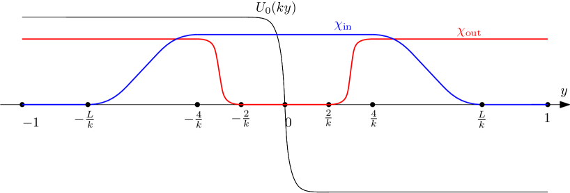
Figure 1. A sketch of the velocity profile $U(y)=U_{0}(ky)$ and the cutoffs $\chi_{{\rm in}}$, $\chi_{{\rm out}}$ leading to the multiscale estimate (14).

In order to introduce it, we let $L>1$ be a large number (to be specified) and we define the inner and outer cutoffs $\chi_{{\rm in}}$, $\chi_{{\rm out}}$ to be smooth functions such that $\chi_{{\rm in}}=1$ on $(-4/k,4/k)$, $\chi_{{\rm in}}=0$ outside $(-L/k,L/k)$, $\chi_{{\rm out}}=0$ in $(-2/k,2/k)$ and $\chi_{{\rm out}}=1$ outside $(-4/k,4/k)$ and

$$\chi_{{\rm in}}^{(l)}\leq\left(\frac{10k}{L}\right)^{l},\qquad\chi_{{\rm out}}^{(l)}\leq\left({10k}\right)^{l}\qquad\text{ for l=0,1,2, }$$ (11)

Note that $\chi_{{\rm in}}$ and $\chi_{{\rm out}}$ overlap, see Figure 1. We also define the inner function space

$$Y:=H^{1}(\mathbb{R}),$$ (12)

and the outer function space

$$Z:=H^{1}_{0}((-1,1)),\qquad\|f\|_{Z}:=\sqrt{\frac{L}{k}}\|f^{\prime}\|_{L^{2}}+\sqrt{kL}\|f\|_{L^{2}}.$$ (13)

Theorem 2.

There exists $L>1$ and $\varepsilon_{0},c_{0}>0$ with the following property: for all sufficiently large $k$ and all $\varepsilon\in(0,\varepsilon_{0}k^{2})$ there exist $c=c(\varepsilon,k)\in\mathbb{C}$ with $\mathrm{Im}\,c\sim\varepsilon/k^{2}>0$ and such that the Rayleigh equation (5) has a nontrivial solution $\phi\in H^{1}_{0}(-1,1)$, which admits the multiscale decomposition

$$\phi(y)=\phi_{{\rm out}}(y)\chi_{{\rm out}}(y)+\left(\Phi_{0}(ky)+\Psi(ky)\right)\chi_{{\rm in}}(y),$$

where $\Psi\in H^{1}$, $\phi_{{\rm out}}\in Z$ satisfy the estimates

$$\|\Psi\|_{H^{1}}+\|\phi_{{\rm out}}\|_{Z}\lesssim\varepsilon+\left|\frac{\widetilde{\alpha}^{2}}{k^{2}}-\alpha_{0}^{2}\right|+|c|+L^{-1/2}.$$ (14)

We present the proof of Theorem 2 in Section 1 below. The proof, including the gluing procedure described above and some estimates of the inner and outer equations, is inspired by the recent paper [4], which develops a multiscale approach for capturing instabilities of the 3D inviscid vortex columns. We also note a related result [2] on gluing nonunique solutions to the forced Navier-Stokes equations.

We emphasize that Theorem 2 is the first result that provides a link between the construction of linear instability for shear flows with the Kelvin-Helmholtz instability [5, 1, 15] of vortex sheets. For example, it is well-known in the context of the Kelvin-Helmholtz instability that considering independent modes of oscillations of a form similar to (1), the growth rate in time is predicted to be of the size proportional to $\alpha$, representing mode frequency in $x$ (see [5, (4.27)], for example). This is consistent with the scaling of Theorem 2, size the growth rate in time is $\alpha\mathrm{Im}\,c$ (recall (1)), and the maximal value of $\mathrm{Im}\,c$ is proportional to $\varepsilon_{0}=O(1)$.

We note that we do not claim any convergence result as $k\to\infty$. In fact, the relation of this limit with the problem of instabilities of vortex sheets remains an interesting open problem.

2. Proof of Theorem 1

Here we prove Theorem 1. We first let $K\colon L^{2}\to H^{1}_{0}\cap H^{2}$ denote the solution operator of

$$-\psi^{\prime\prime}+\widetilde{\alpha}^{2}\psi=f$$

with homogeneous Dirichlet boundary conditions at $y=\pm 1$. We note that $K$ is a compact operator from $L^{2}$ to $H^{s}$ for any $s\in[0,2)$. Taking $K$ of (8) we obtain

$$\psi+K\left(\frac{U^{\prime\prime}}{U}\psi+P\psi\right)=K\left(\varepsilon\phi+\left(\frac{U^{\prime\prime}}{U}-\frac{U^{\prime\prime}}{U-c}\right)\phi\right)$$ (15)

Denoting the left-hand side by $T\psi$ and the right-hand side by $R_{\varepsilon,c}$ we obtain

$$T\psi=R_{\varepsilon,c}\psi+R_{\varepsilon,c}\widetilde{\phi}.$$ (16)

In order to solve this equation for all small $\varepsilon,c>0$, we first show some properties of $T$ and $R_{\varepsilon,c}$.

Lemma 3.

$T\colon H^{1}_{0}\to H^{1}_{0}$ is invertible.

Proof.

We first note that, since $\phi\mapsto K\left(\frac{U^{\prime\prime}}{U}\phi+P\phi\right)$ is a compact operator $H^{1}_{0}\to H^{1}_{0}$, we have that $T$ is Fredholm of index $0$, and so it suffices to show that $\mathrm{ker}\,T=0$. To this end, suppose that $T\phi=0$, that is

$$L\phi+P\phi:=-\phi^{\prime\prime}+\widetilde{\alpha}^{2}\phi+\frac{U^{\prime\prime}}{U}\phi+P\phi=0$$ (17)

for some $\phi\in H^{1}_{0}$. Note that $L$ is self-adjoint, and that $L\phi=0$ if and only if $\phi\in\mathrm{Span}\,\{\widetilde{\phi}\}$. Multiplying (17) by $\widetilde{\phi}$ and integrating, we obtain

$$(P\phi,\widetilde{\phi})=-(L\phi,\widetilde{\phi})=-(\phi,L\widetilde{\phi})=0,$$

and so $P\phi\perp\widetilde{\phi}$. Thus $\phi=0$, as required. ∎

As for $R_{\varepsilon,c}$ we first consider the term $1/(U-c)$. We note that, since $a\in(-1,1)$ is an inflection point of $U$, we have $U^{\prime}(a)\neq 0$. Hence, for every sufficiently small $|c|$, there exists $a^{\prime}\in(-1,1)$ such that $U(a^{\prime})=c_{R}$, where $c=c_{R}+ic_{I}$. In the next lemma we show that $1/(U-c)$ can be approximated by a term resembling the Plemenj-Sokhotski formula (7).

Lemma 4 (Approximation lemma).

For sufficiently small $|c|$ we have that

$$\frac{1}{U(y)-c}-\frac{1}{U^{\prime}(a^{\prime})(y-a^{\prime})-ic_{I}}=O(1)+io(1)$$ (18)

uniformly for $y\in(-1,1)$, as $|c|\to 0$.

Proof.

We note that

$$\frac{1}{U(y)-c}-\frac{1}{U^{\prime}(a^{\prime})(y-a^{\prime})-ic_{I}}=\frac{U^{\prime\prime}(\xi)(y-a^{\prime})^{2}/2}{(U(y)-c)(U^{\prime}(a^{\prime})(y-a^{\prime})-ic_{I})},$$

and so

$$\left|\frac{1}{U(y)-c}-\frac{1}{U^{\prime}(a^{\prime})(y-a^{\prime})-ic_{I}}\right|\lesssim\frac{\|U^{\prime\prime}\|_{L^{\infty}(a-\delta,a+\delta)}|y-a^{\prime}|}{|U(y)-c_{R}|\inf_{(a-\delta,a+\delta)}|U^{\prime}|}\lesssim 1$$ (19)

for $|y-a^{\prime}|\leq\delta/2$ whenever $a^{\prime}\in[a-\delta/2,a+\delta/2]$, where $\delta>0$ is sufficiently small so that $U$ is strictly monotone in $(a-\delta,a+\delta)$. On the other hand, the same upper bound (dependent on $\delta$) is trivial in the case $|y-a^{\prime}|>\delta/2$.

As for the $o(1)$ part in (18), given $\varepsilon>0$ we take $\delta>0$ sufficiently small so that

$$\frac{1}{2}|U^{\prime}(a)|\leq|U^{\prime}(y)|\leq 2|U^{\prime}(a)|$$

for $y\in(a-\delta,a+\delta)$ and we let $\eta>0$ be such that

$$\|U^{\prime\prime}\|_{L^{\infty}(a-\eta,a+\eta)}\leq\frac{\varepsilon}{4|U^{\prime}(a)|^{2}}.$$

Then taking $|c|$ sufficiently small so that $a^{\prime}\in(a-\eta/2,a+\eta/2)$ we see from (19) that

$$\left|\frac{1}{U(y)-c}-\frac{1}{U^{\prime}(a^{\prime})(y-a^{\prime})-ic_{I}}\right|\lesssim\frac{4\|U^{\prime\prime}\|_{L^{\infty}(a-\eta,a+\eta)}}{|U^{\prime}(a)|^{2}}\leq\varepsilon$$

for $|y-a|\leq\eta/2$. For $|y-a|>\eta/2$ we take $|c|$ sufficiently small so that

$$\begin{split}&\left|\mathrm{Im}\left(\frac{1}{U(y)-c}-\frac{1}{U^{\prime}(a^{\prime})(y-a^{\prime})-ic_{I}}\right)\right|\\ &=\left|\frac{c_{I}\left(U^{\prime}(a^{\prime})(y-a^{\prime})+U(y)-c_{R}\right)U^{\prime\prime}(\xi)(y-a^{\prime})^{2}/2}{((U(y)-c_{R})U^{\prime}(a^{\prime})(y-a^{\prime})-c_{I}^{2})^{2}+(c_{I}(U^{\prime}(a^{\prime})(y-a^{\prime})+(U(y)-c_{R})c_{I})^{2}}\right|\\ &\lesssim_{\eta}|c_{I}|\frac{|U^{\prime\prime}(\xi)|(y-a^{\prime})^{2}}{U^{\prime}(a^{\prime})^{2}(y-a^{\prime})^{2}+O(|c|)}\lesssim_{\eta}|c_{I}|\leq\varepsilon,\end{split}$$

as required. ∎

We can use Lemma 4 to obtain logarithmic decay of the Fourier Sine coefficients of $1/(U-c)$.

Lemma 5.

If $|c|$ is sufficiently small then

$$\left|\int_{-1}^{1}\frac{1}{U(y)-c}\sin\frac{k\pi(y+1)}{2}\mathrm{d}y\right|\lesssim\log(1+k)$$ (20)

Proof.

Thanks to Lemma 4 it suffices to show that

$$\left|\int_{-1}^{1}\frac{1}{U^{\prime}(a^{\prime})(y-a^{\prime})-ic_{I}}\sin\frac{k\pi(y+1)}{2}\mathrm{d}y\right|\lesssim\log(1+k)$$ (21)

We have

$$\frac{1}{U^{\prime}(a^{\prime})(y-a^{\prime})-ic_{I}}=\frac{U^{\prime}(a^{\prime})(y-a^{\prime})+ic_{I}}{U^{\prime}(a^{\prime})^{2}(y-a^{\prime})^{2}+c_{I}^{2}}.$$

For the imaginary part, we obtain

$$\begin{split}\left|\int_{-1}^{1}\frac{c_{I}}{U^{\prime}(a^{\prime})^{2}(y-a^{\prime})^{2}+c_{I}^{2}}\sin\frac{k\pi(y+1)}{2}\,\mathrm{d}y\right|&\leq\int_{-1}^{1}\frac{|c_{I}|^{-1}}{(U^{\prime}(a^{\prime})(y-a^{\prime})/c_{I})^{2}+1}\mathrm{d}y\\ &\leq\frac{1}{|U^{\prime}(a^{\prime})|^{2}}\int_{\mathbb{R}}\frac{1}{z^{2}+1}\mathrm{d}z\lesssim 1.\end{split}$$

As for the real part, we expand $\sin(k\pi(y+1)/2)$ into a Taylor expansion at $a^{\prime}$ to obtain

$$\begin{split}\left|\int_{[-1,1]\cap\{|y-a^{\prime}|\leq 2/k}\frac{U^{\prime}(a^{\prime})(y-a^{\prime})}{U^{\prime}(a^{\prime})^{2}(y-a^{\prime})^{2}+c_{I}^{2}}\sin\,\frac{k\pi(y+1)}{2}\mathrm{d}y\right|&\lesssim k\int_{a^{\prime}-2/k}^{a^{\prime}+2/k}\frac{|U^{\prime}(a^{\prime})|(y-a^{\prime})^{2}}{U^{\prime}(a^{\prime})^{2}(y-a^{\prime})^{2}+c_{I}^{2}}\mathrm{d}y\\ &\lesssim k\int_{-2/k}^{2/k}\frac{y^{2}}{y^{2}+c_{I}^{2}}\mathrm{d}y\lesssim 1.\end{split}$$

For $|y-a^{\prime}|\geq 2/k$ we have that

$$\left|\int_{[-1,1]\cap\{|y-a^{\prime}|\geq 2/k\}}\frac{U^{\prime}(a^{\prime})(y-a^{\prime})}{U^{\prime}(a^{\prime})^{2}(y-a^{\prime})^{2}+c_{I}^{2}}\sin\,\frac{k\pi(y+1)}{2}\mathrm{d}y\right|\leq\frac{2}{|U^{\prime}(a^{\prime})|}\int_{2/k}^{2}\frac{1}{z}\mathrm{d}z\lesssim\log(1+k),$$

as required. ∎

Thanks to the above lemmas we can now establish

Lemma 6 (Remainder norm).

For every $c\in\mathbb{C}$, $\varepsilon>0$, $\|R_{\varepsilon,c}\|_{H^{1}_{0}\to H^{1}_{0}}\lesssim(|c|+|\varepsilon|)$.

Proof.

Letting $f:=(U-c)^{-1}$, and $g:=cU^{\prime\prime}\phi/U$ we see that

$$R_{\varepsilon,c}\phi=Kfg-\varepsilon\phi.$$

The first term on the right-hand side is the solution $\psi$ to $\psi^{\prime\prime}-\widetilde{\alpha}^{2}\psi=fg$, which we can estimate in $H^{1}$ by denoting by $h_{m}$ the $m$-th Fourier Sine coefficient of a function $h\colon(-1,1)\to\mathbb{C}$, and applying the Plancherel theorem,

$$\begin{split}\|\psi\|_{H^{1}}^{2}&\sim\sum_{k\in\mathbb{Z}}\frac{1+k^{2}}{(\widetilde{\alpha}^{2}+k^{2})^{2}}\left(\sum_{m\in\mathbb{Z}}g_{m}\log(1+|k-m|)\right)^{2}\\ &\lesssim\sum_{k\in\mathbb{Z}}\frac{1+k^{2}}{(\widetilde{\alpha}^{2}+k^{2})^{2}}\left(\sum_{m\in\mathbb{Z}}g_{m}(1+|k|)^{1/4}(1+|m|)^{1/4}\right)^{2}\\ &\lesssim\sum_{k\in\mathbb{Z}}\frac{(1+k^{2})(1+|k|)^{1/2}}{(\widetilde{\alpha}^{2}+k^{2})^{2}}\left(\sum_{m\in\mathbb{Z}}m^{3/2}|g_{m}|^{2}(1+|m|)^{1/2}\right)\left(\sum_{m\in\mathbb{Z}}\frac{1}{1+|m|^{3/2}}\right)\\ &\lesssim\|g\|_{H^{1}}^{2}\sum_{k\in\mathbb{Z}}\frac{(1+k^{2})(1+|k|)^{1/2}}{(\widetilde{\alpha}^{2}+k^{2})^{2}}\\ &\lesssim\|g\|_{H^{1}}^{2}\lesssim_{U}|c|^{2}\|\phi\|_{H^{1}}^{2},\end{split}$$

which gives the required estimate, where we used Lemma 5 in the first line. ∎

Remark 1.

We note that the above proof is the only place where we use the assumption that $U\in C^{5}$ (which is needed for the last inequality). This regularity is not essential; for example Lin [12] used only $C^{2}$ regularity, although one needs a little bit more (such as $U\in C^{2,\gamma}$ for some $\gamma>0$) in order to make sense of the principal value in Sokhotski-Plemenj formula (7). For such regularity an alternative proof of Lemma 6 below is needed, perhaps requiring $C^{\gamma}$ estimates, as in [3, Lemma 4.8.1], for example.

The invertibility of $T$ and the estimate on $\|R_{\varepsilon,c}\|$ let us rewrite the projected equation (8) as

$$\psi=T^{-1}\circ R_{\varepsilon,c}\psi+T^{-1}\circ R_{\varepsilon,c}\widetilde{\phi},$$

which has a unique solution $\psi$ for every sufficiently small $\varepsilon,|c|$, given by the Neumann series expansion,

$$\psi=(I-T^{-1}\circ R_{\varepsilon,c})^{-1}T^{-1}\circ R_{\varepsilon,c}\widetilde{\phi}=\sum_{k\geq 1}(T^{-1}\circ R_{\varepsilon,c})^{k}\widetilde{\phi}.$$ (22)

It thus remains to determine the choice of $\epsilon$, $c$ solving the reduced equation (9), namely the equation

$$G(c,\varepsilon)=0,$$ (23)

where we denoted by $\psi$ the solution (22) of the projected equation (8) for given $\epsilon$, $c$, and we set

$$G(c,\varepsilon):=(\psi,\widetilde{\phi})=(T^{-1}\circ R_{\varepsilon,c}\widetilde{\phi},\widetilde{\phi})+\sum_{k\geq 2}((T^{-1}\circ R_{\varepsilon,c})^{k}\widetilde{\phi},\widetilde{\phi}).$$ (24)

We have the following.

Lemma 7 (Expansion of $G$).

$G$ is holomorphic in $c\in\{z\in\mathbb{C}\colon\mathrm{Im}\,z>0\}$ and satisfies

$$G(c,\varepsilon)=c\lambda+\varepsilon+o(|c|+|\varepsilon|)$$ (25)

as $|c|,\varepsilon\to 0$, $\mathrm{Im}\,c>0$. where $\lambda\in\mathbb{C}$ has positive imaginary part.

Proof.

We first note that the last sum in (24) can be bounded by $o(|c|+\varepsilon)$,

$$\begin{split}\left|\sum_{k\geq 2}\left((T^{-1}\circ R_{\varepsilon,c})^{k}\widetilde{\phi},\widetilde{\phi}\right)\right|&\leq\sum_{k\geq 2}\|(T^{-1}\circ R_{\varepsilon,c})^{k}\|_{H^{1}_{0}\to H^{1}_{0}}\lesssim\sum_{k\geq 2}\|T^{-1}\|^{k}\|R_{\varepsilon,c}\|^{k}\\ &\lesssim\sum_{k\geq 2}(C(|\varepsilon|+|c|))^{k}\lesssim O((|\varepsilon|+|c|)^{2}).\end{split}$$

As for the linear term, we have

$$\left(T^{-1}\circ R_{\varepsilon,c}\widetilde{\phi},\widetilde{\phi}\right) =\left(T^{-1}\circ K\left(\frac{U^{\prime\prime}}{U}-\frac{U^{\prime\prime}}{U-c}\right)\widetilde{\phi},\widetilde{\phi}\right)+\varepsilon\left(T^{-1}\circ K\widetilde{\phi},\widetilde{\phi}\right)$$

$$=\left(\left(\frac{U^{\prime\prime}}{U}-\frac{U^{\prime\prime}}{U-c}\right)\widetilde{\phi},T^{-1}\circ K\widetilde{\phi}\right)+\varepsilon$$

$$=c\Gamma(c)+\varepsilon,$$

where we used the fact that $T\widetilde{\phi}=K\widetilde{\phi}$ (recall (15)), the fact that $T^{-1}\circ K$ is self-adjoint, and we set

$$\Gamma(c):=\left(\frac{-U^{\prime\prime}}{(U-c)U}\widetilde{\phi},\widetilde{\phi}\right).$$

It remains to show that

$$\lim_{c_{I}>0,c\to 0}\Gamma(c)=\lambda,$$

where $\lambda$ is a complex number with positive imaginary part.

Letting

$$h:=-\frac{U^{\prime\prime}}{U}|\widetilde{\phi}|^{2},$$

we see that $h$ is Hölder continuous on $[-1,1]$, and that

$$\Gamma(c)=\int_{-1}^{1}\frac{1}{(U-c)}h\,\mathrm{d}y= \int_{-1}^{1}\frac{1}{(U^{\prime}(a^{\prime})(y-a^{\prime})-ic_{I})}h(y)\,\mathrm{d}y$$

$$\hskip 56.9055pt+\int_{-1}^{1}\left(\frac{1}{U(y)-c}-\frac{1}{U^{\prime}(a^{\prime})(y-a^{\prime})-ic_{I}}\right)h(y)\,\mathrm{d}y$$

We now note that the last integrand in bounded, with its imaginary part converging pointwise to $0$, due to Lemma 4, and so applying the Dominated Convergence Theorem and the Plemenj-Sokhotski formula (7) (see also Lemma 8 for more details), we obtain that there exists $C\in\mathbb{R}$ such that

$$\Gamma(c)\to C+i\pi|U^{\prime}(a)|^{-1}h(a):=\lambda$$

as $c\to 0$, $\mathrm{Im}\,c>0$. Note that $\mathrm{Im}\,\lambda>0$, as required, since $U^{\prime}(a)\neq 0$ (recall the comments above Lemma 4), and $h(a)>0$ (recall assumption mentioned around (3) and (4)). ∎

With the expansion given by Lemma 7 we first note that, if there was no “$o(|c|+\varepsilon)$” in (25), then the only solution $c=\widetilde{c}(\varepsilon)$ to the reduced equation (23) would be

$$\widetilde{c}(\varepsilon):=\frac{-\varepsilon}{\lambda}=\frac{-\varepsilon\lambda_{R}+i\varepsilon\lambda_{I}}{|\lambda|^{2}},$$ (26)

which describes a straight line originating from $c=0$ (at $\varepsilon=0$) and propagating into the upper complex plane (so that $\mathrm{Im}\,c>0$ as required) as $\varepsilon$ increases. In order to incorporate the “$o(|c|+\varepsilon)$” term, we write

$$G(c,\varepsilon)=\underbrace{\lambda(a)(c-\widetilde{c})}_{=:f(c)}+\underbrace{o(\varepsilon+|c-\widetilde{c}|)}_{=:g(c)},$$

and we take $|c|,\varepsilon$ sufficiently small so that

$$|g(c,\varepsilon)|\leq\frac{\varepsilon}{8}+\frac{|\lambda(c-\widetilde{c}(\varepsilon))|}{4}.$$

Then, for such $\varepsilon$,

$$|g(\cdot,\varepsilon)|\leq\frac{2|\lambda(c-\widetilde{c}(\varepsilon))|}{8}+\frac{|f|}{4}=\frac{|f|}{2}<|f|\qquad\text{ on }\partial D\left(\widetilde{c}(\varepsilon),\frac{\varepsilon}{2|\lambda|}\right).$$

Thus, since, in $D\left(\widetilde{c}(\varepsilon),{\varepsilon}/{2|\lambda|}\right)$, both $g(\cdot,\varepsilon)$ and $f$ are holomorphic and $f$ has exactly one zero $\widetilde{c}(\varepsilon)$, Rouché Theorem implies that $G(\cdot,\varepsilon)=f+g(\cdot,\varepsilon)$ also has a unique zero in $D\left(\widetilde{c}(\varepsilon),{\varepsilon}/{2|\lambda|}\right)$, which gives the desired solution of the reduced equation (23).

3. Proof of Theorem 2

Here we prove Theorem 2. We let $\phi=\phi_{{\rm in}}\chi_{{\rm in}}+\phi_{{\rm out}}\chi_{{\rm out}}$. Then $\phi$ solves (5) if $\phi_{{\rm in}}$, $\phi_{{\rm out}}$ solve

$$\phi_{{\rm in}}^{\prime\prime}-\widetilde{\alpha}^{2}\phi_{{\rm in}}+\varepsilon\phi_{in}+\frac{U^{\prime\prime}}{U-c}\phi_{{\rm in}}=-2\phi_{{\rm out}}^{\prime}\chi_{{\rm out}}^{\prime}-\phi_{{\rm out}}\chi_{{\rm out}}^{\prime\prime},$$ (27)

$$\phi_{{\rm out}}^{\prime\prime}-\widetilde{\alpha}^{2}\phi_{{\rm out}}+\varepsilon\phi_{{\rm out}}=-2\phi_{{\rm in}}^{\prime}\chi_{{\rm in}}^{\prime}-\phi_{{\rm in}}\chi_{{\rm in}}^{\prime\prime}.$$ (28)

Let us apply the rescaling $R\colon L^{2}\to L^{2}$, $\Phi(\xi)=R\phi(\xi)=\phi(y)$, where $\xi:=ky$. Note that

$$\|R\|=k^{1/2},$$ (29)

and that $\widetilde{\alpha}/k-\alpha_{0}\to 0$ as $k\to\infty$ (see Lemma 9). We can thus rewrite (27) as the projection of the rescaled inner equation,

$$\begin{split}-\Psi^{\prime\prime}&+\alpha_{0}^{2}\Psi-\frac{U^{\prime\prime}}{U}\Psi+P_{0}\Psi=\frac{1}{k^{2}}R\left(2\phi_{{\rm out}}^{\prime}\chi_{{\rm out}}^{\prime}+\phi_{{\rm out}}\chi_{{\rm out}}^{\prime\prime}\right)\\ &\hskip 113.81102pt+\left(\frac{\varepsilon}{k^{2}}-\left(\frac{\widetilde{\alpha}^{2}}{k^{2}}-\alpha_{0}^{2}\right)+\left(\frac{U^{\prime\prime}}{U}-\frac{U^{\prime\prime}}{U-c}\right)\right)(\Psi+\Phi_{0})\end{split}$$ (30)

together with the reduced equation

$$(\Psi,\Phi_{0})=0,$$ (31)

where we used the decomposition

$$\Phi_{{\rm in}}=\Phi_{0}+\Psi,$$

and $P_{0}\Psi:=(\Psi,\Phi_{0})\Phi_{0}$ is the projection onto the neutral eigenfunction $\Phi_{0}$ of the inner problem (recall (10)).

As in Section 2 we let $K:L^{2}\to H^{2}$ denote the solution operator of $-\Psi^{\prime\prime}+\alpha_{0}^{2}\Psi=F$, namely

$$KF(\xi):=\frac{1}{2\alpha_{0}}\int_{\mathbb{R}}\mathrm{e}^{-\alpha_{0}|\xi-\eta|}F(\eta)\mathrm{d}\eta,$$

and we set

$$T\Psi:=\Psi+K\left(-\frac{U^{\prime\prime}}{U}\Psi+P_{0}\Psi\right),$$

and

$$R_{\delta,c}\Psi:=\left(\delta+\left(\frac{U^{\prime\prime}}{U}-\frac{U^{\prime\prime}}{U-c}\right)\right)\Psi$$

We observe, as in Lemma 3, that $T\colon H^{1}\to H^{1}$ is invertible and that

$$\|R_{\delta,c}\|_{H^{1}\to H^{1}}\lesssim\delta+|c|.$$

Thus, we can rewrite the projected inner equation (30) as

$$\Psi=T^{-1}\circ R_{\delta,c}(\Psi+\Phi_{0})+\underbrace{\frac{1}{k^{2}}T^{-1}\circ K\circ R\left(-2\phi_{{\rm out}}^{\prime}\chi_{{\rm out}}^{\prime}-\phi_{{\rm out}}\chi_{{\rm out}}^{\prime\prime}\right)}_{=:B\phi_{{\rm out}}},$$ (32)

where $\delta:=\frac{\varepsilon}{k^{2}}-\left(\frac{\widetilde{\alpha}^{2}}{k^{2}}-\alpha_{0}^{2}\right)$. We note that $\|B\|_{Z\to H^{1}}\lesssim L^{-1/2}$, since

$$\left\|R\left(2\phi_{{\rm out}}^{\prime}\chi_{{\rm out}}^{\prime}+\phi_{{\rm out}}\chi_{{\rm out}}^{\prime\prime}\right)\right\|\lesssim k^{1/2}\left(k\|\phi_{{\rm out}}^{\prime}\|+k^{2}\|\phi_{{\rm out}}\|\right)=\frac{k^{2}}{\sqrt{L}}\|\phi_{{\rm out}}\|_{Z},$$

where we used (29). Letting

$$\mathsf{C}\colon H^{1}\to Z,\quad\mathsf{C}\Upsilon=g\Leftrightarrow-g^{\prime\prime}+\widetilde{\alpha}^{2}g-\varepsilon g=2(R^{-1}\Upsilon)^{\prime}\chi_{{\rm in}}^{\prime}+R^{-1}\Upsilon\chi_{{\rm in}}^{\prime\prime}$$

for $\varepsilon<\widetilde{\alpha}^{2}/2$, one obtains

$$k\|(\mathsf{C}\Upsilon)^{\prime}\|+k^{2}\|\mathsf{C}\Upsilon\|\leq\left\|2(R^{-1}\Upsilon)^{\prime}\chi_{{\rm in}}^{\prime}+R^{-1}\Upsilon\chi_{{\rm in}}^{\prime\prime}\right\|\lesssim k^{1/2}\|\Upsilon^{\prime}\|\frac{k}{L}+k^{-1/2}\|\Upsilon\|\frac{k^{2}}{L^{2}}\lesssim\frac{k^{3/2}}{L}\|\Upsilon\|_{H^{1}},$$

i.e. that $\|\mathsf{C}\|_{H^{1}\to Z}\lesssim L^{-1/2}$. Thus, setting $\mathsf{A}:=T^{-1}\circ R_{\delta,c}\colon H^{1}\to H^{1}$, we can rewrite (27)–(28) as

$$\begin{pmatrix}I&0\\ 0&I\end{pmatrix}\begin{pmatrix}\Psi\\ \phi_{{\rm out}}\end{pmatrix}+\begin{pmatrix}-\mathsf{A}&-\mathsf{B}\\ -\mathsf{C}&0\end{pmatrix}\begin{pmatrix}\Psi\\ \phi_{{\rm out}}\end{pmatrix}=\begin{pmatrix}\mathsf{A}\Phi_{0}\\ \mathsf{C}\Phi_{0}\end{pmatrix}\qquad\text{ in }H^{1}\times Z,$$ (33)

Since

$$\|\mathsf{A}\|\lesssim\frac{\varepsilon}{k^{2}}+\left|\frac{\widetilde{\alpha}^{2}}{k^{2}}-\alpha_{0}^{2}\right|+|c|,\qquad\|\mathsf{B}\|,\|\mathsf{C}\|\lesssim L^{-1/2},$$

the system (33) has a unique solution for all sufficiently small $|\varepsilon|$, $|c|$ and sufficiently large $k$, satisfying estimate (14). In order to solve the reduced equation (31), we set, analogously to Lemma 7,

$$G(\delta,c):=(\Psi,\Phi_{0}),$$

where $\Psi$ is the solution to (33) with $\delta=\frac{\varepsilon}{k^{2}}-\left|\frac{\widetilde{\alpha}^{2}}{k^{2}}-\alpha_{0}^{2}\right|$. As below Lemma 7 we conclude that for every sufficiently small $\delta$ (i.e. for sufficiently small $\epsilon$ and sufficiently large $k$) there exists $c=c(\delta)$ such that $G(\delta,c)=0$, which concludes the proof of Theorem 2.

Appendix A Plemenj-Sokhotski formula

Lemma 8.

Let $a$ and $b$ be constants such that $a<0<b$. Let $f\in C^{0,\alpha}[a,b]$ for some $\alpha\in(0,1)$. Then

$$\lim_{(\delta,\epsilon)\to(0,0^{+})}\int^{b}_{a}\frac{f(x)}{x+\delta\pm i\epsilon}\,\mathrm{d}x=\mp i\pi f(0)+\mathrm{p.v.}\int^{b}_{a}\frac{f(x)}{x}\,\mathrm{d}x.$$ (34)

Proof.

We first write

$$\int^{b}_{a}\frac{f(x)}{x+\delta+i\epsilon}\,\mathrm{d}x=\int^{b}_{a}\frac{f(x)(x+\delta)}{(x+\delta)^{2}+\epsilon^{2}}\,\mathrm{d}x-\int^{b}_{a}\frac{i\epsilon f(x)}{(x+\delta)^{2}+\epsilon^{2}}\,\mathrm{d}x.$$ (35)

Given $\gamma\in(0,1)$ we write the first integral on the right-hand side as

$$\int^{b}_{a}\frac{f(x)(x+\delta)}{(x+\delta)^{2}+\epsilon^{2}}\,\mathrm{d}x= \int_{(a,b)\setminus(-\gamma,\gamma)}\frac{f(x)(x+\delta)}{(x+\delta)^{2}+\epsilon^{2}}\,\mathrm{d}x+$$

$$+\int^{\gamma}_{-\gamma}\frac{(f(x)-f(-\delta))(x+\delta)}{(x+\delta)^{2}+\epsilon^{2}}\,\mathrm{d}x+f(-\delta)\int^{\gamma}_{-\gamma}\frac{(x+\delta)}{(x+\delta)^{2}+\epsilon^{2}}\,\mathrm{d}x.$$ (36)

For $|x|\geq\gamma$ and $|\delta|<\gamma/2$ we consider the first integral on the right-hand side by noting that

$$\left|\frac{f(x)(x+\delta)}{(x+\delta)^{2}+\epsilon^{2}}\right|,\left|\frac{f(x)}{(x+\delta)^{2}+\epsilon^{2}}\right|\lesssim\frac{|f(x)|}{|x+\delta|}+\frac{|f(x)|}{|x+\delta|^{2}}\lesssim\|f\|_{\infty}/\gamma^{2},$$ (37)

and so applying the Dominated Convergence Theorem, we obtain

$$\int_{(a,b)\setminus(-\gamma,\gamma)}\frac{f(x)(x+\delta)}{(x+\delta)^{2}+\epsilon^{2}}\,\mathrm{d}x\to\int_{(a,b)\setminus(-\gamma,\gamma)}\frac{f(x)}{x}\,\mathrm{d}x$$

as ${(\delta,\epsilon)\to(0,0^{+})}$. For the second term on the right-hand side of (A), we have

$$\left|\int^{\gamma}_{-\gamma}\frac{(f(x)-f(-\delta))(x+\delta)}{(x+\delta)^{2}+\epsilon^{2}}\,\mathrm{d}x\right|\lesssim\int^{\gamma}_{-\gamma}\frac{|x+\delta|^{1+\alpha}}{(x+\delta)^{2}+\epsilon^{2}}\,\mathrm{d}x\lesssim\int^{\gamma}_{-\gamma}{|x+\delta|^{\alpha-1}}\,\mathrm{d}x\lesssim_{\alpha}\gamma^{\alpha},$$ (38)

where we used the Hölder continuity assumption on $f$. Thus

$$\limsup_{(\delta,\epsilon)\to(0,0)}\left|\int^{\gamma}_{-\gamma}\frac{(f(x)-f(-\delta))(x+\delta)}{(x+\delta)^{2}+\epsilon^{2}}\,dx\right|\leq C_{\alpha}\gamma^{\alpha}.$$

For the last integral in (A), we have

$$\lim_{(\delta,\epsilon)\to(0,0^{+})}\int^{\gamma}_{-\gamma}\frac{f(-\delta)(x+\delta)}{(x+\delta)^{2}+\epsilon^{2}}\,\mathrm{d}x=\lim_{(\delta,\epsilon)\to(0,0^{+})}\frac{f(-\delta)}{2}\log\left(\frac{(\delta+\gamma)^{2}+\epsilon^{2}}{(\delta-\gamma)^{2}+\epsilon^{2}}\right)=0.$$

As for the imaginary part in (35) we write $\int^{b}_{a}=\int_{-\gamma}^{\gamma}+\int_{(a,b)\setminus(-\gamma,\gamma)}$. For the first of the resulting terms we use (37) and the Dominated Convergence Theorem to obtain that

$$\int_{(a,b)\setminus(-\gamma,\gamma)}\frac{\epsilon f(x)}{(x+\delta)^{2}+\epsilon^{2}}\,\mathrm{d}x\to 0$$

as $(\delta,\varepsilon)\to(0,0^{+})$. For the second one we see that

$$\left|\int^{\gamma}_{-\gamma}\frac{\epsilon(f(x)-f(-\delta))}{(x+\delta)^{2}+\epsilon^{2}}\,\mathrm{d}x\right|\lesssim\int^{\gamma}_{-\gamma}\frac{\epsilon|x+\delta|^{\alpha}}{(x+\delta)^{2}+\epsilon^{2}}\,\mathrm{d}x\lesssim\gamma^{\alpha},$$

and

$$f(-\delta)\int_{-\gamma}^{\gamma}\frac{\epsilon}{(x+\delta)^{2}+\epsilon}\mathrm{d}x=f(-\delta)\int_{(-\gamma+\delta)/\epsilon}^{(\gamma+\delta)/\epsilon}\frac{1}{1+z^{2}}\mathrm{d}z\to\pi f(0)\quad\text{ as }(\delta,c)\to(0,0^{+}).$$

Collecting all the terms, we obtain

$$\lim_{(\delta,\epsilon)\to(0,0^{+})}\int^{b}_{a}\frac{f(x)}{x+\delta+i\epsilon}\,\mathrm{d}x=-i\pi f(0)+\left(\int^{-\gamma}_{a}\frac{f(x)}{x}\,\mathrm{d}x+\int_{\gamma}^{b}\frac{f(x)}{x}\,\mathrm{d}x\right)+O(\gamma^{\alpha}).$$

Letting $\gamma\to 0$ completes the proof. ∎

Appendix B Eigenvalue problems

Here we consider the eigenvalue problem

$$-\Psi^{\prime\prime}+\beta^{2}\Psi+M(y)\Psi\qquad\text{ on }(-a,a),$$ (39)

equipped with homogeneous boundary conditions $\Psi(-a)=\Psi(a)=0$, where $M(y)$ is a nonpositive function with compact support in $\mathbb{R}$.

Lemma 9.

Let $\beta_{a}^{2}$ denote the largest eigenvalue of (39). Then $\beta_{a}^{2}\to\beta$ as $a\to\infty$, where $\beta$ is the maximal eigenvalue of (39) with $a=\infty$.

Proof.

See [19, Chapter II] ∎