Dark-state solution and hidden symmetries of the two-qubit multimode asymmetric quantum Rabi model

Abstract

We study the two-qubit asymmetric quantum Rabi model (AQRM) and find another hidden symmetry related to its dark-state solution. Such a solution has at most one photon and constant eigenenergy in the whole coupling regime, causing level crossings in the spectrum, although there is no explicit conserved quantity except energy, indicating another hidden symmetry. We find a symmetric operator in the eigenenergy basis to label the degeneracy with its eigenvalues, and compare it with the well-known hidden symmetry which exists when bias parameter $\epsilon$ is a multiple of half of the resonator frequency. Extended to the multimode case, we find not only hidden symmetries mentioned above, but also symmetries related with conserved bosonic number operators. This provides a new perspective for hidden symmetry studies on generalized Rabi models.

Keywords: asymmetric quantum Rabi model, hidden symmetry, dark state solution, Bogoliubov transformation

1 Introduction

The quantum Rabi model (QRM) [1] describes the interaction between a single-mode cavity and a qubit. It has wide applications in quantum optics [2, 3, 4, 5, 6, 7], circuit quantum electrodynamics (QED) [8, 9, 10, 11, 12], cavity QED [13, 14, 15, 16, 17, 18], quantum information [19, 20, 21] and so on [22, 23, 24]. Its semiclassical form was first introduced by Rabi [25, 26]. In 1963, Jaynes and Cummings [1] carried out the rotating wave approximation (RWA) [27] for the QRM under the conditions of near resonance and weak coupling, and obtained the analytical solution. However, the ultrastrong [28] and even deep strong coupling [29] has been realized in experiments, where the RWA fails. The analytical solution to the QRM was found by Braak [30] in 2011 in the Bargmann [31] space, and then retrieved by Chen et al with Bogoliubov operator approach [32]. There are many interesting studies on QRM and its generalizations [33, 34, 35, 36, 37, 38, 39, 40, 41, 42, 43, 44, 45, 46, 47] recently. Since there is no closed subspace in the photon number space, the eigenstate normally consists of infinite photons, making the dynamics in the ultrastrong coupling regime quite complex. However, there are special dark states with finite photons for the multiqubit and multimode case [48, 49, 50, 51], since the coherent superposition of basis with $N$-photon will cancel the population of higher photon number states when applied by the Hamiltonian. Such solutions exist in the whole qubit-photon coupling regime with constant eigenenergy when $N=1$. Taking advantage of such special dark states, one can fast generate $W$-states [51] and high-quality single photon sources [52] in the ultrastrong coupling regime deterministically through adiabatic evolution.

Meanwhile, the AQRM has attracted much interest recently. It has an additional static bias term $\epsilon\sigma_{x}$, which was considered physically as a spontaneous transition of the qubit [30]. Moreover, the AQRM widely appears in circuit QED systems, where the static bias of the superconducting flux qubit can be tuned externally [53, 56, 54, 55]. This provides more options for precise quantum control of the system. For the AQRM Hamiltonian, the presence of the static bias breaks the $\mathbbm{Z}_{2}$ symmetry $R=\exp{(i\pi a^{\dagger}a)}\sigma_{z}$ of the QRM. Hence, generally there is no level crossing in the spectrum. However, recent studies [30] have found that level crossings are restored when $\epsilon$ takes half-integer value of $\omega$, indicating a hidden symmetry in the AQRM [57, 58, 59]. In addition, many works [59, 60] have rigorously constructed the hidden symmetry operators using different methods, and inspired people to study the hidden symmetry of generalized AQRMs [61, 62, 63, 64].

Recent hidden symmetry studies of the ARQM focus on the case of $\epsilon$ is a multiple of $\omega/2$ [58, 59, 61, 60, 65]. However, it is interesting to explorer whether there are other kinds of hidden symmetries. In this paper, we first study the two-qubit AQRM and find a special dark state with at most one photon and constant eigenenergy in the whole coupling regime, corresponding to a horizontal line in the spectrum. Apparently, this horizontal line will bring in level crossings, indicating the existence of a hidden symmetry. However, this symmetry is different from the hidden symmetry mentioned above [61], because the level crossings here only happen between the one-photon solution and other energy levels. This symmetry brought about by the dark-state solution still exists even when $\epsilon=0$. We analyze this new level crossing and find another hidden symmetry with explicit expression given in the eigenenergy basis, and compare it with the hidden symmetry operator [61] when $\epsilon$ is a multiple of $\omega/2$. We extend AQRM to the $M$-mode case and introduce a Bogoliubov transformation [50] to rewrite the Hamiltonian, so that the dark state solution and hidden symmetry operator can be directly obtained. These two hidden symmetries still exist and are described explicitly. Moreover, there are other $M-1$ symmetries related with conserved bosonic number operator $b_{j}^{\dagger}b_{j}$ for $j=2,\ldots,M$.

The paper is structured as follows. In section 2, we study the two-qubit AQRM and find a special dark state. It corresponds to a horizontal line in the spectrum, indicating a hidden symmetry. We analyze this hidden symmetry and compare it with the case when $\epsilon$ is a multiple of $\omega/2$. In section 3, we extend our study to the multimode AQRM and find a series of new symmetries. A brief conclusion is given in section 4.

2 Special dark state solution and another hidden symmetry of the two-qubit AQRM

The Hamiltonian of the two-qubit AQRM reads ($\hbar$=1)

$$H=\omega a^{\dagger}a+g_{1}\sigma_{1x}(a^{\dagger}+a)+g_{2}\sigma_{2x}(a^{\dagger}+a)+\Delta_{1}\sigma_{1z}+\Delta_{2}\sigma_{2z}+\epsilon_{1}\sigma_{1x}+\epsilon_{2}\sigma_{2x},$$ (1)

where $a^{\dagger}$ and $a$ are creation and annihilation operators with cavity frequency $\omega$, respectively. The two qubits are described by Pauli matrices $\sigma_{x}$ and $\sigma_{z}$ with the energy level splitting $2\Delta$. $g_{1}$ and $g_{2}$ are the qubit–photon coupling constants for the two qubits, respectively. $\epsilon_{1}$ and $\epsilon_{2}$ are the static bias of the two qubits, respectively.

For this Hamiltonian, the presence of the static bias breaks the $\mathbbm{Z}_{2}$ symmetry $R=\exp(i\pi a^{\dagger}a)\sigma_{1z}\sigma_{2z}$. The eigenstates generally consist of infinite photon number states. However, finding certain special solution with finite photons will be interesting and useful [51, 52] for fast quantum information protocols using ultrastrong coupling. Supposing there is an eigenstate with at most one photon $|\psi\rangle=c_{0,1}|0,g,g\rangle+c_{0,2}|0,e,e\rangle+c_{0,3}|0,e,g\rangle+c_{0,4}|0,g,e\rangle+c_{1,1}|1,g,g\rangle+c_{1,2}|1,e,e\rangle+c_{1,3}|1,e,g\rangle+c_{1,4}|1,g,e\rangle$, then the eigenenergy equation reads ( $\omega$ is set to 1)

$$\begin{pmatrix}-\Delta_{1}-\Delta_{2}-E&0&\epsilon_{1}&\epsilon_{2}&0&0&g_{1}&g_{2}\\ 0&\Delta_{1}+\Delta_{2}-E&\epsilon_{2}&\epsilon_{1}&0&0&g_{2}&g_{1}\\ \epsilon_{1}&\epsilon_{2}&\Delta_{1}-\Delta_{2}-E&0&g_{1}&g_{2}&0&0\\ \epsilon_{2}&\epsilon_{1}&0&-\Delta_{1}+\Delta_{2}-E&g_{2}&g_{1}&0&0\\ 0&0&g_{1}&g_{2}&1-\Delta_{1}-\Delta_{2}-E&0&\epsilon_{1}&\epsilon_{2}\\ 0&0&g_{2}&g_{1}&0&1+\Delta_{1}+\Delta_{2}-E&\epsilon_{2}&\epsilon_{1}\\ g_{1}&g_{2}&0&0&\epsilon_{1}&\epsilon_{2}&1+\Delta_{1}-\Delta_{2}-E&0\\ g_{2}&g_{1}&0&0&\epsilon_{2}&\epsilon_{1}&0&1-\Delta_{1}+\Delta_{2}-E\\ 0&0&0&0&0&0&\sqrt{2}g_{1}&\sqrt{2}g_{2}\\ 0&0&0&0&0&0&\sqrt{2}g_{2}&\sqrt{2}g_{1}\\ 0&0&0&0&\sqrt{2}g_{1}&\sqrt{2}g_{2}&0&0\\ 0&0&0&0&\sqrt{2}g_{2}&\sqrt{2}g_{1}&0&0\\ \end{pmatrix}\begin{pmatrix}c_{0,1}\\ c_{0,2}\\ c_{0,3}\\ c_{0,4}\\ c_{1,1}\\ c_{1,2}\\ c_{1,3}\\ c_{1,4}\\ \end{pmatrix}=0,$$ (2)

which requires

$$\normalsize\left|\begin{array}[]{cccc}0&0&\sqrt{2}g_{1}&\sqrt{2}g_{2}\\ 0&0&\sqrt{2}g_{2}&\sqrt{2}g_{1}\\ \sqrt{2}g_{1}&\sqrt{2}g_{2}&0&0\\ \sqrt{2}g_{2}&\sqrt{2}g_{1}&0&0\\ \end{array}\right|=0\\ .$$ (3)

Such that $g_{2}=\pm g_{1}=g$, $c_{1,1}=\mp c_{1,2}$, $c_{1,3}=\mp c_{1,4}$, and equation (2) reduces to

$$\begin{pmatrix}-\Delta_{1}-\Delta_{2}-E&0&\epsilon_{1}&\epsilon_{2}&0&0\\ 0&\Delta_{1}+\Delta_{2}-E&\epsilon_{2}&\epsilon_{1}&0&0\\ \epsilon_{1}&\epsilon_{2}&\Delta_{1}-\Delta_{2}-E&0&0&0\\ \epsilon_{2}&\epsilon_{1}&0&-\Delta_{1}+\Delta_{2}-E&0&0\\ 0&0&\pm g&g&1-\Delta_{1}-\Delta_{2}-E&\epsilon_{1}\mp\epsilon_{2}\\ 0&0&g&\pm g&\mp(1+\Delta_{1}+\Delta_{2}-E)&\epsilon_{2}\mp\epsilon_{1}\\ \pm g&g&0&0&\epsilon_{1}\mp\epsilon_{2}&1+\Delta_{1}-\Delta_{2}-E\\ g&\pm g&0&0&\epsilon_{2}\mp\epsilon_{1}&\mp(1-\Delta_{1}+\Delta_{2}-E)\\ \end{pmatrix}\begin{pmatrix}c_{0,1}\\ c_{0,2}\\ c_{0,3}\\ c_{0,4}\\ c_{1,1}\\ c_{1,3}\\ \end{pmatrix}=0.$$ (4)

If there are less nonzero rows than columns in the above $8\times 6$ coefficient matrix after elementary row transformation, then there are nontrivial solutions. This can be done when $E=1$, $g_{2}=\pm g_{1}=g$, $\epsilon_{2}=\pm\epsilon_{1}=\epsilon$, $\epsilon^{2}=\dfrac{\Delta_{1}^{4}+(-1+\Delta_{2}^{2})^{2}-2\Delta_{1}^{2}(1+\Delta_{2}^{2})}{4}\geq 0$, and the coefficient matrix becomes

$$\small\begin{pmatrix}1&0&0&0&0&\dfrac{\mp(\Delta_{1}-\Delta_{2})(-1+\Delta_{1}+\Delta_{2})}{2g}\\ 0&1&0&0&0&\dfrac{(\Delta_{1}-\Delta_{2})(1+\Delta_{1}+\Delta_{2})}{2g}\\ 0&0&1&0&0&\dfrac{-\epsilon(\Delta_{1}-\Delta_{2})}{g(-1+\Delta_{1}-\Delta_{2})}\\ 0&0&0&1&0&\dfrac{\pm\epsilon(\Delta_{1}-\Delta_{2})}{g(1+\Delta_{1}-\Delta_{2})}\\ 0&0&0&0&1&\dfrac{\mp 2\epsilon(\Delta_{1}-\Delta_{2})}{(-1+\Delta_{1}-\Delta_{2})(\Delta_{1}+\Delta_{1}^{2}+\Delta_{2}-\Delta_{2}^{2})}\\ 0&0&0&0&0&0\\ 0&0&0&0&0&0\\ 0&0&0&0&0&0\\ \end{pmatrix}.$$ (5)

Therefore, the eigenstate reads

$$|\psi_{R{\epsilon}}\rangle= \frac{1}{{\cal N}}[\dfrac{\pm(\Delta_{1}-\Delta_{2})(-1+\Delta_{1}+\Delta_{2})}{2}|0,g,g\rangle-\dfrac{(\Delta_{1}-\Delta_{2})(1+\Delta_{1}+\Delta_{2})}{2}|0,e,e\rangle$$ (6)

$$+\dfrac{\epsilon(\Delta_{1}-\Delta_{2})}{-1+\Delta_{1}-\Delta_{2}}|0,e,g\rangle\mp\dfrac{\epsilon(\Delta_{1}-\Delta_{2})}{1+\Delta_{1}-\Delta_{2}}|0,g,e\rangle+g|1\rangle(|e,g\rangle\mp|g,e\rangle)$$

$$\pm\dfrac{2\epsilon(\Delta_{1}-\Delta_{2})}{(-1+\Delta_{1}-\Delta_{2})(\Delta_{1}+\Delta_{1}^{2}+\Delta_{2}-\Delta_{2}^{2})}g|1\rangle(|g,g\rangle\mp|e,e\rangle)].$$

Since it has constant energy and exists independent of the relation between $g$ and other parameters, it corresponds to a horizontal line in the spectrum, as shown in figure 1(a), while still being a qubit-photon entangled state. Obviously, this horizontal line will bring level crossings, although there is no explicit conserved quantity except energy. This indicates the existence of a hidden symmetry. Its prominent characteristic is that the level crossings only happens between $|\psi_{R{\epsilon}}\rangle$ and other energy levels, therefore we can label this degeneracy sufficiently with the eigenvalues of $|\psi_{R{\epsilon}}\rangle\langle\psi_{R{\epsilon}}|$, $0$ and $1$. This operator obviously commutes with $H$, and has an analytical form.

Actually, symmetric operators can be expressed in the eigenenergy basis as $\hat{S}=\sum_{i,j}s_{i}|\psi_{i,j}\rangle\langle\psi_{i,j}|$, where $\psi_{i,j}$ is the $j$-th eigenstate of $\hat{S}$ with eigenvalue $s_{i}$ [58]. We can obtain the information of $\hat{S}$ from the spectrum. If level crossings only happen between two groups of energy levels, then we only need two $s_{i}^{\prime}$s to label the degeneracy. If $s_{i}=\pm 1$, then $\hat{S}$ can be a parity operator, e.g., $\exp{(i\pi a^{\dagger}a)}\sigma_{z}=\sum_{n}(|\psi_{+,n}\rangle\langle\psi_{+,n}|-|\psi_{-,n}\rangle\langle\psi_{-,n}|)$ for the standard QRM. Or in some cases, $s_{i}$ is dependent on parameters, and then so does $\hat{S}$, e.g., the hidden symmetry operator $J$ obtained in [59, 60] for the AQRM. If level crossings happen between $N$ groups of energy levels, then $\hat{S}$ should have $N$ eigenvalues. E. g., for the standard Jaynes-Cumming model, the conserved excitation number operator $C=a^{\dagger}a+(\sigma_{z}+1)/2=\sum_{i=1,2,3\ldots}i(|\psi_{i,+}\rangle\langle\psi_{i,+}|+|\psi_{i,-}\rangle\langle\psi_{i,-}|)$ is obtained by choosing $s_{i}=0,1,2,3\ldots$. Here level crossings only happen between $|\psi_{R{\epsilon}}\rangle$ and other energy levels, so it is convenient to study its symmetric operator in the eigenenergy basis. We can easily write $\hat{S}=|\psi_{R{\epsilon}}\rangle\langle\psi_{R{\epsilon}}|+f(\Delta_{1,2},\epsilon,g)\sum_{\psi\neq\psi_{R{\epsilon}}}|\psi\rangle\langle\psi|$. The simplest choice is $f(\Delta_{1,2},\epsilon,g)=0$, where $\hat{S}$ can have an analytical form, which is still dependent on parameters. Whether it can be written in terms of $a$ and $a^{\dagger}$ still needs to be explored.

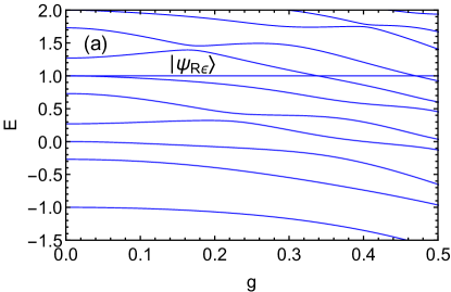
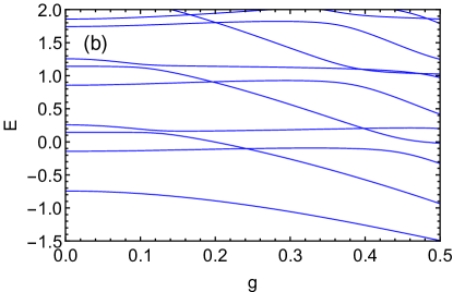
Figure 1: The spectrum of the two-qubit AQRM with (a) $\Delta_{1}=0.6$, $\Delta_{2}=0.3$, $\epsilon_{1}=\epsilon_{2}=\epsilon=\dfrac{\sqrt{1729}}{200}$, and (b) $g_{1}=g_{2}=g$, $\Delta_{1}=\Delta_{2}=0.8$, $\epsilon_{1}=1/2$, $\epsilon_{2}=0$.

As discussed in [61], there is another kind of level crossings in the two-qubit AQRM, where $\epsilon_{1}=1/2$, $\epsilon_{2}=0$, $g_{1}=g_{2}$, $\Delta_{1}=\Delta_{2}$, which is depicted in figure 1(b). This level crossings is brought about by the hidden symmetry operator [61], which reads

$$e^{i\pi a^{\dagger}a}\begin{pmatrix}a^{\dagger}-a+4g+\dfrac{\Delta}{g}&0&a^{\dagger}+a&0\\ 0&-a^{\dagger}+a-\dfrac{\Delta}{g}&-4g&-a^{\dagger}-a\\ -a^{\dagger}-a&-4g&-a^{\dagger}+a+\dfrac{\Delta}{g}&0\\ 0&a^{\dagger}+a&0&a^{\dagger}-a+4g-\dfrac{\Delta}{g}\\ \end{pmatrix}$$ (7)

in the qubit basis $\{|e,e\rangle,|e,g\rangle,|g,e\rangle,|g,g\rangle\}$. Different from the former case, here level crossings happen between different energy levels, so it is impossible to label all the degeneracies with a certain $|E_{n}\rangle\langle E_{n}|$. This operator is written in the qubit basis and contains $a$ and $a^{\dagger}$.

Actually, hidden symmetries of generalized Rabi models do not only exist in the above cases. There are hidden symmetries in the asymmetric N-qubit [61], two-mode [63], two-photon [62, 66], anisotropic and the Rabi–Stark model [64, 57]. These level crossings are all brought about by the qubit bias. However, they can also present even in the absence of the bias. Choosing $\epsilon=0$ in equation (6), $|\psi_{R\epsilon}\rangle$ reduces to

$$|\psi_{R}\rangle =\frac{1}{{\cal N}^{\prime}}[(\Delta_{2}-\Delta_{1})|0,e,e\rangle+g|1\rangle(|e,g\rangle\mp|g,e\rangle)],$$ (8)

with the condition $\Delta_{1}+\Delta_{2}=1$, $g_{2}=\pm g_{1}=g$, and $E=1$, which has been found in [67]. This solution still corresponds to a horizontal line in the spectrum and obviously cause level crossings in the parity subspace. So although the parity $\exp{(i\pi a^{\dagger}a)}\sigma_{1z}\sigma_{2z}$ is restored, we still need another conserved quantity (hidden symmetry) to label such level crossings within the same parity subspace. We can construct such operator by $\hat{S}=|\psi_{R}\rangle\langle\psi_{R}|+f(\Delta_{1,2},g)\sum_{\psi\neq\psi_{R}}|\psi\rangle\langle\psi|$ in the eigenenergy basis, because level crossings only happen between $|\psi_{R}\rangle$ and other energy levels. Such results shed new light on current hidden symmetry studies which focus on the qubit bias.

3 Extended to the multimode case

The multimode two-qubit AQRM reads

$$H_{M} = \sum_{i=1}^{M}\omega_{i}a_{i}^{\dagger}a_{i}+\Delta_{1}\sigma_{1z}+\Delta_{2}\sigma_{2z}+\sum_{i=1}^{M}g_{i1}\sigma_{1x}(a_{i}^{\dagger}+a_{i})$$ (9)

$$+\sum_{i=1}^{M}g_{i2}\sigma_{2x}(a_{i}^{\dagger}+a_{i})+\epsilon_{1}\sigma_{1x}+\epsilon_{2}\sigma_{2x},$$

where $a_{i}^{\dagger}$ and $a_{i}$ are the $i$-th photon mode creation and annihilation operators with frequency $\omega_{i}$, respectively. $g_{i1}$ and $g_{i2}$ are the qubit-photon coupling strength between the $i$-th mode and two qubits, respectively.

When $\omega_{i}=\omega$ and $g_{i1}/g_{i^{\prime}1}=g_{i2}/g_{i^{\prime}2}$, we can introduce similar Bogoliubov operators as proposed in [50]

$$b_{1} = \dfrac{\sum_{i=1}^{M}g_{i1}a_{i}}{\sqrt{\sum_{i=1}^{M}g_{i1}^{2}}},$$ (10)

$$b_{j} = \dfrac{\sum_{i=1}^{j-1}g_{i1}g_{j1}a_{i}-\sum_{i=1}^{j-1}g_{i1}^{2}a_{j}}{\sqrt{\sum_{i=1}^{j}g_{i1}^{2}\sum_{i=1}^{j-1}g_{i1}^{2}}},\ \ j=2,3,\dots,M$$ (11)

to transform equation (9) into

$$H_{M}^{\prime} = \omega b_{1}^{\dagger}b_{1}+\Delta_{1}\sigma_{1z}+\Delta_{2}\sigma_{2z}+\left[(\sum_{i=1}^{M}g_{i1}^{2})^{\frac{1}{2}}\sigma_{1x}+(\sum_{i=1}^{M}g_{i2}^{2})^{\frac{1}{2}}\sigma_{2x}\right](b_{1}^{\dagger}+b_{1})$$

$$+\epsilon_{1}\sigma_{1x}+\epsilon_{2}\sigma_{2x}+\omega\sum_{j=2}^{M}b_{j}^{\dagger}b_{j}.$$

$H_{M}^{\prime}$ is a combination of the two-qubit AQRM and $M-1$ free bosonic modes. So its solution takes the form of $|\psi_{b_{1}}\prod_{j=2}^{M}n_{b_{j}}\rangle$. $|n_{b_{j}}\rangle$ is the eigenstate of $b_{j}^{\dagger}b_{j}$ and $|\psi_{b_{1}}\rangle$ can be obtained from the solution of the single mode case by replacing $g_{1}$ with $(\sum_{i=1}^{M}g_{i1})^{\frac{1}{2}}$, $g_{2}$ with $(\sum_{i=1}^{M}g_{i2})^{\frac{1}{2}}$ and $a$ by $b_{1}$. Dark-state solution to the two-qubit AQRM $|\psi_{R{\epsilon}}\rangle$ exists when $g_{1}=g_{2}=g$, so a similar solution $|\psi_{R{\epsilon}}^{\prime}\rangle$ for the multimode case also requires $(\sum_{i=1}^{M}g_{i1})^{\frac{1}{2}}=(\sum_{i=1}^{M}g_{i2})^{\frac{1}{2}}=g_{b}$. Considering $g_{i1}/g_{i^{\prime}1}=g_{i2}/g_{i^{\prime}2}$, we arrive at $g_{i1}=g_{i2}=g^{\prime}_{i}$, and $|\psi_{R{\epsilon}}^{\prime}\rangle$ can be obtained by replacing $|1\rangle=a^{\dagger}|0\rangle$ with $|W_{M}\rangle=b_{1}^{\dagger}|0\rangle=(\sum_{i=1}^{M}{g^{\prime}_{i}}^{2})^{-\frac{1}{2}}\sum_{i=1}^{M}g_{i}^{\prime}|0_{1}0_{2}\dots 1_{i}0_{i+1}\dots 0_{M}\rangle$, and $g$ with $g_{b}$ in $|\psi_{R{\epsilon}}\rangle$ (equation (6)), and choosing $n_{b_{j}}=0$, as shown in figure 2 (a). Such a horizontal line will obviously cause level crossings. Its degeneracy can be labelled by the eigenvalues of $|\psi_{R{\epsilon}}^{\prime}\rangle\langle\psi_{R{\epsilon}}^{\prime}|$, $0$ and $1$. Meanwhile, the dashed lines with $n_{b_{j}}\neq 0$ are translations of the same-color solid lines with $n_{b_{j}}=0$ by $n_{b_{j}}\omega$, which will cause another kind of level crossings between energy levels with different $n_{b_{j}}$, as found in the multimode QRM without bias [50]. The corresponding symmetry operator reads $b^{\dagger}_{j}b_{j}$, and can be used to label the degeneracies by its eigenvalues $n_{b_{j}}=0,1,2,\ldots$.

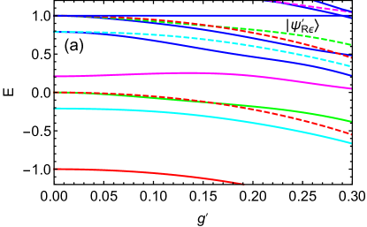
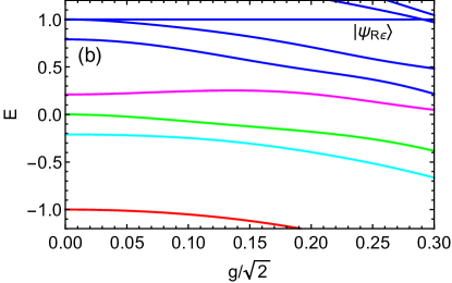
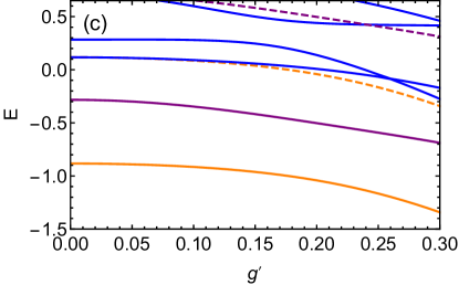
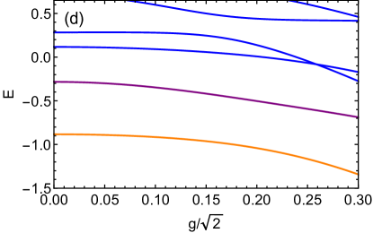
Figure 2: (a) and (c) Spectrum of the two-qubit two-mode AQRM with $\omega_{1}=\omega_{2}=\omega=1$, $g_{1}^{\prime}=g_{2}^{\prime}=g^{\prime}$. The former has $\Delta_{1}=0.5$, $\Delta_{2}=0.2$, $\epsilon_{1}=\epsilon_{2}=\epsilon=\dfrac{\sqrt{4641}}{200}$. The latter has $\Delta_{1}=\Delta_{2}=0.3$, $\epsilon_{1}=1/2$, $\epsilon_{2}=0$. (b) and (d) Spectrum of the two-qubit single-mode AQRM with parameters the same as in (a) and (c) respectively, except $g=\sqrt{2}g^{\prime}$.

On the other hand, the spectrum of the multimode AQRM is the same as the single mode AQRM except for the energy levels with nonzero $n_{b_{j}}$ if we choose $g_{b}=g$, according to equation (3). For the two-mode case, if $g_{1}^{\prime}=g_{2}^{\prime}=g^{\prime}$, then $g=\sqrt{2}g^{\prime}$, as shown in figure 2 (b). Similarly, if we choose $\Delta_{1}=\Delta_{2}$, $\epsilon_{1}=1/2$, $\epsilon_{2}=0$, the level crossings in the single mode AQRM also appears in the multimode case, as shown in figures 2 (c) and (d). The hidden symmetry operator can be obtained simply by replacing $a$ with $b_{1}$ and $g$ with $g_{b}$ in equation (7). There is also another kind of level crossings between dashed lines and other energy levels, caused by the symmetry operator $b^{\dagger}_{j}b_{j}$, since it commutes with the Hamiltonian.

4 Conclusion

We study the two-qubit AQRM and find its dark-state solution with at most one photon and constant energy in the wholde coupling regime, which cause level crossings and indicates another hidden symmetry beside $\epsilon=1/2$ [61]. We find a symmetric operator in the eigenenergy basis to label the degeneracies and compare it with the hidden symmetry operator found in [61]. The hidden symmetry brought about by the dark-state solution still exists even when there is no qubit bias. When extended to the $M$-mode AQRM, both kind of level crossings (hidden symmetries) still exist, and there are $M-1$ conserved bosonic number operator $b_{j}^{\dagger}b_{j}$ for $j=2,3,\ldots,M$. Such symmetries also cause level crossings in the $M$-mode AQRM. This work develops new perspectives on the hidden symmetry studies of generalized Rabi models.

References

References

• [1] Jaynes E T and Cummings F W 1963 Proc. IEEE 51 89
• [2] Liu C, Huang J F and Tian L 2023 Sci. China Phys. Mech. Astron. 66 220311
• [3] Kirkova A V, Porras D and Ivanov P A 2022 Phys. Rev. A 105 032444
• [4] Crespi A, Longhi S and Osellame R 2012 Phys. Rev. Lett. 108 163601
• [5] Ye J W and Zhang C L 2011 Phys. Rev. A 84 023840
• [6] Pedernales J S, Lizuain I, Felicetti S, Romero G, Lamata L and Solano E 2015 Sci. Rep. 5 15472
• [7] Lamata L 2017 Sci. Rep. 7 43768
• [8] Baust A et al 2016 Phys. Rev. B 93 214501
• [9] Blais A, Grimsmo A L, Girvin S M and Wallraff A 2021 Rev. Mod. Phys. 93 025005
• [10] Beaudoin F, Gambetta J M and Blais A 2011 Phys. Rev. A 84 043832
• [11] Peropadre B, Forn-DΓ­az P, Solano E and GarcΓ­a-Ripoll J J 2010 Phys. Rev. Lett. 105 023601
• [12] Romero G, Lizuain I, Shumeiko V S, Solano E and Bergeret F S 2012 Phys. Rev. B 85 180506
• [13] Ashida Y, Δ°mamoğlu A and Demler E 2021 Phys. Rev. Lett. 126 153603
• [14] MacrΓ¬ V et al 2022 Phys. Rev. Lett. 129 273602
• [15] Akbari K, Salmon W, Nori Franco and Hughes S 2023 Phys. Rev. Research 5 033002
• [16] Englund D, Faraon A, Fushman I, Stoltz N, Petroff P and VučkoviΔ‡ J 2007 Nature 450 857
• [17] Dodonov A V, Nardo R L, Migliore R, Messina A and Dodonov V V 2011 J. Phys. B: At. Mol. Opt. Phys. 44 225502
• [18] Chen I H, Lin Y Y, Lai Y C, Sedov E S, Alodjants A P, Arakelian S M and Lee R K 2012 Phys. Rev. A 86 023829
• [19] Du L H, Zhou X F, Zhou Z W, Zhou X X and Guo G C 2012 Phys. Rev. A 86 014303
• [20] Blais A, Girvin S M and Oliver W D 2020 Nat. phys. 16 247
• [21] Raimond J M, Brune M and Haroche S 2001 Rev. Mod. Phys. 73 565
• [22] Slepyan G Y, Yerchak Y D, Hoffmann A, Bass F G, Arakelian S M and LeeR K 2010 Phys. Rev. B 81 085115
• [23] GΓΌnter G, Anappara A A, Hees J, Sell A, Biasiol G, Sorba L, Liberato S D, Ciuti C, Tredicucci A, Leitenstorfer A and Huber R 2009 Nature 458 178
• [24] Reithmaier J P, SΘ©k G, L’́offler A, Hofmann C, Kuhn S, Reitzenstein S, Keldysh L V, Kulakovskii V D, Reinecke T L and Forchel A 2004 Nature 432 197
• [25] Rabi I I 1936 Phys. Rev. 49 324
• [26] Rabi I I 1937 Phys. Rev. 51 652
• [27] YΓΆnaΓ§ M, Yu T and Eberly J H 2006 J. Phys. B: At. Mol. Opt. Phys. 39 S621
• [28] Niemczyk T, Deppe F, Huebl H, Menzel E P, Hocke F, Schwarz M J, Garcia-Ripoll J J, Zueco D, HΓΌmmer T, Solano E, Mar A and Gross R 2010 Nat. Phys. 6 772
• [29] Yoshihara F, Fuse T, Ashhab S, Kakuyanagi K, Saito S and Semba K 2017 Nat. Phys. 13 44
• [30] Braak D 2011 Phys. Rev. Lett. 107 100401
• [31] Bargmann V 1963 Commun. Pure Appl. Math. 4 187
• [32] Chen Q H, Wang C, He S, Liu T and Wang K L 2012 Phys. Rev. A 86 023822
• [33] Larson J, Mavrogordatos T, The Jaynes-Cummings Model and Its De-scendants, IOP ebooks, Bristol 2021
• [34] Felicetti S, Pedernales J S, Egusquiza I L, Romero G, Lamata L, Braak D and Solano E 2015 Phys. Rev. A 92 033817
• [35] Hwang M-J, Puebla R and Plenio M B 2015 Phys. Rev. Lett. 115 180404
• [36] Liu M X, Chesi S, Ying Z-J, Chen X S, Luo H-G and Lin H-Q 2015 Phys. Rev. Lett. 119 220601
• [37] Ying Z-J, Liu M X, Luo H-G, Lin H-Q and You J Q 2015 Phys. Rev. A 92 053823
• [38] Puebla R, Casanova J and Plenio M B 2016 New J. Phys. 18 113039
• [39] Lv D, An S, Liu Z, Zhang J N, Pedernales J S, Lamata L, Solano E and Kim K 2018 Phys. Rev. X 8 021027
• [40] Cong L, Sun X-M, Liu M X, Ying Z-J and Luo H-G 2019 Phys. Rev. A 99 013815
• [41] Puebla R, Hwang M-J, Casanova J and Plenio M B 2017 Phys. Rev. Lett. 118 073001
• [42] Felicetti S and BoitΓ© A L 2020 Phys. Rev. Lett. 124 040404
• [43] Zhang Y-Y, Hu Z-X, Fu L-B, Luo H-G, Pu H and Zhang X-F 2021 Phys. Rev. Lett. 127 063602
• [44] Padilla D F, Pu H, Cheng G-J and Zhang Y-Y 2022 Phys. Rev. Lett. 129, 183602
• [45] Duan L W 2022 New J. Phys. 2022 24 083045
• [46] Ying Z-J, Felicetti S, Liu G and Braak D 2022 Entropy 24 1015
• [47] Liu C, Huang J F and Tian L 2023 Sci. China Phys. Mech. Astron. 66 220311
• [48] Peng J, Ren Z Z, Yang H T, Guo G J, Zhang X, Ju G X, Guo X Y, Deng C S and Hao G L 2015 J. Phys. A: Math. Theor. 48 285301
• [49] Peng J, Zheng C X, Guo G J, Guo X Y, Zhang X, Deng C S, Ju G X, Ren Z Z, Lamata L and Solano E 2017 J. Phys. A: Math. Theor. 50 174003
• [50] Gao X, Duan L W and Peng J arXiv:2207.00775
• [51] Peng J, Zheng J C, Yu J, Tang P H, Barrios G A, Zhong J X, Solano E, AlbarrΓ‘n-Arriagada F and Lamata L 2021 Phys. Rev. Lett. 127 043604
• [52] Peng J, Tang J N, Tang P H, Ren Z Z, Tian J L, Barraza N, Barrios G A, Lamata L, Solano E and AlbarrΓ‘n-Arriagada F 2023 Phys. Rev. A 108 L031701
• [53] Forn-DΓ­az P, Lisenfeld J, Marcos D, GarcΓ­a-Ripoll J J, Solano E, Harmans C J P M and Mooij J E 2010 Phys. Rev. Lett. 105 237001
• [54] Yoshihara F, Fuse T, Ao Z, Ashhab S, Kakuyanagi K, Saito S, Aoki T, Koshino K and Semba K 2018 Phys. Rev. Lett. 120 183601
• [55] Bertet P, Chiorescu I, Burkard G, Semba K, Harmans C J P M, DiVincenzo D P and Mooij J E 2005 Phys. Rev. Lett. 95 257002
• [56] He S, Zhang Y Y and Chen Q H et al 2013 Chin. Phys. B 22 064205
• [57] Li Z M and Batchelor M T 2021 Phys. Rev. A 103 023719
• [58] Ashhab S 2020 Phys. Rev. A 101 023808
• [59] Mangazeev V V, Batchelor M T and Bazhanov V V 2021 J. Phys. A: Math. Theor. 54 12LT01
• [60] Xie Y F and Chen Q H 2022 J. Phys. A: Math. Theor. 55 225306
• [61] Lu X L, Li Z M, Mangazeev V V and Batchelor M T 2021 J. Phys. A: Math. Theor. 54 325202
• [62] Xie Y F and Chen Q H 2022 J. Phys. A: Math. Theor. 55 425204
• [63] Yan Z Y, Xia Y F, Li J R H, Ma J Y and Liu Y 2022 J. Phys. A: Math. Theor. 55 155303
• [64] Lu X L, Li Z M, Mangazeev V V and Batchelor M T 2022 Chin. Phys. B 31 014210
• [65] Reyes-Bustos C, Braak D and Wakayama M 2021 J. Phys. A: Math. Theor. 54 285202
• [66] Xie Y F and Chen Q H 2021 Phys. Rev. Research 3 033057
• [67] Peng J, Ren Z Z, Braak D, Guo G J, Ju G X, Zhang X and Guo X Y 2014 J. Phys. A: Math. Theor. 47 265303