Multi-task Deep Convolutional Network
to Predict Sea Ice Concentration and Drift
in the Arctic Ocean

Abstract

Forecasting sea ice concentration (SIC) and sea ice drift (SID) in the Arctic Ocean is of great significance as the Arctic environment has been changed by the recent warming climate. Given that physical sea ice models require high computational costs with complex parameterization, deep learning techniques can effectively replace the physical model and improve the performance of sea ice prediction. This study proposes a novel multi-task fully conventional network architecture named hierarchical information-sharing U-net (HIS-Unet) to predict daily SIC and SID. Instead of learning SIC and SID separately at each branch, we allow the SIC and SID layers to share their information and assist each other’s prediction through the weighting attention modules (WAMs). Consequently, our HIS-Unet outperforms other statistical approaches, sea ice physical models, and neural networks without such information-sharing units. The improvement of HIS-Unet is obvious both for SIC and SID prediction when and where sea ice conditions change seasonally, which implies that the information sharing through WAMs allows the model to learn the sudden changes of SIC and SID. The weight values of the WAMs imply that SIC information plays a more critical role in SID prediction, compared to that of SID information in SIC prediction, and information sharing is more active in sea ice edges (seasonal sea ice) than in the central Arctic (multi-year sea ice).

I Introduction

The Arctic sea ice extent and thickness have changed dramatically over the last few decades. Sea ice extent (SIE) has been reduced by more than $50.000\text{\,}{\mathrm{km}}^{2}$/year (4 %/decade) since the era of satellite observation in the 1970s [1, 2], which is mainly attributed to anthropogenic CO2 emission and resultant global warming [3]. Such a loss of the Arctic sea ice cover has been observed for all seasons, both winter and summer, and almost all regions in the Arctic Ocean [4]. Meanwhile, the Arctic sea ice thickness (SIT) has decreased by more than 2 m ($>$ 60 %), and more than half of multi-year ice (MYI) has disappeared for the last few decades [5, 6]. Such dramatic changes in SIE and SIT could have affected the thermodynamic and dynamic conditions of the Arctic sea ice [7, 8, 9]. In particular, since the dynamic movement of sea ice is highly correlated to sea ice area and sea ice volume, it is important to understand both sea ice dynamics and area fraction together as a clue in the future Arctic and global climate [10].

To predict the Arctic sea ice motions, a number of numerical sea ice models have been developed based on a physical understanding of sea ice and its interaction with the atmosphere and ocean. However, such physics models require too many complicated parameterizations [11, 12] accompanying high computational costs to run the models. Moreover, considering that numerical models are highly sensitive to initial conditions and physical assumptions, they can produce prediction results inconsistent with real observations [13].

Recently, in addition to these physical numerical models, machine learning (ML) techniques, particularly deep learning, have emerged as another efficient way to forecast sea ice conditions. The most common sea ice variable predicted by the deep learning model is sea ice concentration (SIC). Various deep learning models, including convolutional neural network (CNN) and recurrent neural network (RNN), have been proposed to predict sea ice concentrations [14, 15, 16, 17, 18]. Additionally, the time scale of this SIC prediction varies from daily scale [19, 20] to weekly [21] and monthly scale [22, 23]. While most previous deep learning studies have focused on predicting SIC, deep learning has rarely been used for predicting sea ice drift (SID). Nevertheless, several studies demonstrated that CNN outperformed other statistical methods in daily SID prediction [24, 25].

However, those previous ML studies have only focused on the prediction of a single variable, such as either SIC or SID alone. Considering that SIC and SID affect each other, these two variables can potentially complement each other to improve their own prediction. Thus, this study develops a fully convolutional deep learning model performing short-term forecasting of SIC and SID simultaneously. We design a fully convolutional network architecture consisting of two branches specialized for SIC and SID prediction, which share their intermediate prediction layers through information-sharing blocks. We aim to improve both SIC and SID prediction performances by allowing the SIC and SID intermediate layers to share their information during the model training.

The main contributions of this research work consist of the following.

• We design a novel fully convolutional network architecture called Hierarchical information-sharing U-net (HIS-Unet) to predict SIC and SID simultaneously.

• We propose novel weighting attention modules (WAMs) to allow sharing and emphasizing important information between SIC and SID.

• Our extensive experiments show that sharing and highlighting information between SIC and SID layers throughout the training phases improves accuracy in both SIC and SID predictions.

• We conduct an extensive experiments to assess the reliability of HIS-Unet for different ice conditions (i.e., seasonal and regional variability).

• We provide an interpretability analysis for the information-sharing patterns at WAMs affecting SIC and SID predictions.

The remainder of the paper is organized as follows. Section II reviews several literature regarding the physical models for sea ice prediction, machine learning for sea ice prediction, and multi-task machine learning. Section III explains details of remote sensing and meteorological data used in this study, and section IV presents the detailed architecture of our information-sharing network and the baseline models. The accuracy and implication of the model are given in Section V and VI, respectively.

II Related work

In the following subsections, we first discuss the prediction of sea ice dynamics with physical models. Next, we discuss the recent development of neural network techniques for sea ice prediction. Finally, we discuss the recent development of multi-task neural networks in remote sensing.

II-A Dynamic sea ice models

In general, changes in SIC are driven by two components: dynamic and thermodynamic processes. The evolution of SIC ($A$) is governed by the following equation [26]:

$$\frac{\partial A}{\partial t}+\nabla\cdot(\boldsymbol{u}A)=f_{c}-r$$ (1)

where $\boldsymbol{u}$ is ice motion, $f_{c}$ is the ice concentration change from freezing or melting (thermodynamic process), and $r$ is the concentration change from mass-conserving mechanical ice redistribution processes (e.g., ridging or rafting) that convert ice area to ice thickness. Based on this relationship, the SIC changes in the Arctic and Southern Oceans have been explored as the combination of sea ice motion, thermodynamic growth, and mechanical ice deformation [26, 27].

Additionally, numerous physical sea ice models have been proposed to explain and predict the dynamic behavior of the Arctic sea ice. Assuming the elastic-viscous-plastic (EVP) condition of sea ice, these models are governed by the following mathematical equation [28].

$$m\frac{D\boldsymbol{u}}{Dt}=-mf\boldsymbol{k}\times\boldsymbol{u}+\tau_{ai}+\tau_{wi}+\boldsymbol{F}-mg\nabla H$$ (2)

where $D/Dt=\partial/\partial t+\boldsymbol{u}\cdot\nabla$ is the substantial time derivative, $m$ is the ice mass per unite area, $\boldsymbol{k}$ is a unit vector normal to the surface, $\boldsymbol{u}$ is the ice velocity, $f$ is the Coriolis parameter, $\tau_{ai}$ and $\tau_{wi}$ are the forces due to air and water stresses, $H$ is the elevation of the sea surface, $g$ is the gravity acceleration, and $\boldsymbol{F}$ is the force due to variations in internal ice stress. As many previous studies have already suggested, wind and ocean forcings have primary impacts on SID and dynamics. Particularly, wind velocity has been treated as a major variable in SID, which can contribute to almost 70 % of the sea ice velocity variances [29] depending on season or region [30]. Nevertheless, predicting sea ice dynamics based on physical models is still challenging due to its intrinsic complexity and dependency on numerous atmospheric and oceanic parameterizations.

II-B Neural network for sea ice prediction

In order to predict sea ice conditions of high complexity, various deep learning techniques have been actively used. First, in terms of SIC, Andersson et al. [14] proposed a deep-learning sea ice forecasting system named IceNet, which is designed to forecast monthly sea ice concentration for the next six months. Kim et al. [15] also used CNN to predict after-one-month SIC from satellite-based SIC observations and weather data for the previous months, and their model showed a mean absolute error (MAE) of 2.28% and anomaly correlation coefficient of 0.98. Similarly, a CNN model proposed by [16] showed $<$ 1 % of MAE in daily SIC prediction for melting season, and U-Net by [17] showed 2-3 % of MAE in daily SIC prediction. In addition to CNN, long short-term memory (LSTM), an advanced RNN architecture, has been commonly used to predict sea ice concentration. LSTM models generally have shown $>$ 0.98 correlation coefficient and $<$ 10 % of root mean square error (RMSE) for a daily-scale SIC prediction [19, 31]. The monthly SIC predictions performed by LSTM models have shown $<$ 10-12 % of RMSE [22, 23, 18].

CNN and LSTM have been used for SID prediction in several studies. Zhai et al. [25] used CNN to predict sea ice drift, and their model showed a correlation coefficient $>$ 0.8, outperforming other statistical and physical models. Similarly, the CNN model proposed by [24] showed approximately 0.8 correlation coefficient in SID prediction. The convolutional LSTM presented by [32] showed 2.5-3.1 km/day of MAE and 3.7-4.2 km/day of RMSE in sea ice drift prediction. However, to our knowledge, most previous machine learning studies only focused on deriving either SIC or SID, not attempting to integrate SIC and SID information. This study is the first to integrate SIC and SID information in a single multi-task neural network architecture, aiming to improve the prediction of both variables.

II-C Multi-task neural network

In the existing multi-task network studies, the most common architecture is the ”shared-trunk”: all tasks share certain hidden layers to learn common features for all tasks but keep several task-specific branched layers [33]. Conventionally, multi-task networks can be categorized into two formulations depending on how to choose the branched level and share the information between tasks: (1) early-branched network and (2) late-branched network. The early-branched or late-branched approaches have been adopted in various fields for the classification and segmentation of remote sensing imagery data [34, 35, 36, 37]. Alhichri [34] used a multi-task architecture similar to a late-branch network for multiple land-use classification tasks. Papadomanolaki et al. [35] proposed a UNet-like multi-task architecture to perform segmentation and change detection from multi-spectral image sets. Ilteralp et al. [36] used a multi-task convolutional network for Chlorophyll-a estimation and month classification with satellite images. Li et al. [37] proposed a multi-task network to perform mask prediction, edge prediction, and distance map estimation.

However, this shared-trunk architecture makes a model inflexible, so the model performance highly depends on where different branches split up. A late-branch network can lose significant task-specific features because nearly all network parameters are shared across all training processes [38]. Excessive sharing can also hinder the performance of another task that has different needs (a.k.a. negative transfer). On the contrary, an early-branched network can fail to leverage information effectively between tasks because of too little sharing [33]. Hence, instead of the shared trunk architecture, another ”cross-talk” approach has been proposed: each task has a separate network, but information flow is added between parallel layers of the task networks. For example, Misra et al. [39] proposed cross-stitch units between separate CNNs for different tasks, which provide the optimal linear combinations for a given set of tasks. Similarly, a sluice meta-network introduced by Ruder et al. [40] consists of a shared input layer, two task-specific output layers, and three hidden layers that have task-specific and shared subspaces. The input of each layer is determined as a linear combination of task-specific and shared outputs of the previous layers. Instead of a linear combination of the additional parameters, Gao et al. [41] used $1\times 1$ convolution to perform neural discriminative dimensionality reduction (NDDR) to retain the discriminative information from task-specific and shared features. Similarly, He et al. [38] introduced task consistency learning (TCL) blocks in their hierarchically fused U-Net.

However, to the best of our knowledge, no studies have conducted such a multi-task network for sea ice applications. This paper proposes the first multi-task network designed for SIC and SID prediction.

III Data

We collect SID and SIC satellite observation data as the input and output of the models. We also collect wind and air temperature data from the ERA5 climate reanalysis product as additional input variables. Sea ice physics model data is also collected to be used for a baseline comparison. The following subsections provide details of the datasets we use (Table I).

Table I: Input data sets for machine learning models

Dataset	Name	Original resolution	Source
Sea ice drift (u and v)	NSIDC Polar Pathfinder Daily 25 km EASE-Grid Sea Ice Motion Vectors [42]	25 km	NSIDC
Sea Ice Concentration	NOAA/NSIDC Climate Data Record of Passive Microwave Sea Ice Concentration [43]	25 km	NSIDC
Wind velocity (u and v)	ERA5 hourly data on single levels [44]	0.25∘	ECMWF
Air temperature	ERA5 hourly data on single levels [44]	0.25∘	ECMWF
X Y coordinates	25 km EASE Grid	25 km	-

III-A Sea ice drift

For the sea ice drift data, we use the NSIDC Polar Pathfinder Daily 25 km EASE-Grid Sea Ice Motion Vectors version 4 [45, 42]. This product derives daily sea ice drift from three primary types of sources: (1) gridded satellite imagery (e.g., AVHRR, SMMR, SSMI, SSMI/S, AMSR), (2) NCEP/NCAR wind reanalysis data, and (3) buoy position data from the International Arctic Buoy Program (IABP). The u component (along-x) and v component (along-x) of sea ice motions are independently derived from each of these sources and optimally interpolated onto a 25 km EASE grid by combining all sources. When sea ice drift is derived from satellite image data, a correlation coefficient is calculated between a small target area in one image and a searching area in the second image. Then, the location in the second image where the correlation coefficient is the highest is determined as the displacement of ice [45]. Although the uncertainties in the ice motion can vary by the resolution of the satellite sensor and geolocation errors for each image pixel, the mean difference between the interpolated u components and the buoy vectors was approximately 0.1 km/day with a Root Mean Square (RMS) error of 2.9 km/day, and 0.3 km/day with an RMS error of 2.9 km/day for v components [45]. The SID extraction schemes of this data set are only valid over short distances away from the ice edge in areas where ice conditions are relatively stable, stationary, homogenous, and isotropic day to day. Therefore, surface melting in the summer season can deteriorate drift accuracy because it affects the passive-microwave identification of ice parcels [42].

III-B Sea ice concentration

For the SIC data, we use NOAA/NSIDC Climate Data Record of Passive Microwave Sea Ice Concentration version 4 data [43]. This data set provides a Climate Data Record (CDR) of sea ice concentration (i.e., the areal fraction of ice within a grid cell) from passive microwave (PMW) data, including SMMR, SSMI, SSMI/S. The CDR algorithm output is the combination of ice concentration estimations from two algorithms: the NASA Team (NT) algorithm [46] and NASA Bootstrap (BT) algorithm [47]. These empirical algorithms estimate SIC from the passive microwave brightness temperatures at different frequencies and polarizations (i.e., vertical and horizontal polarizations at 19 GHz, 22 GHz, and 37 GHz). Then, the CDR product adjusts algorithm coefficients for each sensor to optimize the consistency of daily and monthly SIC time series. Several assessments showed that the error of this SIC estimation is approximately 5 % within the consolidated ice pack during cold winter conditions [48, 49, 50]. However, in the summer season, the error can rise to more than 20 % due to surface melt and the presence of melt ponds [51].

III-C ERA5 climate reanalysis

ERA5 is the fifth generation ECMWF (European Centre for Medium-Range Weather Forecasts) atmospheric reanalysis of the global climate covering the period from January 1940 to the present [44]. ERA5 provides hourly estimates of atmospheric, land, and oceanic climate variables [44]. We acquire the daily average wind velocity (u and v components) at 10 m height and 2 m air temperature from this hourly data. In addition, since the raw ERA5 data is gridded to a regular latitude-longitude grid of 0.25 degrees, we reproject this data onto the 25 km EASE grid using bilinear interpolation to co-locate with the sea ice drift data.

III-D Sea ice physics model

As a baseline to compare the performance of our ML model, we use the Arctic Ocean physics analysis and forecast data (Level 4) provided by Copernicus Marine Services. This data uses the operational TOPAZ4 Arctic Ocean system [52] with Hybrid Coordinate Ocean Model (HyCOM) [53]. It is run daily to provide 10 days of forecast (average of 10 members) of the 3D physical ocean, including sea ice albedo, sea ice area fraction, sea ice thickness, and sea ice velocity. The original gridded data (12.5 km resolution at the North Pole on a polar stereographic projection) is also converted to the 25 km EASE grid.

IV Method

Given that the interaction between SIC and SID is extremely complicated by various thermodynamic and dynamic mechanisms, the multi-task model for SIC and SID prediction should be flexible and interactive. Hence, in order to share SIC and SID information efficiently, we adopt the cross-talk multi-task architecture [33] instead of the shared-trunk approach. Additionally, based on the assumption that sharing SIC and SID information throughout the learning process improves their prediction, we add weighting attention modules (WAM) between the SIC and SID task-specific networks to allow sharing and highlighting of essential information. The details of the proposed multi-task network architecture and comparison with baseline models are described in the following subsections.

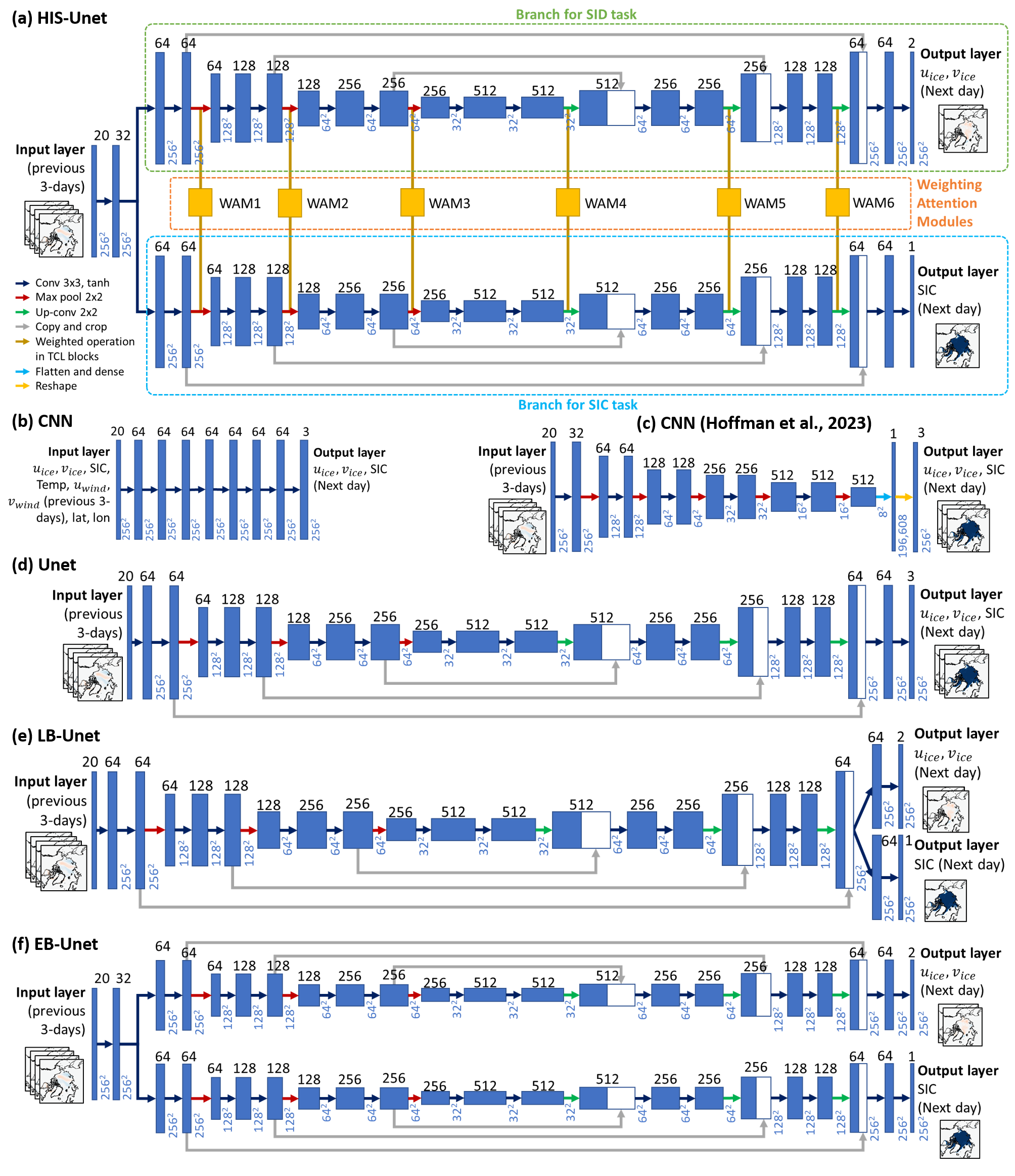
Figure 1: Architecture of six machine learning models: (a) Hierarchical information-sharing U-net (HIS-Unet), (b) Convolutional neural network (CNN) containing only convolutional layers, (c) CNN proposed by Hoffman et al. [24], (d) U-net, (e) late-branched U-net (LB-Unet), and (f) early-branched U-net (EB-Unet)

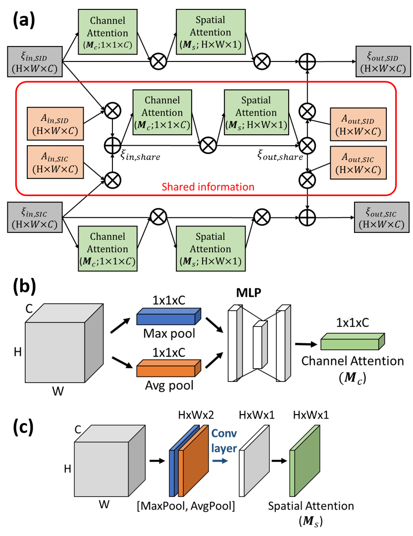
Figure 2: Schematic diagram of the (a) Weighting attention module (WAM), (b) Channel attention module, and (c) Spatial attention module.

IV-A Hierarchical information-sharing U-net

Fig 1a describes the architecture of the multi-task network we propose in this study: Hierarchical information-sharing U-net (HIS-Unet). In this architecture, two separate SID and SIC prediction tasks have their own branches of fully convolutional networks, only sharing the first convolutional layer of 32 filters. Each branch has a separate U-net construction [54] that produces SID and SIC, but they share and transfer their information through six weighting attention modules (WAMs). By adopting linear weighting parameters and channel/spatial attention modules in WAMs, we enable these WAMs to (1) determine how much information from SIC and SID is shared with each other and (2) focus on important channel and spatial information. We insert six WAMs right after the max pooling or up-convolution operations: three blocks in the encoder steps and three blocks in the decoder steps.

As shown in Fig 2a, each WAM receives information from SID and SIC branches and calculates the weighted sum of them. Letting a WAM receive the SID feature map ($\xi_{in,SID}$; image height $H$, image width $W$, channels $C$) and SIC feature map ($\xi_{in,SIC}$; $H\times W\times C$) from the previous max-pooling or up-convolution operations, the input shared information ($\xi_{in,share}$) is determined by following:

$$\xi_{in,share}=A_{in,SID}\xi_{in,SID}+A_{in,SIC}\xi_{in,SIC}$$ (3)

where $A_{in,SID}$ and $A_{in,SIC}$ denote the weights for the SID and SIC information, respectively. As indicators of the relative importance of SID and SIC, these weights are used to balance the effectiveness of information learned in the WAM.

After the input shared information $\xi_{in,share}$ is determined by the linear weighting combination of $\xi_{in,SID}$ and $\xi_{in,SIC}$, this shared information passes through channel attention module (Fig 2b) and spatial attention module (Fig 2c). The channel attention module and spatial attention module were proposed by [55] and have been widely used to improve the representation power of CNN networks. The channel attention highlights what channel is meaningful in a given input image, and the spatial attention highlights where an informative part is [55]. In the channel attention module, the spatial information of an input feature map is aggregated using max pooling and average pooling operations, and these two descriptors are forwarded to a multi-layer perceptron (MLP) with one hidden layer. Consequently, the channel attention map of $1\times 1\times C$ dimension is generated, and this channel attention map is multiplied with the input feature of $H\times W\times C$ dimension. After the channel attention is applied, the spatial attention is applied. In the spatial attention module, average pooling and max pooling are applied along the channel axis, and these two feature descriptors generate a spatial attention map ($H\times W\times C$ dimension) through a convolutional layer. This spatial attention map is also applied to the input image. Consequently, the input shared information $\xi_{in,share}$ is converted to the output shared information ($\xi_{out,share}$) via channel attention map and spatial attention map:

$$\xi_{out,share}=\boldsymbol{M}_{s}(\xi_{in,share})\otimes(\boldsymbol{M}_{c}(\xi_{in,share})\otimes\xi_{in,share})$$ (4)

where $\boldsymbol{M}_{s}$ and $\boldsymbol{M}_{c}$ denote spatial attention map and channel attention map, respectively, and $\otimes$ denotes element-wise multiplication. By arranging the channel attention and spatial attention sequentially, we can highlight what and where shared information is important. These channel and spatial attention modules are also applied to the input SID and SIC feature maps ($\xi_{in,SID}$ and $\xi_{in,SIC}$), as well as the shared information ($\xi_{in,share}$) in the WAM.

Then, the attention shared information is sent to the SID and SIC branches after multiplying output weights ($A_{out,SID}$ and $A_{out,SIC}$) and adding attention SID and SIC information, respectively:

$$\xi_{out,SID} =A_{out,SID}\xi_{out,share}$$ (5)

$$+\boldsymbol{M}_{s}(\xi_{in,SID})\otimes(\boldsymbol{M}_{c}(\xi_{in,SID})\otimes\xi_{in,SID})$$

$$\xi_{out,SIC} =A_{out,SIC}\xi_{out,share}$$ (6)

$$+\boldsymbol{M}_{s}(\xi_{in,SIC})\otimes(\boldsymbol{M}_{c}(\xi_{in,SIC})\otimes\xi_{in,SIC})$$

While $A_{in,SID}$ and $A_{in,SIC}$ determine the relative importance of entering information, $A_{out,SID}$ and $A_{out,SIC}$ determine how this shared information is significant for each branch. Since all weights have the same dimensions with the input matrix, these weights can imply the relative importance of SIC and SID for different pixel locations (see more details in section VI-B).

The objective loss function we use for learning is the sum of the mean square error (MSE) for u-component SIV ($u$), v-component SIV ($v$), and SIC ($A$):

$$Loss=\sum(\lvert u_{prd}-u_{obs}\rvert^{2}+\lvert v_{prd}-v_{obs}\rvert^{2}+\beta\lvert A_{prd}-A_{obs}\rvert^{2})$$ (7)

where the subscript $obs$ means observation and $prd$ means prediction, and $\beta$ is the weight for SIC MSE. $\beta$ is set to 0.5 for the multi-task network.

IV-B Baseline models

To compare with the HIS-Unet, we evaluate four neural network models and two simple statistical models. Four neural network models are (1) CNN only with convolutional layers, (2) CNN proposed by [24] for sea ice drift, (2) U-net, (3) Late-branched U-net (LB-Unet), and (4) Early-branched U-net (EB-Unet); two statistical models are (1) Persistence and (2) Linear regression (LR) models.

The first neural network model we evaluate is a CNN model consisting of 7 convolutional layers of 64 filters for each and an output layer with three channels of SID and SIC (Fig 1b). The second network we evaluate is the CNN architecture proposed by [24] (Fig 1c). This model consists of five sequential layers of convolutional and max pooling layers, followed by the flattening, dense, and reshaping layers. Since the original CNN model in [24] only predicts u- and v- component SID, we add an SIC output channel at the output layer.

The third network is the simple U-net proposed by Ronneberger et al. [54] (Fig 1d). The U-net is comprised of the encoder (contracting path) and decoder (expansive path). The encoder consists of repeated two $3\times 3$ convolutions and a $2\times 2$ max pooling operation with stride 2 for downsampling. The number of feature channels is doubled after each downsampling step. The decoder consists of several upsampling steps implemented by a $2\times 2$ up-convolution that halves the number of feature channels, a concatenation with the cropped feature map, and two $3\times 3$ convolutions [54]. Based on this U-net architecture, we also test a late-branched U-net (LB-Unet) (Fig 1e) and early-branched U-net (EB-Unet) (Fig 1f). The LB-Unet has the same architecture as the original U-net, but the last convolutional layer and output layer are branched for SID and SIC prediction separately. On the other hand, the EB-Unet only shares the first convolutional layer but the rest of the convolutional layers are independent for SID and SIC braches.

As a statistical model, the persistence model simply assumes that the sea ice condition remains the same as that of the previous day. The LR model, another statistical model, predicts $u$, $v$, and $A$ at pixel $(i,j)$ from the linear combination of the input variables as follows:

$$u(i,j)=\sum_{k=1}^{n}a_{u,k}(i,j)x_{k}(i,j)$$ (8)

$$v(i,j)=\sum_{k=1}^{n}a_{v,k}(i,j)x_{k}(i,j)$$ (9)

$$A(i,j)=\sum_{k=1}^{n}a_{A,k}(i,j)x_{k}(i,j)$$ (10)

where $n$ is the number of input variables and $x_{k}$ is the $k$th input variable. $a_{u,k}$, $a_{v,k}$, and $a_{A,k}$ are the linear coefficients corresponding to $x_{k}$ for the prediction of $u$, $v$, and $A$, respectively.

IV-C Evaluation metrics

The performances of the neural network models, statistical baseline models, and sea ice physics model are evaluated by the following three metrics: (1) Correlation coefficient (R), (2) Root mean square error (RMSE), and (3) Mean absolute error (MAE):

$$R=\frac{\sum(x-\overline{x})(y-\overline{y})}{\sqrt{\sum(x-\overline{x})^{2}\sum(y-\overline{y})^{2}}}$$ (11)

$$RMSE=\sqrt{\frac{(x-y)^{2}}{N}}$$ (12)

$$MAE=\sum\frac{\lvert x-y\rvert}{N}$$ (13)

where $x$ denotes the prediction values, $y$ denotes the observation values, and $N$ is the number of samples. In general, R can be useful to assess the overall spatiotemporal pattern of SIC and SID variations, and RMSE or MAE can be useful to assess the magnitude of prediction errors.

V Results

Table II: Accuracy of SIC and SIV prediction for each model

Model	Sea ice concentration (SIC)			Sea ice velocity (SIV)
	MAE (%)	RMSE (%)	R	MAE (km/d)	RMSE (km/d)	R
HIS-Unet	2.934	6.122	0.978	1.812	2.667	0.834
EB-Unet	3.139	6.238	0.974	1.926	2.773	0.818
LB-Unet	3.122	6.575	0.970	1.960	2.814	0.813
Unet	3.400	6.601	0.970	1.981	2.834	0.815
CNN	4.750	7.896	0.958	2.331	3.213	0.770
CNN [24]	10.071	16.963	0.839	2.223	3.217	0.742
LR	4.232	8.178	0.965	3.340	5.142	0.780
Persistence	3.135	7.435	0.924	2.871	4.181	0.629
HYCOM [53]	8.874	15.878	0.865	3.782	5.506	0.508

To predict the daily SID and SIC, we use the previous 3-days of SID (u- and v- components), SIC, air temperature, wind velocity (u- and v- components), and geographic location (i.e., x and y coordinates) as the inputs. Consequently, the input layer has 20 channels (three-day data of six sea ice or meteorological variables and two geographical variables) of $256\times 256$ grid size. All input values are normalized to -1 to 1 based on the nominal maximum and minimum values that each variable can have. Then, this model is trained to predict the SID and SIC for the next day. We collect the data from 2016 to 2022; 2016-2021 datasets are used to train/validate the model, and 2022 datasets are used to test the model. The 2016-2021 datasets are randomly divided into 80 % of train datasets and 20 % of validation datasets. The number of train, validation, and test datasets is 1742, 438, and 363, respectively. The kernel size of the convolutional layer is set to $3\times 3$ and the hyperbolic tangent (tanh) activation function is applied after each convolution. The HIS-Unet is trained to minimize the loss function in Eq.7 and optimized by Adam stochastic gradient descent algorithm [56] with 100 epochs and 0.001 learning rate. Such hyperparameter settings are the same for the other neural network models. We implement this model in Python using the PyTorch library. All scripts are executed on the GPU nodes of the Frontera supercomputing system from the Texas Advanced Computing Center (TACC), each node equipping four NVIDIA Quadro RTX 5000 GPUs of 16 GB memory.

Table II shows the test accuracy of sea ice concentration (SIC) and sea ice velocity (SIV) in 2022 for different models. The HIS-Unet model generally shows the best SIC and SIV prediction results, with the highest R (0.978 for SIC and 0.834 for SIV) and lowest RMSE (6.122 for SIC and 2.677 for SIV), followed by EB-Unet, LB-Unet, Unet, and CNN. The five fully convolutional neural network models (CNN, Unet, LB-Unet, EB-Unet, and HIS-Unet) show better performance than the persistence model for both SIC and SIV, suggesting that these models can significantly predict the daily variations of sea ice conditions. Additionally, these machine learning models outperform the LR model and HYCOM physical model. It is also worth mentioning that the CNN proposed by [24] has better fidelity than the persistence model in SIV but the worst performance in SIC prediction [24]. Since this CNN model was originally designed for only SIV prediction, this architecture does not produce reliable predictions for SIC.

The EB-Unet shows considerable improvement in both SIV and SIC prediction compared to LB-Unet and Unet. This implies that separating SIC and SIV information at the early-branch stage is more efficient in predicting both variables than using the late-branch architecture or adding channels at the output layer. However, considering that such an early-branch approach prevents information sharing at the intermediate learning stages, the information sharing between SIC and SID through WAMs in the middle of HIS-Unet architecture allows a better prediction for both SIC and SIV than the EB-Unet.

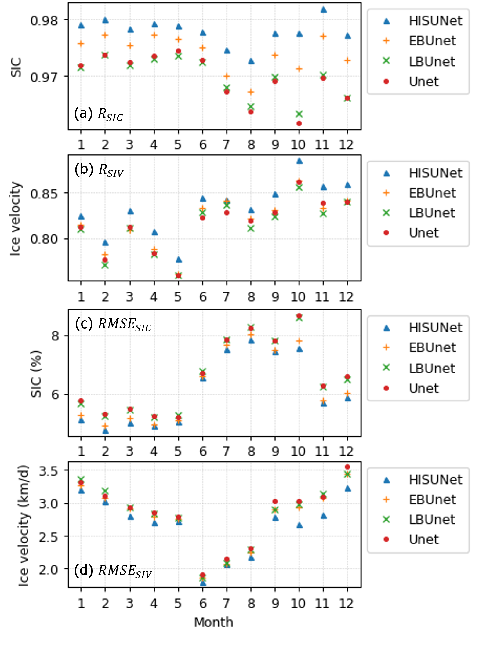
Figure 3: Comparison of monthly accuracy of the models in 2022: (a) R of SIC, (b) R of SIV, (c) RMSE of SIC, and (d) RMSE of SIV

Fig. 3 depicts the monthly accuracy for each model. It is notable that the HIS-Unet has remarkably better performance during all months in both SIC and SIV prediction. In particular, the correlation coefficient derived by HIS-Unet outperforms the other machine learning models in both SIC and SIV prediction, which supports that the HIS-Uent produces the spatiotemporal variations of SIC and SIV more successfully (Fig 3a and b). In terms of SIC prediction, the HIS-Unet shows a higher R by 0.002-0.006 and lower RMSE by 0.05-0.25 % compared to the EB-Unet. In particular, the largest improvement occurs in the summer months from July to October. While R varies significantly from July to October by other models ($<$ 0.97), the HIS-Unet keeps R $>$ 0.97 in these months, maintaining a similar level of R to winter months. October shows the most conspicuous improvement in SIC, reducing RMSE by 0.26 % and increasing R by 0.006. In general, the Arctic sea ice extent decreases rapidly in July and reaches the minimum in September. Then, sea ice starts to evolve from September, recording the fastest increasing rate in October. As a result, the thermodynamic and dynamic sea ice condition changes more abruptly in the summer months. Integrating SID information into SIC prediction via HIS-Unet might contribute to predicting SIC in this fast-melting and fast-growing season. Furthermore, as shown in Fig 4a, the improvement of R is observed near sea ice edges, rather than the central Arctic. This implies that SIV information can help predict spatiotemporal trends of SIC for where SIC changes much in melting and freezing seasons. On the other hand, regarding the RMSE value of the SIC prediction, the HIS-Unet also contributes to reducing SIC errors in the central Arctic (Fig 4b).

As for the SIV prediction, the R of HIS-Unet is higher than the EB-Unet by 0.01-0.02 and the RMSE is lower by 0.05-0.25 km/day on average. In the case of SIV, the largest improvement by HIS-Unet occurs in October-December: RMSE decreases more than 0.2 km/day, and R increases by 0.02. During these months, the Arctic sea ice extent starts to increase and sea ice becomes compacted. Such a compacted sea ice pack can either regulate or accelerate sea ice movement. Consequently, the integration of SIC information via HIS-Unet improves the SID prediction when sea ice compactness increases in October-December. Indeed, as shown in Fig 4c and d, the improvement of SIV prediction occurs at sea ice edges, not the central Arctic. The north of Greenland and the Canadian Archipelago are mainly covered by multi-year ice (MYI), which survives even in summer [57]. Thus, the SIC in the central Arctic does not change much over a year (see Fig 6c). Although the integration of SIC information via the HIS-Unet does not efficiently improve the SID predictability in the central Arctic, it improves the SID prediction broadly for the other regions where SIC changes seasonally.

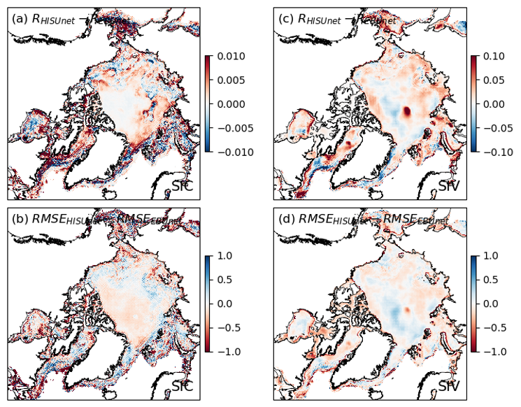
Figure 4: The difference of R and RMSE between HIS-Unet and EB-Unet: (a) R of SIC, (b) RMSE of SIC, (c) R of SIV, and (d) RMSE of SIV

VI Discussion

Considering that the interaction between SID and SIC can vary by sea ice conditions (e.g., sea ice edges v. central Arctic), it is worth comparing the model accuracy for different regions. Thus, in the following subsection VI-A, we discuss how the model accuracy changes for different regions of the Arctic Ocean. Furthermore, in subsection VI-B, we examine the characteristics of information sharing between SID and SIC layers, which occurs in WAMs.

VI-A Model accuracy for different Arctic subregions

We assess the accuracy of HIS-Unet for six different subregions in the Arctic Ocean (Fig. 5): Central Arctic (CA), Chukchi and Beaufort Seas (CBS), Laptev and East Siberian Seas (LESS), Kara and Barents Seas (KBS), East Greenland (EG), and Hudson and Baffin Bays (HBB). The division of these Arctic subregions has been conducted in many previous studies based on their unique atmospheric and sea ice characteristics [58]. Fig. 6 shows the RMSE and R of SIC and SIV prediction for these six subregions every month in 2022.

Regarding the SIC prediction, CA shows the most accurate prediction, with the highest R and lowest RMSE for all months. This should be because the CA region is almost covered by high-concentration sea ice all months (Fig 6c). Since SIC reaches almost 100 % for all seasons, the prediction of SIC in this region is relatively easier than in other regions. However, besides the CA region, all subregions show R values greater than 0.95 and RMSE less than 10 % for all seasons. The seasonal trend of SIC performance in CA, CBS, and LESS is slightly different from that in KBS, EG, and HBB. In CA, CBS, and LESS, the RMSE increases in the summer months from June to October. The lower SIC prediction performance in the summer months might be because SIC changes significantly in these regions during the summer months, accompanied by fast melting and fast growing (Fig 6c). When these three regions are entirely covered by sea ice from January to April, the RMSE of SIC is less than 2 % (Fig 6b). However, the SIC RMSEs in KBS, EG, and HBB are relatively higher than the other regions in winter months: the RMSEs in these regions from December to April reach up to 3-4 %. In the summer months, the RMSEs in KBS, EG, and HBB might be low just because of the wide ice-free area and low SIC.

Next, when it comes to the SIV prediction, it is interesting that the prediction performance is relatively stable in the CA region. While the other regions experience large fluctuations in R and RMSE values, the fluctuation of R and RMSE in CA is not as large as the other regions. The R-value remains 0.8-0.9 and RMSE 3.0-5.0 km/day for most of the months in CA. In CBS and LESS, the RMSE error of the SIV prediction increases in October-December, which might be attributed to a sudden increase in sea ice velocity in these regions (6f). Although the RMSE of SIV does not exceed 4.5 km/day in CBS and LESS before October, RMSE increases up to 6 km/day in October-December. The KBS and HBB subregions show abnormally high R and low RMSE values from July to October, but these values can be caused by very low sea ice covers (Fig 6c).

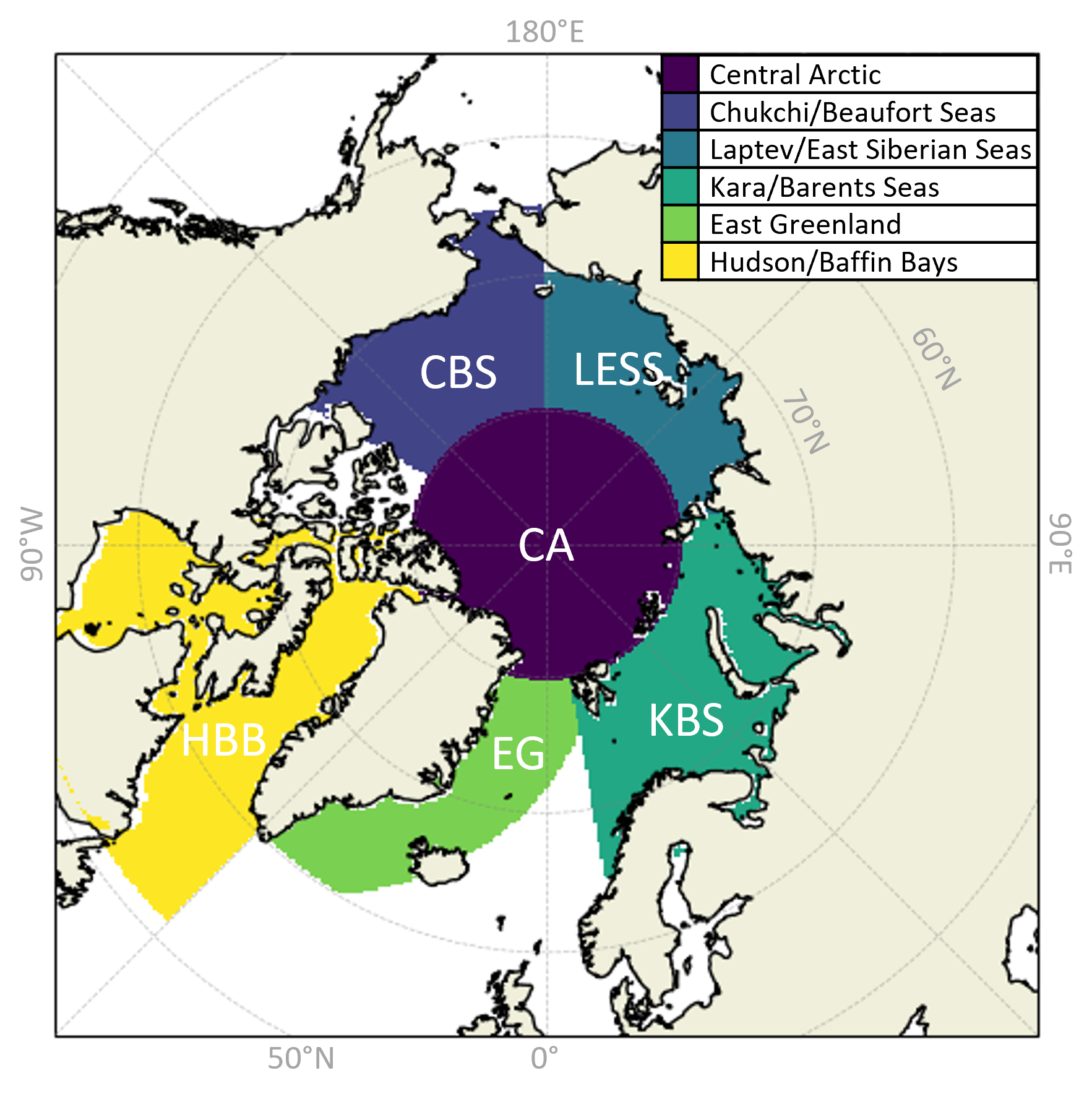
Figure 5: Six Arctic subregions defined in this study: Central Arctic (CA), Chukchi/Beaufort Seas (CBS), Laptev/East Siberian Seas (LESS), Kara/Barents Seas (KBS), East Greenland (EG), Hudson/Baffin Bays (HBB)

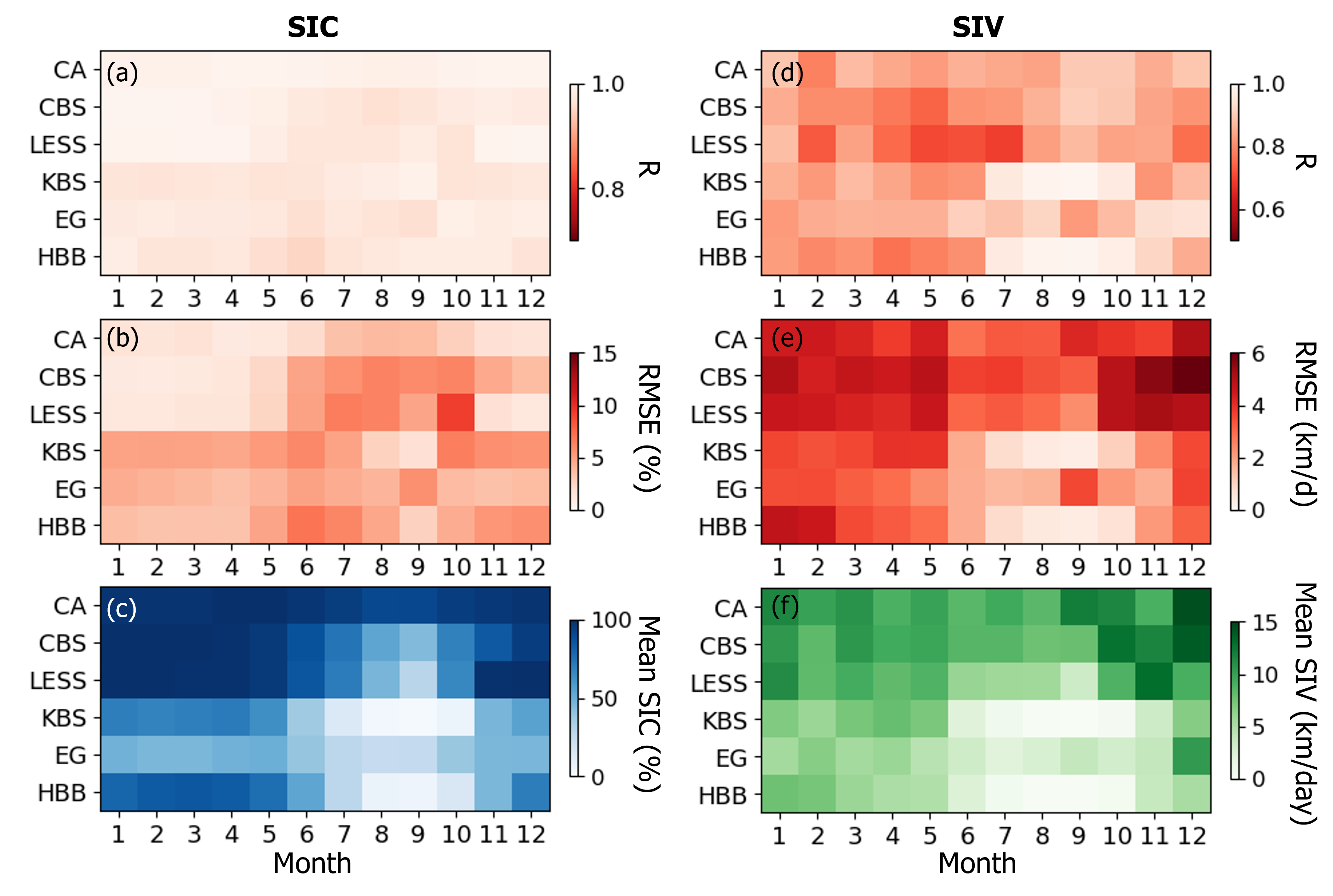
Figure 6: (a) R of SIC, (b) RMSE of SIC, and (c) mean SIC for six subregions; (d) R of SIV, (e) RMSE of SIV, and (f) mean SIV for six subregions

VI-B Characterization of information sharing pattern in weighting attention modules

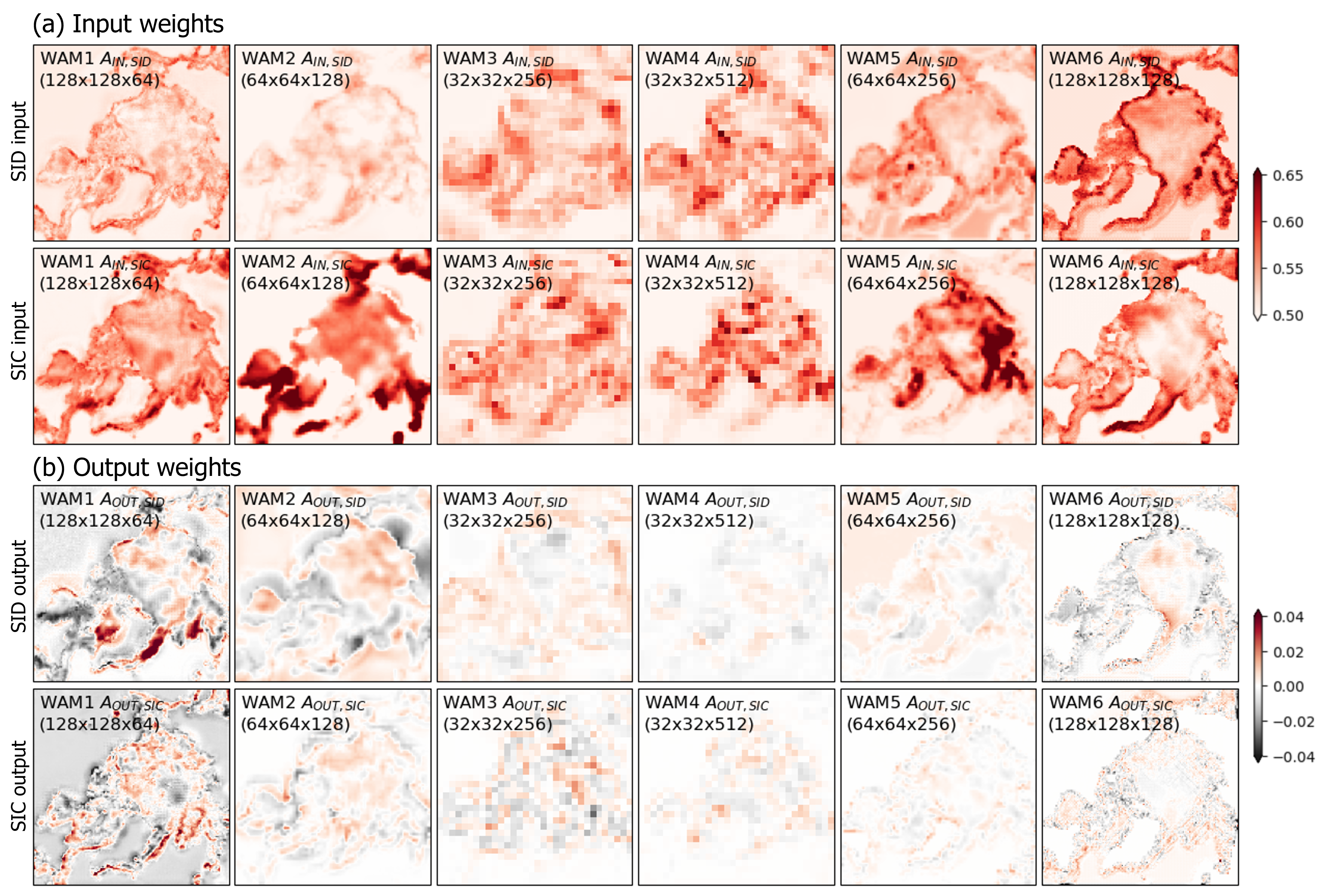
Figure 7: (a) WAM input weights ($A_{in,SID}$ and $A_{in,SIC}$) and (b) WAM output weights ($A_{out,SID}$ and $A_{out,SIC}$) in Fig 2a for each level of HIS-Unet in Fig 1a

In the HIS-Unet architecture we use in this study, WAM makes it possible for the SIC and SID prediction layers to share their information with each other. In the WAM, the information sharing is implemented by linear weight combination between SIC and SID layers followed by channel and spatial attention modules. Moreover, the output feature from this WAM is passed through the multiplication of the output weights before being transferred to each branch. These input and output weights determine how much SIC and SID information is to be mixed with each other and how significant this shared information is to be for each branch. Thus, we extract and examine the weight metrics of each WAM.

The input and output weights for WAM levels 1-6 are displayed in Fig 7a and b, respectively. Since each weight has the same dimension as the input layer ($H\times W\times C$), here we calculate the mean weights along all the channels ($H\times W$). As shown in Fig 7, the WAMs exhibit interesting patterns in weighting values and spatial distribution. In this section, we discuss the weighting values and spatial patterns exhibited in the WAM1, WAM2, WAM5, and WAM6 because their $H\times W$ dimension is closer to the original $256\times 256$ input and output dimension. There is a possibility that other intermediate WAMs represent fine-tuning the weights and biases in the model rather than weighted information sharing.

First, when the SID and SIC information are first blended through WAM1, SIC information is more weighted than SID with higher input weights. When this shared information is transferred to each branch, the shared information in the HBB, EG, and KBS regions is weighted in the SID branch, and the shared information in the EG and KBS regions is weighted in the SIC branch. In general, the magnitude of output weights is higher in the SID branch compared to the SIC branch.

At the next level of information sharing at WAM2, we find similar patterns between the SIC and SID branches: SIC information is more weighted in sharing information, and the SID branch receives more shared information in transferring the shared information. It is also interesting that the input SIC information is more weighted for sea ice edges near coastlines. This similar pattern is also observed in WAM5: more SIC contribution in shared information and strong transfer from shared information to the SID branch.

At the last information sharing state (WAM6), it is noted that the SID information is highlighted along the coastline in the information sharing. The SIC information is also more highlighted in the coastal regions than in the central Arctic. When the shared information transfers to each branch, the magnitude of output weights is also high along the coastlines, while the magnitude of weights in the central Arctic is close to zero.

Therefore, in summary, we find three noticeable characteristics in information sharing through WAMs of HIS-Unet: (1) information sharing between SIC and SID is relatively active in sea ice edges compared to the central Arctic, (2) when WAMs receive information from each branch and share them, SIC information is more weighted, (3) when WAMs pass the sharing information to each branch, the shared information becomes more critical for the SID branch.

VII Conclusion

In this study, we propose a multi-task fully convolutional network to predict Arctic sea ice concentration (SIC) and sea ice drift (SID). We accomplish the information sharing between SIC and SID layers by adding six weighting attention modules (WAMs) between separate SIC and SID U-net branches. The intermediate feature maps from each branch enter a WAM with input weights, and the outputs from the WAM are transferred to each branch with output weights. Considering that SIC and SID affect each other in thermodynamic and dynamic ways, the information sharing and attention through WAMs can indirectly allow the network to learn their complicated interactions. Indeed, our hierarchical information-sharing U-net (HIS-Unet) shows better performance than other network architectures, including convolutional network, U-net, late-branched U-net (LB-Unet), and early-branched U-net (EB-Unet). In particular, our HIS-Unet outperforms these models in the melting season and early freezing season. The HIS-Unet shows a stable performance in the central Arctic, where the SIC is relatively stable throughout the year. For the other regions, although the model performance varies by the sea ice conditions, the fidelity of HIS-Unet is close to or better than the previous SIC and SID prediction studies. As the first attempt to predict SIC and SID simultaneously, the information sharing through WAMs shows the potential to improve the predictability of both SIC and SID. According to the input and output weight values and the prediction result of the HIS-Unet, the information-sharing scheme plays an important role in predicting SIC and SID when sea ice conditions change fast at the sea ice edges.

Younghyun Koo received the B.S. degree in Energy resources engineering from Seoul National University, Republic of Korea, in 2017, the M.S degree in Energy systems engineering from Seoul National University, Republic of Korea, in 2019, and the Ph.D degree in Environmental Science and Engineering from the University of Texas at San Antonio, TX, USA, in 2023. He is currently a postdoctoral research associate at the Computer Vision and Remote Sensing Laboratory (Bina lab) at Lehigh University. His research interest is the application of machine learning and remote sensing techniques for environmental monitoring, particularly in polar regions. His research is funded by the U.S. National Science Foundation (NSF).

Maryam Rahnemoonfar received her Ph.D. degree in Computer Science from the University of Salford, Manchester, U.K. She is currently an Associate Professor and Director of the Computer Vision and Remote Sensing Laboratory (Bina lab) at Lehigh University. Her research interests include Deep Learning, Computer Vision, Data Science, AI for Social Good, Remote Sensing, and Document Image Analysis. Her research specifically focuses on developing novel machine learning and computer vision algorithms for heterogeneous sensors such as Radar, Sonar, Multi-spectral, and Optical. Her research has been funded by several awards including the NSF HDR Institute award-iHARP, NSF BIGDATA award, Amazon Academic Research Award, Amazon Machine Learning award, Microsoft, and IBM.

References

- [1] D. J. Cavalieri and C. L. Parkinson, “Arctic sea ice variability and trends, 1979-2010,” The Cryosphere, vol. 6, no. 4, pp. 881–889, 2012.
- [2] J. C. Stroeve, V. Kattsov, A. Barrett, M. Serreze, T. Pavlova, M. Holland, and W. N. Meier, “Trends in arctic sea ice extent from cmip5, cmip3 and observations,” Geophysical Research Letters, vol. 39, no. 16, 2012.
- [3] D. Notz and J. Stroeve, “Observed arctic sea-ice loss directly follows anthropogenic co¡sub¿2¡/sub¿ emission,” Science, vol. 354, no. 6313, pp. 747–750, 2016.
- [4] I. H. Onarheim, T. Eldevik, L. H. Smedsrud, and J. C. Stroeve, “Seasonal and regional manifestation of arctic sea ice loss,” Journal of Climate, vol. 31, no. 12, pp. 4917 – 4932, 2018.
- [5] R. Lindsay and A. Schweiger, “Arctic sea ice thickness loss determined using subsurface, aircraft, and satellite observations,” The Cryosphere, vol. 9, no. 1, pp. 269–283, 2015.
- [6] R. Kwok, “Arctic sea ice thickness, volume, and multiyear ice coverage: losses and coupled variability (1958–2018),” Environmental Research Letters, vol. 13, p. 105005, oct 2018.
- [7] X. Yu, A. Rinke, W. Dorn, G. Spreen, C. Lüpkes, H. Sumata, and V. M. Gryanik, “Evaluation of arctic sea ice drift and its dependency on near-surface wind and sea ice conditions in the coupled regional climate model hirham–naosim,” The Cryosphere, vol. 14, no. 5, pp. 1727–1746, 2020.
- [8] R. Kwok, G. Spreen, and S. Pang, “Arctic sea ice circulation and drift speed: Decadal trends and ocean currents,” Journal of Geophysical Research: Oceans, vol. 118, no. 5, pp. 2408–2425, 2013.
- [9] J. Anheuser, Y. Liu, and J. R. Key, “A climatology of thermodynamic vs. dynamic arctic wintertime sea ice thickness effects during the cryosat-2 era,” The Cryosphere, vol. 17, no. 7, pp. 2871–2889, 2023.
- [10] T. J. W. Wagner, I. Eisenman, and H. C. Mason, “How sea ice drift influences sea ice area and volume,” Geophysical Research Letters, vol. 48, no. 19, p. e2021GL093069, 2021. e2021GL093069 2021GL093069.
- [11] E. Blockley, M. Vancoppenolle, E. Hunke, C. Bitz, D. Feltham, J.-F. Lemieux, M. Losch, E. Maisonnave, D. Notz, P. Rampal, S. Tietsche, B. Tremblay, A. Turner, F. Massonnet, E. Ólason, A. Roberts, Y. Aksenov, T. Fichefet, G. Garric, D. Iovino, G. Madec, C. Rousset, D. S. y Melia, and D. Schroeder, “The future of sea ice modeling: Where do we go from here?,” Bulletin of the American Meteorological Society, vol. 101, no. 8, pp. E1304 – E1311, 2020.
- [12] E. C. Hunke, W. H. Lipscomb, and A. K. Turner, “Sea-ice models for climate study: retrospective and new directions,” Journal of Glaciology, vol. 56, no. 200, p. 1162–1172, 2010.
- [13] E. Blanchard-Wrigglesworth, R. I. Cullather, W. Wang, J. Zhang, and C. M. Bitz, “Model forecast skill and sensitivity to initial conditions in the seasonal sea ice outlook,” Geophysical Research Letters, vol. 42, no. 19, pp. 8042–8048, 2015.
- [14] T. R. Andersson, J. S. Hosking, M. Pérez-Ortiz, B. Paige, A. Elliott, C. Russell, S. Law, D. C. Jones, J. Wilkinson, T. Phillips, J. Byrne, S. Tietsche, B. B. Sarojini, E. Blanchard-Wrigglesworth, Y. Aksenov, R. Downie, and E. Shuckburgh, “Seasonal arctic sea ice forecasting with probabilistic deep learning,” Nature Communications, vol. 12, no. 5124, 2021.
- [15] Y. J. Kim, H.-C. Kim, D. Han, S. Lee, and J. Im, “Prediction of monthly arctic sea ice concentrations using satellite and reanalysis data based on convolutional neural networks,” The Cryosphere, vol. 14, no. 3, pp. 1083–1104, 2020.
- [16] Y. Ren and X. Li, “Predicting daily arctic sea ice concentration in the melt season based on a deep fully convolution network model,” in 2021 IEEE International Geoscience and Remote Sensing Symposium IGARSS, pp. 5540–5543, 2021.
- [17] Y. Ren, X. Li, and W. Zhang, “A data-driven deep learning model for weekly sea ice concentration prediction of the pan-arctic during the melting season,” IEEE Transactions on Geoscience and Remote Sensing, vol. 60, pp. 1–19, 2022.
- [18] J. Wei, R. Hang, and J.-J. Luo, “Prediction of pan-arctic sea ice using attention-based lstm neural networks,” Frontiers in Marine Science, vol. 9, 2022.
- [19] Q. Liu, R. Zhang, Y. Wang, H. Yan, and M. Hong, “Daily prediction of the arctic sea ice concentration using reanalysis data based on a convolutional lstm network,” Journal of Marine Science and Engineering, vol. 9, no. 3, 2021.
- [20] Q. Zheng, W. Li, Q. Shao, G. Han, and X. Wang, “A mid- and long-term arctic sea ice concentration prediction model based on deep learning technology,” Remote Sensing, vol. 14, no. 12, 2022.
- [21] Y. Liu, L. Bogaardt, J. Attema, and W. Hazeleger, “Extended-range arctic sea ice forecast with convolutional long short-term memory networks,” Monthly Weather Review, vol. 149, no. 6, pp. 1673 – 1693, 2021.
- [22] J. Chi and H.-c. Kim, “Prediction of arctic sea ice concentration using a fully data driven deep neural network,” Remote Sensing, vol. 9, no. 12, 2017.
- [23] B. Mu, X. Luo, S. Yuan, and X. Liang, “Icetft v1.0.0: interpretable long-term prediction of arctic sea ice extent with deep learning,” Geoscientific Model Development, vol. 16, no. 16, pp. 4677–4697, 2023.
- [24] L. Hoffman, M. R. Mazloff, S. T. Gille, D. Giglio, C. M. Bitz, P. Heimbach, and K. Matsuyoshi, “Machine learning for daily forecasts of arctic sea-ice motion: an attribution assessment of model predictive skill,” Artificial Intelligence for the Earth Systems, pp. 1 – 45, 2023.
- [25] J. Zhai and C. M. Bitz, “A machine learning model of arctic sea ice motions,” 2021.
- [26] P. R. Holland and R. Kwok, “Wind-driven trends in antarctic sea-ice drift,” Nature Geoscience, vol. 5, pp. 872–875, 2012.
- [27] P. R. Holland and N. Kimura, “Observed concentration budgets of arctic and antarctic sea ice,” Journal of Climate, vol. 29, no. 14, pp. 5241 – 5249, 2016.
- [28] W. D. Hibler, “A dynamic thermodynamic sea ice model,” Journal of Physical Oceanography, vol. 9, no. 4, pp. 815 – 846, 1979.
- [29] A. S. Thorndike and R. Colony, “Sea ice motion in response to geostrophic winds,” Journal of Geophysical Research: Oceans, vol. 87, no. C8, pp. 5845–5852, 1982.
- [30] M. Ken, K. Noriaki, and Y. Hajime, “Temporal and spatial change in the relationship between sea-ice motion and wind in the arctic,” Polar Research, vol. 39, Nov. 2020.
- [31] Q. Liu, R. Zhang, Y. Wang, H. Yan, and M. Hong, “Short-term daily prediction of sea ice concentration based on deep learning of gradient loss function,” Frontiers in Marine Science, vol. 8, 2021.
- [32] Z. I. Petrou and Y. Tian, “Prediction of sea ice motion with convolutional long short-term memory networks,” IEEE Transactions on Geoscience and Remote Sensing, vol. 57, no. 9, pp. 6865–6876, 2019.
- [33] M. Crawshaw, “Multi-task learning with deep neural networks: A survey,” CoRR, vol. abs/2009.09796, 2020.
- [34] H. Alhichri, “Multitask classification of remote sensing scenes using deep neural networks,” in IGARSS 2018 - 2018 IEEE International Geoscience and Remote Sensing Symposium, pp. 1195–1198, 2018.
- [35] M. Papadomanolaki, M. Vakalopoulou, and K. Karantzalos, “A deep multitask learning framework coupling semantic segmentation and fully convolutional lstm networks for urban change detection,” IEEE Transactions on Geoscience and Remote Sensing, vol. 59, no. 9, pp. 7651–7668, 2021.
- [36] M. Ilteralp, S. Ariman, and E. Aptoula, “A deep multitask semisupervised learning approach for chlorophyll-a retrieval from remote sensing images,” Remote Sensing, vol. 14, no. 1, 2022.
- [37] M. Li, J. Long, A. Stein, and X. Wang, “Using a semantic edge-aware multi-task neural network to delineate agricultural parcels from remote sensing images,” ISPRS Journal of Photogrammetry and Remote Sensing, vol. 200, pp. 24–40, 2023.
- [38] K. He, C. Lian, B. Zhang, X. Zhang, X. Cao, D. Nie, Y. Gao, J. Zhang, and D. Shen, “Hf-unet: Learning hierarchically inter-task relevance in multi-task u-net for accurate prostate segmentation in ct images,” IEEE Transactions on Medical Imaging, vol. 40, no. 8, pp. 2118–2128, 2021.
- [39] I. Misra, A. Shrivastava, A. Gupta, and M. Hebert, “Cross-stitch networks for multi-task learning,” in 2016 IEEE Conference on Computer Vision and Pattern Recognition (CVPR), (Los Alamitos, CA, USA), pp. 3994–4003, IEEE Computer Society, jun 2016.
- [40] S. Ruder, J. Bingel, I. Augenstein, and A. Søgaard, “Latent multi-task architecture learning,” in Proceedings of the Thirty-Third AAAI Conference on Artificial Intelligence and Thirty-First Innovative Applications of Artificial Intelligence Conference and Ninth AAAI Symposium on Educational Advances in Artificial Intelligence, AAAI’19/IAAI’19/EAAI’19, AAAI Press, 2019.
- [41] Y. Gao, J. Ma, M. Zhao, W. Liu, and A. L. Yuille, “Nddr-cnn: Layerwise feature fusing in multi-task cnns by neural discriminative dimensionality reduction,” in 2019 IEEE/CVF Conference on Computer Vision and Pattern Recognition (CVPR), (Los Alamitos, CA, USA), pp. 3200–3209, IEEE Computer Society, jun 2019.
- [42] M. A. Tschudi, W. N. Meier, and J. S. Stewart, “An enhancement to sea ice motion and age products at the national snow and ice data center (nsidc),” The Cryosphere, vol. 14, no. 5, pp. 1519–1536, 2020.
- [43] W. N. Meier, F. Fetterer, A. K. Windnagel, and J. S. Stewart, “Noaa/nsidc climate data record of passive microwave sea ice concentration, version 4,” 2021.
- [44] H. Hersbach, B. Bell, P. Berrisford, S. Hirahara, A. Horányi, J. Muñoz-Sabater, J. Nicolas, C. Peubey, R. Radu, D. Schepers, A. Simmons, C. Soci, S. Abdalla, X. Abellan, G. Balsamo, P. Bechtold, G. Biavati, J. Bidlot, M. Bonavita, G. De Chiara, P. Dahlgren, D. Dee, M. Diamantakis, R. Dragani, J. Flemming, R. Forbes, M. Fuentes, A. Geer, L. Haimberger, S. Healy, R. J. Hogan, E. Hólm, M. Janisková, S. Keeley, P. Laloyaux, P. Lopez, C. Lupu, G. Radnoti, P. de Rosnay, I. Rozum, F. Vamborg, S. Villaume, and J.-N. Thépaut, “The era5 global reanalysis,” Quarterly Journal of the Royal Meteorological Society, vol. 146, no. 730, pp. 1999–2049, 2020.
- [45] M. Tschudi, J. S. Meier, W. N. Stewart, C. Fowler, and J. Maslanik, “Polar pathfinder daily 25 km ease-grid sea ice motion vectors, version 4,” 2019.
- [46] D. J. Cavalieri, P. Gloersen, and W. J. Campbell, “Determination of sea ice parameters with the nimbus 7 smmr,” Journal of Geophysical Research: Atmospheres, vol. 89, no. D4, pp. 5355–5369, 1984.
- [47] J. C. Comiso, “Characteristics of arctic winter sea ice from satellite multispectral microwave observations,” Journal of Geophysical Research: Oceans, vol. 91, no. C1, pp. 975–994, 1986.
- [48] W. Meier, “Comparison of passive microwave ice concentration algorithm retrievals with avhrr imagery in arctic peripheral seas,” IEEE Transactions on Geoscience and Remote Sensing, vol. 43, no. 6, pp. 1324–1337, 2005.
- [49] J. C. Comiso, D. J. Cavalieri, C. L. Parkinson, and P. Gloersen, “Passive microwave algorithms for sea ice concentration: A comparison of two techniques,” Remote Sensing of Environment, vol. 60, no. 3, pp. 357–384, 1997.
- [50] N. Ivanova, L. T. Pedersen, R. T. Tonboe, S. Kern, G. Heygster, T. Lavergne, A. Sørensen, R. Saldo, G. Dybkjær, L. Brucker, and M. Shokr, “Inter-comparison and evaluation of sea ice algorithms: towards further identification of challenges and optimal approach using passive microwave observations,” The Cryosphere, vol. 9, no. 5, pp. 1797–1817, 2015.
- [51] S. Kern, T. Lavergne, D. Notz, L. T. Pedersen, and R. Tonboe, “Satellite passive microwave sea-ice concentration data set inter-comparison for arctic summer conditions,” The Cryosphere, vol. 14, no. 7, pp. 2469–2493, 2020.
- [52] P. Sakov, F. Counillon, L. Bertino, K. A. Lisæter, P. R. Oke, and A. Korablev, “Topaz4: an ocean-sea ice data assimilation system for the north atlantic and arctic,” Ocean Science, vol. 8, no. 4, pp. 633–656, 2012.
- [53] E. P. Chassignet, H. E. Hurlburt, O. M. Smedstad, G. R. Halliwell, P. J. Hogan, A. J. Wallcraft, R. Baraille, and R. Bleck, “The hycom (hybrid coordinate ocean model) data assimilative system,” Journal of Marine Systems, vol. 65, no. 1, pp. 60–83, 2007. Marine Environmental Monitoring and Prediction.
- [54] O. Ronneberger, P. Fischer, and T. Brox, “U-net: Convolutional networks for biomedical image segmentation,” in Medical Image Computing and Computer-Assisted Intervention – MICCAI 2015 (N. Navab, J. Hornegger, W. M. Wells, and A. F. Frangi, eds.), (Cham), pp. 234–241, Springer International Publishing, 2015.
- [55] S. Woo, J. Park, J.-Y. Lee, and I. S. Kweon, “Cbam: Convolutional block attention module,” in Computer Vision – ECCV 2018 (V. Ferrari, M. Hebert, C. Sminchisescu, and Y. Weiss, eds.), (Cham), pp. 3–19, Springer International Publishing, 2018.
- [56] D. P. Kingma and J. Ba, “Adam: A method for stochastic optimization,” in 3rd International Conference on Learning Representations, ICLR 2015, San Diego, CA, USA, May 7-9, 2015, Conference Track Proceedings (Y. Bengio and Y. LeCun, eds.), 2015.
- [57] W. N. Meier and J. Stroeve, “An updated assessment of the changing arctic sea ice cover,” Oceanography, vol. 35, no. 3/4, pp. pp. 10–19, 2022.
- [58] C. L. Parkinson, D. J. Cavalieri, P. Gloersen, H. J. Zwally, and J. C. Comiso, “Arctic sea ice extents, areas, and trends, 1978–1996,” Journal of Geophysical Research: Oceans, vol. 104, no. C9, pp. 20837–20856, 1999.