Abstract

The review presents the methods of generation of nonlinear coherent excitations in strongly nonequilibrium Bose-condensed systems of trapped atoms and their properties. Non-ground-state Bose-Einstein condensates are represented by nonlinear coherent modes. The principal difference of nonlinear coherent modes from linear collective excitations is emphasized. Methods of generating nonlinear modes and the properties of the latter are described. Matter-wave interferometry with coherent modes is discussed, including such effects as interference patterns, internal Josephson current, Rabi oscillations, Ramsey fringes, harmonic generation, and parametric conversion. Dynamic transition between mode-locked and mode-unlocked regimes is shown to be analogous to a phase transition. Atomic squeezing and entanglement in a lattice of condensed atomic clouds with coherent modes are considered. Nonequilibrium states of trapped Bose-condensed systems, starting from weakly nonequilibrium state, vortex state, vortex turbulence, droplet or grain turbulence, and wave turbulence, are classified by means of effective Fresnel and Mach numbers. The inverse Kibble-Zurek scenario is described. A method for the formation of directed beams from atom lasers is reported.

Keywords: non-ground-state Bose-Einstein condensates, coherent modes, resonant generation, resonant entanglement, atomic squeezing, quantum turbulence, atom laser

Contents

1. Introduction

2. Condensate wave function

3. Coherent modes

4. Resonant generation

5. Counterflow instability

6. Energy levels

7. Mode dynamics

8. Mode locking

9. Shape-conservation criterion

10. Multiple mode generation

11. Matter-wave interferometry

11.1. Interference patterns

11.2. Internal Josephson current

11.3. Rabi oscillations

11.4. Higher-order resonances

12. Ramsey fringes

13. Interaction modulation

14. Strong interactions and noise

15. Critical phenomena

16. Atomic squeezing

17. Cloud entanglement

17.1. Entangled states

17.2. Entanglement production

17.3. Resonant entanglement production

18. Nonresonant mode generation

19. Nonequilibrium states

19.1. Weak nonequilibrium

19.2. Vortex embryos

19.3. Vortex rings

19.4. Vortex lines

19.5. Vortex turbulence

19.6. Droplet state

19.7. Wave turbulence

20. Classification of states

21. Atom laser

22. Conclusion

1 Introduction

Bose-Einstein condensation of trapped dilute atoms has been of high interest in recent years [1, 2, 3] since 1995, triggering voluminous publications, as can be inferred from review articles [4, 5, 6, 7, 8, 9, 10, 11, 12, 13, 14, 15, 16]. Equilibrium states of Bose-condensed systems have been studied both for atoms in traps and in optical lattices [17, 18, 19, 20, 21]. Elementary excitations have been investigated, corresponding to small deviations from the ground state, that is, to small density oscillations. These excitations are usually described by considering linear deviations of density from the ground state.

In 1997, the authors [22] suggested that it is feasible to generate in atomic traps strongly nonlinear excitations corresponding to non-ground-state Bose-Einstein condensates. Since the state of condensed atoms is equivalent to a coherent state [23], these nonlinear excitations are called nonlinear coherent modes. These modes enjoy several important properties allowing for the realization of interesting effects. A trapped Bose condensate with nonlinear coherent modes reminds an atom with several energy levels that can be connected by resonant electromagnetic field. Therefore a condensate with coherent modes allows for the occurrence of effects similar to those happening for atoms, such as Rabi oscillations, appearance of interference patterns, Josephson current, and Ramsey fringes. There also exist the effects of harmonic generation and parametric conversion.

At the same time, a Bose-condensed atomic system is nonlinear due to interactions between atoms, and it possesses highly nontrivial dynamics of coherent modes. It demonstrates different regimes of motion. In a Bose-condensed system, there is a mode-locked regime, when the modes are locked, so that their fractional populations vary only in a part of the whole admissible region. The other is mode-unlocked regime, when the mode populations vary in the whole admissible interval. The dynamic transition between these regimes is analogous to a phase transition in a statistical system. In a three-mode system, there can occurs the regime of chaotic motion, which is not possible in a two-mode system.

For Bose-condensed system of trapped atoms, it is possible to realize collective squeezing effects. Simultaneous generation of coherent modes in several connected traps, such as deep optical latices, allows for the creation of entangled mesoscopic clouds and for the study of the effect of resonant entanglement production.

Coherent atomic clouds released from a trap form what is called atom laser. The difference of an atom laser from the photonic laser is that atoms fall down due to gravity, but cannot be forwarded in the desired direction. However, realizing special initial conditions one can trigger the beam emanation in any chosen direction.

Nonequilibrium states can also be generated by strong nonresonant pumping creating such coherent modes as quantum rings and vortices. Strong pumping leads to the generation of vortex turbulence. Then there happens the formation of droplets of Bose condensate floating among uncondensed atoms, and droplet (or grain) turbulence develops. Even more strong pumping results in the destruction of condensate and wave turbulence. The overall process of consecutive generation of nonequilibrium states from an equilibrium condensate through ring and vortex states, to vortex and droplet turbulence, and ending with uncondensed state, has been named inverse Kibble-Zurek scenario. A classification of nonequilibrium states is advanced, by means of relative injected energy, effective temperature, Fresnel and Mach numbers.

Below, we use the system of units, where the Planck and Boltzmann constants are set to one.

2 Condensate wave function

Atomic systems Bose-condensed in traps are usually rather rarified, such that the effective interaction radius $r_{int}$ is much smaller than the mean interparticle distance $a$, which can be written as

$$\frac{r_{int}}{a}~{}\ll~{}1\;,\qquad\rho^{1/3}r_{int}~{}\ll~{}1\;,$$ (1)

where $\rho\sim a^{-3}$ is the average density of particles. At the same time the effective strength of particle interactions

$$\gamma~{}\equiv~{}\rho^{1/3}a_{s}$$ (2)

can be large, with $a_{s}$ being scattering length. In that sense, the rarified system of trapped atoms is a gas cloud.

The energy Hamiltonian has the standard form

$$\hat{H}~{}=~{}\int\psi^{\dagger}({\bf r})\;\left(-\;\frac{\nabla^{2}}{2m}+U\right)\;\psi({\bf r})\;d{\bf r}~{}+~{}\frac{1}{2}\int\psi^{\dagger}({\bf r})\;\psi^{\dagger}({\bf r}^{\prime})\;\Phi({\bf r}-{\bf r}^{\prime})\;\psi({\bf r}^{\prime})\;\psi({\bf r})\;d{\bf r}d{\bf r}^{\prime}\;,$$ (3)

where $U=U({\bf r},t)$ is an external trapping potential. Short-range interactions of rarified atoms can be represented by the effective interaction potential

$$\Phi({\bf r})~{}=~{}\Phi_{0}\delta({\bf r})\qquad\left(\Phi_{0}~{}\equiv~{}4\pi\;\frac{a_{s}}{m}\right)\;.$$ (4)

The Heisenberg equation of motion for the field operator reads as

$$i\;\frac{\partial}{\partial t}\;\psi({\bf r},t)~{}=~{}H[\;\psi\;]\;\psi({\bf r},t)\;,$$ (5)

with the effective nonlinear Hamiltonian

$$H[\;\psi\;]~{}\equiv~{}-\;\frac{\nabla^{2}}{2m}+U({\bf r},t)+\int\psi^{\dagger}({\bf r}^{\prime})\;\Phi({\bf r}-{\bf r}^{\prime})\;\psi({\bf r}^{\prime})\;d{\bf r}^{\prime}\;.$$ (6)

Bose-Einstein condensation means the appearance of a coherent state. At asymptotically low temperature, such that

$$T~{}\ll~{}\rho\Phi_{0}\;,$$ (7)

and very weak interactions, when

$$\gamma~{}\ll~{}1\;,$$ (8)

almost all atoms are Bose condensed, hence practically all the system is in a coherent state.

Coherent states are the eigenstates of the annihilation field operator $\psi({\bf r},t)$,

$$\psi({\bf r},t)\;|\;\eta\;\rangle~{}=~{}\eta({\bf r},t)\;|\;\eta\;\rangle\;,$$ (9)

with $\eta({\bf r},t)$ being called the coherent field or condensate wave function. The coherent field is the vacuum state of a Bose-condensed system [23]. Averaging Eq. (5) over the vacuum coherent state yields the equation for the condensate function (coherent field)

$$i\;\frac{\partial}{\partial t}\;\eta({\bf r},t)~{}=~{}H[\;\eta\;]\;\eta({\bf r},t)\;,$$ (10)

where the nonlinear Hamiltonian is

$$H[\;\eta\;]~{}=~{}-\;\frac{\nabla^{2}}{2m}+U({\bf r},t)+\int\Phi({\bf r}-{\bf r}^{\prime})\;|\;\eta({\bf r}^{\prime},t)\;|^{2}d{\bf r}^{\prime}\;.$$ (11)

This equation, for an arbitrary interaction potential, was advanced by Bogolubov in his book [24] that has been republished numerous times (see, e.g. [25, 26, 27]) and studied in Refs. [28, 29, 30, 31, 32, 33, 34]. By its mathematical structure, this is a nonlinear Schrödinger equation [35]. For trapped atoms with the interaction potential (4), it reads as

$$i\;\frac{\partial}{\partial t}\;\eta({\bf r},t)~{}=~{}\left[\;-\;\frac{\nabla^{2}}{2m}+U({\bf r},t)+\Phi_{0}\;|\;\eta({\bf r},t)\;|^{2}\;\right]\;\eta({\bf r},t)\;.$$ (12)

The condensate function is normalized to the total number of atoms,

$$\int|\;\eta({\bf r},t)\;|^{2}\;d{\bf r}~{}=~{}N\;.$$

Recall that this equation assumes that all atoms are Bose-condensed and temperature is zero, therefore it can provide a reasonable approximation only for very low temperatures and asymptotically weak interactions, when inequalities (7) and (8) are valid.

Since the number of atoms $N$ is conserved, it is possible to make the replacement

$$\eta({\bf r},t)~{}=~{}\sqrt{N}\;\varphi({\bf r},t)\;,$$ (13)

so that the normalization condition becomes

$$\int|\;\varphi({\bf r},t)\;|^{2}\;d{\bf r}~{}=~{}1\;.$$

The external potential can be separated into a constant part of a trapping potential and its temporal modulation,

$$U({\bf r},t)~{}=~{}U({\bf r})+V({\bf r},t)\;.$$ (14)

Thus we come to the equation

$$i\;\frac{\partial}{\partial t}\;\varphi({\bf r},t)~{}=~{}\left[\;\hat{H}[\;\varphi\;]+V({\bf r},t)\;\right]\;\varphi({\bf r},t)\;,$$ (15)

with a nonlinear Hamiltonian

$$\hat{H}[\;\varphi\;]~{}=~{}-\;\frac{\nabla^{2}}{2m}+U({\bf r})+N\Phi_{0}\;|\;\varphi({\bf r},t)\;|^{2}\;.$$ (16)

The Cauchy problem (15), generally speaking, does not have a unique solution, since it does not satisfy the conditions of the Cauchy-Kovalevskaya theorem [36]. To find uniquely defined solutions, one has to concretize the sought class of functions [37, 38]. We shall be looking for nonlinear solutions that can be treated as analytical continuation for the solutions of the linear Schrödinger equation.

3 Coherent modes

Let us consider the stationary solutions to Eq. (15). Substituting in (12) the expression

$$\eta({\bf r},t)~{}=~{}\eta({\bf r})e^{-iEt}$$ (17)

gives the stationary eigenproblem

$$\hat{H}[\;\varphi_{n}\;]\;\varphi_{n}({\bf r})~{}=~{}E_{n}\;\varphi_{n}({\bf r})$$ (18)

defining a spectrum $E_{n}$, labeled with a multi-index $n$, and eigenfunctions $\varphi_{n}({\bf r})$. The eigenfunctions $\varphi_{n}({\bf r})$ are called coherent modes [22, 39, 40, 41, 42].

Coherent modes are not compulsorily orthogonal, so that the scalar product

$$(\varphi_{m},\;\varphi_{n})~{}=~{}\int\varphi_{m}^{*}({\bf r})\;\varphi_{n}({\bf r})\;d{\bf r}\;,$$

generally, is not a Kronecker delta. These modes do not form a resolution of unity. However, the set $\{\varphi_{n}({\bf r})\}$ is total [43], and the closed linear envelope over the set of the coherent modes

$${\cal H}~{}=~{}{\rm span}_{n}\{\;\varphi_{n}({\bf r})\;\}$$ (19)

composes a Hilbert space [42]. Then the solution to Eq. (15) can be represented as the expansion

$$\varphi({\bf r},t)~{}=~{}\sum_{n}b_{n}(t)\;\varphi_{n}({\bf r})\;.$$ (20)

Approximate stationary solutions to Eq. (18) can be found in different ways. At very small interaction parameters $\gamma$, it is possible to use simple perturbation theory [44]. For arbitrary gas parameters $\gamma$, optimized perturbation theory is applicable [45] or self-similar approximation theory [46].

To find the temporal behaviour of $\varphi({\bf r},t)$, we need to specify the explicit form of the modulation potential $V({\bf r},t)$. There are two ways of generating nonequilibrium states in a system of trapped atoms, a resonant and non-resonant pumping.

(i) Resonant generation. One way is by employing an external field oscillating with a frequency $\omega$ that would be in resonance with a transition frequency

$$\omega_{21}~{}\equiv~{}E_{2}-E_{1}$$ (21)

between the ground-state level, with the energy $E_{1}$, and an excited level, with the energy $E_{2}$, so that the detuning be small,

$$\left|\;\frac{\Delta\omega}{\omega_{21}}\;\right|~{}\ll~{}1\;,\qquad\Delta\omega~{}\equiv~{}\omega-\omega_{21}\;.$$ (22)

An oscillating field can be produced by modulating the potential trapping the atoms. More generally, it is possible to use several external fields with their frequencies being in resonance with several transition frequencies between different modes. Under resonant generation, the most important is to preserve the resonance condition (22), while the modulation field can be rather small.

(ii) Non-resonant generation. The other way is to use a nonresonant but sufficiently strong modulation field. Then not a single or several selected modes are excited but a bunch of modes is generated. If the generation process lasts during the time much longer then the oscillation time, then the higher modes decay into the most stable one that prevails.

4 Resonant generation

The modulation field can be chosen in the form

$$V({\bf r},t)~{}=~{}V_{1}({\bf r})\cos(\omega t)+V_{2}({\bf r})\sin(\omega t)\;,$$ (23)

with a frequency $\omega$ satisfying condition (22). This situation is similar to the resonance excitation of atoms in optics [47], because of which it is called atom optics [48, 49].

The coefficient $b_{n}(t)$ in (20) can be written as

$$b_{n}(t)~{}=~{}c_{n}(t)\exp(-iE_{n}t)\;,$$ (24)

where $c_{n}(t)$ is a slow function of time, as compared to the quickly oscillating exponential,

$$\frac{1}{E_{n}}\;\left|\;\frac{dc_{n}(t)}{dt}\;\right|~{}\ll~{}1\;.$$ (25)

This condition is analogous to the condition of slowly varying amplitude approximation in optics [47, 50].

Then we substitute presentation (24) into equation (15) and use the averaging techniques [51, 52] treating $c_{n}(t)$ as quasi-invariants [53]. In this way, we need the notations for the transition amplitudes, due to atomic interactions,

$$\alpha_{mn}~{}\equiv~{}\Phi_{0}N\int|\;\varphi_{m}({\bf r})\;|^{2}\left[\;2\;|\;\varphi_{n}({\bf r})\;|^{2}-|\;\varphi_{m}({\bf r})\;|^{2}\;\right]\;d{\bf r}\;,$$ (26)

and to the modulation field,

$$\beta_{mn}~{}\equiv~{}\int\varphi_{m}^{*}({\bf r})\left[\;V_{1}({\bf r})-iV_{2}({\bf r})\;\right]\;\varphi_{n}({\bf r})\;d{\bf r}\;.$$ (27)

Note that (27) is an analog of the Rabi frequency.

In order that the averaging techniques be valid, one needs the inequalities

$$\left|\;\frac{\alpha_{mn}}{\omega_{mn}}\;\right|~{}\ll~{}1\;,\qquad\left|\;\frac{\beta_{mn}}{\omega_{mn}}\;\right|~{}\ll~{}1\;,$$ (28)

where $\omega_{mn}\equiv E_{m}-E_{n}$. Averaging over time, we use the equality

$$\lim_{\tau\rightarrow\infty}\;\frac{1}{\tau}\int_{0}^{\tau}\exp(i\omega_{mn}t)\;dt~{}=~{}\delta_{mn}\;.$$

Thus wee come to the equations

$$i\;\frac{dc_{n}}{dt}~{}=~{}\sum_{m(\neq n)}\alpha_{mn}|\;c_{m}\;|^{2}c_{n}+\frac{1}{2}\;\delta_{n1}\beta_{12}c_{2}e^{i\Delta\omega t}+\frac{1}{2}\;\delta_{n2}\beta_{12}^{*}c_{1}e^{-i\Delta\omega t}\;,$$ (29)

with $c_{n}=c_{n}(t)$ satisfying the normalization condition

$$\sum_{n}|\;c_{n}(t)\;|^{2}~{}=~{}1\;.$$ (30)

From these equations, we find that all levels, except $n=1$ and $n=2$ are not populated,

$$c_{n}(t)~{}=~{}0\qquad(n=3,4,5,\ldots)\;,$$ (31)

while for the levels $n=1,2$, we have the equations

$$i\;\frac{dc_{1}}{dt}~{}=~{}\alpha_{12}|\;c_{2}\;|^{2}c_{1}+\frac{1}{2}\;\beta_{12}c_{2}e^{i\Delta\omega t}\;,$$

$$i\;\frac{dc_{2}}{dt}~{}=~{}\alpha_{21}|\;c_{1}\;|^{2}c_{2}+\frac{1}{2}\;\beta_{12}^{*}c_{1}e^{-i\Delta\omega t}\;.$$ (32)

Thus, it is shown that in the case of resonance generation, with one modulation field, only two modes are involved in dynamics. The properties of the coherent modes, in addition to the literature cited above, also have been studied theoretically in several articles [54, 55, 56, 57, 58, 59, 60]. A nonlinear dipole mode in a two-component condensate was excited in experiment [61].

5 Counterflow instability

The appearance of coherent modes is due to strong fluctuations of density caused by an external alternating field. The density distribution inside the trap becomes essentially nonuniform. Different parts of the trapped atomic cloud quickly move with respect to each other, which leads to the occurrence of a kind of counterflow instability [16, 62, 63, 64, 65, 66] arising when different parts of a liquid system move with respect to each other. There exist several types of hydrodynamic instabilities occurring in moving liquids [67, 68]. For example, the Kelvin-Helmholtz instability occurs when there is a velocity difference across the interface between two fluids. The Rayleigh-Taylor instability is an instability of an interface between two moving fluids of different densities which occurs when the lighter fluid is pushing the heavier fluid. Counterflow instabilities appear in moving Bose systems [16, 62, 63, 64, 65, 66, 69, 70, 71, 72].

The illustration of the appearance of counterflow instability in Bose-condensed systems can be conveniently done by considering, first, a mixture of two or more Bose systems. In the local-density picture, the mixture components move with the corresponding velocities $v_{i}({\bf r,t})$. Collective excitations in the mixture can be found by the standard methods, either by linearizing the equations of motion or resorting to the random-phase approximation [16, 63, 64, 66]. Assume that atoms interact through the local potentials

$$\Phi_{ij}({\bf r})~{}=~{}\Phi_{ij}\delta({\bf r})\;,\qquad\Phi_{ij}~{}\equiv~{}\int\Phi_{ij}({\bf r})\;d{\bf r})\;,$$ (33)

in which

$$\Phi_{ij}~{}=~{}4\pi\;\frac{a_{ij}}{m_{ij}}\;,\qquad m_{ij}~{}=~{}\frac{2m_{i}m_{j}}{m_{i}+m_{j}}\;,$$ (34)

where $m_{i}$ and $a_{i}$ are masses and scattering lengths of the related atoms.

Inside a trap, the motion of different components can be organized by modulating the trapping potential, e.g., according to the law

$$U_{i}({\bf r},t)~{}=~{}\frac{1}{2}\;m_{i}\omega_{x}^{2}\;\left(x^{2}+y^{2}\right)+\lambda_{i}m_{i}^{2}\omega_{z}^{3}\;\left[\;z^{2}-b_{i}^{2}(t)\;\right]\;.$$

In the long-wave limit, the collective spectra of each of the component, in the local-density approximation, have the acoustic form with the sound velocities defined by the relation

$$s_{i}^{2}~{}=~{}\frac{\rho_{j}}{m_{i}}\;\Phi_{ii}\;,$$ (35)

where $s_{i}=s_{i}({\bf r},t)$ and $\rho_{i}=\rho_{i}({\bf r},t)$. The mixture of two components is stable provided the stability condition is true [63, 64, 66]:

$$s_{12}^{2}~{}<~{}\left(s_{1}^{2}-v_{1}^{2}\right)\left(s_{2}^{2}-v_{2}^{2}\right)\;,$$ (36)

where

$$s_{12}^{2}~{}=~{}s_{12}^{2}({\bf r},t)~{}=~{}\sqrt{\frac{\rho_{1}({\bf r},t)\rho_{2}({\bf r},t)}{m_{1}m_{2}}}\;\Phi_{12}.$$ (37)

The stability condition can be rewritten as

$$\frac{\Phi_{12}^{2}}{\Phi_{11}\Phi_{22}}~{}<~{}\left(1-\;\frac{m_{1}v_{1}^{2}}{\rho_{1}\Phi_{11}}\right)\left(1-\;\frac{m_{2}v_{2}^{2}}{\rho_{2}\Phi_{22}}\right)\;.$$ (38)

Instead of considering a mixture of different components, it is admissible to treat a nonequilibrium system as a mixture of different coherent modes, with $m_{i}=m_{j}\equiv m$. In each mode, the atomic interactions are the same, $\Phi_{ii}=\Phi_{jj}\equiv\Phi_{0}$. In order to distinguish the modes, one needs to assume that at each spatial point, at each given time, there can exist a single mode, so that $\rho_{i}({\bf r},t)\rho_{j}({\bf r},t)=0$ for $i\neq j$. Then $s_{ij}=0$ if $i\neq j$. As a result, one gets the stability condition

$$0~{}<~{}\left(s_{1}^{2}-v_{1}^{2}\right)\left(s_{2}^{2}-v_{2}^{2}\right)\;.$$ (39)

In that way, the system stability becomes lost as soon as one of the velocities exceeds the related sound velocity.

6 Energy levels

The mode energy is defined by the eigenproblem (18). The energy levels can be found using optimized perturbation theory (see reviews [73, 74]). For instance, let us consider a cylindrical trap with the radial frequency $\omega_{x}=\omega_{y}$ and the axial frequency $\omega_{z}$. The related aspect ratio is denoted as

$$\nu~{}\equiv~{}\frac{\omega_{z}}{\omega_{x}}~{}=~{}\frac{l_{x}^{2}}{l_{z}^{2}}\;.$$ (40)

It is convenient to use the dimensionless cylindrical variables

$$r~{}\equiv~{}\frac{\sqrt{r_{x}^{2}+r_{y}^{2}}}{l_{x}}\;,\qquad z~{}\equiv~{}\frac{r_{z}}{l_{x}}\qquad\left(l_{x}\;\equiv\;\frac{1}{\sqrt{m\omega_{x}}}\right)$$ (41)

and the dimensionless coupling parameter

$$g~{}\equiv~{}4\pi\;\frac{a_{s}}{l_{x}}\;N\;.$$ (42)

The nonlinear Hamiltonian (16), measured in units of the radial frequency, is

$$\hat{H}~{}\equiv~{}\frac{\hat{H}[\;\varphi\;]}{\omega_{x}}~{}=~{}-\;\frac{\nabla^{2}}{2}+\frac{1}{2}\;\left(r^{2}+\nu^{2}z^{2}\right)+g|\;\psi\;|^{2}\;,$$ (43)

where the dimensionless wave function is

$$\psi(r,\varphi,z)~{}\equiv~{}l_{x}^{3/2}\varphi({\bf r})\;.$$ (44)

In dimensionless units, the eigenproblem (18) reads as

$$\hat{H}\psi_{nmj}(r,\varphi,z)~{}=~{}E_{nmj}\psi_{nmj}(r,\varphi,z)\;,$$ (45)

where $n=0,1,2,\ldots$ is the radial quantum number, $m=0,\pm 1,\pm 2,\ldots$ is the azimuthal quantum number, and $j=0,1,2,\ldots$ is the axial quantum number.

Then we use the Rayleigh-Schrödinger perturbation theory, starting with the initial Hamiltonian

$$\hat{H}_{0}~{}=~{}-\;\frac{\nabla^{2}}{2}+\frac{1}{2}\;\left(u^{2}r^{2}+v^{2}z^{2}\right)$$ (46)

and calculating the spectrum in the orders $k=1,2,\ldots$,

$$E_{nmj}^{(k)}~{}=~{}E_{nmj}^{(k)}(g,u,v)\;.$$

The zero-order wavefunctions are

$$\psi_{nmj}^{(0)}(r,\varphi,z)~{}=~{}\left[\;\frac{2n!u^{m+1}}{(n+|\;m\;|)!}\;\right]^{1/2}\;r^{|m|}\;\exp\left(-\;\frac{u}{2}\;r^{2}\right)\;\times$$

$$\times\;L_{n}^{|m|}(ur^{2})\;\frac{e^{im\varphi}}{\sqrt{2\pi}}\;\left(\frac{v}{\pi}\right)^{1/4}\;\frac{1}{\sqrt{2^{j}j!}}\;\exp\left(-\;\frac{v}{2}\;z^{2}\right)\;H_{j}(\sqrt{v}\;z)\;,$$ (47)

where $L_{m}^{n}$ is a Laguerre polynomial and $H_{j}$ is a Hermit polynomial. Here $u$ and $v$ are control parameters defined so that to control the convergence of perturbation theory.

Calculating the energy $E_{nmj}^{(k)}$ in a $k$-th order of perturbation theory, we define the control functions $u=u_{k}(g)$ and $v=v_{k}(g)$ by the conditions

$$\frac{\partial}{\partial u}\;E_{nmj}^{(k)}~{}=~{}0\;,\qquad\frac{\partial}{\partial v}\;E_{nmj}^{(k)}~{}=~{}0\;.$$ (48)

We introduce the effective coupling

$$\widetilde{g}~{}\equiv~{}2(2n+|\;m\;|+1)\;\sqrt{2j+1}\;I_{nmj}g\nu\;,$$ (49)

in which

$$I_{nmj}~{}\equiv~{}\frac{1}{u\sqrt{v}}\int|\;\psi_{nmj}(r,\varphi,z)\;|^{4}\;r\;drd\varphi dz\;.$$

For illustration, we may give the behavior of the energy spectrum obtained in first-order optimized perturbation theory. Thus for weak coupling, we have

$$E_{nmj}~{}\simeq~{}a_{0}+a_{1}\widetilde{g}\qquad(\widetilde{g}\rightarrow 0)\;,$$ (50)

where

$$a_{0}~{}=~{}(2n+|\;m\;|+1)+\frac{2j+1}{2}\;\nu\;,\qquad a_{1}~{}=~{}\frac{1}{2(2n+|\;m\;|+1)\;\sqrt{(2j+1)\nu}}\;,$$

and for strong coupling, we get

$$E_{nmj}~{}\simeq~{}b_{0}\widetilde{g}^{2/5}+b_{1}\widetilde{g}^{-2/5}\qquad(\widetilde{g}\rightarrow\infty)\;,$$ (51)

where

$$b_{0}~{}=~{}\frac{5}{4}\;,\qquad b_{1}~{}=~{}\frac{1}{2}\;(2n+|\;m\;|+1)^{2}+\frac{1}{4}\;(2j+1)^{2}\;\nu^{2}\;.$$

Details can be found in [42]. The typical situation for trapped atoms is the strong-coupling regime.

7 Mode dynamics

For studying the mode dynamics, it is convenient to introduce the population difference

$$s~{}\equiv~{}|\;c_{2}\;|^{2}-|\;c_{1}\;|^{2}$$ (52)

varying in the interval $-1\leq s\leq 1$. Then the mode populations can be written as

$$|\;c_{1}\;|^{2}~{}=~{}\frac{1-s}{2}\;,\qquad|\;c_{2}\;|^{2}~{}=~{}\frac{1+s}{2}\;,$$

which defines the presentation

$$c_{1}~{}=~{}\sqrt{\frac{1-s}{2}}\;\exp\left\{i\left(\zeta_{1}+\frac{\Delta\omega}{2}\;t\right)\right\}\;,\qquad c_{2}~{}=~{}\sqrt{\frac{1+s}{2}}\;\exp\left\{i\left(\zeta_{2}-\;\frac{\Delta\omega}{2}\;t\right)\right\}\;,$$ (53)

where $\zeta_{i}=\zeta_{i}(t)$ are real-valued phases.

Also, we introduce the notations for the average interaction amplitude

$$\alpha~{}\equiv~{}\frac{1}{2}\;(\alpha_{12}+\alpha_{21})\;,$$ (54)

the transition amplitude

$$\beta_{12}~{}=~{}\beta e^{i\gamma}\;,\qquad\beta~{}\equiv~{}|\;\beta_{12}\;|\;,$$ (55)

effective detuning

$$\delta~{}\equiv~{}\Delta\omega+\frac{1}{2}\;(\alpha_{12}-\alpha_{21})\;,$$ (56)

and the phase difference

$$x~{}\equiv~{}\zeta_{2}-\zeta_{1}+\gamma\;.$$ (57)

In terms of the above notations, equations (32) can be represented as

$$\frac{ds}{dt}~{}=~{}-\beta\;\sqrt{1-s^{2}}\;\sin x\;,$$

$$\frac{dx}{dt}~{}=~{}\alpha s+\frac{\beta s}{\sqrt{1-s^{2}}}\;\cos x+\delta\;.$$ (58)

These equations can be rewritten in the Hamiltonian form

$$\frac{ds}{dt}~{}=~{}-\;\frac{\partial H}{\partial x}\;,\qquad\frac{dx}{dt}~{}=~{}\frac{\partial H}{\partial s}\;,$$ (59)

with the Hamiltonian

$$H~{}=~{}\frac{\alpha}{2}\;s^{2}\;-\;\beta\;\sqrt{1-s^{2}}\;\cos x+\delta s\;.$$ (60)

The population difference varies in the interval $-1\leq s\leq 1$ and the phase, in the interval $0\leq x\leq 2\pi$.

We shall need the notations for the dimensionless Rabi frequency and detuning

$$b~{}\equiv~{}\frac{\beta}{\alpha}\;,\qquad\varepsilon~{}\equiv~{}\frac{\delta}{\alpha}\;.$$ (61)

The dimensionless detuning, by choosing $\Delta\omega$, can always be made small, so that $\varepsilon\ll 1$.

In the case of $|b|>1$, Eqs. (58) possess three fixed points

$$s_{1}^{*}~{}=~{}\frac{\varepsilon}{b}\;,\qquad x_{1}^{*}=0\;,$$

$$s_{2}^{*}~{}=~{}-\;\frac{\varepsilon}{b}\;,\qquad x_{2}^{*}=\pi\;,$$

$$s_{3}^{*}~{}=~{}\frac{\varepsilon}{b}\;,\qquad x_{3}^{*}=2\pi\qquad(|\;b\;|~{}\geq~{}1)\;.$$ (62)

The stability analysis shows that all these points are the centers.

When $0\leq b<1$, there are five fixed points, the three fixed points (62) plus the points

$$s_{4}^{*}~{}=~{}\sqrt{1-b^{2}}+\frac{b^{2}\varepsilon}{1-b^{2}}\;,\qquad x_{4}^{*}=\pi\;,$$

$$s_{5}^{*}~{}=~{}-\;\sqrt{1-b^{2}}+\frac{b^{2}\varepsilon}{1-b^{2}}\;,\qquad x_{5}^{*}=\pi\;\qquad(0~{}\leq b~{}<~{}1).$$ (63)

The point $(s_{2}^{*},x_{2}^{*})$ is a saddle, and all other points are centers.

For $-1<b\leq 0$, there occur seven fixed points, the three points, as in (62), plus

$$s_{4}^{*}~{}=~{}\sqrt{1-b^{2}}+\frac{b^{2}\varepsilon}{1-b^{2}}\;,\qquad x_{4}^{*}=0\;,$$

$$s_{5}^{*}~{}=~{}-\;\sqrt{1-b^{2}}+\frac{b^{2}\varepsilon}{1-b^{2}}\;,\qquad x_{5}^{*}=0\;,$$

$$s_{6}^{*}~{}=~{}s_{4}^{*}\;,\qquad x_{6}^{*}~{}=~{}2\pi\;,$$

$$s_{7}^{*}~{}=~{}s_{5}^{*}\;,\qquad x_{7}^{*}~{}=~{}2\pi\qquad(-1~{}<~{}b~{}\leq 0)\;.$$ (64)

The point $(s_{2}^{*},x_{2}^{*})$ remains a saddle, while all others are the centers.

The trajectory, passing through a saddle point, is called the saddle separatrix. This line separates the phase plane onto the regions of qualitatively different regimes of motion. The separatrix equation is

$$\frac{s^{2}}{2}\;-\;b\;\sqrt{1-s^{2}}\;\cos x+\varepsilon s~{}=~{}b\;.$$ (65)

Here and in the equations above, the smallness of $\varepsilon\ll 1$ is used. More details on the mode dynamics are given in Refs. [22, 42, 48, 49]. The resonant excitation of the chosen mode can continue during the time of order $\omega_{21}/\beta^{2}$, after which the effect of power broadening becomes essential, when neighboring modes become involved in the process.

8 Mode locking

When the separatrix crosses the point of initial conditions $\{s_{0},x_{0}\}$, the trajectory moves from one region of the phase space to another region, which implies an abrupt qualitative change of dynamics. The separatrix, crossing the point of initial conditions, defines the critical line corresponding to the critical values of the parameters

$$\frac{s_{0}^{2}}{2}\;-\;b_{c}\;\sqrt{1-s_{0}^{2}}\;\cos x_{0}+\varepsilon_{c}s_{0}~{}=~{}b_{c}\;.$$ (66)

Without the loss of generality, the initial condition for the phase can be taken as $x_{0}=0$. Under the fixed initial conditions and detuning $\varepsilon_{c}$, the critical pumping field reads as

$$b_{c}~{}=~{}\frac{s_{0}^{2}+2\varepsilon_{c}s_{0}}{2(1+\sqrt{1-s_{0}^{2}})}\;.$$ (67)

Crossing the critical line (66), the regime change happens abruptly, when $b$ moves between the regions with $b<b_{c}$ and $b>b_{c}$. When $b<b_{c}$, the effect of mode locking exists, such that the variation of the population difference is locked in a half of the allowed interval,

$$-1~{}\leq~{}s~{}\leq~{}0\qquad(b<b_{c},\;s_{0}=-1)\;,$$

$$0~{}\leq~{}s~{}\leq~{}1\qquad(b<b_{c},\;s_{0}=1)\;,$$ (68)

depending on initial conditions. And if $b>b_{c}$ then the period of the population difference oscillations doubles, and the interval of variation covers all allowed region,

$$-1~{}\leq~{}s~{}\leq~{}1\qquad(b>b_{c})\;.$$ (69)

Thus the value $b_{c}$ corresponds to a dynamic phase transition point. If the initial condition for the population difference is $s_{0}=-1$, then the critical point becomes

$$b_{c}~{}=~{}\frac{1}{2}\;-\;\varepsilon_{c}\;.$$ (70)

The dynamic transition between mode-locked regime and mode-unlocked regime is illustrated in Fig. 1a (mode-locked regime), Fig. 1b (close to transition), and Fig. 1c (mode-unlocked regime). Regular oscillations are presented in Fig. 1d.

         

         

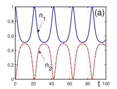
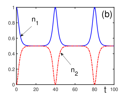
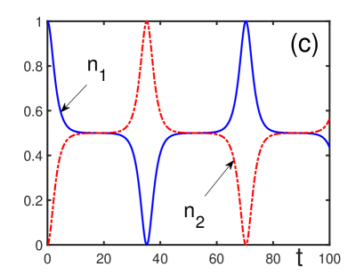
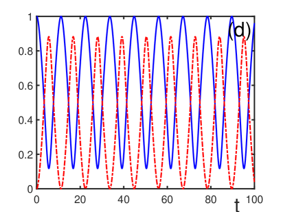
Figure 1: The time dependence of the fractional populations $n_{1}(t)$ (solid line) and $n_{2}(t)$ (dashed-dotted line) for $b=0.4999$ and (a) $\delta=0$; (b) flattening of the fractional populations with oscillation period being doubled for $\delta=0.0001$; (c) appearance of the upward cusps of $n_{1}(t)$ and downward cusps of $n_{2}(t)$ for $\delta=0.0001001$; (d) Regular oscillations for $\delta=0.3$.

The qualitative change of the phase portrait is called dynamical phase transition. In the vicinity of the dynamic critical line, there appear critical phenomena that are analogous to thermodynamic phase transitions. This can be shown by averaging the considered dynamical system over time [41, 75, 76].

The possibility of preserving resonance conditions is limited in time by a value of order

$$t_{res}~{}\sim~{}\frac{\omega_{21}}{\alpha^{2}+|\;\beta_{12}\;|^{2}}$$ (71)

that can be called resonance time [42]. After this time, the effect of power broadening comes into play, when other energy levels become involved, so that good resonance cannot be anymore supported. This limiting resonance time, in realistic trapping experiments, is of order of $10$ seconds, which is comparable to the lifetime of atoms in a trap [6, 78, 79].

9 Shape-conservation criterion

In order to transfer trapped atoms into an excited coherent mode, it is necessary to apply an alternating field. However not any, even resonant, field can generate a coherent mode. Some types of fields, would merely move the trapped atomic cloud without generating excited modes. The situation when the cloud does not change its shape, hence when no coherent modes are generated, despite the action of an alternating field, is described by the following theorem [80].

Theorem. Let atoms be trapped in a potential $U({\bf r})$, so that their state satisfies the trapping condition

$$\lim_{r\rightarrow\infty}\;\varphi({\bf r},t)~{}=~{}0\;.$$ (72)

And let these atoms, being at the initial moment of time in a real state $\varphi_{0}({\bf r})=\varphi_{0}^{*}({\bf r})$, be subjected to the action of an alternating field $V({\bf r},t)$. Then the solution to the nonlinear Schrödinger equation (15) satisfies the shape-conservation condition

$$|\;\varphi({\bf r},t)\;|~{}=~{}|\;\varphi({\bf r}-{\bf a}(t),0)\;|\;,$$ (73)

where $a(t)$ is a function of time, if and only if the trapping potential is harmonic,

$$U({\bf r})~{}=~{}A_{0}+{\bf A}_{1}{\bf r}+\sum_{\alpha\beta}A_{\alpha\beta}\;r^{\alpha}\;r^{\beta}\;,$$ (74)

and the alternating field is linear with respect to the spatial variables,

$$V({\bf r},t)=B_{0}(t)+{\bf B}_{1}(t)\cdot{\bf r}\;,$$ (75)

with $B_{0}(t)$ and ${\bf B}_{1}(t)$ being arbitrary functions of time.

In order to efficiently excite nonlinear coherent modes, it is required that at least one of the conditions (72) to (75) be invalid.

10 Multiple mode generation

It is feasible to generate not just a single coherent mode, but several of them. For this purpose, one needs to invoke an alternating field with several frequencies that are in resonance with the related transition frequencies. Generally, a multimode alternating field can be written in the form

$$V({\bf r},t)~{}=~{}\frac{1}{2}\sum_{j}\left[\;B_{j}({\bf r})e^{i\omega_{j}t}+B_{j}^{*}({\bf r})e^{-i\omega_{j}t}\;\right]\;,$$ (76)

with the modulation frequencies $\omega_{j}$ tuned to some transition frequencies $\omega_{mn}$. For example, the excitation of two coherent modes can be realized using one of three schemes that, similar to the optical excitation schemes [50], can be called cascade, $V$-type and $\Lambda$-type.

In the cascade scheme, one couples the first (ground-state) level with the second energy level and the second, with the third level by employing the alternating-field frequencies in resonance with the related energy differences:

$$\omega_{1}~{}=~{}\omega_{21}\;,\qquad\omega_{2}~{}=~{}\omega_{32}\qquad(cascade).$$ (77)

Here exact resonance conditions are defined. Generally, there can exist small detunings from the resonance.

In the $V$-type scheme, two alternating-field frequencies induce resonance with the transition frequencies, so that

$$\omega_{1}~{}=~{}\omega_{21}\;,\qquad\omega_{2}~{}=~{}\omega_{31}\qquad(V-type).$$ (78)

And in the $\Lambda$-type scheme, the coupling of the energy levels is realized by means of the resonance

$$\omega_{1}~{}=~{}\omega_{31}\;,\qquad\omega_{2}~{}=~{}\omega_{32}\qquad(\Lambda-type).$$ (79)

As in the case of two coherent modes, the solution to equation (15) is represented as the expansion

$$\varphi({\bf r},t)~{}=~{}\sum_{n}c_{n}(t)\;\varphi_{n}({\bf r})\;e^{-iE_{n}t}\;.$$ (80)

Then, following the same way as for two modes, we obtain the equations

$$i\;\frac{dc_{1}(t)}{dt}~{}=~{}\left(\alpha_{12}|\;c_{2}\;|^{2}+\alpha_{13}|\;c_{3}\;|^{2}\right)\;c_{1}+f_{1}\;,$$

$$i\;\frac{dc_{2}(t)}{dt}~{}=~{}\left(\alpha_{21}|\;c_{1}\;|^{2}+\alpha_{23}|\;c_{3}\;|^{2}\right)\;c_{2}+f_{2}\;,$$

$$i\;\frac{dc_{3}(t)}{dt}~{}=~{}\left(\alpha_{31}|\;c_{1}\;|^{2}+\alpha_{32}|\;c_{2}\;|^{2}\right)\;c_{3}+f_{3}\;,$$ (81)

in which the functions $f_{j}$ depend on the type of the generation scheme. The related detunings $\Delta\omega_{mn}$ from the resonance are assumed to be small

$$\left|\;\frac{\Delta\omega_{mn}}{\omega_{mn}}\;\right|~{}\ll~{}1\;,\qquad(\Delta\omega_{mn}\equiv\omega_{j}-\omega_{mn})\;.$$ (82)

For an example of the functions $f_{j}$, let us write down them for the cascade generation:

$$f_{1}~{}=~{}\frac{1}{2}\;\beta_{12}\;c_{2}\;e^{i\Delta\omega_{21}t}\;,$$

$$f_{2}~{}=~{}\frac{1}{2}\;\beta_{12}^{*}\;c_{1}\;e^{-i\Delta\omega_{21}t}+\frac{1}{2}\;\beta_{23}\;c_{3}\;e^{i\Delta\omega_{32}t}\;,$$

$$f_{3}~{}=~{}\frac{1}{2}\;\beta_{23}^{*}\;c_{2}\;e^{-i\Delta\omega_{32}t},$$ (83)

where

$$\Delta\omega_{21}~{}\equiv~{}\omega_{1}-\omega_{21}\;,\qquad\Delta\omega_{32}~{}\equiv~{}\omega_{2}-\omega_{32}\;.$$

The number of modes that could be excited is defined by the available number of states bound inside the trapping potential. For an infinitely rising potential, there is infinite number of state. Of course, in real experiments, trapping potentials are finite, hence they possess a finite number of states [81].

Solutions in the case of three modes have been analyzed in Refs. [80, 82, 83] using two ways, resorting to the averaging techniques [51] and by direct numerical solution of the nonlinear Schrödinger equation (15). Both ways were found to agree well with each other.

In the case of two coexisting nonlinear modes, the system of two complex differential equations (32), taking account of the normalization condition (30), has been reduced to two real differential equations (58). A two-dimensional dynamical system cannot exhibit chaotic motion. In our case, the fixed points where either centers or saddles.

For the case of three nonlinear modes, three complex equations (81) can be reduced to the system of four real differential equations. For this purpose, we introduce the real-valued phases $\zeta_{n}(t)$ by the representation

$$c_{n}~{}\equiv~{}|\;c_{n}\;|\;\exp(i\zeta_{n})\;.$$ (84)

We also use the notation

$$\beta_{mn}~{}=~{}b_{mn}\;\exp(i\gamma_{mn})\;,\qquad b_{mn}~{}\equiv~{}|\;\beta_{mn}\;|\;.$$ (85)

Introduce the population differences

$$s~{}\equiv~{}|\;c_{2}\;|^{2}-|\;c_{1}\;|^{2}\;,\qquad p~{}\equiv~{}|\;c_{3}\;|^{2}-|\;c_{2}\;|^{2}\;,$$ (86)

and the relative phases

$$x~{}\equiv~{}\zeta_{2}-\zeta_{1}+\gamma_{12}+\Delta\omega_{21}t\;,\qquad y~{}\equiv~{}\zeta_{3}-\zeta_{2}+\gamma_{23}+\Delta\omega_{32}t\;.$$ (87)

Then the mode populations can be written as

$$|\;c_{1}\;|^{2}~{}=~{}\frac{1}{3}\;(1-2s-p)\;,$$

$$|\;c_{2}\;|^{2}~{}=~{}\frac{1}{3}\;(1+s-p)\;,\qquad|\;c_{3}\;|^{2}~{}=~{}\frac{1}{3}\;(1+s+2p)\;.$$ (88)

Using these expressions makes it possible to reduce the system of six real equations (81) to the system of four equations. For instance, in the case of the cascade generation, we get

$$\frac{ds}{dt}~{}=~{}\frac{1}{3}\;\sqrt{1+s-p}\;(\;b_{23}\;\sqrt{1+s+2p}\;\sin y-2b_{12}\;\sqrt{1-2s-p}\;\sin x\;)\;,$$

$$\frac{dp}{dt}~{}=~{}\frac{1}{3}\;\sqrt{1+s-p}\;(\;b_{12}\;\sqrt{1-2s-p}\;\sin x-2b_{23}\;\sqrt{1+s+2p}\;\sin y\;)\;,$$

$$\frac{dx}{dt}~{}=~{}\alpha_{1}\;s+\delta_{1}\;p+\frac{3b_{12}s\cos x}{2\sqrt{(1+s-p)(1-2s-p)}}\;-\;\frac{1}{2}\;b_{23}\;\sqrt{\frac{1+s+2p}{1+s-p}}\;\cos y+\delta_{2}\;,$$

$$\frac{dy}{dt}~{}=~{}\alpha_{2}\;p+\delta_{3}\;s+\frac{3b_{23}p\cos y}{2\sqrt{(1+s-p)(1+s+2p)}}+\frac{1}{2}\;b_{12}\;\sqrt{\frac{1-2s-p}{1+s-p}}\;\cos x+\delta_{4}\;,$$ (89)

where

$$\alpha_{1}~{}\equiv~{}\frac{1}{3}\;(\alpha_{12}+\alpha_{13}+2\alpha_{21}-\alpha_{23})\;,\qquad\alpha_{2}~{}\equiv~{}\frac{1}{3}\;(\alpha_{32}+\alpha_{31}+2\alpha_{23}-\alpha_{21})\;,$$

$$\delta_{1}~{}\equiv~{}\frac{1}{3}\;(\alpha_{21}-\alpha_{12}+2\alpha_{13}-2\alpha_{23})\;,\qquad\delta_{2}~{}\equiv~{}\Delta\omega_{21}+\frac{1}{3}\;(\alpha_{12}-\alpha_{21}+\alpha_{13}-\alpha_{23})\;,$$

$$\delta_{3}~{}\equiv~{}\frac{1}{3}\;(\alpha_{23}-\alpha_{32}+2\alpha_{31}-2\alpha_{21})\;,\qquad\delta_{4}~{}\equiv~{}\Delta\omega_{32}+\frac{1}{3}\;(\alpha_{23}-\alpha_{32}+\alpha_{21}-\alpha_{31})\;.$$

The four-dimensional dynamical system (89) demonstrates the effects similar to those of the two-dimensional system (58), such as mode locking for small pumping amplitudes $b_{ij}$, however with quasi-periodic motion, instead of periodic Rabi oscillations. For large pumping amplitudes $b_{ij}$, there appears chaotic motion. For example, in the case where $\alpha_{mn}=\alpha$, $\beta_{mn}=\beta$, and $\Delta\omega_{mn}=0$, the chaotic motion arises when

$$\left|\;\frac{\beta}{\alpha}\;\right|~{}\geq~{}0.639448\;.$$

Note that here we consider cold bosonic atoms trapped in a potential that is not periodic, although similar effects can be generated in nonequilibrium optical latices as well [84, 85, 86, 87, 88, 89, 90, 91, 92, 93, 94, 95].

11 Matter-wave interferometry

Composing a coherent system, Bose condensates enjoy many of the properties typical of coherent optical systems and studied in atom interferometry [96]. In atoms, electrons can be excited into a higher individual energy level, while in a condensate a large group of trapped Bose-condensed atoms can be transferred into an excited collective energy level. The principal difference in dealing with many atoms, instead of a single atom, is in the necessity of taking account of interactions of condensed atoms.

11.1 Interference patterns

The existence of different coherent modes inside a trap leads to the appearance of interference patterns [42]. The density of atoms in a trap is

$$\rho({\bf r},t)~{}=~{}|\;\eta({\bf r},t)\;|^{2}~{}=~{}N\;|\;\varphi({\bf r},t)\;|^{2}\;.$$ (90)

With expression (20), this gives

$$\rho({\bf r},t)~{}=~{}N\left|\;\sum_{n}c_{n}(t)\;e^{-iE_{n}t}\;\varphi_{n}({\bf r})\;\right|^{2}\;.$$ (91)

The density of an $n$-th coherent mode is

$$\rho_{n}({\bf r},t)~{}=~{}N\;|\;c_{n}(t)\;\varphi_{n}({\bf r})\;|^{2}\;.$$ (92)

Therefore the interference pattern

$$\rho_{int}({\bf r},t)~{}\equiv~{}\rho({\bf r},t)-\sum_{n}\rho_{n}({\bf r},t)$$ (93)

reads as

$$\rho_{int}({\bf r},t)~{}=~{}N\sum_{m\neq n}c_{m}^{*}(t)\;c_{n}(t)\;\varphi_{m}^{*}({\bf r})\;\varphi_{n}({\bf r})\;e^{i\omega_{mn}t}.$$ (94)

Since the density of atoms can be observed, the interference pattern is also observable.

11.2 Internal Josephson current

The appearance of several coherent modes inside a trap makes the trapped atomic cloud essentially nonuniform, since different modes have different topological shapes. Respectively, inside the trap there arise a density current that is analogous to the current occurring between different potential wells [97, 98]. The current appearing not because of external barriers, but as a consequence of internally arising nonuniformities, is called internal Josephson current [99, 100]. This effect is also named quantum dynamical tunneling [101, 102].

The density current in a condensed system reads as

$${\bf j}({\bf r},t)~{}\equiv~{}\frac{1}{m}\;{\rm Im}\;\eta^{*}({\bf r},t)\;\vec{\nabla}\eta({\bf r},t)~{}=~{}\frac{N}{m}\;{\rm Im}\;\varphi^{*}({\bf r},t)\;\vec{\nabla}\varphi({\bf r},t)\;.$$ (95)

The current caused by a single mode is

$${\bf j}_{n}({\bf r},t)~{}=~{}\frac{N}{m}\;{\rm Im}\;|\;c_{n}(t)\;|^{2}\;\varphi_{n}^{*}({\bf r},t)\;\vec{\nabla}\varphi_{n}({\bf r},t)\;.$$ (96)

The difference between the total current in the system and the sum of density currents of separate modes forms the internal Josephson current [42]

$${\bf j}_{int}({\bf r},t)~{}=~{}\frac{N}{m}\;{\rm Im}\sum_{m\neq n}c_{m}^{*}(t)\;c_{n}(t)\;e^{i\omega_{mn}t}\;\varphi_{m}({\bf r},t)\;\vec{\nabla}\varphi_{n}({\bf r},t)\;.$$ (97)

11.3 Rabi oscillations

Under the action of an external alternating field, the mode fractional populations oscillate with time as in the case of Rabi oscillations [103]. Thus for two modes described by equations (32) the mode populations satisfy the equations

$$\frac{dn_{1}}{dt}~{}=~{}{\rm Im}\;\left(\beta_{12}\;e^{it\Delta\omega}\;c_{1}^{*}c_{2}\right)\;,\qquad\frac{dn_{2}}{dt}~{}=~{}{\rm Im}\;\left(\beta_{12}^{*}\;e^{-it\Delta\omega}\;c_{2}^{*}c_{1}\right)\;.$$ (98)

When $|\beta_{12}/\alpha|\ll 1$, then the amplitudes $c_{n}$ can be treated as fast functions, while $n_{1}$ and $n_{2}$, as slow. Then, employing the averaging method, under the initial conditions

$$c_{1}(0)~{}=~{}1\;,\qquad c_{2}(0)~{}=~{}0\;,$$ (99)

we find [22, 42] the guiding centers for the populations as

$$n_{1}~{}=~{}1\;-\;\frac{|\;\beta_{12}\;|^{2}}{\Omega^{2}}\;\sin^{2}\left(\frac{\Omega t}{2}\right)\;,\qquad n_{2}~{}=~{}\frac{|\;\beta_{12}\;|^{2}}{\Omega^{2}}\;\sin^{2}\left(\frac{\Omega t}{2}\right)\;,$$ (100)

with the effective Rabi frequency

$$\Omega^{2}=[\;\Delta\omega+\alpha\;(n_{2}-n_{1})\;]^{2}+|\;\beta_{12}\;|^{2}\;,$$ (101)

where, for simplicity, it is assumed that $\alpha_{12}=\alpha_{21}\equiv\alpha$. The Rabi oscillations can be used for studying the parameters of a two-level system.

11.4 Higher-order resonances

In addition to the resonance condition $\omega=\omega_{21}$, the generation of coherent modes can also be realized at higher-order resonances, under the effects of harmonic generation, employing a single external pumping field, with

$$n\omega~{}=~{}\omega_{21}\qquad(n=1,2,\ldots)\;,$$

and at parametric conversion, when several fields $\omega_{j}$ are used, such that

$$\sum_{j}(\pm\omega_{j})~{}=~{}\omega_{21}\;.$$

This can be shown [80, 82] by solving Eqs. (32) using the scale-separation approach [104, 105].

12 Ramsey fringes

Ramsey [106] improved upon Rabi’s method by splitting one interaction zone into two short interaction zones of time $\tau$, by applying two consecutive pulses separated by a long time interval $T\gg\tau$. The idea is to study the population $n_{2}$ of the excited atoms as a function of detuning or of separation time. In the case of coherent modes, the population $n_{2}$ describes the fraction of atoms in an excited collective coherent mode.

For a two-mode situation, equations (32) cannot be solved exactly because of the nonlinearity caused by atomic interactions. However, when $|\beta_{12}/\alpha|\ll 1$, it is possible to use averaging techniques, since then $c_{n}$ is classified as fast, while $n_{1}$ and $n_{2}$, as slow. Then equations (32) can be solved keeping the populations as quasi-integrals of motion. These equations can be rewritten [22] as

$$\frac{d^{2}c_{1}}{dt^{2}}\;-\;i(\Delta\omega-\alpha)\;\frac{dc_{1}}{dt}+\left[\;\frac{|\;\beta_{12}\;|^{2}}{4}+\alpha_{12}n_{2}\;(\Delta\omega-\alpha_{21}n_{1})\;\right]\;c_{1}~{}=~{}0\;,$$

$$\frac{d^{2}c_{2}}{dt^{2}}+i(\Delta\omega+\alpha)\;\frac{dc_{2}}{dt}+\left[\;\frac{|\;\beta_{12}\;|^{2}}{4}-\alpha_{21}n_{1}\;(\Delta\omega+\alpha_{12}n_{2})\;\right]\;c_{2}~{}=~{}0\;.$$ (102)

Introducing the notation for an effective detuning

$$\Delta~{}\equiv~{}\Delta\omega+\alpha_{12}n_{2}-\alpha_{21}n_{1}$$ (103)

and for an average interaction parameter

$$\alpha~{}\equiv~{}\alpha_{12}n_{2}+\alpha_{21}n_{1}\;,$$ (104)

we find the solutions of these equations

$$c_{1}(t)~{}=~{}\left\{\;c_{1}(0)\;\left[\;\cos\left(\frac{\Omega t}{2}\right)-i\;\frac{\Delta}{\Omega}\;\sin\left(\frac{\Omega t}{2}\right)\;\right]\;-\right.$$

$$\left.-\;i\;\frac{\beta_{12}}{\Omega}\;c_{2}(0)\sin\left(\frac{\Omega t}{2}\right)\;\right\}\;\exp\left\{\;\frac{i}{2}\;(\Delta\omega-\alpha)\;t\;\right\}\;,$$

$$c_{2}(t)~{}=~{}\left\{\;c_{2}(0)\;\left[\;\cos\left(\frac{\Omega t}{2}\right)-i\;\frac{\Delta}{\Omega}\;\sin\left(\frac{\Omega t}{2}\right)\;\right]\;-\right.$$

$$-\;\left.i\;\frac{\beta_{12}^{*}}{\Omega}\;c_{1}(0)\sin\left(\frac{\Omega t}{2}\right)\;\right\}\;\exp\left\{\;-\;\frac{i}{2}\;(\Delta\omega+\alpha)\;t\;\right\}\;.$$ (105)

If the first pulse acts during the time interval $0\leq t\leq\tau$ then at the end of the pulse, starting from the initial conditions (99), the solutions are

$$c_{1}(\tau)~{}=~{}\left[\;\cos\left(\frac{\Omega\tau}{2}\right)-i\;\frac{\Delta}{\Omega}\;\sin\left(\frac{\Omega\tau}{2}\right)\;\right]\;\exp\left\{\;\frac{i}{2}\;(\Delta\omega-\alpha)\tau\;\right\}\;,$$

$$c_{2}(\tau)~{}=~{}-i\;\frac{\beta_{12}^{*}}{\Omega}\;\sin\left(\frac{\Omega\tau}{2}\right)\;\exp\left\{\;-\;\frac{i}{2}\;(\Delta\omega+\alpha)\tau\;\right\}\;.$$ (106)

Then, during the time interval $\tau\leq t\leq t+T$, the external pulses are absent, which implies zero $\beta_{12}$. In that interval, the solutions have the form (105), where the initial conditions $c_{n}(0)$ are replaced by $c_{n}(\tau)$ from (106). Then, at time $\tau+T$, we have

$$c_{1}(\tau+T)~{}=~{}c_{1}(\tau)\;\left[\;\cos\left(\frac{\Omega(\tau+T)}{2}\right)-i\;\frac{\Delta}{\Omega}\;\sin\left(\frac{\Omega(\tau+T)}{2}\right)\;\right]\;\times$$

$$\times\;\exp\left\{\;\frac{i}{2}\;(\Delta\omega-\alpha)(\tau+T)\;\right\}\;,$$

$$c_{2}(\tau+T)~{}=~{}c_{2}(\tau)\;\left[\;\cos\left(\frac{\Omega(\tau+T)}{2}\right)-i\;\frac{\Delta}{\Omega}\;\sin\left(\frac{\Omega(\tau+T)}{2}\right)\;\right]\;\times$$

$$\times\;\exp\left\{\;-\;\frac{i}{2}\;(\Delta\omega+\alpha)(\tau+T)\;\right\}\;.$$ (107)

Following this way, at the end of the second pulse we find the amplitude of the excited mode

$$c_{2}(2\tau+T)~{}=~{}-i\;\frac{\beta_{12}^{*}}{\Omega}\;\sin\left(\frac{\Omega\tau}{2}\right)\;\times$$

$$\times\;\left\{\;\left[\;\cos\left(\frac{\Omega\tau}{2}\right)-i\;\frac{\Delta}{\Omega}\;\sin\left(\frac{\Omega\tau}{2}\right)\;\right]\;\exp\left[\;-i(\Delta\omega+\alpha_{12}n_{2})\;T\;\right]\right.\;+$$

$$+\;\left.\left[\;\cos\left(\frac{\Omega\tau}{2}\right)+i\;\frac{\Delta}{\Omega}\;\sin\left(\frac{\Omega\tau}{2}\right)\;\right]\;\exp(-i\alpha_{21}n_{1}\tau)\;\right\}\;\exp\{-i(\Delta\omega+\alpha)\tau\}\;.$$ (108)

Therefore, the related population difference $n_{2}=|c_{2}|^{2}$ reads as

$$n_{2}(2\tau+T)~{}=~{}4\;\frac{|\;\beta_{12}\;|^{2}}{\Omega^{2}}\;\sin^{2}\left(\frac{\Omega\tau}{2}\right)\;\times$$

$$\times\;\left[\;\cos\left(\frac{\Omega\tau}{2}\right)\;\cos\left(\frac{\Delta T}{2}\right)+\frac{\Delta}{\Omega}\;\sin\left(\frac{\Omega\tau}{2}\right)\;\sin\left(\frac{\Delta T}{2}\right)\;\right]^{2}.$$ (109)

Usually, one works with the so-called $\pi/2$ pulses, when $\Omega\tau=\pi/2$. Then

$$n_{2}(2\tau+T)~{}=~{}\frac{|\;\beta_{12}\;|^{2}}{\Omega^{2}}\;\left[\;\cos\left(\frac{\Omega\tau}{2}\right)+\frac{\Delta}{\Omega}\;\sin\left(\frac{\Delta T}{2}\right)\;\right]^{2}\;.$$ (110)

The excited mode population is studied as a function of the detuning $\Delta\omega$. The corresponding oscillating function $n_{2}$, demonstrating Ramsey fringes, is shown in Refs. [107, 108]. The Ramsey fringes, caused by coherent modes, are similar to Ramsey fringes of binary Bose condensate mixtures of two different components [109] or of mixtures with two different internal states [110], or of mixtures consisting of atoms and molecules [111].

13 Interaction modulation

The atomic scattering length can be varied in the presence of an external magnetic field $B$ due to Feshbach resonance [112]. The magnetic field can be varied in time, $B=B(t)$. Then the related scattering length

$$a_{s}(B)~{}=~{}a_{s}\;\left(1\;-\;\frac{\Delta B}{B-B_{res}}\right)\;,$$ (111)

where $a_{s}$ is the scattering length far outside of the resonance field $B_{res}$ and $\Delta B$ is the resonance width, also becomes time dependent, as well as the interaction strength

$$\Phi(t)~{}=~{}4\pi\;\frac{a_{s}(B)}{m}\;,\qquad B~{}=~{}B(t)\;.$$ (112)

If the magnetic field $B(t)$ is modulated around a field $B_{0}$, so that

$$B(t)~{}=~{}B_{0}+b(t)\;,$$ (113)

with a small modulation amplitude $|b(t)/B_{0}|\ll 1$ oscillating as

$$b(t)~{}=~{}b_{1}\cos(\omega t)+b_{2}\sin(\omega t)\;,$$ (114)

then the effective interaction strength acquires the form

$$\Phi(t)~{}=~{}\Phi_{0}+\Phi_{1}\cos(\omega t)+\Phi_{2}\sin(\omega t)\;,$$ (115)

where

$$\Phi_{0}~{}=~{}\frac{4\pi}{m}\;a_{s}\left(1\;-\;\frac{\Delta B}{B_{0}-B_{res}}\right)\;,$$

$$\Phi_{1}~{}=~{}\frac{4\pi a_{s}b_{1}\Delta B}{m(B_{0}-B_{res})^{2}}\;,\qquad\Phi_{2}~{}=~{}\frac{4\pi a_{s}b_{2}\Delta B}{m(B_{0}-B_{res})^{2}}\;.$$

Resonance modulation of the effective interaction can generate coherent modes, similarly to the trap modulation, as has been mentioned in [113] and studied in [15, 114, 115].

Thus we are looking for the solution of the nonlinear Schrödinger equation

$$i\;\frac{\partial}{\partial t}\;\varphi({\bf r},t)~{}=~{}\hat{H}(t)\;\varphi({\bf r},t)\;,$$ (116)

with the effective time-dependent Hamiltonian

$$\hat{H}(t)~{}=~{}-\;\frac{\nabla^{2}}{2m}+U({\bf r})+N\;\Phi(t)\;|\;\varphi({\bf r},t)\;|^{2}\;.$$ (117)

Substituting here the mode expansion

$$\varphi({\bf r},t)~{}=~{}\sum_{n}c_{n}(t)\;e^{-iE_{n}t}\;\varphi_{n}({\bf r})\;,$$ (118)

keeping in mind the two-mode case, following the same procedure as above, and using the notation

$$\gamma_{1}~{}\equiv~{}(\Phi_{1}-i\Phi_{2})\;N\int\varphi_{1}^{*}({\bf r})|\;\varphi_{1}({\bf r},t)\;|^{2}\varphi_{2}({\bf r})\;d{\bf r}\;,$$

$$\gamma_{2}~{}\equiv~{}(\Phi_{1}-i\Phi_{2})\;N\int\varphi_{1}^{*}({\bf r})|\;\varphi_{2}({\bf r},t)\;|^{2}\varphi_{2}({\bf r})\;d{\bf r}\;,$$ (119)

we obtain the equations for the mode amplitudes

$$i\;\frac{dc_{1}}{dt}~{}=~{}\alpha_{12}|\;c_{2}\;|^{2}c_{1}+\left(\gamma_{1}\;|\;c_{1}\;|^{2}+\frac{1}{2}\;\gamma_{2}\;|\;c_{2}\;|^{2}\right)\;c_{2}e^{i\Delta\omega t}+\frac{1}{2}\;\gamma_{1}^{*}\;c_{2}^{*}\;c_{1}^{2}\;e^{-i\Delta\omega t}\;,$$

$$i\;\frac{dc_{2}}{dt}~{}=~{}\alpha_{21}|\;c_{1}\;|^{2}c_{2}+\left(\gamma_{2}^{*}\;|\;c_{2}\;|^{2}+\frac{1}{2}\;\gamma_{1}^{*}\;|\;c_{1}\;|^{2}\right)\;c_{1}e^{-i\Delta\omega t}+\frac{1}{2}\;\gamma_{2}\;c_{1}^{*}\;c_{2}^{2}\;e^{i\Delta\omega t}\;.$$ (120)

Generally, it is possible to combine the mode generation by means of trap modulation as well as by scattering length modulation. This can be used for generating multiple coherent modes or for enhancing the resonant generation of a special mode. Then, employing the same procedures as above, we derive [115] the equations

$$i\;\frac{dc_{1}}{dt}~{}=~{}\alpha_{12}|\;c_{2}\;|^{2}c_{1}+\frac{1}{2}\;\left(2\gamma_{1}\;|\;c_{1}\;|^{2}+\gamma_{2}\;|\;c_{2}\;|^{2}+\beta_{12}\right)\;c_{2}\;e^{i\Delta\omega t}+\frac{1}{2}\;\gamma_{1}^{*}\;c_{2}^{*}\;c_{1}^{2}\;e^{-i\Delta\omega t}\;,$$

$$i\;\frac{dc_{2}}{dt}~{}=~{}\alpha_{21}|\;c_{1}\;|^{2}c_{2}+\frac{1}{2}\;\left(2\gamma_{2}^{*}\;|\;c_{2}\;|^{2}+\gamma_{1}^{*}\;|\;c_{1}\;|^{2}+\beta_{12}^{*}\right)\;c_{1}\;e^{-i\Delta\omega t}+\frac{1}{2}\;\gamma_{2}\;c_{1}^{*}\;c_{2}^{2}\;e^{i\Delta\omega t}\;.$$ (121)

Equations (120) and (121) have the structure similar to Eqs. (32), hence they can produce the same effects involving coherent modes [15, 114, 115]. The generation of coherent modes can be effectively done by both methods, by means of external potential modulation or by modulating atomic interactions [15, 114, 115, 116, 117].

14 Strong interactions and noise

In the above sections, generation of coherent modes is treated in the regime of asymptotically weak interactions and in the absence of noise corresponding to temperature. The condensate wave equation (15) has been obtained assuming that all atoms are condensed. This has allowed us, for deriving the condensate wave-function equation, to resort to the coherent approximation, resulting in the nonlinear Schrödinger equation (15). Of course, at finite, and moreover under strong interactions, the condensate can be essentially depleted. In addition, there can exist intrinsic noise imitating temperature effects.

Thus, three questions arise. First, what is the wave-function equation for finite and strong atomic interactions? Second, is it feasible to generate coherent modes with that condensate equation? And, third, what is the influence of intrinsic noise on the mode dynamics? This section provides answers to these questions. Below, we follow the self-consistent theory of Bose-condensed systems [15, 16, 23, 118, 119, 120, 121].

When in a Bose system, described by the Hamiltonian (3), there occurs Bose-Einstein condensation, the global gauge symmetry becomes broken. The symmetry breaking is the necessary and sufficient condition for Bose condensation [12, 15]. The explicit and convenient way of symmetry breaking is by means of the Bogolubov shift

$$\psi({\bf r},t)~{}=~{}\eta({\bf r},t)+\psi_{1}({\bf r},t)\;,$$ (122)

where $\eta({\bf r},t)$ is the condensate wave function and $\psi_{1}({\bf r},t)$ is the field operator of uncondensed atoms. The field variables of condensed and uncondensed particles are mutually orthogonal,

$$\int\eta^{*}({\bf r},t)\;\psi_{1}({\bf r},t)\;d{\bf r}~{}=~{}0\;.$$ (123)

The condensate wave function is normalized to the number of condensed atoms

$$N_{0}~{}=~{}\int|\;\eta({\bf r},t)\;|^{2}\;d{\bf r}\;,$$ (124)

while the number of uncondensed atoms is

$$N_{1}~{}=~{}\int\langle\;\psi_{1}^{\dagger}({\bf r},t)\;\psi_{1}({\bf r},t)\;\rangle\;d{\bf r}\;.$$ (125)

The total number of atoms

$$N~{}=~{}N_{0}+N_{1}$$ (126)

is fixed.

In order that the quantum numbers, such as spin or momentum, be conserved, requires to impose the conservation condition

$$\langle\;\psi_{1}({\bf r},t)\;\rangle~{}=~{}0\;.$$ (127)

The general form of the conservation condition is written as

$$\langle\;\hat{\Lambda}\;\rangle~{}=~{}0\;,$$ (128)

with the condition operator

$$\hat{\Lambda}~{}=~{}\int\left[\;\lambda({\bf r},t)\;\psi_{1}^{\dagger}({\bf r},t)+\lambda^{*}({\bf r},t)\;\psi_{1}({\bf r},t)\;\right]\;d{\bf r}\;,$$ (129)

in which $\lambda({\bf r},t)$ is a Lagrange multiplier.

Taking into account the normalization conditions (124) and (125), as well as the conservation condition (128), leads to the grand Hamiltonian

$$H~{}=~{}\hat{H}-\mu_{0}N_{0}-\mu_{1}\hat{N}_{1}-\hat{\Lambda}\;,$$ (130)

where

$$\hat{N}_{1}~{}=~{}\int\psi_{1}^{\dagger}({\bf r},t)\;\psi_{1}({\bf r},t)\;d{\bf r}\;.$$ (131)

The evolution equations for condensed and uncondensed atoms are

$$i\;\frac{\partial}{\partial t}\;\eta({\bf r},t)~{}=~{}\left\langle\;\frac{\delta H}{\delta\eta^{*}({\bf r},t)}\;\right\rangle$$ (132)

and, respectively,

$$i\;\frac{\partial}{\partial t}\;\psi_{1}({\bf r},t)~{}=~{}\frac{\delta H}{\delta\psi_{1}^{\dagger}({\bf r},t)}\;.$$ (133)

The conservation condition (128) requires that the grand Hamiltonian must have no linear in $\psi_{1}$ terms, which is achieved by setting the Lagrange multiplier

$$\lambda({\bf r},t)~{}=~{}\left[\;-\;\frac{\nabla^{2}}{2m}+U({\bf r},t)+\frac{1}{2}\int\Phi({\bf r}-{\bf r}^{\prime})\;|\;\eta({\bf r}^{\prime},t)\;|^{2}\;d{\bf r}^{\prime}\;\right]\;\eta({\bf r},t)\;.$$ (134)

To proceed further, let us introduce several notations, such as the normal density matrix

$$\rho_{1}({\bf r},{\bf r}^{\prime},t)~{}\equiv~{}\langle\;\psi_{1}^{\dagger}({\bf r}^{\prime},t)\;\psi_{1}({\bf r},t)\;\rangle\;,$$ (135)

the so-called anomalous average

$$\sigma_{1}({\bf r},{\bf r}^{\prime},t)~{}\equiv~{}\langle\;\psi_{1}({\bf r}^{\prime},t)\;\psi_{1}({\bf r},t)\;\rangle\;,$$ (136)

the density of condensed atoms

$$\rho_{0}({\bf r},t)~{}\equiv~{}|\;\eta({\bf r},t)\;|^{2}\;,$$ (137)

the density of uncondensed atoms

$$\rho_{1}({\bf r},t)~{}\equiv~{}\langle\;\psi_{1}^{\dagger}({\bf r},t)\;\psi_{1}({\bf r},t)\;\rangle~{}=~{}\rho_{1}({\bf r},{\bf r},t)\;,$$ (138)

the total density of atoms

$$\rho({\bf r},t)~{}=~{}\rho_{0}({\bf r},t)+\rho_{1}({\bf r},t)\;,$$ (139)

the diagonal anomalous average

$$\sigma_{1}({\bf r},t)~{}\equiv~{}\langle\;\psi_{1}({\bf r},t)\;\psi_{1}({\bf r},t)\;\rangle~{}=~{}\sigma_{1}({\bf r},{\bf r},t)\;,$$ (140)

and the triple anomalous average

$$\xi({\bf r},{\bf r}^{\prime},t)~{}\equiv~{}\langle\;\psi_{1}^{\dagger}({\bf r}^{\prime},t)\;\psi_{1}({\bf r}^{\prime},t)\;\psi_{1}({\bf r},t)\;\rangle\;.$$ (141)

With these notations, the equation for the condensate wave function reads as

$$i\;\frac{\partial}{\partial t}\;\eta({\bf r},t)~{}=~{}\left[-\;\frac{\nabla^{2}}{2m}+U({\bf r},t)-\mu_{0}\;\right]\;\eta({\bf r},t)\;+$$

$$+\;\int\Phi({\bf r}-{\bf r}^{\prime})\;\left[\;\rho({\bf r}^{\prime},t)\;\eta({\bf r},t)+\rho_{1}({\bf r},{\bf r}^{\prime},t)\;\eta({\bf r}^{\prime},t)+\sigma({\bf r},{\bf r}^{\prime},t)\;\eta^{*}({\bf r}^{\prime},t)+\xi({\bf r},{\bf r}^{\prime},t)\;\right]\;d{\bf r}^{\prime}\;.$$ (142)

Note that this is an exact equation valid for any integrable interaction potential. For the contact potential (4), the equation takes the form

$$i\;\frac{\partial}{\partial t}\;\eta({\bf r},t)~{}=~{}\left[-\;\frac{\nabla^{2}}{2m}+U({\bf r},t)-\mu_{0}\;\right]\;\eta({\bf r},t)\;+$$

$$+\;\Phi_{0}\{\;[\;\rho_{0}({\bf r},t)+2\rho_{1}({\bf r},t)\;]\;\eta({\bf r},t)+\sigma_{1}({\bf r},t)\;\eta^{*}({\bf r},t)+\xi({\bf r},t)\;\}\;,$$ (143)

in which

$$\xi({\bf r},t)~{}\equiv~{}\xi({\bf r},{\bf r},t)\;.$$ (144)

The solution to this equation can be sought in the form

$$\eta({\bf r},t)~{}=~{}\sqrt{N_{0}(t)}\;\sum_{n}c_{n}(t)\;\varphi_{n}({\bf r})\;\exp\{-i[\;E_{n}+\varepsilon_{n}(t)-\mu_{0}\;]\;t\}\;.$$ (145)

If the number of condensed atoms changes slowly in time, so that

$$\left|\;\frac{1}{E_{n}}\;\frac{dN_{0}(t)}{dt}\;\right|~{}\ll~{}1$$ (146)

and the phase $\varepsilon_{n}(t)$ is also a slow function of time,

$$\left|\;\frac{1}{E_{n}}\;\frac{d\varepsilon_{n}(t)}{dt}\;\right|~{}\ll~{}1\;,$$ (147)

then, in the case of two coherent modes, we obtain [15, 119] the same equations (121). However, the phase $\varepsilon_{n}(t)$ is a slow function when $\rho_{1}$, $\sigma_{1}$, and $\xi$ are small as compared to $\rho_{0}$.

In this way, when interactions between atoms are strong and temperature is high, the phase of the condensate wave function can very rather fast. In order to understand how fast phase fluctuations influence the dynamics of the condensate wave function, it is possible to consider the equations

$$\frac{ds}{dt}~{}=~{}-\beta\;\sqrt{1-s^{2}}\;\sin x\;,$$

$$\frac{dx}{dt}~{}=~{}\alpha\;s+\frac{\beta s}{\sqrt{1-s^{2}}}\;\cos x+\delta+\sigma\;dW_{t}\;,$$ (148)

in which phase fluctuations are modeled by random noise, where $W_{t}$ is the standard Wiener process and $\sigma$ is the standard noise deviation. These equations are to be compared with equations (58) containing no random phase fluctuations. If the strength of the noise is not too large, its influence leads to the distortion of Rabi oscillations, but does not change the overall qualitative picture [122, 123], as is shown in Fig. 2 for the mode-locked (subcritical) regime) and Fig. 3 for the mode-unlocked (supercritical regime).

     

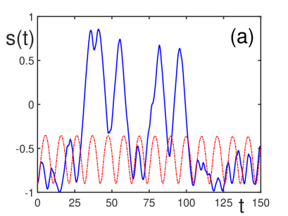
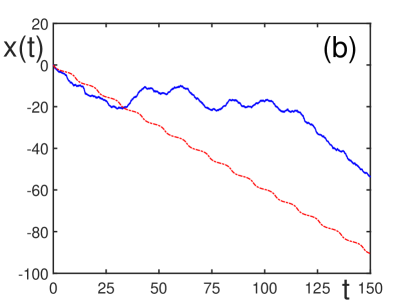
Figure 2: Subcritical regime with $b=0.25<b_{c}=0.282$. (a) Population imbalance s(t) as functions of dimensionless time, for $\sigma=0.5$ (solid line) and $\sigma=0$ (dashed-dotted line). (b) Phase difference x(t) as functions of dimensionless time, for $\sigma=0.5$ (solid line) and $\sigma=0$ (dashed-dotted line).

     

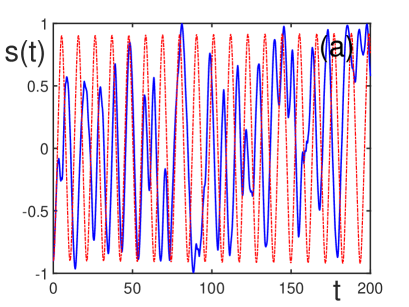
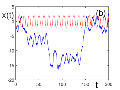
Figure 3: Supercritical regime with $b=0.5>b_{c}=0.282$. (a) Population imbalance s(t) as functions of dimensionless time, for $\sigma=0.5$ (solid line) and $\sigma=0$ (dashed-dotted line). (b) Phase difference x(t) as functions of dimensionless time, for $\sigma=0.5$ (solid line) and $\sigma=0$ (dashed-dotted line).

15 Critical phenomena

The qualitative change of dynamics between the mode-locked regime and mode-unlocked regime reminds a phase transition in a statistical system. This similarity can be emphasized by considering an effective stationary system obtained by averaging the original system over time [41, 75, 76, 77].

For simplicity, we set $\alpha_{12}=\alpha_{21}=\alpha$. In the case of two coherent modes, the evolution equations (32) can be derived from the Hamiltonian equations

$$i\;\frac{dc_{1}}{dt}~{}=~{}\frac{\partial H}{\partial c_{1}^{*}}\;,\qquad i\;\frac{dc_{2}}{dt}~{}=~{}\frac{\partial H}{\partial c_{2}^{*}}\;,$$ (149)

with the effective Hamiltonian

$$H~{}=~{}\alpha\;|\;c_{1}\;c_{2}\;|^{2}+\frac{1}{2}\;\left(\beta\;c_{1}^{*}\;c_{2}\;e^{i\Delta\omega t}+\beta^{*}\;c_{2}^{*}\;c_{1}\;e^{-i\Delta\omega t}\right)\;,$$ (150)

in which $\beta\equiv\beta_{12}$. Resorting to the averaging techniques yields solution (105).

Averaging Hamiltonian (150) over time, with using the normalization condition

$$n_{1}+n_{2}~{}=~{}1\;,$$ (151)

gives the effective energy

$$E~{}=~{}\frac{\alpha|\;\beta\;|^{2}}{2\overline{\Omega}^{2}}\;\left(\frac{|\;\beta\;|^{2}}{2\overline{\Omega}^{2}}+\varepsilon\right)\;,$$ (152)

with $\varepsilon\equiv\delta/\alpha$, the average Rabi frequency given by the expression

$$\overline{\Omega}^{2}~{}=~{}\alpha^{2}\;\left(\varepsilon+\overline{n}_{2}-\overline{n}_{1}\right)^{2}+|\;\beta\;|^{2}\;,$$ (153)

and the average fractions

$$\overline{n}_{1}~{}=~{}1-\overline{n}_{2}\;,\qquad\overline{n}_{2}~{}=~{}\frac{|\;\beta\;|^{2}}{2\overline{\Omega}^{2}}\;.$$ (154)

The order parameter can be defined as the average population difference

$$\eta~{}\equiv~{}\overline{n}_{1}-\overline{n}_{2}~{}=~{}1\;-\;\frac{|\;\beta\;|^{2}}{\overline{\Omega}^{2}}\;.$$ (155)

Also, let us introduce the system capacity to store the energy pumped into the system

$$C_{\beta}~{}\equiv~{}\frac{\partial E}{\partial|\;\beta\;|}$$ (156)

and the susceptibility with respect to detuning

$$\chi_{\varepsilon}~{}\equiv~{}\frac{\partial\eta}{\partial|\;\varepsilon\;|}\;.$$ (157)

The abrupt change of dynamics happens on the critical line $b_{c}+\varepsilon=0.5$, where $b\equiv\beta/\alpha$. In the vicinity of the dynamic phase transition, the system characteristics strongly depend on the variable

$$\tau~{}\equiv~{}\frac{|\;b-b_{c}\;|}{b_{c}}\;.$$ (158)

When $\tau\rightarrow 0$, we observe the critical behavior of the order parameter

$$\eta-\eta_{c}~{}\simeq~{}\frac{1}{\sqrt{2}}\;(1-2\varepsilon)\;\tau^{1/2}\qquad(\eta_{c}~{}=~{}0.5+\varepsilon)\;,$$ (159)

effective system capacity and susceptibility:

$$C_{\beta}~{}\simeq~{}\frac{1}{4\sqrt{2}}\;\tau^{-1/2}\;,\qquad\chi_{\varepsilon}~{}\simeq~{}\frac{1}{\sqrt{2}}\;\tau^{-1/2}\;.$$ (160)

The latter diverge as at phase transitions of second order.

The critical exponents of the order parameter, capacity, and susceptibility satisfy the scaling relation

$$\frac{1}{2}+1+\frac{1}{2}~{}=~{}2$$ (161)

typical of equilibrium second-order phase transitions.

16 Atomic squeezing

Bose-Einstein condensation is accompanied by global gauge symmetry breaking, when the arising condensate is characterized by a wave function. Rigorous description of the Bose-condensate assumes the thermodynamic limit. In a finite volume, strictly speaking, there is no Bose-condensate, but there exists a quasi-condensate that is described by field operators. Hence, a finite cloud of trapped atoms should be characterized by operators instead of non-operator functions. In order to consider a finite quasi-condensate, one has to replace the amplitudes $c_{n}$ by Bose operators ${\hat{c}}_{n}$.

When one is interested in the case of two modes, one can make the canonical transformation to quasi-spin operators

$$\hat{c}_{1}^{\dagger}\;\hat{c}_{1}~{}=~{}\frac{1}{2}\;-\;S_{z}\;,\qquad\hat{c}_{2}^{\dagger}\;\hat{c}_{2}~{}=~{}\frac{1}{2}\;+\;S_{z}\;,$$

$$\hat{c}_{1}^{\dagger}\;\hat{c}_{2}~{}=~{}S_{x}-iS_{y}\;,\qquad\hat{c}_{2}^{\dagger}\;\hat{c}_{1}~{}=~{}S_{x}+iS_{y}\;,$$ (162)

where

$$S_{\alpha}~{}\equiv\sum_{j=1}^{N}S_{j}^{\alpha}\qquad(\alpha=x,y,z)\;.$$

The evolution equations can be derived [42] using the standard Heisenberg equations of motion with the Hamiltonian

$$H~{}=~{}-\;\frac{\alpha}{N}\;S_{z}^{2}+\frac{\beta}{2}\;(S^{-}+S^{+})-S_{z}\;\delta\;,$$ (163)

in which $S_{j}^{\alpha}$ are half-spin operators and the ladder operators are

$$S^{\pm}~{}\equiv~{}S_{x}\pm iS_{y}\;.$$

Averaging these equations, with employing the mean-field approximation, gives equations equivalent to Eqs. (58).

Then it is possible to study the problem of squeezing in trapped atomic systems, similarly to the squeezing of light in optical systems [50]. In general, atomic squeezing can be achieved for both bosons as well as for fermions. Squeezing for Bose-Einstein condensates was considered for two-component mixtures [124], for atoms with two internal states [125], and for atoms in linked mesoscopic traps formed by an optical lattice [126], which is equivalent to a multicomponent mixture. Atomic squeezing can be used for atomic spectroscopy, creation of atomic clocks [127], and for atom interferometers [128].

For any two operators, $\hat{A}$ and $\hat{B}$, there exists the Heisenberg uncertainty relation

$${\rm var}(\hat{A})\;{\rm var}(\hat{B})~{}\geq~{}\frac{1}{4}\;\left|\;\langle\;[\;\hat{A},\;\hat{B}\;]\;\rangle\;\right|^{2}\;,$$ (164)

where the variance is

$${\rm var}(\hat{A})~{}\equiv~{}\langle\;\hat{A}^{+}\;\hat{A}\;\rangle-|\;\langle\;\hat{A}\;\rangle\;|^{2}\;.$$

One says that the operators $\hat{A}$ and $\hat{B}$ are not squeezed with respect to each other, when

$$\begin{array}[]{l}{\rm var}(\hat{A})~{}\geq~{}\frac{1}{2}\;|\;\langle\;[\;\hat{A},\;\hat{B}\;]\;\rangle\;|\\ {\rm var}(\hat{B})~{}\geq~{}\frac{1}{2}\;|\;\langle\;[\;\hat{A},\;\hat{B}\;]\;\rangle\;|\end{array}~{}~{}~{}(not\;squeezed)\;.$$ (167)

And one says that $\hat{A}$ is squeezed with respect to $\hat{B}$, if

$${\rm var}(\hat{A})~{}<~{}\frac{1}{2}\;\left|\;\langle\;[\;\hat{A},\;\hat{B}\;]\;\rangle\;\right|\qquad(squeezed)\;.$$ (168)

The measure of squeezing is quantified by the squeezing factor

$$Q_{AB}~{}\equiv~{}\frac{2{\rm var}(\hat{A})}{|\;\langle\;[\;\hat{A},\;\hat{B}\;]\;\rangle\;|}\;.$$ (169)

For two operators, squeezing happens when the squeezing factor is smaller than unity,

$$\begin{array}[]{ll}Q_{AB}~{}\geq~{}1{}{}&~{}~{}(no\;squeezing)\;,\\ Q_{AB}~{}<~{}1{}{}&~{}~{}(squeezing)\;.\end{array}$$ (172)

The occurrence of squeezing of $\hat{A}$ with respect to $\hat{B}$ implies that the observable corresponding to $\hat{A}$ can be measured more precisely than that one related to $\hat{B}$.

In our case, the operator $S_{z}$ corresponds to the population difference, while $S^{\pm}$, to the transition dipoles, since

$$\langle\;S_{z}\;\rangle~{}=~{}\frac{N}{2}\;s\;,\qquad|\;\langle\;S^{\pm}\;\rangle\;|~{}=~{}\frac{N}{2}\;|\;\langle\;\hat{c}_{1}^{\dagger}\;\hat{c}_{2}\;\rangle\;|\;.$$ (173)

For the related operators, the Heisenberg uncertainty relation is

$${\rm var}(S_{z})\;{\rm var}(S^{\pm})~{}\geq~{}\frac{1}{4}|\;\langle\;S^{\pm}\;\rangle\;|^{2}\;.$$ (174)

Squeezing of $S_{z}$ with respect to $S^{\pm}$ is measured by the squeezing factor

$$Q~{}=~{}\frac{2{\rm var}(S_{z})}{|\;\langle\;S^{\pm}\;\rangle\;|}\;,$$ (175)

which leads to

$$Q~{}=~{}\sqrt{1-s^{2}}\;.$$ (176)

In the mode-locked regime, $s^{2}\leq 1$, and $Q<1$ for all times. In the mode-unlocked regime $s^{2}$ for the most of time is smaller than one, touching one only at some moments of time. Hence almost always $S_{z}$ is squeezed with respect to $S^{\pm}$. This means that the population difference, hence the mode populations, can be measured with a better accuracy than the quantities associated with the transition dipoles, such as density current.

Similarly, it is possible to consider the effect of squeezing for several coupled modes. Thus, for three modes, it is straightforward to introduce the quasi-spin operators

$$J_{+}~{}\equiv~{}\sqrt{2}\;(a_{2}^{\dagger}\;a_{1}+a_{3}^{\dagger}\;a_{2})\;,\qquad J_{-}~{}\equiv~{}\sqrt{2}\;(a_{1}^{\dagger}\;a_{2}+a_{2}^{\dagger}\;a_{3})\;,\qquad J_{z}~{}\equiv~{}a_{3}^{\dagger}\;a_{3}-a_{1}^{\dagger}\;a_{1}\;,$$

satisfying the commutation relations

$$[\;J_{+},\;J_{-}\;]~{}=~{}2J_{z}\;,\qquad[\;J_{z},\;J_{\pm}\;]~{}=~{}\pm J_{\pm}\;.$$

Then the squeezing factor is defined in the same way as for two modes.

17 Cloud entanglement

It is necessary to distinguish two different notions, entanglement of states and entanglement production. Entanglement of a state concerns the structure of a statistical operator, while entanglement production by an operator describes the ability of an operator, by acting on functions of a Hilbert space, to create entangled functions.

17.1 Entangled states

When one talks about entanglement, one has, first of all, to specify what are the objects whose entanglement is considered. In quantum physics it is customary to consider entanglement of particles. However in the case of Bose-Einstein condensate, it is possible to study entanglement between large atomic clouds. Such coherent atomic clouds can be organized in optical lattices with sufficiently deep wells at lattice sites. Each lattice well can house condensate clouds containing between several atoms to $10^{4}$ atoms [129, 130]. Shaking the optical lattice by means of magnetic fields or lasers, it is possible to excite coherent modes simultaneously in all lattice sites.

Suppose Bose-condensed atoms are loaded into a deep lattice with $N_{L}$ sites, enumerated by the index $j=1,2,\ldots,N_{L}$, where at each lattice site there is a cloud of $N$ atoms, with $N\gg 1$. Assume that there can be excited $M$ coherent modes enumerated by the index $m=1,2,\ldots,M$. A coherent mode $m$ at a lattice site $j$, which is characterized by a coherent field $\eta_{jm}({\bf r})$, in the Fock space is represented [131] by a column

$$|\;\eta_{jm}\;\rangle~{}=~{}\left[\;\frac{e^{-N/2}}{\sqrt{n!}}\;\prod_{i=1}^{n}\eta_{jm}({\bf r}_{i})\;\right]\;,$$ (177)

with the rows enumerated by $n=0,1,2,\ldots$. These modes form a basis in the space

$${\cal H}_{j}~{}=~{}{\rm span}_{m}\{\;|\;\eta_{jm}\;\rangle\;\}\;.$$ (178)

The overall system of $N_{L}$ clouds is described by the Hilbert space

$${\cal H}~{}=~{}\bigotimes_{j=1}^{N_{L}}{\cal H}_{j}~{}=~{}{\rm span}_{m}\left\{\bigotimes_{j=1}^{N_{L}}|\;\eta_{jm}\;\rangle\;\right\}\;.$$ (179)

The coherent wave state of the whole system in the Fock space is

$$|\;\eta(t)\;\rangle~{}=~{}\sum_{m=1}^{M}c_{m}(t)\bigotimes_{j=1}^{N_{L}}|\;\eta_{jm}\;\rangle\;.$$ (180)

The related statistical operator, or statistical state, is

$$\hat{\rho}(t)~{}=~{}|\;\eta(t)\;\rangle\langle\;\eta(t)\;|\;.$$ (181)

Notice that the wave state (180) is a multimode multicat entangled state.

The structure of the state (181),

$$\hat{\rho}(t)~{}=~{}\sum_{m=1}^{M}\sum_{n=1}^{M}c_{m}(t)\;c_{n}^{*}(t)\bigotimes_{j=1}^{N_{L}}|\;\eta_{jm}\;\rangle\langle\;\eta_{jn}\;|\;,$$ (182)

shows that this is an entangled state, with respect to clouds located at the lattice wells [132], provided that there exist at least two nontrivial modes, when $M\geq 2$. The state (181) is entangled, since it is not separable [133], hence cannot be represented in the form

$$\hat{\rho}_{sep}~{}=~{}\sum_{k}\lambda_{k}\bigotimes_{j=1}^{N_{L}}\hat{\rho}_{jk}\qquad\left(\lambda_{k}\geq 0,\;\sum_{k}\lambda_{k}=1\right)\;,$$ (183)

where $\hat{\rho}_{jk}$ are statistical operators in the spaces (178).

17.2 Entanglement production

Entanglement production by an operator characterizes the ability of this operator of entangling the functions of the Hilbert space it acts on. An operator is called entangling, if there exists at least one separable pure state such that it becomes entangled under the action of the operator.

Suppose an operator $\hat{A}$ acting on a Hilbert space $\mathcal{H}=\otimes_{j}\mathcal{H}_{j}$ is a trace-class operator with a finite nonzero trace,

$$0~{}<~{}|\;{\rm Tr}\hat{A}\;|~{}<~{}\infty\;.$$ (184)

Generally, an operator, acting on a state, pertaining to $\mathcal{H}$, produces an entangled state, even when this operator is separable, being defined similarly to (183) as

$$\hat{A}_{sep}~{}=~{}\sum_{k}\lambda_{k}\bigotimes_{j}\hat{A}_{jk}\qquad\left(\lambda_{k}\geq 0,\;\sum_{k}\lambda_{k}=1\right)\;.$$ (185)

Even when it acts on a product state, it generates an entangled state

$$\hat{A}_{sep}\bigotimes|\;\varphi_{j}\;\rangle~{}=~{}\sum_{k}\lambda_{k}\bigotimes_{j}\hat{A}_{jk}\;|\;\varphi_{j}\;\rangle\;,$$ (186)

if at least two $\lambda_{k}$ differ from zero.

The sole operator that does not entangle product states is the operator of the factor form

$$\hat{A}^{\otimes}~{}=~{}\bigotimes_{j}\hat{A}_{j}\;,$$ (187)

which is clear from its action

$$\hat{A}^{\otimes}\bigotimes_{j}|\;\varphi_{j}\;\rangle~{}=~{}\bigotimes_{j}\hat{A}_{j}\;|\;\varphi_{j}\;\rangle.$$ (188)

The measure of entanglement production has been introduced [134, 135, 136] by comparing the action of $\hat{A}$ with that of its nonentangling counterpart

$$\hat{A}^{\otimes}~{}\equiv~{}\frac{\bigotimes_{j}\hat{A}_{j}}{({\rm Tr}_{\cal H}\hat{A})^{N_{L}-1}}\;,$$ (189)

where

$$\hat{A}_{j}~{}\equiv~{}{\rm Tr}_{{\cal H}/{\cal H}_{j}}\;\hat{A}$$ (190)

and the normalization holds:

$${\rm Tr}_{{\cal H}}\;\hat{A}^{\otimes}~{}=~{}{\rm Tr}_{{\cal H}}\;\hat{A}\;.$$ (191)

The measure of entanglement production is defined [134, 135] as

$$\varepsilon(\hat{A})~{}\equiv~{}\log\;\frac{||\;\hat{A}\;||}{||\;\hat{A}^{\otimes}\;||}\;,$$ (192)

where any logarithm base can be accepted. This measure is semi-positive, zero for nonentangling operators, continuous, additive, and invariant under local unitary operations [134].

The fact that the only nontrivial operators preserving separability are the operators having the form of tensor products of local operators is proved in Refs. [137, 138, 139, 140, 141, 142]. The operator preserving separability is called nonentangling [143]. The operator transforming at least one non-entangled state into an entangled state is termed entangling [144].

17.3 Resonant entanglement production

Existence of entanglement in a statistical operator implies the occurrence of quantum correlation between subsystems. Then the statistical average of the operator of an observable cannot be factorized into partial averages. This kind of factorization, reminding a mean-field approximation, happens only when both, the operator of an observable, as well as the statistical operator are non-entangling, so that

$${\rm Tr}_{\cal H}\;\hat{\rho}\bigotimes_{j}\hat{A}_{j}~{}=~{}\prod_{j}{\rm Tr}_{{\cal H}_{j}}\;\hat{\rho}_{j}\;\hat{A}_{j}\qquad(\hat{\rho}=\otimes_{j}\hat{\rho}_{j})\;,$$ (193)

which can be represented as

$$\langle\;\bigotimes_{j}A_{j}\;\rangle~{}=~{}\prod_{j}\langle\;\hat{A}_{j}\;\rangle\;.$$ (194)

The statistical operator (182) for a system of atomic clouds, with resonantly generated coherent modes, is entangled, so that the considered above factorization cannot happen. The statistical operator (182) is also entangling. Thus its action on the non-entangled coherent basis state of space (179) yields an entangled state

$$\hat{\rho}(t)\bigotimes_{j=1}^{N_{L}}|\;\eta_{jm}\;\rangle~{}=~{}c_{m}^{*}(t)\sum_{n}c_{n}(t)\bigotimes_{j=1}^{N_{L}}|\;\eta_{jn}\;\rangle\;.$$ (195)

The entangling power of this statistical operator is quantified [145] by the measure of entanglement production

$$\varepsilon(\hat{\rho}(t))~{}=~{}\log\;\frac{||\;\hat{\rho}(t)\;||}{||\;\hat{\rho}^{\otimes}(t)\;||}\;,$$ (196)

in which

$$\hat{\rho}^{\otimes}~{}=~{}\bigotimes_{j=1}^{N_{L}}\hat{\rho}_{j}(t)\;,\qquad\hat{\rho}_{j}(t)~{}\equiv~{}{\rm Tr}_{{\cal H}/{\cal H}_{j}}\;\hat{\rho}(t)\;.$$ (197)

Using the standard operator norm gives the entanglement measure produced by the statistical operator (182) as

$$\varepsilon(\hat{\rho}(t))~{}=~{}(1-N_{L})\;\log\;\sup_{m}\;|\;c_{m}(t)\;|^{2}\;.$$ (198)

Creation of entanglement in a lattice of atomic clouds with resonantly generated coherent modes can be called resonant entanglement production. The behavior of measure (198) has been studied in Refs. [145, 146]. A number of other examples of entanglement production are considered in Refs. [147, 148, 149].

18 Nonresonant mode generation

As is stressed above, coherent modes can be excited by modulating either the trapping potential or the scattering length. There are also two ways of generation, resonant and nonresonant. In the case of resonant generation, the frequency of the alternating field has to be in resonance with the transition frequency corresponding to the transition between the ground-state energy level and the energy of the mode to be generated. Then the amplitude of modulation by an external field does not need to be very large.

However the strict occurrence of the resonance is not compulsory for mode generation due to the effect of power broadening, when modes can be generated if the modulation frequency is not in resonance with the transition frequency, but the alternating field amplitude is sufficiently strong to generate higher-order coherent modes. Depending on the strength of the alternating field, those modes are excited for which the energy pumped by the field is sufficient for their creation.

If the aim would be to generate quantum vortices, then it could be done by means of a rotating laser beam. However, if one wishes to generate different kinds of modes, then there is no reason of imposing anisotropy on the system, so that the alternating potential should be more or less isotropic.

Thus in experiments [150, 151] the harmonic trapping potential

$$U({\bf r})~{}=~{}\frac{m}{2}\;\omega_{x}^{2}\;(x^{2}+y^{2})+\frac{m}{2}\;\omega_{z}^{2}\;z^{2}\;,$$ (199)

with the trapping frequencies $\omega_{x}=2\pi\times 210$ Hz and $\omega_{z}=2\pi\times 23$ Hz, is subject to the alternating field with the frequency $\omega=2\pi\times 200$ Hz and the modulating amplitude $0.2\omega_{x}$. The modulated potential has the form

$$U({\bf r},t)~{}=~{}\frac{m}{2}\;\Omega_{x}^{2}(t)\;(x-x_{0})^{2}+\frac{m}{2}\;\Omega_{y}^{2}(t)\;(y^{\prime}-y_{0}^{\prime})^{2}+\frac{m}{2}\;\Omega_{z}^{2}(t)\;(z^{\prime}-z_{0}^{\prime})^{2}\;,$$ (200)

where the oscillation centers are given by the equation

$$\left[\;\begin{array}[]{l}y^{\prime}-y_{0}^{\prime}\\ z^{\prime}-z_{0}^{\prime}\end{array}\right]~{}=~{}\left[\;\begin{array}[]{rr}\sin\vartheta_{0}{}&~{}\cos\vartheta_{0}\\ \cos\vartheta_{0}{}&~{}-\sin\vartheta_{0}\end{array}\right]\;\left[\;\begin{array}[]{l}y-y_{0}\\ z-z_{0}\end{array}\right]$$ (207)

and the oscillation frequencies are

$$\Omega_{\alpha}(t)~{}=~{}\omega_{\alpha}\;\delta_{\alpha}\;[\;1-\cos(\omega t)\;]\;.$$

By increasing the strength of the alternating potential and the modulation time, it is possible to pump into the trap large amounts of energy. The energy, per atom, injected into the trap during the period of time $t$ can be written as

$$E_{inj}~{}=~{}\frac{1}{N}\int_{0}^{t}\left|\;\frac{\partial H(t)}{\partial t}\;\right|\;dt\;,$$ (208)

where

$$H(t)~{}=~{}\int\eta^{*}({\bf r},t)\;\left[\;-\;\frac{\nabla^{2}}{2m}+U({\bf r},t)\;\right]\;\eta({\bf r},t)\;d{\bf r}+\frac{1}{2}\;\Phi_{0}\int|\;\eta({\bf r},t)\;|^{4}\;d{\bf r}\;.$$ (209)

This type of modulation imposes no anisotropy on the system.

The overall procedure of generating coherent modes and different nonequilibrium states, by employing the above alternating potential, has been studied in detail by realizing experimental observations, providing theoretical description, and accomplishing numerical calculations [152, 153, 154, 155, 156, 157, 158, 159, 160, 161, 162].

The same setup has been used in numerical simulations as well as in experiments with ⁸⁷Rb [150, 151]. At the initial moment of time, practically all $N=1.5\times 10^{5}$ atoms, having mass $m=1.445\times 10^{-22}$ g and scattering length $a_{s}=0.577\times 10^{-6}$ cm, are Bose-condensed in a cylindrical harmonic trap with a radial frequency of $\omega_{x}=2\pi\times 210$ Hz and an axial frequency of $\omega_{z}=2\pi\times 23$ Hz. Hence the aspect ratio is $\nu=\omega_{z}/\omega_{x}=0.11$. In experiments, the trapped atomic cloud had a radius of $R=4\times 10^{-4}$ cm and a length of $L=6\times 10^{-3}$ cm. In the Thomas-Fermi approximation, the cloud radius and length are

$$R_{TF}~{}=~{}1.036\;l_{x}(g\nu)^{1/5}\;,\qquad L_{TF}~{}=~{}\frac{2.072}{\nu}\;l_{x}(g\nu)^{1/5}\;,$$

while the oscillator lengths are $l_{x}=0.74\times 10^{-4}$ cm and $l_{z}=2.25\times 10^{-4}$ cm. The central density is $\rho=2.821\times 10^{14}$ cm^-3. The coherence length, or healing length, is

$$l_{coh}~{}=~{}\frac{\hbar}{mc}~{}=~{}\frac{1}{\sqrt{4\pi\rho a_{s}}}~{}=~{}1.37\;\frac{l_{x}}{(g\nu)^{1/5}}\;,$$

which makes $l_{coh}=2.18\times 10^{-5}$ cm. The effective coupling parameter (42) is $g=1.96\times 10^{4}$.

19 Nonequilibrium states

In the process of generation of nonlinear modes by a strong nonresonant modulation field, a whole sequence of nonequilibrium states has been observed in experiments [152, 153, 154, 155] and modeled in computer simulations [156, 157, 158, 159, 160, 161, 162]. Initially, elementary collective modes populate the system, followed by the production of vortices and solitons, which quickly begin to react, generating a cloud with the presence of large density fluctuations. The appearance of strong density fluctuations in the atomic cloud has been observed by subtracting from the current density distribution the averaged density, thus leaving only the strong fluctuations, as is shown in Fig. 4. When we vary the amplitude for short excitation times, where vortices can be seen, we notice that the formation of visible vortices grows with the amplitude and with the excitation time. For sufficiently large amplitudes and excitation times, the evolution of the momentum distribution, projected onto the observation plane, evolves towards the occupation of the largest moments. The presence of just a few vortices does not seem to produce large variations in the density distribution, when compared with the excitation-free case. Passing through the turbulence threshold, the density distribution becomes displaced to the side of atoms with greater moments, and there appear the regions of momenta with a power law dependence in the distribution of moments, shown in Fig. 5. This is a signature of the presence of a direct cascade of particles, which is a characteristic feature of turbulence.

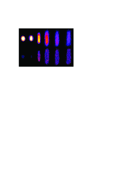
Figure 4: Aspects of the excited cloud during free expansion and the distribution of the fluctuations obtained by subtracting the averaged profile.

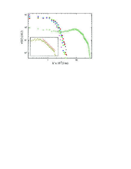
Figure 5: Evolution of the projected momentum distribution measured by time of flight.

In more detail, the studied sequence of nonequilibrium states, observed in experiments [152, 153, 154, 155] and modeled in computer simulations [156, 157, 158, 159, 160, 161, 162] is discussed below.

19.1 Weak nonequilibrium

At the beginning of the process of imposing an alternating potential, when the injected energy $E_{inj}$ is yet insufficient for the creation of coherent modes, being less than twice the energy $E_{emb}$ required for creating at least a couple of embryos, or germs, of vortex rings,

$$0~{}<~{}E_{inj}~{}<~{}2E_{emb}\;,$$ (210)

the trapped atomic cloud is only slightly perturbed with small density fluctuations. Vortex embryos appear by pairs, since each of them possesses vorticity $\pm 1$, while the vorticity of the whole system is zero, which requires that each vortex has to be compensated by an antivortex. The energy of creating a vortex embryo, $E_{emb}$, is smaller then that sufficient for generating a vortex ring, $E_{ring}$. For estimates, it is possible to accept that $E_{emb}\sim E_{ring}/2$.

Let us bring attention of the reader that the injected energy (208) is defined as the energy per particle. Therefore to compare it with the energies of coherent modes, the corresponding energies below are also defined as characteristic reduced energies, that is the energies per particle.

19.2 Vortex embryos

When the injected energy reaches the level sufficient for generating a pair of vortex embryos, these objects arise being just pieces of broken vortex rings. This happens when the injected energy is in the interval

$$2E_{emb}~{}<~{}E_{inj}~{}<~{}2E_{ring}\;.$$ (211)

The embryos can be of different sizes. They have vorticity $\pm 1$. If the external pumping is switched off after the germs are created, they survive for about $0.2$ s, when they do not move, exhibiting only small oscillations. The local equilibration time is

$$t_{loc}~{}=~{}\frac{m}{\hbar\rho a_{s}}~{}=~{}\frac{87.8}{(g\nu)^{2/5}\omega_{x}}\;,$$

which is $t_{loc}\approx 10^{-3}$ s. Since the embryos lifetime of $0.2$ s is much larger than the local equilibration time, the embryos are metastable objects. Typical vortex embryos are shown in Fig. 6 obtained from numerical simulation.

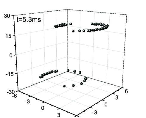
Figure 6: Typical example of vortex germs. The time of the trap modulation is $t=5.3$ ms.

19.3 Vortex rings

The following pumping leads to the appearance of well formed rings of different radii $R_{ring}$, as in Fig. 7 representing numerical results. A vortex ring is a circular line of zero density, with a winding number $\pm 1$ around each of the line elements [163, 164, 165, 166, 167, 168]. The rings with opposite vorticity appear by pairs. These ring modes exist in the interval of energies

$$2E_{ring}~{}<~{}E_{inj}~{}<~{}2E_{vort}\;,$$ (212)

where $E_{vort}$ is the energy of a vortex line. The reduced energy of a ring is

$$E_{ring}~{}=~{}\frac{2\pi^{2}}{N}\;\rho\;R_{ring}\;l_{x}^{2}\;\ln\left(2.25\;\frac{R_{ring}}{l_{coh}}\right)\;\omega_{x}\;.$$ (213)

Here $R_{ring}$ is the ring radius, $l_{coh}$ is the coherence length, and $\rho$ is the density of the system at the location of the ring, if the ring would be absent. In the trap, the ring oscillates [169, 170] with the period

$$T_{ring}~{}=~{}\frac{4\pi R}{l_{coh}\omega_{z}\sqrt{\ln(R/l_{coh})}}~{}=~{}\frac{4\pi(g\nu)^{2/5}}{\omega_{z}\sqrt{\ln(0.5g\nu)}}\;,$$ (214)

which, for the accepted parameters, makes $T_{ring}\approx 0.7$ s. If the pumping is switched off, the ring lifetime is about $0.1$ s, which is much longer than the local equilibration time $t_{loc}\approx 10^{-3}$ s. This shows that the rings are metastable objects. In the trap, the rings look as practically immovable. A pair of rings, found in numerical simulation, is shown in Fig. 7.

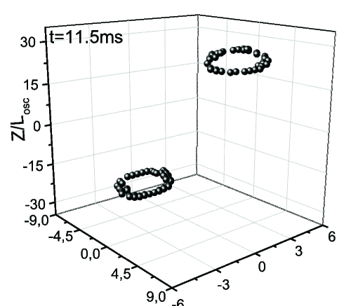
Figure 7: Typical example of vortex rings. The time of the trap modulation is $t=11.5$ ms.

19.4 Vortex lines

The continuing pumping leads to the generation of pairs of vortex lines in the energy interval

$$2E_{vort}~{}<~{}E_{inj}~{}<~{}E_{turb}\;,$$ (215)

in which $E_{turb}$ is the pumped energy after which vortex turbulence develops. Vortices can have different lengths $L_{vort}$. The reduced energy of a vortex of length $L_{vort}$, in the Thomas-Fermi approximation [171], reads as

$$E_{vort}~{}=~{}\frac{2\pi}{3N}\;\rho\;L_{vort}\;l_{x}^{2}\;\ln\left(0.95\;\frac{R}{l_{coh}}\right)\;\omega_{x}\;.$$ (216)

The vortex length $L_{vort}$ is approximately about the cloud length $L$. Then the reduced vortex energy is $E_{vort}=0.296\omega_{x}$.

The vortices move randomly due to the Magnus force caused by the difference in pressure between the opposite sides of a vortex line. The vortex lifetime, after switching off the pumping, is about $0.2$ s. Numerically found vortex lines are shown in Fig. 8.

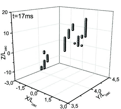
Figure 8: Typical example of vortex lines directed along the $z$ axis. The time of the trap modulation is $t=17$ ms.

19.5 Vortex turbulence

Injecting into the trap more energy creates more and more vortices and anti-vortices, as well as distorts their straight lines and forces them to incline in different directions. The used modulating potential does not impose a rotation axis, because of which the increasing number of vortices does not lead to the creation of a vortex lattice, but results in the formation of a random vortex tangle corresponding to the definition of Vinen quantum turbulence [172, 173, 174, 175, 176, 177]. Being released from the trap, the atomic cloud expands isotropically, which is typical of Vinen turbulence [152, 153, 154, 178].

Vortex turbulence exists in the energy interval

$$E_{turb}~{}<~{}E_{inj}~{}<~{}E_{drop}\;,$$ (217)

where $E_{drop}$ is the upper boundary of the vortex turbulence.

One distinguishes random vortex turbulence, or Vinen turbulence, as opposed to the correlated vortex turbulence, or Kolmogorov turbulence [176]. In a Vinen vortex tangle, the intervortex distance is much larger than the coherence length. Therefore, the summary energy of vortices in the random Vinen tangle can be approximated by the product of the vortex number and a single vortex energy. Thus the vortex turbulence energy threshold

$$E_{turb}~{}=~{}E_{vort}\;N_{vort}$$ (218)

is reached after the injected energy creates the critical number of vortices $N_{vort}$ that is so large that the mean distance between the outer parts of the vortices becomes equal to their diameter $2\xi$, so that no vortex can be inserted inbetween without touching the neighbors. This implies that in the cross-section of the trap the number $N_{vort}$ is such that the equality

$$N_{vort}\pi(4\xi)^{2}~{}=~{}\pi R^{2}$$

holds true. Hence the critical number of vortices is

$$N_{vort}~{}=~{}\left(\frac{R}{4\xi}\right)^{2}\;.$$ (219)

For the experiments with ⁸⁷ Rb, the atomic cloud radius is $R\approx 4\times 10^{-4}$ cm and the coherence length is $\xi\approx 2\times 10^{-5}$ cm. Thus, the critical vortex number is $N_{vort}\approx 25$, which is in perfect agreement with both experiments and numerical simulations.

The overwhelming majority of vortices usually have the lowest circulation number $\pm 1$. In the case where there would arise vortex lines with different circulation, it is possible to represent the system as a mixture of fluids containing vortex lines with different vorticity [179].

The column integrated radial momentum distribution obeys a power law $n_{r}(k)\propto k^{-\gamma}$ in the range $\pi/\xi<k<2\pi/\xi$, which is a key quantitative expectation for an isotropic turbulent cascade [180]. This power low has been observed [181, 182] for turbulent atomic clouds of trapped atoms, with the slope characterized by $\gamma\approx 2$.

It is interesting to note that there exists a similar effect in laser media, which is called optical turbulence or turbulent photon filamentation. In high Fresnel lasers and nonlinear media there appear bright filaments randomly distributed in the sample cross-section and not correlated with each other. The theory of the photon turbulence is developed in Refs. [183, 184, 185]. This effect has been observed in many experiments, as can be inferred from review articles [186, 187, 188, 189, 190, 191, 192, 193, 194].

19.6 Droplet state

Starting from an equilibrium state of a practically completely Bose-condensed system, and injecting energy into the trap by applying an alternating field, we produce more and more excited condensate. In weak nonequilibrium, the whole atomic cloud is yet Bose-condensed. The appearing vortex excitations, such as vortex embryos, vortex rings, and vortex lines can be treated as germs, or nuclei, of uncondensed phase. The following pumping of energy into the trap little by little destroys the condensate. When the injected energy reaches the threshold value $E_{drop}$, vortex turbulence transforms into a new state composed of coherent Bose-condensed droplets immersed into an incoherent surrounding.

The state of coherent droplets is analogous to heterophase states where different thermodynamic phases are intermixed on mesoscopic scale [195, 196, 197]. This state exists in the energy interval

$$E_{drop}~{}<~{}E_{inj}~{}<~{}E_{c}\;,$$ (220)

where $E_{c}$ is the critical amount of energy after which Bose-Einstein condensate is completely destroyed and the lower energy threshold can be estimated as

$$E_{drop}~{}=~{}E_{vort}\;N^{*}_{vort}\;.$$ (221)

Here $N_{vort}^{*}$ is the maximal number of vortices that do not yet essentially interact with each other, so that their centers are separated by the distance $d_{int}$, which defines the number of vortices

$$N_{vort}^{*}~{}=~{}\left(\frac{R}{d_{int}}\right)^{2}\;.$$ (222)

With $R\approx 4\times 10^{-4}$ cm and $d_{int}\approx 0.7\times 10^{-4}$ cm, we have $N_{vort}^{*}\approx 30$, which is in good agreement with experiments. Since $E_{vort}=0.296\omega_{x}$, the energy, after which the droplet state develops is $E_{drop}\approx 8.88\omega_{x}$.

The droplet state develops because the number of vortices becomes so large and their interactions so strong that vortices destroy each other. Numerical simulations show that the grains have the sizes close to the coherence length $\xi\approx 10^{-5}$ cm. The phase inside a grain is constant, hence the grains represent coherent droplets. After switching off the pumping by an alternating potential, each grain survives during the lifetime $10^{-2}$ s, which is much longer than the local equilibration time of $10^{-4}$ s. This tells us that, the droplets are metastable objects. The density inside a droplet is up to $100$ times larger than that of their incoherent surrounding. The number of atoms in a droplet is around $40$. The coherent droplets, whose number is about $400$, are randomly distributed inside the trap.

Figure 9 shows experimentally measured density distributions for different states: vortex state with several vortices (a); vortex turbulence (b); and droplet state (c).

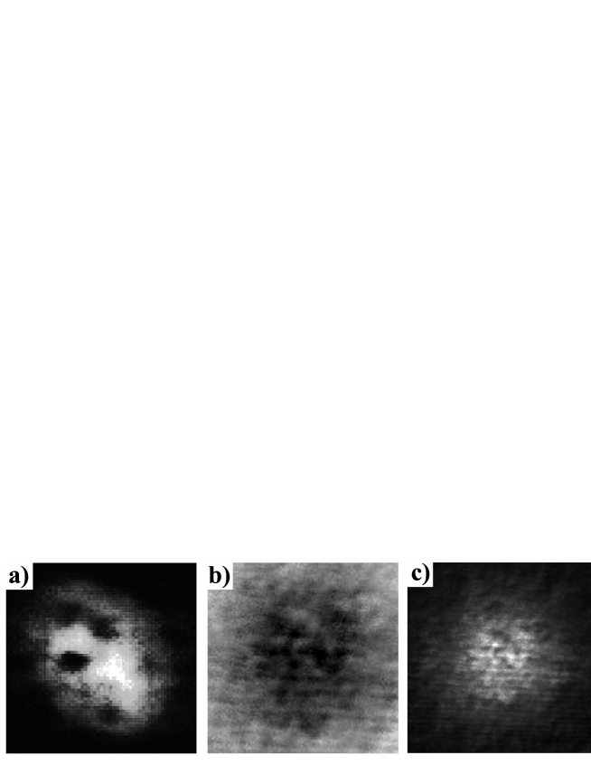
Figure 9: Density distributions for different states, observed in experiments: (a) vortex state with several vortices; (b) vortex turbulence; (c) droplet state.

The droplet state can be called heterophase droplet mixture, droplet turbulence, or grain turbulence. It also reminds fog. In numerical simulations, considering the opposite process of equilibrium Bose-condensate formation from an uncondensed gas, this regime is termed strong turbulence [180, 198]. Since the location of droplets in space is random, after averaging over spatial configurations, the system looks as a mesoscopic mixture of two phases with different density [199, 200]. It is possible to show that the averaging over phase configurations is similar to the averaging over time [201].

19.7 Wave turbulence

After the energy injected into the trap reaches the value $E_{c}=k_{B}T_{c}$, with $T_{c}$ being the Bose-Einstein condensation temperature, the condensed state cannot exist. Then there develops a state modeling the turbulent normal state. This state corresponds to what is termed wave turbulence or weak turbulence. These waves are not so big, with the density only about $3$ times larger than their surrounding. The typical size of a wave is of order $10^{-4}$ cm. The phase inside it is random, which is in line with the absence of Bose-Einstein condensate. However, strictly speaking, the transition between the droplet state and wave turbulence is a gradual crossover. The crossover line, conditionally separating the regimes of droplet state and wave turbulence, can be located at the point, where the system coherence, associated with droplets, is destroyed in half of the system. For ⁸⁷Rb atoms, the critical temperature is $T_{c}=2.76\times 10^{-7}$ K, hence $E_{c}=27.4\omega_{x}$.

20 Classification of states

The described nonequilibrium states can be distinguished by the intervals of injected energy, keeping in mind the relations $E_{emb}\approx 0.5E_{ring}$ and $E_{ring}\approx\nu E_{vort}$, with $\nu=0.11$. Then the characteristic energies are:

$$E_{emb}~{}=~{}0.016\omega_{x}\;,\qquad E_{ring}~{}=~{}0.033\omega_{x}\;,$$

$$E_{vort}~{}=~{}0.296\omega_{x}\;,\qquad E_{turb}~{}=~{}7.4\omega_{x}\;,$$

$$E_{drop}~{}=~{}8.88\omega_{x}\;,\qquad E_{c}~{}=~{}27.4\omega_{x}\;.$$ (223)

Introducing the dimensionless injected energy $E\equiv E_{inj}/\omega_{x}$, it is possible to list the related energy intervals as follows:

$$\begin{array}[]{rlllll}0&<&E&<&0.032{}{}{}&~{}~{}~{}(weak\;nonequilibrium)\;,\\ 0.032&<&E&<&0.066{}{}{}&~{}~{}~{}(vortex\;embryos)\;,\\ 0.066&<&E&<&0.592{}{}{}&~{}~{}~{}(vortex\;rings)\;,\\ 0.592&<&E&<&7.4{}{}{}&~{}~{}~{}(vortex\;lines)\;,\\ 7.4&<&E&<&8.88{}{}{}&~{}~{}~{}(vortex\;turbulence)\;,\\ 8.88&<&E&<&27.4{}{}{}&~{}~{}~{}(coherent\;droplets)\;,\\ &&E&>&27.4{}{}{}&~{}~{}~{}(wave\;turbulence)\;.\end{array}$$ (231)

When a system, prepared in a strongly nonequilibrium symmetric state, equilibrates to a state with broken symmetry, there appear topological defects, such as vortices, protodomains, cells, grains, strings, and monopoles. This is called the Kibble-Zurek mechanism [202, 203, 204, 205]. In our experiments, the opposite procedure of generating nonequilibrium states with topological modes is realized, which can be called inverse Kibble-Zurek scenario [158].

The nonequilibrium states can also be characterized [161, 162] by effective temperature, Fresnel, and Mach numbers. The effective temperature is given by the relation

$$T_{eff}~{}\equiv~{}\frac{2}{3}\;[\;E_{kin}(t)-E_{kin}(0)\;]\;,$$ (232)

where $E_{kin}(t)$ is the current kinetic energy per particle and $E_{kin}(0)$ is the initial kinetic energy of the system at equilibrium. The Fresnel number can be defined as

$$F~{}\equiv~{}\frac{\pi R^{2}}{\lambda L}\qquad\left(\lambda\equiv\sqrt{\frac{2\pi}{mT_{eff}}}\right)\;,$$ (233)

with $\lambda$ being thermal wavelength. And the Mach number is written as

$$M~{}\equiv~{}\frac{v}{c}~{}=~{}\sqrt{\frac{3T_{eff}}{mc^{2}}}\;,$$ (234)

where $v$ is the particle velocity corresponding to the kinetic energy and $c$ is the sound velocity in the system. The classification of the nonequilibrium states of trapped ${}^{87}Rb$ is summarized in Table 1. The values of effective temperature, Fresnel number and Mach number correspond to the lower boundary of the related states, where these states appear.

Table 1: Nonequilibrium states of a trapped Bose-Einstein condensate, characterized by effective temperature (in units of $\omega_{x}$), Fresnel number, and mach number. The figures correspond to the lower boundary of the related states.

Nonequilibrium states	Effective temperature	Fresnel number	Mach number
wave turbulence	23.5	1.01	1.07
coherent droplets	8.56	0.61	0.66
vortex turbulence	5.54	0.49	0.53
vortex lines	2.26	0.31	0.25
vortex rings	1.21	0.23	0.22
vortex embryos	0.29	0.11	0.08
weak nonequilibrium

21 Atom laser

If trapped atoms could be ejected from the trap, this would remind the action of a laser emitting photons. Bose-Einstein condensate is a coherent system, hence emitting Bose-condensed atoms would be similar to emitting coherent light. Thus, one compares with the optical laser the simple process of Bose atoms falling out of the trap under the influence of gravity [206, 207, 208, 209, 210]. The direction of an atomic beam can be regulated by means of Raman scattering [211]. A mechanism allowing for guiding atomic beams in any required direction has been proposed and analyzed in Refs. [212, 213, 214, 215].

Let us consider a system of atoms, with spin operators $S_{i}$, with interaction potential $\Phi_{ij}$, in a magnetic field ${\bf B}_{i}$, and subject to the Earth gravity force ${\bf g}$. The Hamiltonian is

$$H~{}=~{}\sum_{i=1}^{N}\left(-\;\frac{\nabla_{i}^{2}}{2m}\;-\;\mu_{S}\;{\bf S}_{i}\cdot{\bf B}_{i}-m\;{\bf g}\cdot{\bf r}_{i}\right)+\frac{1}{2}\sum_{i\neq j}\Phi_{ij}\;.$$ (235)

Here $\mu_{S}$ is the atomic magnetic moment that can be positive or negative. Since magnetic moments of atoms are often mainly due to electrons, for concreteness, we assume that $\mu_{S}<0$, although the results do not principally depend on the sign of the magnetic moment.

Denoting the quantum-mechanical average by angular brackets, it is straightforward to derive the evolution equations for the mean position vector,

$$m\;\frac{d^{2}}{dt}\;\langle\;{\bf r}_{i}\;\rangle~{}=~{}\mu_{S}\langle\;\vec{\nabla}_{i}({\bf S}_{i}\cdot{\bf B}_{i})\;\rangle-\sum_{j(\neq i)}^{N}\langle\;\vec{\nabla}_{i}\;\Phi_{ij}\;\rangle+m\;{\bf g}\;,$$ (236)

and the average spin,

$$\frac{d}{dt}\;\langle\;{\bf S}_{i}\;\rangle~{}=~{}\mu_{S}\;\langle\;{\bf S}_{i}\times{\bf B}_{i}\;\rangle\;.$$ (237)

Being interested in the motion of an atomic cloud as a whole, we introduce the center-of-mass vector

$${\bf R}~{}\equiv~{}\frac{1}{N}\sum_{i=1}^{N}\langle\;{\bf r}_{i}\;\rangle\;,$$ (238)

the average spin

$${\bf S}~{}\equiv~{}\;\frac{1}{N}\sum_{i=1}^{N}\langle\;{\bf S}_{i}\;\rangle\;,$$ (239)

and the collision force

$${\bf I}~{}\equiv~{}-\;\frac{1}{N}\sum_{i\neq j}^{N}\langle\;\vec{\nabla}_{i}\;\Phi_{ij}\;\rangle$$ (240)

due to atomic interactions.

Assume that the magnetic field is slowly varying in space, so that

$${\bf B}_{i}~{}\equiv{\bf B}({\bf r}_{i})~{}\cong~{}{\bf B}({\bf R})~{}\equiv~{}{\bf B}.$$ (241)

Then the approximate equalities are valid:

$$\frac{1}{N}\sum_{i=1}^{N}\langle\;\vec{\nabla_{i}}({\bf S}_{i}\cdot{\bf B}_{i})\;\rangle~{}\cong~{}\vec{\nabla}({\bf S}\cdot{\bf B})\;,$$

$$\frac{1}{N}\sum_{i=1}^{N}\langle\;{\bf S}_{i}\times{\bf B}_{i}\;\rangle~{}\cong~{}{\bf S}\times{\bf B}\;.$$

Therefore, we have the equations of motion for the center of mass

$$m\;\frac{d^{2}{\bf R}}{dt^{2}}~{}=~{}\mu_{S}\vec{\nabla}({\bf S}\cdot{\bf B})+{\bf I}+m{\bf g}$$ (242)

and for the average spin

$$\frac{d{\bf S}}{dt}~{}=~{}\mu_{S}\;{\bf S}\times{\bf B}\;.$$ (243)

The magnetic field of the trap can be taken in the typical of magnetic traps form [216, 217, 218], as the sum

$${\bf B}~{}=~{}{\bf B}_{1}+{\bf B}_{2}$$ (244)

of a quadrupole field

$${\bf B}_{1}~{}=~{}B_{1}^{\prime}\;(R_{x}{\bf e}_{x}+R_{y}{\bf e}_{y}-\lambda R_{z}{\bf e}_{z})\qquad(B_{1}^{\prime}>0)$$ (245)

and a transverse field

$${\bf B}_{2}~{}=~{}B_{2}(h_{x}{\bf e}_{x}+h_{y}{\bf e}_{e})\qquad(B_{2}>0)\;,$$ (246)

where

$$h_{x}^{2}+h_{y}^{2}~{}=~{}1\qquad(B_{2}=|\;{\bf B}_{2}\;|)\;.$$

There exist two types of quadrupole traps, dynamic quadrupole traps, with the transverse field depending on time,

$$h_{x}~{}=~{}\cos(\omega t)\;,\qquad h_{y}~{}=~{}\sin(\omega t)\;,$$ (247)

and static quadrupole traps, with a time-independent transverse field,

$$h_{x}~{}=~{}const\;,\qquad h_{y}~{}=~{}const\;.$$ (248)

Also, there can exist an additional so-called cooling field serving for removing fast atoms from the center of the trap. However this cooling field does not play role in describing the mechanism of creating directed atomic beams [213].

The method we are suggesting does not depend on whether a dynamic or static trap is accepted [219, 220]. For concreteness, below we illustrate the results for the dynamic quadrupole trap.

The spatial motion of the center of mass is characterized by the frequency $\omega_{1}$ defined by the equation

$$\omega_{1}^{2}~{}=~{}-\;\frac{\mu_{S}(B_{1}^{\prime})^{2}}{mB_{2}}~{}>~{}0\;,$$ (249)

while the spin motion is characterized by the Zeeman frequency

$$\omega_{2}~{}=~{}-\mu_{S}B_{2}~{}>~{}0\;.$$ (250)

We stress that these frequencies are positive, keeping in mind that $\mu_{S}<0$.

The spin motion is faster than the spatial atomic motion, which implies that $\omega_{2}\gg\omega_{1}$. The rotation of the transverse field is faster than the atomic motion, $\omega\gg\omega_{1}$, but slower than the spin motion in order not to induce transitions between the Zeeman energy levels, hence $\omega\ll\omega_{2}$. Thus there are the relations

$$\omega_{1}~{}\ll~{}\omega~{}\ll~{}\omega_{2}\;.$$ (251)

The size of the atomic cloud is defined by the effective radius

$$R_{0}~{}\equiv~{}\frac{B_{2}}{B_{1}^{\prime}}\;.$$ (252)

This radius can be used for defining dimensionless spatial variables describing the location of the center of mass,

$${\bf r}~{}\equiv~{}\frac{{\bf R}}{R_{0}}~{}=~{}\{x,y,z\}\;.$$ (253)

Let us introduce the collision rate $\gamma$ by the equality

$$\gamma\vec{\xi}~{}\equiv~{}\frac{{\bf I}}{mR_{0}}\;.$$ (254)

The cloud of trapped atoms is rarified, so that the collision rate is small, in the sense that

$$\gamma~{}\ll~{}\omega_{1}\;,$$ (255)

and $\xi$ can be approximated by a random variable centered at zero because of the random directions of gradients in the collision force (240).

The shape of the trap can be described by a shape factor, which can be defined by the function

$$f({\bf r})~{}=~{}\exp\left\{-\;\frac{x^{2}+y^{2}}{(R/R_{0})^{2}}\;-\;\frac{z^{2}}{(L/R_{0})^{2}}\right\}\;,$$ (256)

where the trap radius $R\geq R_{0}$ and the trap length $L\geq R_{0}$, or by a step-like function

$$f({\bf r})~{}=~{}1-\Theta\left(x^{2}+y^{2}\;-\;\frac{R^{2}}{R_{0}^{2}}\right)\;\Theta\left(|\;z\;|-\;\frac{L}{2R_{0}}\right)\;.$$ (257)

As we have checked, the concrete choice of the shape factor does not change the overall picture and does not influence the described mechanism [219, 220].

Thus, the center-of-mass spatial motion is given by the equation

$$\frac{d^{2}{\bf r}}{dt^{2}}~{}=~{}\left(\;{\bf F}+\gamma\vec{\xi}\;\right)\;f+\frac{{\bf g}}{R_{0}}\;,$$ (258)

with $f=f({\bf r})$ and the force

$${\bf F}~{}=~{}-\omega_{1}\;(S_{x}{\bf e}_{x}+S_{y}{\bf e}_{y}-\lambda S_{z}{\bf e}_{z})\;.$$ (259)

The spin motion, characterized by equation (243), can be represented as

$$\frac{d{\bf S}}{dt}~{}=~{}\omega_{2}\hat{A}{\bf S}\;,$$ (260)

with an antisymmetric matrix $\hat{A}=[A_{\alpha\beta}]$ having the elements

$$A_{\alpha\alpha}~{}=~{}0\;,\qquad A_{\alpha\beta}~{}=~{}-A_{\beta\alpha}\;,\qquad A_{21}=\lambda\;z\;,$$

$$A_{23}~{}=~{}x+h_{x}\;,\qquad A_{31}~{}=~{}y+h_{y}\;.$$ (261)

According to condition (251), the transverse field (247), rotating with the frequency $\omega$, is fast, as compared to the atomic motion characterized by the frequency $\omega_{1}$. Then, it is possible to resort to the averaging method [221], following which, we find the solution to the fast variable, that is the spin ${\bf S}$, keeping the slow variables, that is the atomic coordinates ${\bf r}$, fixed, and substitute the found fast solution to the equation for the slow variable (258), with averaging the right-hand side of this equation over the random variable $\vec{\xi}$ and over time (see details in Refs. [222, 223, 224]). Thus we come to the equation

$$\frac{d^{2}{\bf r}}{dt^{2}}~{}=~{}{\bf F}_{eff}\;f+\frac{{\bf g}}{R_{0}}\;,$$ (262)

where $f=f({\bf r})$ and the effective force is

$${\bf F}_{eff}~{}=~{}-\;\frac{\omega_{1}^{2}[\;(1+x)S_{0}^{x}+yS_{0}^{y}-\lambda zS_{0}^{z}\;](x{\bf e}_{x}+y{\bf e}_{y}+2\lambda^{2}z{\bf e}_{z})}{2[\;(1+2x+x^{2}+y^{2}+\lambda^{2}z^{2})(1+x^{2}+y^{2}+\lambda^{2}z^{2})\;]^{1/2}}\;.$$ (263)

Here $S_{0}^{\alpha}$ is the initial spin polarization.

The standard initial spin polarization is $S_{0}^{x}=S>0$ and $S_{0}^{y}=S_{0}^{z}=0$. This guarantees atomic confinement for $r<1$, with the attractive effective force

$${\bf F}_{eff}~{}\cong~{}-\;\frac{1}{2}\;\omega_{1}^{2}\;S\;(x{\bf e}_{x}+y{\bf e}_{y}+2\lambda^{2}z{\bf e}_{z})\;,$$

leading to the effective potential well

$$U_{eff}~{}\cong~{}\frac{1}{4}\;\omega_{1}^{2}\;S\;(x^{2}+y^{2}+2\lambda^{2}z^{2})\;.$$

On the contrary, we suggest to arrange the initial spin polarization under conditions

$$S_{0}^{x}~{}=~{}S_{0}^{y}~{}=~{}0\;,\qquad S_{0}^{z}~{}=~{}S\;,$$ (264)

which results in the effective force

$${\bf F}_{eff}~{}=~{}\frac{\omega_{1}^{2}\lambda Sz(x{\bf e}_{x}+y{\bf e}_{y}+2\lambda^{2}z{\bf e}_{z})}{2[\;(1+2x+x^{2}+y^{2}+\lambda^{2}z^{2})(1+x^{2}+y^{2}+\lambda^{2}z^{2})\;]^{1/2}}\;.$$ (265)

If the spin polarization has been aligned with the axis $x$, then the desired initial spin polarization (264) along the axis $z$ can be prepared [225] by the action of an oscillating $\pi/2$ pulse with the frequency in resonance with $\omega_{2}$, turning the spin from the axis $x$ to the axis $z$.

Let us denote a dimensionless gravity acceleration

$$\vec{\delta}~{}\equiv~{}\frac{{\bf g}}{R_{0}\lambda S\omega_{1}^{2}}~{}=~{}\frac{m{\bf g}}{|\;\lambda S\mu_{s}B_{1}^{\prime}\;|}\;.$$ (266)

Then equations (262) acquire the form

$$\frac{d^{2}x}{dt^{2}}~{}=~{}\frac{1}{2}\;z\;x\;f+\delta_{x}\;,$$

$$\frac{d^{2}y}{dt^{2}}~{}=~{}\frac{1}{2}\;z\;y\;f+\delta_{y}\;,\qquad\frac{d^{2}z}{dt^{2}}~{}=~{}\lambda^{2}\;z^{2}\;f+\delta_{z}\;.$$ (267)

The detailed analysis of these equations at small $x$, $y$, and $z$, as well as numerical solution for arbitrary spatial coordinates, demonstrate the effect of atomic semiconfinement [212, 213, 214, 215, 219, 220, 222, 223, 224], when atoms are confined from one side of the trap, but are expelled from another side. In the present setup, atoms are ejected in the direction of the trap axis, with $z>0$. The typical trajectories of the emitted atomic beams are shown in Fig. 10 for the trap axis $z$ inclined by $45$ degrees to the horizon, so that $\delta_{z}=-\delta_{x}$; the initial spatial location of the atomic cloud center of mass is close to the trap center and the initial dimensionless velocities are close to zero, being varied in the interval $-0.1\leq v_{0}^{\alpha}<0.1$. The aspect ratio $\nu=<x>^{2}/<z>^{2}$ is rather small, being $10^{-4}$, which means that the atomic beam is stretched in the $z$ direction about $100$ times larger then in the $x$ direction, that is the beam is very well collimated. The collimation is not essentially influenced by thermal fluctuations, provided the temperature is less than the critical temperature

$$T_{c}~{}\approx~{}\frac{\hbar\omega_{1}^{3}}{k_{B}\gamma^{2}}\;,$$

which is close to the Bose condensation temperature. After leaving the trap, the trajectories become curved due to gravity. The velocity of emitted atoms depends on the setup parameters. For realistic parameters, the velocity can reach $100$ cm/s.

         

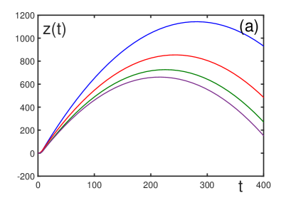
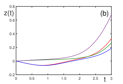
Figure 10: Typical trajectories for the trap parameters $L=40$, $R=1$, $\lambda=10$, the gravity components $\delta_{x}=0.03$, $\delta_{z}=-\delta_{x}$, $\delta_{y}=0$, and different velocities $-0.1<\dot{r}<0.1$: (a) for the time interval $0\leq t\leq 400$; (b) beginning of the process;

22 Conclusion

The problem of generating non-ground-state Bose-Einstein condensates is discussed. Such non-ground-state Bose condensates are represented by nonlinear coherent modes of trapped atoms. Coherent modes are the solutions to the stationary nonlinear Schrödinger equation. The solution to the time-dependent nonlinear Schrödinger equation can be expanded over the coherent modes, which leads to the equations for the amplitudes of the fractional mode populations.

The generation of the coherent modes can be realized by alternating external fields, when either an external trapping potential or atomic interactions are modulated. There exist two ways of generation, resonant generation and nonresonant generation. In the resonant generation, the perturbing alternating field does not need to be strong, but the alternating frequency has to be in resonance with the transition frequency corresponding to the difference between the energy levels of the ground and excited modes. In the nonresonant generation, the perturbing field has to be sufficiently strong, however there is no need to tune the frequencies to resonant conditions.

In the behaviour of coherent modes, there are many similarities with optical phenomena, such as mode locking, interference patterns, Josephson current, Rabi oscillations, Ramsey fringes, and the occurrence of higher-order resonances related to harmonic generation and parametric conversion. Dynamic transition between mode-locked and mode unlocked regimes is similar to a critical phase transition in a statistical system.

Creating coherent modes in a system of coupled traps or in a deep optical lattice allows for the realization of mesoscopic entanglement of atomic clouds and entanglement production. With coherent modes, one can observe atomic squeezing

Employing nonresonant generation it is possible to form strongly nonequilibrium states of Bose condensates with different topological modes including vortex embryos, vortex rings, vortex lines, and condensate droplets. Such nonequilibrium states as vortex turbulence, droplet turbulence, and wave turbulence can be produced. The nonequilibrium states can be classified by means of effective temperature, Fresnel and Mach numbers. The overall procedure of perturbing an initially equilibrium condensate to nonequilibrium states with topological defects, such as vortex embryos, vortex rings, vortex lines, and condensate droplets is called inverse Kibble-Zurek scenario.

The possibility of producing well collimated atomic beams from atom lasers, which can be guided in any desired direction is described.

This research did not receive any specific grant from funding agencies in the public, commercial, or not-for-profit sectors.

References

- [1] Anderson M H, Ensher J R, Matthews M R, Wieman C E and Cornell E A 1995 Science 269 198
- [2] Bradley C C, Sackett C A, Tollett J J and Hulet R G 1995 Phys. Rev. Lett. 75 1687
- [3] Davis K B, Mewes M O, Andrews M R, van Drutten N J, Durfee D S, Kurn D M and Ketterle W 1995 Phys. Rev. Lett. 75 3969
- [4] Parkins A S and Walls D F 1998 Phys. Rep. 303 1
- [5] Dalfovo F, Giorgini S, Pitaevskii L P and Stringari S 1999 Rev. Mod. Phys. 71 463
- [6] Courteille P W, Bagnato V S and Yukalov V I 2001 Laser Phys. 11 659
- [7] Andersen J O 2004 Rev. Mod. Phys. 76 599
- [8] Yukalov V I 2004 Laser Phys. Lett. 1 435
- [9] Bongs K and Sengstock K 2004 Rep. Prog. Phys. 67 907
- [10] Yukalov V I and Girardeau M D 2005 Laser Phys. Lett. 2 375
- [11] Posazhennikova A 2006 Rev. Mod. Phys. 78 1111
- [12] Yukalov V I 2007 Laser Phys. Lett. 4 632
- [13] Proukakis N P and Jackson B 2008 J. Phys. B 41 203002
- [14] Yurovsky V A, Olshanii M, Weiss D S 2008 Adv. At. Mol. Opt. Phys. 55 61
- [15] Yukalov V I 2011 Phys. Part. Nucl. 42 460
- [16] Yukalov V I 2016 Laser Phys. 26 062001
- [17] Morsch O and Oberthaler M 2006 Rev. Mod. Phys. 78 179
- [18] Moseley C, Fialko O and Ziegler K 2008 Ann. Phys. (Berlin) 17 561
- [19] Yukalov V I 2009 Laser Phys. 19 1
- [20] Krutitsky K V 2016 Phys. Rep. 607 1
- [21] Yukalov V I 2018 Laser Phys. 28 053001
- [22] Yukalov V I, Yukalova E P and Bagnato V S 1997 Phys. Rev. A 56 4845
- [23] Yukalov V I 2006 Laser Phys. 16 511
- [24] Bogolubov N N 1949 Lectures on Quantum Statistics (Kiev: Ryadyanska Shkola)
- [25] Bogolubov, N N 1967 Lectures on Quantum Statistics (New York: Gordon and Breach) Vol. 1
- [26] Bogolubov, N N 1970 Lectures on Quantum Statistics (New York: Gordon and Breach) Vol. 2
- [27] Bogolubov N N 2015 Quantum Statistical Mechanics (Singapore: World Scientific)
- [28] Gross E P 1957 Phys. Rev. 106 161
- [29] Gross E P 1958 Ann. Phys. (N.Y.) 4 57
- [30] Gross E P 1960 Ann. Phys. (N.Y. 9 292
- [31] Gross E P 1961 Nuovo Cimento 20 454
- [32] Wu T T 1961 J. Math. Phys. 2 105
- [33] Pitaevskii L P 1961 J. Exp. Theor. Phys. 13 451
- [34] Gross E P 1963 J. Math. Phys. 4 195
- [35] Malomed B 2005 Nonlinear Schrödinger equations, in Encyclopedia of Nonlinear Science ed Scott A (New York: Routledge) p. 639
- [36] Vinogradov I M 1988 ed Encyclopedia of Mathematics (Dordrecht: Kluwer) Vol. 2 p. 67
- [37] Calogero F and Degasperis A 1982 Spectral Transform and Solitons (Amsterdam: North-Holland)
- [38] Faddeev L D and Takhtajan L A 1987 Hamiltonian Methods in the Theory of Solitons (Berlin: Springer)
- [39] Yukalov V I, Yukalova E P and Bagnato V S 2000 Laser Phys. 10 26
- [40] Bagnato V S, Yukalova E P and Yukalov V I 2000 in Bose-Einstein Condensates and Atom Lasers ed Martelucci S, Chester A, Aspect A and Inguscio M (New York: Kluwer) p. 201
- [41] Yukalov V I, Yukalova E P and Bagnato V S 2001 Laser Phys. 11 455
- [42] Yukalov V I, Yukalova E P and Bagnato V S 2002 Phys. Rev. A 66 043602
- [43] Klauder J R and Skagerstam B S 1985 Coherent States (Singapore: World Scientific)
- [44] Serov V V, Derbov V L, Vinitsky S I and Yukalov V I 2002 Proc SPIE 4706 124
- [45] Yukalov V I, Yukalova E P and Bagnato V S 2002 Laser Phys. 12 1325
- [46] Yukalov V I, Yukalova E P and Bagnato V S 2002 Phys. Rev. A 66 025602
- [47] Allen L and Eberly J H 1975 Optical Resonance and Two-Level Atoms New York: Wiley 1975.
- [48] Yukalov V I, Yukalova E P and Bagnato V S 2003 Laser Phys. 13, 551
- [49] Yukalov V I, Yukalova E P and Bagnato V S 2003 Laser Phys. 13, 861
- [50] Mandel L and Wolf E 1995 Optical Coherence and Quantum Optics (Cambridge: Cambridge University Press)
- [51] Bogolubov N N and Mitropolsky Y A 1961 Asymptotic Methods in the Theory of Nonlinear Oscillations (New York: Gordon and Breach)
- [52] Murdock J A 1991 Perturbations (New York: Wiley)
- [53] Yukalov V I and Yukalova E P 2002 J. Phys. A 35 8603
- [54] Marzlin, K P and Zhang W 1998 Phys. Rev. A 57 3801
- [55] Marzlin, K P and Zhang W 1998 Phys. Rev. A 57 4761
- [56] Ostrovskaya E A, Kivshar, Y S, Lisak M, Hall B, Cattani F and Anderson, D 2000 Phys. Rev. A 61 031601
- [57] Feder D L, Pindzola M S, Collins L A, Schneider B I and Clark C W 2000 Phys. Rev. A 62 053606
- [58] Kivshar Y S, Alexander T J and Turitsyn S K Phys. Lett. A 278 225
- [59] Damski B, Karkuszewski Z P, Sacha K, Zakrewski J 2001 Phys. Rev. A 65 013604
- [60] D’Agosta R, Malomed B A and Precilla C 2002 Laser Phys. 12 37
- [61] Williams J, Walser R, Cooper J, Cornell E A and Holland M 2000 Phys. Rev. A 61 033612
- [62] Nepomnyashchy Y A 1974 Theor. Math. Phys. 20 904
- [63] Yukalov V I 1980 Acta Phys. Pol. A 57 295
- [64] Yukalov V I and Yukalova E P 2004 Laser Phys. Lett. 1 50
- [65] Abad M, Recati A, Stringari S and Frédéric C 2015 Eur. Phys. J. D 69 126
- [66] Yukalov V I 2022 Laser Phys. Lett. 19 103001
- [67] Chandrasekhar S 1961 Hydrodynamics and Hydromagnetic Stability (Oxford: Clarendon Press)
- [68] Kul H J 1991 Phys. Rep. 206 197
- [69] Sasaki K, Suzuki N, Akamatsu D and Saito H 2009 Phys. Rev. A 80 063611
- [70] Takeuchi H, Suzuki N, Kasamatsu K, Saito H and Tsubota M 2010 Phys. Rev. B 81 094517
- [71] Ishino S, Tsubota M and Takeuchi H 2011 Phys. Rev.A 83 063602
- [72] Fujimoto K and Tsubota M 2012 Phys. Rev. A 85 033642
- [73] Yukalov V I 2019 Phys. Part. Nucl. 50 141
- [74] Yukalov V I and Yukalova E P 2021 Physics 3 829
- [75] Yukalov V I, Yukalova E P and Bagnato V S 2001 Proc. SPIE 4243 150
- [76] Yukalov V I, Yukalova E P and Bagnato V S 2002 Laser Phys. 12 231
- [77] Ramos E R, Sanz L, Yukalov V I and Bagnato V S 2007 Phys. Rev. A 76 033608
- [78] Barrett M D, Sauer J A and Chapman M S 2001 Phys. Rev. Lett. 87 010404
- [79] Ryu C, Andersen M F, Clade P, Natarajan V, Helmerson K and Phillips W D 2007 Phys. Rev. Lett. 99 260401
- [80] Yukalov V I, Marzlin K P and Yukalova E P 2004 Phys. Rev. A 69 023620
- [81] Simon B 1970 Helv. Phys. Acta 43 607
- [82] Yukalov V I, Marzlin K P and Yukalova E P 2004 Laser Phys. 14 565
- [83] Yukalov V I, Marzlin K P, Yukalova E P and Bagnato V S 2005 AIP Conf. Proc. 770 218
- [84] Jauregui R, Poli N, Roati G and Modugno G 2001 Phys. Rev. A 64 033403
- [85] Kumakura M, Shirahata Y, Takasu Y, Takahashi Y and Yabuzaki T 2003 Phys. Rev. A 68 021401
- [86] Poli N, Brecha R J, Roati G and Modugno G 2002 Phys. Rev. A 65 021401
- [87] Marzlin K P and Yukalov V I 2005 Eur. Phys. J. D 33 253
- [88] Alberti A, Ferrari G, Ivanov V V, Chiofalo M L and Tino G M 2010 New J. Phys. 12 065037
- [89] Parker C V, Ha L C and Chin C 2013 Nature Phys. 9 769
- [90] Zheng W and Zhai H 2014 Phys. Rev. A 89 061603
- [91] Zhang S L and Zhou Q 2014 Phys. Rev. A 90 051601
- [92] Niu L, Hu D, Jin S, Dong X, Chen X and Zhou X 2015 Opt. Express 23 10064
- [93] Hudomal A, Regnault N and Vasic I 2019 Phys. Rev. A 100 053624
- [94] Boulier T, Maslek J, Bukov M, Bracamontes C, Magnan E, Lellouch S, Demler E, Goldman N and Porto J 2019 Phys. Rev. X 2019 9 011047
- [95] Zheng N, Liu W, Wu J, Li Y, Sovkov V and Ma J 2022 Photonics 9 442
- [96] Cronin A D, Schmiedmayer J and Pritchard, D E 2009 Rev. Mod. Phys. 81 1051
- [97] Milburn G J, Corney J, Wright E M and Walls D F 1997 Phys. Rev. A 55 4318
- [98] Raghavan S, Smerzi A, Fantoni S and Shenoy S R, 1999 Phys. Rev. A 59 620
- [99] Leggett A J 1975 Rev. Mod. Phys. 47 331
- [100] Ohberg P and Stenholm S 1999 Phys. Rev. A 59 3890
- [101] Davis M J and Heller E J 1981 J. Chem. Phys. 75 246
- [102] Heller E J and Davis M J 1981 J. Phys. Chem. 85 307
- [103] Rabi I 1937 Phys. Rep. 51 652
- [104] Yukalov V I 1998 Phys. At. Nucl. 61 1882
- [105] Yukalov V I and Yukalova E P 2000 Phys. Part. Nucl. 31 561
- [106] Ramsey N F 1990 Rev. Mod. Phys. 62 541
- [107] Ramos E R F, Sanz L, Yukalov V I and Bagnato V S 2007 Phys. Lett. A 365 126
- [108] Ramos E R F, Sanz L, Yukalov V I and Bagnato V S 2007 Nucl. Phys. A 790 776
- [109] Eschmann A, Ballagh R J and Caradoc-Davies B M 1999 J. Opt. B: Quantum Semiclass. Opt. 1 383
- [110] Döring D, Debs J E, Robins N P, Figl C, Altin P A and Close J D 2009 Opt. Express 17 20661
- [111] Kokkelmans S J and Holland M J 2002 Phys. Rev. Lett. 89 180401
- [112] Timmermans E, Tommasini P, Hussein M and Kerman A 1999 Phys. Rep. 315 199
- [113] Yukalov V I and Yukalova E P 2005 J. Low Temp. Phys. 138 657
- [114] Ramos E R, Henn E A, Seman J A, Caracanhas M A, Magalhães K M, Helmerson K, Yukalov V I and Bagnato V S 2008 Phys. Rev. A 78 063412
- [115] Yukalov V I and Bagnato V S 2009 Laser Phys. Lett. 6 399
- [116] Nguyen J H V, Tsatsos M C, Luo D, Lode A U J, Telles G D, Bagnato V S and Hulet R G, 2019 Phys. Rev. X 9 011052
- [117] Shukuno N, Sano Y and Tsubota M 2023 J. Phys. Soc. Jap. 92 064602
- [118] Yukalov V I 2005 Phys. Rev. E 72 066119
- [119] Yualov V I 2006 Laser Phys. Lett. 3 406
- [120] Yukalov V I 2006 Phys. Lett. A 359 712
- [121] Yukalov V I 2008 Ann. Phys. (N.Y.) 323 461
- [122] Yukalov V I, Yukalova E P and Sornette D 2013 Laser Phys. Lett. 10 115502
- [123] Yukalov V I, Yukalova E P and Sornette D 2014 J. Phys. Conf. Ser. 497 012034
- [124] Poulsen U V and Mølmer K 2001 Phys. Rev. A 64 013616
- [125] Sørensen A, Duan L M, Cirac J I and Zoller P 2001 Nature 409 63
- [126] Orzel C, Tuchman A K, Fenselau M L, Yasuda M and Kasevich M A 2001 Science 291 2387
- [127] Wineland D J, Bollinger J J, Itano W M and Heinsen D J 1994 Phys. Rev. A 50 67
- [128] Bouyer P and Kasevich M A 1997 Phys. Rev. A 56 1083
- [129] Hadzibabic Z, Stock S, Battelier B, Bretin V and Dalibard J 2004 Phys. Rev. Lett. 93 180403
- [130] Cennini G, Geckeler C, Ritt G and Weitz M 2005 Phys. Rev. A 72 051601
- [131] Yukalov V I 2013 Laser Phys. 23 062001
- [132] Yukalov V I and Yukalova E P 2006 Laser Phys. 16 354
- [133] Keyl M 2002 Phys. Rep. 369 431
- [134] Yukalov V I 2003 Phys. Rev. Lett. 90 167905
- [135] Yukalov V I 2003 Phys. Rev. A 68 022109
- [136] Yukalov V I 2003 Mod. Phys. Lett. B 17 95
- [137] Marcus M and Moyls B N 1959 Pacif. J. Math. 9 1215
- [138] Westwick R 1967 Pacif. J. Math. 23 613
- [139] Beasley L 1988 Linear Algebra Appl. 107 161
- [140] Alfsen E and Shultz F 2010 J. Math. Phys. 51 052201
- [141] Johnston N 2011 Linear Multilinear Algebra 59 1171
- [142] Friedland S, Li C K, Poon Y T and Sze N S 2011 J. Math. Phys. 52 042203
- [143] Gohberg J and Goldberg S 1987 J. Math. Anal. Appl. 125 124
- [144] Fan H Y 2001 Mod. Phys. Lett. B 15 1475
- [145] Yukalov V I and Yukalova E P 2006 Phys. Rev. A 73 022335
- [146] Yukalov V I and Yukalova E P 2008 J. Phys. Conf. Ser. 104 012003
- [147] Yukalov V I and Sornette D 2010 Phys. At. Nucl. 73 559
- [148] Yukalov V I, Yukalova E P and Yurovsky V A 2019 Laser Phys. 29 065502
- [149] Yukalov V I 2020 Entropy 22 565
- [150] Henn E A L, Seman J A, Ramos E R F, Caracanhas M, Castilho P, Olimpio E P, Roati G, Magalhães D V, Magalhães K M F and Bagnato V S 2009 Phys. Rev. A 79 043618
- [151] Seman J A, Henn E A L, Haque M, Shiozaki R F, Ramos E R F, Caracanhas M, Castilho P, Castelo Branco C, Tavares P E S, Poveda-Cuevas F J, Roati G, Magalhães K M F and Bagnato V S 2010 Phys. Rev. A 82 033616
- [152] Henn E A L, Seman J A, Roati G, Magalhães K M F and Bagnato V S 2009 Phys. Rev. Lett. 103 045301
- [153] Shiozaki R F, Telles G D, Yukalov V I and Bagnato V S 2011 Laser Phys. Lett. 8 393
- [154] Seman J A, Henn E A L, Shiozaki R F, Roati G, Poveda-Cuevas F J, Magalhães K M F, Yukalov V I, Tsubota M, Kobayashi M, Kasamatsu K and Bagnato V S 2011 Laser Phys. Lett. 8 691
- [155] Bagnato V S and Yukalov V I 2013 Prog. Opt. Sci. Photon. 1 377
- [156] Yukalov V I, Novikov A N and Bagnato V S 2014 Laser Phys. Lett. 11 095501
- [157] Yukalov V I, Novikov A N and Bagnato V S 2015 J. Low Temp. Phys. 180 53
- [158] Yukalov V I, Novikov A N and Bagnato V S 2015 Phys. Lett. A 379 1366
- [159] Novikov A N, Yukalov V I and Bagnato V S 2015 J Phys. Conf. Ser. 594 012040
- [160] Yukalov V I, Novikov A N, Yukalova E P and Bagnato V S 2016 J. Phys. Conf. Ser. 691 012019
- [161] Yukalov V I , Novikov A N and Bagnato V S 2018 Laser Phys. Lett. 15 065501
- [162] Yukalov V I, Novikov A N, Yukalova E P and Bagnato V S 2020 J. Phys. Conf. Ser. 1508 012006
- [163] Iordanskii S V 1965 J. Exp. Theor. Phys. 21 467
- [164] Amit D and Gross E P 1966 Phys. Rev. 145 130
- [165] Roberts P H and Grant J 1971 J. Phys. A 4 55
- [166] Jones C A and Roberts P H 1982 J. Phys. A 15 2599
- [167] Barenghi C F and Donnelly R J 2009 Fluid Dyn. Res. 41 051401
- [168] Belyaev S T 2016 J. Exp. Theor. Phys. 149 1107
- [169] Jackson B, McCann J F, and Adams C S 1999 Phys. Rev. A 61 013604
- [170] Reichl M D and Mueller E J 2013 Phys. Rev. A 88 053626
- [171] Pethick C J and Smith H 2008 Bose-Einstein Condensation in Dilute Gases (Cambridge: Cambridge University)
- [172] Vinen W F and Niemela J J 2002 J. Low Temp. Phys. 128 167
- [173] Vinen W F 2006 J. Low Temp. Phys. 145 7
- [174] Vinen W F 2010 J. Low Temp. Phys. 161 419
- [175] Tsubota M, Kobayashi M and Takeushi H 2013 Phys. Rep. 522 191
- [176] Nemirovskii S K 2013 Phys. Rep. 524 85
- [177] Tsatsos M C, Tavares P E S, Cidrim A, Fritsch A R, Caracanhas M A, Dos Santos F E A, Barenghi C F and Bagnato V S 2016 Phys. Rep. 622 1
- [178] Caracanhas M, Fetter A, Baym G, Muniz S and Bagnato V S 2013 J. Low Temp. Phys. 170 133
- [179] Yukalov V I 2010 Laser Phys. Lett. 7 467
- [180] Zakharov V E, Lvov V S and Falkovich G 1992 Kolmogorov Spectra of Turbulence (Berlin: Springer)
- [181] Thompson K J, Bagnato G G, Telles G D, Caracanhas M A, Dos Santos F E A and Bagnato V S 2014 Laser Phys. Lett. 11 015501
- [182] Navon N, Gaunt A L, Smith R P and Hadzibabic Z 2016 Nature 532 72
- [183] Yukalov V I 2000 Phys. Lett. A 278 30
- [184] Yukalov V I 2001 Physica A 291 255
- [185] Yukalov V I 2001 Opt. Spectrosc. 91 515
- [186] Akhmanov S A, Sukhorukov A P and Khokhlov R V 1967 Phys. Usp. 93 19
- [187] Lugiato L A 1992 Phys. Rep. 219 293
- [188] Arecchi F T 1995 Physica D 86 297
- [189] Huyet G and Tredicce J R 1996 Physica D 96 209
- [190] Huyet G and Rica S 1996 Physica D 96 215
- [191] Arecchi F T, Boccaletti S and Ramazza P L 1999 Phys. Rep. 318 1
- [192] Calderon O G, Leyva I and Guerra J M 1999 IEEE J. Quantum Electron. 35 1
- [193] Yukalov V I and Yukalova E P 2000 Phys. Part. Nucl. 31 561
- [194] Yukalov V I 2014 Laser Phys. 24 094015
- [195] Yukalov V I 1991 Phys. Rep. 208 395
- [196] Yukalov V I 2003 Int. J. Mod. Phys. B 17 2333
- [197] Yukalov V I and Yukalova E P 2023 Phys. Part. Nucl. 54 1
- [198] Zakharov V E and Nazarenko S V 2005 Physica D 201 203
- [199] Yukalov V I and Yukalova E P 2015 Rom. Rep. Phys. 67 159
- [200] Yukalov V I and Yukalova E P 2015 Laser Phys. 25 035501
- [201] Yukalov V I , Yukalova E P and Bagnato V S 2009 Laser Phys. 19 686
- [202] Kibble T W B 1976 J. Phys. A 9 1387
- [203] Kibble T W B 1980 Phys. Rep. 67 183
- [204] Zurek W H 1985 Nature 317 505
- [205] Zurek W H 1996 Phys. Rep. 276 177
- [206] Mewes M O, Andrews M R, Kurn D M, Durfee D S, Townsend C G and Ketterle W 1997 Phys. Rev. Lett. 78 582
- [207] Bloch I, Hänsch T and Esslinger T 1999 Phys. Rev. Lett. 82 3008
- [208] Bolpasi V, Efremidis N K, Morrissey M J, Condylis P C, Sahagun D, Baker M and von Klitzing W 2014 New J. Phys. 16 033036
- [209] Bennetts S, Chen C C, Pasquiou B and Schreck F 2017 Phys. Rev. Lett. 119 223202
- [210] Chen C C, Escudero R G, Minář J, Pasquiou B, Bennetts S and Schreck F 2022 Nature 606 683
- [211] Hagley E W, Deng L, Kozuma M, Wen J, Helmerson K, Rolston S L and Phillips W D 1999 Science 283 1706
- [212] Yukalov V I 1997 Phys. Rev. A 56 5004
- [213] Yukalov V I 1997 Laser Phys. 7 998
- [214] Yukalov V I 1997 Braz. J. Phys. 27, 260
- [215] Yukalov V I 1999 Phys. Rev. A 60 721
- [216] Petrich W, Anderson M H, Ensher J R and Cornell E A 1995 Phys. Rev. Lett. 74 3352
- [217] Anderson M H, Ensher J R, Matthews M R, Wieman C E and Cornell E A 1995 Science 269 198
- [218] Jin D S, Ensher J R, Matthews M R, Wieman C R and Cornell E A 1996 Phys. Rev. Lett. 77 420
- [219] Yukalov V I and Yukalova E P 1998 Laser Phys. 8 890
- [220] Yukalov V I and Yukalova E P 1999 Laser Phys. 9 531
- [221] Bogolubov N and Mitropolsky Y A 1961 Asymptotic Methods in the Theory of Non-Linear Oscillations (New York: Gordon Breach)
- [222] Yukalov V I and Yukalova E P 1999 Phys. Lett. A 253 173
- [223] Yukalov V I and Yukalova E P 2000 Laser Phys. 10 64
- [224] Yukalov V I and Yukalova E P 2002 Phys. Lett. A 297 412
- [225] Slichter C P 1990 Principles of Magnetic Resonance (Berlin: Springer)