Score Normalization for a
Faster Diffusion Exponential Integrator Sampler

Abstract

Recently, Zhang and Chen [25] have proposed the Diffusion Exponential Integrator Sampler (DEIS) for fast generation of samples from Diffusion Models. It leverages the semi-linear nature of the probability flow ordinary differential equation (ODE) in order to greatly reduce integration error and improve generation quality at low numbers of function evaluations (NFEs). Key to this approach is the score function reparameterisation, which reduces the integration error incurred from using a fixed score function estimate over each integration step. The original authors use the default parameterisation used by models trained for noise prediction – multiply the score by the standard deviation of the conditional forward noising distribution. We find that although the mean absolute value of this score parameterisation is close to constant for a large portion of the reverse sampling process, it changes rapidly at the end of sampling. As a simple fix, we propose to instead reparameterise the score (at inference) by dividing it by the average absolute value of previous score estimates at that time step collected from offline high NFE generations. We find that our score normalisation (DEIS-SN) consistently improves FID compared to vanilla DEIS, showing an improvement at 10 NFEs from 6.44 to 5.57 on CIFAR-10 and from 5.9 to 4.95 on LSUN-Church ($64\times 64$). Our code is available at https://github.com/mtkresearch/Diffusion-DEIS-SN.

1 Introduction

Diffusion models [4, 20] have emerged as a powerful class of deep generative models, due to their ability to generate diverse, high-quality samples, rivaling the performance of GANs [8] and autoregressive models [19]. They have shown promising results across a wide variety of domains and applications including (but not limited to) image generation [2, 17], audio synthesis [12], molecular graph generation [6], and 3D shape generation [16]. They work by gradually adding Gaussian noise to data through a forward diffusion process parameterized by a Markov chain, and then reversing this process via a learned reverse diffusion model to produce high-quality samples.

The sampling process in diffusion models can be computationally expensive, as it typically requires hundreds to thousands of neural network function evaluations to generate high-quality results. Moreover, these network evaluations are necessarily sequential, seriously hampering generation latency. This has motivated recent research efforts to develop acceleration approaches that allow the generation of samples with fewer function evaluations while maintaining high sample quality. Denoising Diffusion Implicit Models (DDIM) [21] is an early but effective acceleration approach that proposes a non-Markovian noising process for more efficient sampling. Song et al. [22] show that samples can be quickly generated by using black-box solvers to integrate a probability flow ordinary differential equation (ODE). Differentiable Diffusion Sampler Search (DDSS) [24] treats the design of fast samplers for diffusion models as a differentiable optimization problem. Diffusion model sampling with neural operator (DSNO) [27] accelerates the sampling process of diffusion models by using neural operators to solve probability flow differential equations. Progressive Distillation [18] introduces a method to accelerate the sampling process by iteratively distilling the knowledge of the original diffusion model into a series of models that learn to cover progressively larger and larger time step sizes.

Recently, a new family of fast samplers, that leverage the semi-linear nature of the probability flow ODE, have enabled new state-of-the-art results at low numbers of function evaluations (NFEs) [13, 26, 25]. In this work we focus on improving the Diffusion Exponential Integrator Sampler (DEIS) [25], specifically the time-based Adams-Bashforth version (DEIS-$t$AB). Our contributions are as follows:

1. We show that DEIS’s default score parameterisation’s average absolute value varies rapidly near the end of the reverse process, potentially leading to additional integration error.

2. We propose a simple new score parameterisation – to normalise the score estimate using its average empirical absolute value at each timestep (computed from high NFE offline generations). This leads to consistent improvements in FID compared to vanilla DEIS.

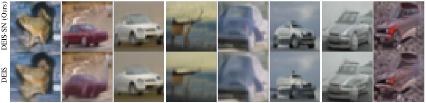
Figure 1: Generations at 5 NFEs with a CIFAR-10 model. Top: DEIS-SN (ours). Bottom: DEIS [25]. It can be seen that DEIS-SN is often able to better generate details (such as wheels on cars). More generation results are shown in Fig. 4 of Appendix D.

2 Preliminaries

Forward Process

We define a forward process over time $t\in[0,1]$ for random variable $\boldsymbol{x}_{t}\in\mathbb{R}^{D}$,

$$p(\boldsymbol{x}_{t}|\boldsymbol{x}_{0})=\mathcal{N}(\boldsymbol{x}_{t};\ a_{t}\boldsymbol{x}_{0},\;\sigma_{t}^{2}\boldsymbol{I})$$ (1)

for $\boldsymbol{x}_{0}$ drawn from some unknown distribution $p(\boldsymbol{x}_{0})$. Here, $a_{t}$ and $\sigma_{t}$ define the noise schedule. The following stochastic differential equation has the same conditional distributions as Eq. 1 [9],

$$d\boldsymbol{x}_{t}=f_{t}\boldsymbol{x}_{t}dt+g_{t}d\boldsymbol{w}_{t},\quad\boldsymbol{x}_{0}\sim p(\boldsymbol{x}_{0}),$$ (2)

where $\boldsymbol{w}_{t}\in\mathbb{R}^{D}$ is the Wiener process and

$$f_{t}=\frac{da_{t}}{dt}\frac{1}{a_{t}},\quad g_{t}^{2}=\frac{d\sigma_{t}^{2}}{dt}-2f_{t}\sigma_{t}^{2}.$$ (3)

Probability Flow ODE

Song et al. [22] show that the following ODE,

$$\frac{d\boldsymbol{x}_{t}}{dt}=f_{t}\boldsymbol{x}_{t}-\frac{1}{2}g^{2}_{t}\nabla_{\boldsymbol{x}_{t}}\log\;p(\boldsymbol{x}_{t}),\quad\boldsymbol{x}_{1}\sim p(\boldsymbol{x}_{1}),$$ (4)

shares the same marginal distributions $p(\boldsymbol{x}_{t})$ as the stochastic differential equation in Eq. 2. Given a neural network that is trained to approximate the score $\boldsymbol{s}_{\theta}(\boldsymbol{x}_{t},t)\approx\nabla_{\boldsymbol{x}_{t}}\log\;p(\boldsymbol{x}_{t})$, Eq. 4 can be exploited to generate samples approximately from $p(\boldsymbol{x}_{0})$ using blackbox ODE solvers [22]. This approach tends to produce higher quality samples at lower NFEs vs stochastic samplers [22]. We note that in the domain of diffusion models, neural networks tend to be trained to predict a parameterisation of the score, e.g. $\boldsymbol{s}_{\theta}(\boldsymbol{x}_{t},t)=-\boldsymbol{\epsilon}_{\theta}(\boldsymbol{x}_{t},t)/\sigma_{t}$ (noise prediction) [4] or $s_{\theta}(\boldsymbol{x}_{t},t)=(a_{t}\boldsymbol{x}_{\theta}(\boldsymbol{x}_{t},t)-\boldsymbol{x}_{t})/\sigma_{t}^{2}$ (sample prediction) [18], as this leads to better optimisation and generation quality [4].

Exponential Integrator

Recently, a number of different approaches have exploited the semi-linear structure of Eq. 4, solving the linear part, $f_{t}\boldsymbol{x}_{t}$, exactly [13, 25, 26, 14]. This has lead to impressive generation quality at low NFEs ($\leq 20$). One such approach is the Diffusion Exponential Integrator Sampler (DEIS) [25] that uses the following iteration over time grid $\{t_{i}\}_{i=0}^{N}$ to generate samples:

$$\boldsymbol{x}_{t_{i-1}} =\Psi(t_{i-1},t_{i})\boldsymbol{x}_{t_{i}}\;+\;\sum_{j=0}^{r}C_{ij}\underbrace{(-K_{t_{i+j}})\boldsymbol{s}_{\theta}(\boldsymbol{x}_{t_{i+j}},t_{i+j})}_{\text{score reparameterisation}},$$ (5)

$$C_{ij} =\int_{t_{i}}^{t_{i-1}}\frac{1}{2}\Psi(t_{i-1},\tau)g_{\tau}^{2}K_{\tau}^{-1}\prod_{k\neq j}\left[\frac{\tau-t_{i+k}}{t_{i+j}-t_{i+k}}\right]d\tau,$$

where $\Psi(t,s)$ satisfies $\frac{\partial\Psi(t,s)}{\partial t}=f_{t}\Psi(t,s),\Psi(s,s)=1$, $K_{t}$ is a function used to reparameterise the score estimate and $r$ is the order of the polynomial used to extrapolate said score reparameterisation. We note that $C_{ij}$ and $\Psi(t,s)$ can be straightforwardly calculated offline using numerical methods.

3 The Importance of Score Reparameterisation

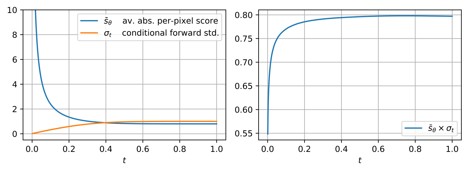
Figure 2: Left: average absolute per-pixel score estimate value $\bar{s}_{\theta}$ and the conditional forward standard deviation $\sigma_{t}$ plotted over the reverse process. Right: the product of the previous two values – we see that this is constant for most of the reverse process, but it changes rapidly near $t=0$. The noising schedule is the Linear $\beta$ schedule [4], the training data is CIFAR-10 and we average 256 samples.

The key to reducing integration error in Eq. 5 is the score reparameterisation. DEIS approximates an integral over $\tau\in[t_{i-1},t_{i}]$, over which $-K_{\tau}\boldsymbol{s}_{\theta}(\boldsymbol{x}_{\tau},\tau)$ should vary, using fixed estimates from finite $t$s. This approximation will be more accurate the less $-K_{\tau}\boldsymbol{s}_{\theta}(\boldsymbol{x}_{\tau},\tau)$ varies with $\tau$. Zhang and Chen [25] choose the default parameterisation for noise prediction models, $K_{t}=\sigma_{t}$, where $\boldsymbol{\epsilon}_{\theta}(\boldsymbol{x}_{t},t)=-\sigma_{t}\boldsymbol{s}_{\theta}(\boldsymbol{x}_{t},t)$. Fig. 2 shows that this reparameterisation (right) is roughly constant in average absolute pixel value ($\bar{s}_{\theta}\sigma_{t}$) for the majority of the generation process, whilst the score estimate varies considerably more. By reducing the variation over time of the score estimate via reparameterisation, DEIS is able to achieve much lower integration error and better quality generations at low NFEs [25].

4 Score Normalisation (DEIS-SN)

Fig. 2 also shows, however, that near $t=0$ there is still substantial variation in $\bar{s}_{\theta}\sigma_{t}$. Thus we propose a new score reparameterisation, where we simply set $K_{t}=1/\bar{s}_{\theta}(t)$. That is to say, at inference, we normalise the score estimate with the empirical average absolute pixel value at $t$ of previous score estimates. The aim of this is to further reduce the variation in the reparameterisation near $t=0$.

$\bar{s}_{\theta}(t)$ can be found using offline generations at high NFEs. We use linear interpolation to accommodate continuous $t$. Our approach can be directly plugged into DEIS, so we refer to it as DEIS-SN.

We note that gDDIM [26] is another extension to DEIS, however this approach is specifically applicable to data distributions that are well modelled by a single Gaussian (such as the velocity of Critically-Damped Langevin Diffusion [3]), which is not the case for image datasets like CIFAR.

5 Experimental Results

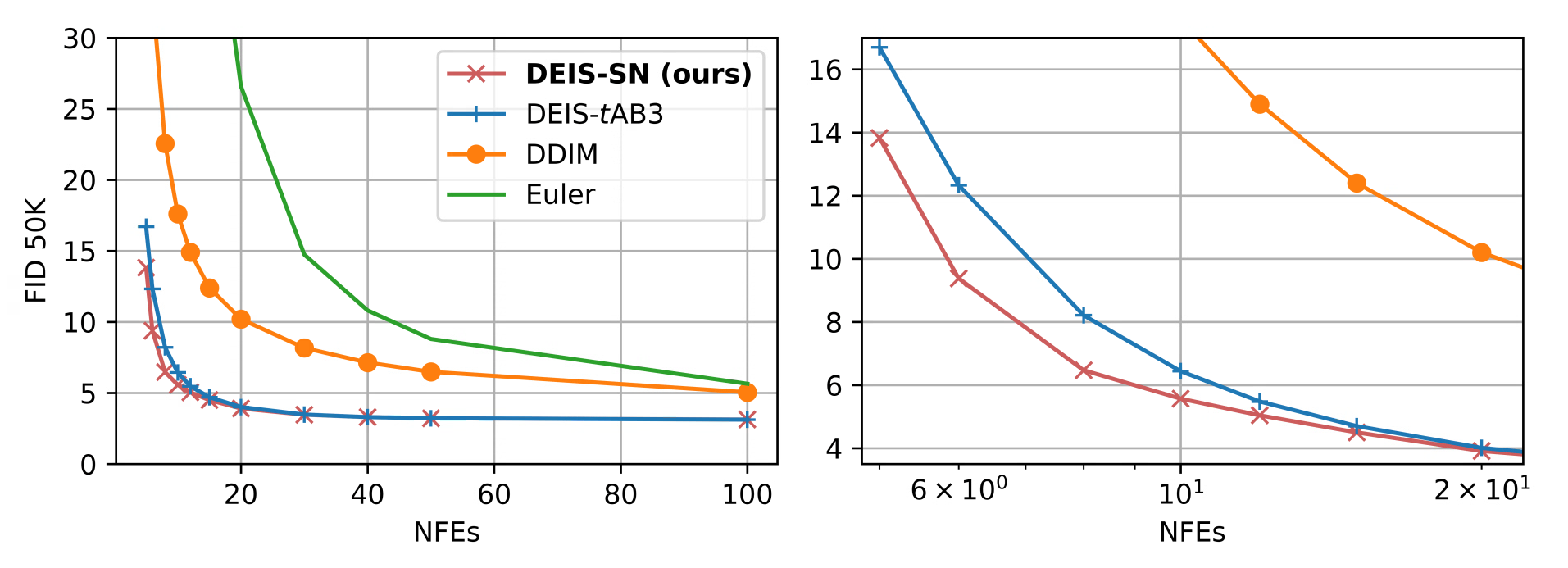
Figure 3: Left: FID 50K for CIFAR-10 against NFEs for different samplers on the same trained model. Right: zoomed in view of the left figure. DEIS-SN consistently outperforms DEIS at low NFEs.

We train the UNet architecture from [15] on CIFAR-10 [10] using the linear $\beta$ schedule [4] on noise prediction. We compare our approach to Euler integration of Eq. 4, DDIM [21] and DEIS-$t$AB3 (polynomial order $r=3$) [25]. DEIS-SN is identical to DEIS-$t$AB3 other than the choice of $K_{t}=1/\bar{s}_{\theta}(t)$ over $K_{t}=\sigma_{t}$. The average absolute score estimate $\bar{s}_{\theta}(t)$ is measured offline on a batch of 256 generations. For Euler and DDIM we use trailing linear time steps [11], whilst for DEIS we use trailing quadratic time $i\in\{0,\dots,N\}$, $t_{i}=(i/N)^{2}$. For full experimental details see Appendix A. A similar protocol was followed for LSUN-Church ($64\times 64$) experiments.

Fig. 3 shows for CIFAR-10, that at low NFEs, DEIS-SN provides a consistent FID improvement over vanilla DEIS. For higher NFEs, when the width of the intervals $[t_{i-1},t_{i}]$, and thus the integration error, is reduced, the benefit of DEIS-SN gradually disappears and DEIS-SN performs almost identically to vanilla DEIS. Both DDIM and Euler significantly underperform both DEIS approaches. Experimental results for LSUN-Church are shown in Appendix E.

Fig. 1 shows visual comparisons of vanilla DEIS and DEIS-SN at 5 NFEs. We see that DEIS-SN can better generate details (such as vehicle wheels). We note that generally generations are visually similar on a high level. This is because the difference between vanilla DEIS and DEIS-SN only occurs for $t$ near 0 (Fig. 2), i.e. the end of the generation/reverse process.

6 Conclusion

In this work we propose to extend the Diffusion Exponential Integrator Sampler (DEIS) with empirical score normalisation (DEIS-SN). Through our novel score-reparameterisation, we aim to further reduce integration error towards the end of the generation process by normalising the score estimate with the empirical average absolute value of previous score estimates. We validate our approach empirically on CIFAR-10 and LSUN-Church, showing that DEIS-SN is able to consistently outperform vanilla DEIS for low NFE generations in terms of FID 50k. We also show visual examples of DEIS-SN’s superiority.

In the future it would be interesting to extend this work to cover non-isotropic cases, where the score reparameterisation $\boldsymbol{K}_{t}$ is performed by a matrix, possibly in a transformed space such as the frequency domain [1, 5], to see if additional performance gains are to be had. Another possibility would be to parameterise $K_{t}$ and directly optimise it for better image quality at low NFEs.

Appendix A Additional Experimental Details

In order to perform sampling with our proposed method, and for comparison purposes, we trained a model to approximate the true score $\nabla_{\boldsymbol{x}_{t}}\log p(\boldsymbol{x}_{t})$ with a standard architecture and training procedure. We purposefully use a model with relatively small capacity to segregate the effects of sampling procedure and better score estimation [22, 7]. We train our score estimator in a discrete DDPM Ho et al. [4] setup with time-discretization granularity $N=1000$, $i\in\{0,\dots,N\}$, $t_{i}=i/N$, which is considered to be a standard in diffusion literature. As suggested by Ho et al. [4], we train the score estimator with the “simple loss” which is proven to be better at generation quality, as opposed to the true variational bound [9]. Again, as per Ho et al. [4], we do not directly estimate the score $\boldsymbol{s}_{\theta}$, but instead estimate the “noise-predictor” $\boldsymbol{\epsilon}_{\theta}$. Concretely, We optimize the following objective,

$$\mathbb{E}_{\boldsymbol{x}_{0}\sim p(\boldsymbol{x}_{0}),\ \boldsymbol{x}_{t}\sim p(\boldsymbol{x}_{t}|\boldsymbol{x}_{0}),\ i\sim\mathcal{U}\{1,N\},\ \epsilon\sim\mathcal{N}(0,I)}\left[||\boldsymbol{\epsilon}_{\theta}(\boldsymbol{x}_{t_{i}},t_{i})-\boldsymbol{\epsilon}||_{2}^{2}\right],$$ (6)

where $p(\boldsymbol{x}_{0})$ is the data distribution realized using our dataset, the forward noising conditional $p(\boldsymbol{x}_{t}|\boldsymbol{x}_{0})$ is from Eq. 1 and $t_{i}$ are timesteps. We use the standard “positional embeddings” for incorporating $t_{i}$ into the noise-estimator neural network. The $(a_{t},\sigma_{t})$ in Eq. 1 are chosen to be the standard “linear schedule” and variance-preserving formulation [22], i.e.

$$\textstyle a_{t}^{2}=\prod_{t^{\prime}=1}^{t}(1-\beta_{t^{\prime}}),\text{ and }\sigma_{t}=\sqrt{1-a_{t}^{2}}$$ (7)

where $\beta_{t}=\beta_{min}+(\beta_{max}-\beta_{min})\cdot t$ with $\beta_{min}=10^{-4}$ and $\beta_{max}=2\times 10^{-2}$. To obtain continuous time $a_{t}$ we employ simple linear interpolation as in [25]. We use the AdamW optimizer with learning rate $10^{-4}$ and no gradient clipping. We also use the standard process of using Exponential Moving Average (EMA) while training the network $\boldsymbol{\epsilon}_{\theta}$ using Eq. 6. We used a minibatch size of $128$ on each of $4$ GPUs, making the effective batch size $512$. We trained for $2000$ epochs on both CIFAR-10 [10] and LSUN-Church constituting $196k$ iterations and simply chose the final checkpoint. For faster training, we used mixed-precision training, which did not degrade any performance as per our experiments. The architecture of the U-Net used as $\boldsymbol{\epsilon}_{\theta}$ is taken exactly to be the standard architecture proposed in iDDPM [15], with a dropout rate of $0.3$. All our experiments are implemented using the diffusers library [23].

When generating samples for evaluation, we set the random seed to be the same value across all experiments. This allows a better comparison between different ODE sampling methods as different samplers will still follow similar trajectories (see Fig. 1).

Appendix B Mathematical Simplifications

We note that a number of simplifications/analytic results can be leveraged for DEIS, when applied specifically to the variance preserving process [4, 25],

$$\sigma_{t}^{2}=1-a_{t}^{2},\quad g_{t}^{2}=-2f_{t},\quad\Psi(t,s)=a_{t}/a_{s}.$$ (8)

Appendix C DEIS-SN Implementation Details

We follow Zhang and Chen [25]’s DEIS implementation closely for the most part. One minor difference is that we set $t_{0}=0$ rather than a small value such as $10^{-4}$. We find that for the samplers that we use this does not lead to any discontinuities/divide-by-zero errors, since no function is actually evaluated at $t=0$ (Eq. 5 uses a one-sided Riemann sum for numerical integration).

We find empirically that performance is improved by truncating $\bar{s}_{\theta}(t)$ slightly, close to $t=0$. This is possibly due to numerical instability from its rapid increase as $\sigma_{t}\rightarrow 0$. We simply set $\bar{s}_{\theta}(t)=\bar{s}_{\theta}(0.005)$ for $t<0.005$. We calculate $\bar{s}_{\theta}(t)$ by measuring the average absolute pixel values of $\boldsymbol{s}_{\theta}(\boldsymbol{x}_{t},t)$ at each time step using DEIS-$t$AB3 with 1000 NFEs (1000 uniform time steps) over a batch of 256 generations. This is done using a different random seed to the generations used for evaluation. We then use linear interpolation to obtain values over continuous time.

Appendix D More generation results

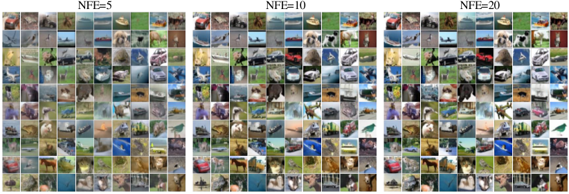
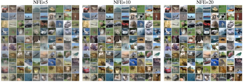
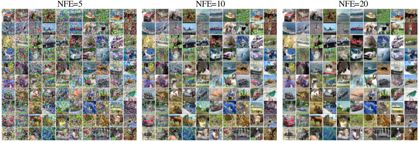
Figure 4: Visual comparison of unconditional samples for CIFAR10 generated (with same seed) at relatively low NFE for (top to bottom) DEIS-SN (Ours), DEIS, DDIM & Euler sampler.

Appendix E Results on LSUN-Church

We follow exactly same protocol except the UNet architecture, which in this case is adapted from [2]. The UNet in question has an attention resolution of only $16$ (unlike $16,8$ in CIFAR-10 model) and $2$ ResNet blocks (unlike $3$ in CIFAR-10 model). We also use a dropout of $0.1$ while training out LSUN-Church model. Below, in Fig. 5, we present the FID-vs-NFE curves similar to Fig. 1 in the main paper.

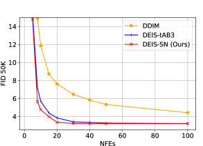
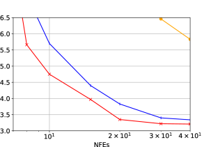
Figure 5: Left: FID 50K for LSUN-Church against NFEs for different samplers on the same trained model. Right: zoomed in view of the left figure. DEIS-SN consistently outperforms DEIS at low NFE regime.

References

- Das et al. [2023] Ayan Das, Stathi Fotiadis, Anil Batra, Farhang Nabiei, FengTing Liao, Sattar Vakili, Da shan Shiu, and Alberto Bernacchia. Image generation with shortest path diffusion. In International Conference on Machine Learning, 2023.
- Dhariwal and Nichol [2021] Prafulla Dhariwal and Alexander Nichol. Diffusion models beat gans on image synthesis. Advances in neural information processing systems, 34:8780–8794, 2021.
- Dockhorn et al. [2022] Tim Dockhorn, Arash Vahdat, and Karsten Kreis. Score-based generative modeling with critically-damped langevin diffusion. In International Conference on Learning Representations (ICLR), 2022.
- Ho et al. [2020] Jonathan Ho, Ajay Jain, and Pieter Abbeel. Denoising diffusion probabilistic models. In H. Larochelle, M. Ranzato, R. Hadsell, M.F. Balcan, and H. Lin, editors, Advances in Neural Information Processing Systems, volume 33, pages 6840–6851. Curran Associates, Inc., 2020.
- Hoogeboom and Salimans [2023] Emiel Hoogeboom and Tim Salimans. Blurring diffusion models. In The Eleventh International Conference on Learning Representations, 2023.
- Hoogeboom et al. [2022] Emiel Hoogeboom, Vıctor Garcia Satorras, Clément Vignac, and Max Welling. Equivariant diffusion for molecule generation in 3d. In International conference on machine learning, pages 8867–8887. PMLR, 2022.
- Karras et al. [2022] Tero Karras, Miika Aittala, Timo Aila, and Samuli Laine. Elucidating the design space of diffusion-based generative models. In S. Koyejo, S. Mohamed, A. Agarwal, D. Belgrave, K. Cho, and A. Oh, editors, Advances in Neural Information Processing Systems, volume 35, pages 26565–26577. Curran Associates, Inc., 2022.
- Karras et al. [2020] Tero Karras, Samuli Laine, Miika Aittala, Janne Hellsten, Jaakko Lehtinen, and Timo Aila. Analyzing and improving the image quality of StyleGAN. In Proc. CVPR, 2020.
- Kingma et al. [2021] Diederik Kingma, Tim Salimans, Ben Poole, and Jonathan Ho. Variational diffusion models. Advances in neural information processing systems, 2021.
- Krizhevsky et al. [2009] Alex Krizhevsky, Geoffrey Hinton, et al. Learning multiple layers of features from tiny images. 2009.
- Lin et al. [2023] Shanchuan Lin, Bingchen Liu, Jiashi Li, and Xiao Yang. Common diffusion noise schedules and sample steps are flawed. ArXiv, abs/2305.08891, 2023.
- Liu et al. [2023] Haohe Liu, Zehua Chen, Yi Yuan, Xinhao Mei, Xubo Liu, Danilo Mandic, Wenwu Wang, and Mark D Plumbley. Audioldm: Text-to-audio generation with latent diffusion models. arXiv preprint arXiv:2301.12503, 2023.
- Lu et al. [2022] Cheng Lu, Yuhao Zhou, Fan Bao, Jianfei Chen, Chongxuan LI, and Jun Zhu. Dpm-solver: A fast ode solver for diffusion probabilistic model sampling in around 10 steps. In S. Koyejo, S. Mohamed, A. Agarwal, D. Belgrave, K. Cho, and A. Oh, editors, Advances in Neural Information Processing Systems, volume 35, pages 5775–5787. Curran Associates, Inc., 2022.
- Lu et al. [2023] Cheng Lu, Yuhao Zhou, Fan Bao, Jianfei Chen, Chongxuan Li, and Jun Zhu. DPM-solver++: Fast solver for guided sampling of diffusion probabilistic models, 2023.
- Nichol and Dhariwal [2021] Alexander Quinn Nichol and Prafulla Dhariwal. Improved denoising diffusion probabilistic models. In Marina Meila and Tong Zhang, editors, Proceedings of the 38th International Conference on Machine Learning, volume 139 of Proceedings of Machine Learning Research, pages 8162–8171. PMLR, 18–24 Jul 2021.
- Poole et al. [2022] Ben Poole, Ajay Jain, Jonathan T Barron, and Ben Mildenhall. Dreamfusion: Text-to-3d using 2d diffusion. arXiv preprint arXiv:2209.14988, 2022.
- Rombach et al. [2022] Robin Rombach, Andreas Blattmann, Dominik Lorenz, Patrick Esser, and Björn Ommer. High-resolution image synthesis with latent diffusion models. In Proceedings of the IEEE/CVF conference on computer vision and pattern recognition, pages 10684–10695, 2022.
- Salimans and Ho [2022] Tim Salimans and Jonathan Ho. Progressive distillation for fast sampling of diffusion models. In International Conference on Learning Representations, 2022.
- Salimans et al. [2017] Tim Salimans, Andrej Karpathy, Xi Chen, and Diederik P. Kingma. Pixelcnn++: A pixelcnn implementation with discretized logistic mixture likelihood and other modifications. In ICLR, 2017.
- Sohl-Dickstein et al. [2015] Jascha Sohl-Dickstein, Eric Weiss, Niru Maheswaranathan, and Surya Ganguli. Deep unsupervised learning using nonequilibrium thermodynamics. In Francis Bach and David Blei, editors, Proceedings of the 32nd International Conference on Machine Learning, volume 37 of Proceedings of Machine Learning Research, pages 2256–2265, Lille, France, 07–09 Jul 2015. PMLR.
- Song et al. [2021] Jiaming Song, Chenlin Meng, and Stefano Ermon. Denoising diffusion implicit models. In International Conference on Learning Representations, 2021.
- Song et al. [2021] Yang Song, Jascha Sohl-Dickstein, Diederik P Kingma, Abhishek Kumar, Stefano Ermon, and Ben Poole. Score-based generative modeling through stochastic differential equations. In International Conference on Learning Representations, 2021.
- von Platen et al. [2022] Patrick von Platen, Suraj Patil, Anton Lozhkov, Pedro Cuenca, Nathan Lambert, Kashif Rasul, Mishig Davaadorj, and Thomas Wolf. Diffusers: State-of-the-art diffusion models. https://github.com/huggingface/diffusers, 2022.
- Watson et al. [2021] Daniel Watson, William Chan, Jonathan Ho, and Mohammad Norouzi. Learning fast samplers for diffusion models by differentiating through sample quality. In International Conference on Learning Representations, 2021.
- Zhang and Chen [2023] Qinsheng Zhang and Yongxin Chen. Fast sampling of diffusion models with exponential integrator. In The Eleventh International Conference on Learning Representations, 2023.
- Zhang et al. [2023] Qinsheng Zhang, Molei Tao, and Yongxin Chen. gDDIM: Generalized denoising diffusion implicit models. In The Eleventh International Conference on Learning Representations, 2023.
- Zheng et al. [2023] Hongkai Zheng, Weili Nie, Arash Vahdat, Kamyar Azizzadenesheli, and Anima Anandkumar. Fast sampling of diffusion models via operator learning. In International Conference on Machine Learning, 2023.