A Knowledge Compilation Take
on Binary Polynomial Optimization

Abstract

The Binary Polynomial Optimization (BPO) problem is defined as the problem of maximizing a given polynomial function over all binary points. The main contribution of this paper is to draw a novel connection between BPO and the problem of finding the maximal assignment for a Boolean function with weights on variables. This connection allows us to give a strongly polynomial algorithm that solves BPO with a hypergraph that is either $\beta$-acyclic or with bounded incidence treewidth. This result unifies and significantly extends the known tractable classes of BPO. The generality of our technique allows us to deal also with extensions of BPO, where we enforce extended cardinality constraints on the set of binary points, and where we seek $k$ best feasible solutions. We also extend our results to the significantly more general problem where variables are replaced by literals. Preliminary computational results show that the resulting algorithms can be significantly faster than current state-of-the-art.

Key words: Binary Polynomial Optimization; Knowledge Compilation; Boolean function

1 Introduction

In Binary Polynomial Optimization (BPO), we are given a hypergraph $H=(V,E)$, a profit function $p\from E\to\Q$, and our goal is to find some $x\in\{0,1\}^{V}$ that attains:

$$\max_{x\in\{0,1\}^{V}} \sum_{e\in E}p(e)\prod_{v\in e}x(v).$$ (BPO)

BPO is strongly NP-hard, as even the case where all the monomials have degree equal to 2 has this property [25]. Nevertheless, its generality and wide range of applications attract a significant amount of interest in the optimization community. A few examples of applications can be found in classic operations research, computer vision, communication engineering, and theoretical physics [2, 5, 41, 34, 28, 37]. To the best of our knowledge, four main polynomially solvable classes of BPO have been identified so far. These are instances such that: (i) the objective function is supermodular (see Chapter 45 in [40]); (ii) the primal treewidth of $H$, denoted by $\ptw{H}$, is bounded by $\log(\operatorname{poly}(|V|,|E|))$ [16, 33, 4]; (iii) $H$ is a cycle hypergraph [19]; (iv) $H$ is $\beta$-acyclic [20]. This last result generalizes prior tractability results about Berge-acyclic and $\gamma$-acyclic instances [22, 9] and kite-free $\beta$-acyclic instances [23]. Most of the techniques used to obtain the above tractability results either exploit directly the combinatorial nature of the problem, or are based on the linearization of the polynomials which allows for a subsequent polyhedral approach [21].

The main contribution of this paper is to draw a novel connection between BPO and the problem of performing algebraic model counting over the $(\max,+)$ semiring on some Boolean function [31]. We associate a Boolean function and a weight function to each BPO such that optimal solutions of the original BPO are in one to one correspondence with the optimal solutions of the Boolean function. This Boolean function can be encoded as a Conjunctive Normal Form (CNF) formula whose underlying structure is very close to the structure of the original BPO problem, allowing us to leverage many known tractability results on CNF formulas to BPO such as bounded treewidth CNF formulas [38] or $\beta$-acyclic formulas [12] (see [11, Chapter 3] for a survey). More interestingly, the tractability of algebraic model counting for CNF formulas is usually proven in two steps: first, one computes a small data structure which represents every satisfying assignment of the CNF formula in a factorized yet tractable form, as in [7], and for which we can find the optimal value in optimal time [31, 6]. This data structure can be seen as a syntactically restricted Boolean circuit, which have extensively been studied in the field of Knowledge Compilation [18]. Our connection actually shows that all feasible points of a tractable BPO instance and their value can be efficiently represented in such circuits. This enables us to transfer also other known tractability results to the setting of BPO. For example, by working directly on the Boolean circuit, we can not only prove that broad classes of BPO can be solved in polynomial time but also that we can solve BPO instances in these classes together with cardinality constraints or find the $k$ best solutions.

In the remainder of the introduction we present our complexity results. We remark that these complexity results constitute just the tip of the iceberg of what our novel connection can achieve. We begin by stating our first result for BPO, and we refer the reader to Section 3 for the definitions of $\beta$-acyclicity and of incidence treewidth of a hypergraph $H$, which we denote by $\itw{H}$.

Theorem 1 (Tractability of BPO).

There is a strongly polynomial time algorithm to solve the BPO problem, provided that $H$ is $\beta$-acyclic, or the incidence treewidth of $H$ is bounded by $\log(\operatorname{poly}(|V|,|E|))$.

Theorem 1 implies and unifies the known tractable classes (ii), (iii), (iv). To see that (ii) is implied, it suffices to note that $\ptw{H}\geq 2\itw{H}$. We observe that this bound can be very loose, as in fact the hypergraph with only one edge containing all $n$ vertices has $\ptw{H}=n-1$ and $\itw{H}=1$. Hence, Theorem 1 significantly extends (ii).

The generality of our approach allows us to significantly extend Theorem 1 in several directions. The first extension enables us to consider a constrained version of BPO, with a more general feasible region. Namely, we consider feasible regions consisting of binary points that satisfy extended cardinality constraints of the form

$$\sum_{v\in V}x(v)\in S,$$

for some $S\subseteq[n]$ where $n=|V|,$ and where the set $S$ is given as part of the input. Note that extended cardinality constraints are quite general and extend several classes of well-known inequalities, like cardinality constraints and modulo constraints. To the best of our knowledge, there are only two classes of constrained BPO that are known to be solvable in polynomial time. In these two classes, the feasible region consists of (a) binary points satisfying cardinality constraints $l\leq\sum_{v\in V}x_{v}\leq u$, and $E$ is nested [13] or $|E|=2$ [14]; or (b) binary points satisfying polynomial constraints

$$\sum_{f\subseteq e_{i}}p^{i}(f)\prod_{v\in f}x(v)\geq 0,\qquad i=1,\dots,m,$$

where, for $i=1,\dots,m$, $e_{i}\subseteq V$ and $p^{i}\from 2^{e_{i}}\to\Q$, and it is assumed that the primal treewidth of $(V,E\cup\{e_{1},\dots,e_{m}\})$ is bounded by $\log(\operatorname{poly}(|V|,|E|,m))$ [43, 33, 4].

Our second extension allows us to consider a different overarching goal. In fact, we consider the problem of finding $k$ best solutions to the optimization problem, rather than only one optimal solution. We are not aware of any known result in this direction.

Our third extension concerns the objective function of the problem. Namely, we consider the objective function obtained from the one of BPO by replacing variables with literals:

$$\sum_{e\in E}p(e)\prod_{v\in e}\sigma_{e}(v),$$

where, for each $e\in E$, $\sigma_{e}$ is a mapping (given in input) with $\sigma_{e}(v)\in\{x(v),\ 1-x(v)\}$. We refer to this class of problems as Binary Polynomial Optimization with Literals, abbreviated BPO${}_{\text{L}}$. This optimization problem is at the heart of the area of research known as pseudo-Boolean optimization in the literature, and we refer the reader to [5] for a thorough survey. In the unconstrained case, i.e., the feasible region consists of $\{0,1\}^{V}$, it is known that BPO${}_{\text{L}}$ can be solved in polynomial time if $H$ is $\beta$-acyclic [29]. This result, as well as the tractability of (a) above, is implied by our most general statement, the extension of Theorem 1, given below.

Theorem 2.

There is a strongly polynomial time algorithm to find $k$ best feasible solutions to the BPO${}_{\text{L}}$ with extended cardinality constraints, provided that $H$ is $\beta$-acyclic, or the incidence treewidth of $H$ is bounded by $\log(\operatorname{poly}(|V|,|E|))$.

A key feature of our approach is that it also leads to practically efficient algorithms for BPO. Preliminary computational results show that the resulting algorithms can be significantly faster than current state-of-the-art on some structured instances.

Organization of the paper.

The paper is organized as follows: we first draw a connection between solving a BPO problem and finding optimal solutions of a Boolean function for a given weight function in Section 2. We then explain in Section 3 how the Boolean function can be encoded as a CNF formula that preserves the structure of the original BPO problem. Section 4 explains how such CNF can be turned into Boolean circuits known as d-DNNF where finding optimal solutions is tractable. Section 5 explores generalizations of BPO and show how the d-DNNF representation allows for solving these generalizations by directly transforming the circuit. Finally, Section 6 shows some encouraging preliminaries experiment. The structure of the paper is summarized in Figure 1.

Figure 1: Structure of the paper.

2 Binary Polynomial Optimization and

In this section, we detail a connection between solving a BPO problem and finding optimal solutions of a Boolean function for a given weight function.

Binary Polynomial Optimization Problem.

Our first goal is to redefine Binary Polynomial Optimization problems using hypergraphs. A hypergraph $H$ is a pair $(V,E)$, where $V$ is a finite set of vertices $V$ and $E\subseteq 2^{V}$ is a set of edges. Given a hypergraph $H=(V,E)$ and a profit function $p\from E\to\Q$, the Binary Polynomial Optimization problem for $(H,p)$ is defined as finding an optimal solution $x^{*}\in\{0,1\}^{V}$ to the following maximization problem: $\max_{x\in\{0,1\}^{V}}P_{(H,p)}(x)$ where $P_{(H,p)}$ is the polynomial defined as $P_{(H,p)}(x)=\sum_{e\in E}p(e)\prod_{v\in e}x(v)$. We denote this problem as $\BPO$. The value $P_{(H,p)}(x^{*})$ is called the optimal value of $\BPO$.

.

A closely related notion is the notion of . Let $X$ be a finite set of variables. We denote by $\{0,1\}^{X}$ the set of assignments on variables $X$ to Boolean values, that is, the set of mappings $\tau\from X\to\{0,1\}$. A Boolean function on variables $X$ is a subset of assignments $f\subseteq\{0,1\}^{X}$. An assignment $\tau\in f$ is said to be a satisfying assignment of $f$. A weight function $w$ on variables $X$ is a mapping $w:X\times\{0,1\}\to\Q$. Given $\tau\in\{0,1\}^{X}$, we let $w(\tau)=\sum_{x\in X}w(x,\tau(x))$. Given a Boolean function $f$ on variables $X$, we let $w(f)=\max_{\tau\in f}w(\tau)$. That is

$$w(f)=\max_{\tau\in f}\sum_{x\in X}w(x,\tau(x)).$$

This value can be seen as a form of Algebraic Model Counting on the $(\Q\cup\{-\infty\},\max,+,-\infty,0)$ semiring, which is most of the time $\NP$-hard to compute but for which we know some tractable classes [31]. Given a Boolean function $f$ and a weight function $w$, the $(f,w)$ is defined as the problem of computing an optimal solution $\tau^{*}\in f$, that is, an assignment $\tau^{*}\in\{0,1\}^{X}$ such that $w(\tau^{*})=w(f)$.

BPO as .

There is a pretty straightforward connections between the BPO problem and the , which is based on the notion of multilinear sets introduced by Del Pia and Khajavirad in [21]. Given a hypergraph $H=(V,E)$, the multilinear set $f_{H}$ of $H$ is the Boolean function on variables $X\cup Y$ where $X=\{x_{v}\}_{v\in V}$ and $Y=\{y_{e}\}_{e\in E}$ such that $\tau\in f_{H}$ if and only if for every $e\in E$, $\tau(y_{e})=\prod_{v\in e}\tau(x_{v})$.

Moreover, given a profit function $p\from E\to\Q$, we define a weight function $w_{p}\from X\cup Y\times\{0,1\}\to\Q$ as:

• for every $v\in V$ and $b\in\{0,1\}$, $w_{p}(x_{v},b)=0$,

• for every $e\in E$ and $b\in\{0,1\}$, $w_{p}(y_{e},b)=b\times p(e)$.

In the next lemma, we show that the BPO instance $(H,p)$ is equivalent to the $(f_{H},w_{p})$, in the sense that any $\tau\in f_{H}$ can naturally be mapped to a feasible point $x_{\tau}\in\{0,1\}^{V}$ whose value is the weight of $\tau$. More formally:

Lemma 1.

For every $\tau\in f_{H}$, we have $P_{(H,p)}(x_{\tau})=w_{p}(\tau)$ where the mapping $x_{\tau}\in\{0,1\}^{V}$ is defined as $x_{\tau}(v)=\tau(x_{v})$ for every $v\in V$.

Proof.

Recall that by definition, $\tau\in f_{H}$ if and only if $\tau(y_{e})=\prod_{v\in e}\tau(x_{v})$. We have:

$$w_{p}(\tau) =\sum_{v\in V}w_{p}(x_{v},\tau(x_{v}))+\sum_{e\in E}w_{p}(y_{e},\tau(y_{e}))$$

$$=\sum_{v\in V}0+\sum_{e\in E}\tau(y_{e})p(e)\text{ by definition of $w_{p}$}$$

$$=\sum_{e\in E}p(e)\prod_{v\in e}\tau(x_{v})\text{ since $\tau\in f_{H}$}$$

$$=\sum_{e\in E}p(e)\prod_{v\in e}x_{\tau}(x_{v})\text{ by definition of $x_{\tau}$}$$

$$=P_{(H,p)}(x_{\tau}).$$

∎

Theorem 3.

Let $(H,p)$ be an instance of BPO. The set of optimal solutions of $\BPO$ is equal to $\{x_{\tau^{*}}\mid\tau^{*}\text{ is an optimal solution of }(f_{H},w_{p})\}$.

Proof.

First of all, observe that given $x\in\{0,1\}^{V}$, there exists a unique $\tau\in f_{H}$ such that $x=x_{\tau}$. Indeed, we define $\tau(x_{v})=x(v)$ and $\tau(y_{e})=\prod_{v\in e}x(v)$. It is readily verified that $\tau\in f_{H}$ and that $x=x_{\tau}$. Let $x^{*}$ be an optimal solution of $\BPO$ and let $\tau$ be such that $x^{*}=x_{\tau}$. We claim that $\tau$ is an optimal solution of $(f_{H},w_{p})$. Indeed, let $\tau^{\prime}\in f_{H}$. By Lemma 1, $w_{p}(\tau^{\prime})=P_{(H,p)}(x_{\tau^{\prime}})$ and $P_{(H,p)}(x_{\tau^{\prime}})\leq P_{(H,p)}(x^{*})$ since $x^{*}$ is optimal. Moreover, $P_{(H,p)}(x^{*})=w_{p}(\tau)$ by Lemma 1 again. Hence $w_{p}(\tau^{\prime})\leq w_{p}(\tau)$. In other words, $\tau$ is an optimal solution of $(f_{H},w_{p})$. Now let $\tau^{*}$ be an optimal solution of $(f_{H},w_{p})$. By a symmetric reasoning, we show that $x_{\tau^{*}}$ is an optimal solution of $\BPO$. Indeed, for every $x\in\{0,1\}^{V}$, if $\tau\in f_{H}$ is such that $x=x_{\tau}$; by Lemma 1, we have $P_{(H,p)}(x)=w_{p}(x_{\tau})\leq w_{p}(\tau^{*})=P_{(H,p)}(x_{\tau^{*}})$. ∎

This connection is at the heart of our main technique for solving BPO problems in this paper: if $H$ is such that $w_{p}(f_{H})$ is known to be tractable, then we can use Theorem 3 to leverage these results on Boolean function directly to BPO. We study in the next section some Boolean function for which the is tractable.

3 Encoding BPO as CNF formulas

In the previous section, we have established a relation between a BPO problem $(H,p)$ and the problem $(f_{H},w_{p})$ of finding an optimal solution to the Boolean function $f_{H}$ for the weight function $p$. This connection is merely a rewriting of the original problem and, without any detail on how $f_{H}$ is encoded, it does not provide any insight on the complexity of solving BPO. In this section, we explore encodings of $f_{H}$ in Conjunctive Normal Form (CNF), which is a very generic way of encoding Boolean functions. This is also the usual input of SAT solvers. We compare the structure of $H$ and the structure of our CNF encodings. In Section 4, we will use this structure to discover tractable classes of BPO.

CNF formulas.

Given a set of variables $X$, a literal over $X$ is an element of the form $x$ or $\neg x$ for some $x\in X$. Given an assignment $\tau\in\{0,1\}^{X}$, we naturally extend it to literals by defining $\tau(\neg x)=1-\tau(x)$. A clause $C$ over $X$ is a set of literals over $X$. We denote by $\var{C}$ the set of variables appearing in $C$. An assignment $\tau$ satisfies a clause $C$ if and only if there exists a literal $\ell\in C$ such that $\tau(\ell)=1$. A Conjunctive Normal Form formula $F$ over $X$, CNF formula for short, is a set of clauses over $X$. We denote by $\var{F}$ the set of variables appearing in $F$. An assignment $\tau$ satisfies $F$ if and only if it satisfies every clause in $F$. Hence a CNF formula over $X$ naturally induces a Boolean function over $X$, which consists of the set of satisfying assignments of $F$.

A first encoding.

In this section, we fix a hypergraph $H=(V,E)$ and a profit function $p$. From Theorem 3, one can think of the BPO instance $(H,p)$ as a Boolean function that expresses the structure of the polynomial objective function through constraints of the form $y_{e}=\prod_{v\in e}x_{v}$, for all $e\in E$. From a logical point of view, it corresponds to the logical equivalence $y_{e}\iff\bigwedge_{v\in e}x_{v}$, for all $e\in E$. In fact, given $e\in E$, $y_{e}=1$ if and only if all the variables present in that specific monomial represented by $e$ have value equal to 1, i.e., $x_{v}=1$ for all $v\in e$. Let us now consider some $e\in E$, and see more in detail how the two implications of the above if and only if are expressed both from an integer optimization point of view and from a more logical point of view.

On the one hand, we must encode that if $x_{v}=1$ for all $v\in e$, then $y_{e}=1$. In the integer optimization approach, the typical single constraint that is added in this case is $\sum_{v\in e}x_{v}-y_{e}\leq|e|-1$. The most straightforward way of encoding this as a CNF formula is as $y_{e}\vee\bigvee_{v\in e}\neg x_{v}$. In fact, if $x_{v}=1$ for all $v\in e$ then, for the formula to be satisfied, we need to have $y_{e}=1$.

On the other hand, we also want to model that if $y_{e}=1$ then each $v\in e$ must satisfy $x_{v}=1$ too. In the optimization community this is usually done by adding the constraints $y_{e}\leq x_{v}$ for every $v\in e$. The easiest way to do with a CNF formula is by adding the clause $\neg y_{e}\vee x_{v}$ for each $v\in e$. If $y_{e}=1$, then the clause can only be satisfied if $x_{v}=1$.

The above discussion motivates the following definition: $F_{H}$ is the CNF formula on variables $X\cup Y$ having the following clauses for every $e\in E$:

• $R_{e}=y_{e}\vee\bigvee_{v\in e}\neg x_{v}$,

• and for every $v\in e$, $L_{e,v}=\neg y_{e}\vee x_{v}$.

Example 1.

Let us consider the multilinear expression $-3x_{1}x_{2}x_{3}+4x_{4}x_{5}+5x_{2}x_{3}x_{4}x_{5}x_{6}$. The typical hypergraph that represents it is $G=(V,E)$ with $V=\{v_{1},v_{2},v_{3},v_{4},v_{5},v_{6}\}$ and $E$ containing only three edges $\{v_{1},v_{2},v_{3}\}$, $\{v_{4},v_{5}\}$, $\{v_{2},v_{3},v_{4},v_{5},v_{6}\}$.

Now let us construct its CNF encoding, which involves 9 variables and 13 clauses. Specifically it is:

$$(\neg y_{e_{1}}\vee x_{v_{1}})\wedge(\neg y_{e_{1}}\vee x_{v_{2}})\wedge(\neg y_{e_{1}}\vee x_{v_{3}})\wedge(\neg x_{v_{1}}\vee\neg x_{v_{2}}\vee\neg x_{v_{3}}\vee y_{e_{1}})\wedge$$

$$(\neg y_{e_{2}}\vee x_{v_{4}})\wedge(\neg y_{e_{2}}\vee x_{v_{5}})\wedge(\neg x_{v_{4}}\vee\neg x_{v_{5}}\vee y_{e_{2}})\wedge$$

$$(\neg y_{e_{3}}\vee x_{v_{2}})\wedge(\neg y_{e_{3}}\vee x_{v_{3}})\wedge(\neg y_{e_{3}}\vee x_{v_{4}})\wedge(\neg y_{e_{3}}\vee x_{v_{5}})\wedge(\neg y_{e_{3}}\vee x_{v_{6}})\wedge$$

$$(\neg x_{v_{2}}\vee\neg x_{v_{3}}\vee\neg x_{v_{4}}\vee\neg x_{v_{5}}\vee\neg x_{v_{6}}\vee y_{e_{3}}).$$

The corresponding hypergraph is depicted in Figure 3. $\diamond$

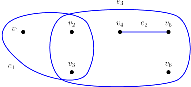
Figure 2: Hypergraph $G$ representing $x_{1}x_{2}x_{3}+x_{4}x_{5}+x_{2}x_{3}x_{4}x_{5}x_{6}$.

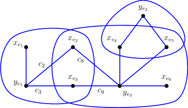
Figure 3: Hypergraph representing first CNF construction.

$F_{H}$ is an actual encoding as witnessed by the following:

Lemma 2.

For every hypergraph $H$, the satisfying assignments of $F_{H}$ are exacly $f_{H}$.

Proof.

$F_{H}$ is the conjunction of the usual clause encoding of constraints of the form $y_{e}\Leftrightarrow\bigwedge_{v\in e}x_{v}$, where $R_{e}$ encodes $\bigwedge_{v\in e}x_{v}\Rightarrow y_{e}$ and $L_{e,v}$ encodes $y_{e}\Rightarrow x_{v}$ and hence $\bigwedge_{v\in e}L_{e,v}$ corresponds to $y_{e}\Rightarrow\bigwedge_{v\in e}\tau(x_{v})$. Hence $\tau$ satisifes $F_{H}$ if and only if $\tau(y_{e})\Leftrightarrow\bigwedge_{v\in e}\tau(x_{v})$, which is equivalent to say that $\tau(y_{e})=\prod_{v\in e}x_{v}$, that is, $\tau\in f_{H}$. ∎

3.1 A CNF encoding preserving treewidth

We now turn our attention to proving that some structure of hypergraph $H$ can be found in the CNF encoding $F_{H}$. One of the most studied structures that is known to give interesting tractability both for CNF formulas and for BPO is the case of bounded treewidth hypergraphs. This class has a long history in the SAT solving community, where the tractability of SAT on CNF having bounded treewidth has been established in several independent work such as [1, 26], later generalized in [42]. In the BPO community, several work establish the tractability for bounded treewidth [43, 33, 4].

Treewidth.

Let $G=(V,E)$ be a graph. A tree decomposition $\calT=(T,(B_{t})_{t\in V_{T}})$ is a tree $T=(V_{T},E_{T})$ together with a labeling $B$ of its vertices, such that the two following properties hold:

• Covering: For every $e\in E$, there exists $t\in V_{T}$ such that $e\subseteq B_{t}$.

• Connectedness: For every $v\in V$, $\{t\in V_{T}\mid v\in B_{t}\}$ is connected in $T$.

An element $B_{t}$ of $B$ is called a bag of $\calT$. The treewidth of $\calT$ is defined as $\tw{G}[\calT]=\max_{t\in B_{t}}|B_{t}|-1$, that is, the size of the biggest bag minus $1$. The treewidth of $G$ is defined to be the smallest possible width over every tree decomposition of $G$, that is, $\tw{G}=\min_{\calT}\tw{G}[\calT]$.

Two notions of treewidth can be defined for hypergraphs depending on the underlying graph considered. Recall that A graph $G=(V,E)$ is a hypergraph such that for every $e\in E$, $|e|=2$. Given a hypergraph $H=(V,E)$, we associate two graphs to it. The primal graph $\prim[H]$ of $H$ is defined as the graph whose vertex set is $V$ and edge set is $\{\{u,v\}\mid u\neq v,\exists e\in E,\ u,v\in e\}$. Intuitively, the primal graph is obtained by replacing every edge of $H$ by a clique. The incidence graph $\inc[H]$ of $H$ is defined as the bipartite graph whose vertex set is $V\cup E$ and the edge set is $\{\{v,e\}\mid v\in V,e\in E,v\in e\}$. Similarly, the primal graph $\prim[F]$ of a CNF formula $F$ is the graph whose vertices are the variables of $F$ and such that there is an edge between variables $x$ and $y$ if and only if there is a clause $C\in F$ such that $x,y\in\var{C}$. The incidence graph $\inc[F]$ of $F$ is the bipartite graph on vertices $\var{F}\cup F$ such that there is an edge between a variable $x$ and a clause $C$ of $F$ if and only if $x\in\var{C}$.

Given a hypergraph $H$, its primal treewidth $\ptw{H}$ is defined as the treewidth of its primal graph, that is $\ptw{H}=\tw{\prim[H]}$, while its incidence treewidth $\itw{H}$ is defined as the treewidth of its incidence graph, that is $\itw{H}=\tw{\inc[H]}$. The primal treewidth of $F$ is defined to be $\tw{\prim[F]}$. The incidence treewidth of $F$ is defined to be $\tw{\inc[F]}$.

We now prove a relation between the incidence treewidth of $F_{H}$ and of the incidence treewidth of $H$:

Lemma 3.

For every $H=(V,E)$, we have $\itw{F_{H}}\leq 2\cdot(1+\itw{H})$.

Proof.

The proof is based on the following observation. Let $G^{\prime}=(V^{\prime},E^{\prime})$ be the graph obtained from $\inc[H]$ as follows: we introduce for every edge $e\in E$ a vertex $y_{e}$ that is connected to $e$ and to every $v\in e$. Clearly, $e$ and $y_{e}$ have the same neighborhood in $G^{\prime}$ and $\inc[H]$ can be obtained by contracting $e$ and $y_{e}$ for every $e\in E$. Such a transformation is known as a modules contraction in graph theory and one can easily prove that the treewidth of $G^{\prime}$ is at most $2(1+\itw{H})$ (see Lemma 11 in the Appendix for a full proof). Now, one can get $\inc[F_{H}]$ by renaming every vertex $v$ of $G^{\prime}$ into $x_{v}$ and every vertex $e$ into $R_{e}$ and by splitting the edge $\{y_{e},x_{v}\}$ of $G^{\prime}$ with a node $L_{e,v}$. Hence $\inc[F_{H}]$ is obtained from $G^{\prime}$ by splitting edges, an operation that preserves treewidth (see Lemma 10 in Appendix for details). In other words, $\itw{F_{H}}\leq\tw{G^{\prime}}\leq 2(1+\itw{H})$. ∎

We observe here that bounded incidence treewidth also captures a class of hypergraphs that is known to be tractable for BPO: the class of cycle hypergraphs [19]. We define a cycle hypergraph as a hypergraph $H=(V,E)$ such that $E=\{e_{0},\dots,e_{n-1}\}$ and $e_{i}\cap e_{j}\neq\emptyset$ if and only if $j=i+1\mod n$. We remark that this definition is slightly more general than the one in [19]. While the primal treewidth of a cycle hypergraph can be arbitrarely large (since an edge of size $k$ induces a $k$-clique in the primal graph and hence treewidth larger than $k$), the incidence treewidth of cycle hypergraphs is $2$.

Lemma 4.

For every cycle hypergraph $H=(V,E)$, we have $\itw{H}\leq 2$.

Proof.

We give a tree decomposition $T$ for $\inc[H]$ of width $2$. We start by introducing $n$ bags $B_{0},\dots,B_{n-1}$ connected by a path such that $B_{0}=\{e_{0},e_{1}\}$ and $B_{i}=\{e_{0},e_{i},e_{i+1}\}$ for $1\leq i<n-1$ and $B_{n-1}=\{e_{0},e_{n-1}\}$. We connect to $B_{i}$ one bag $\{e_{i},e_{i+1\mod n},v\}$ for every $v\in e_{i}\cap e_{(i+1)\mod n}$ and one bag $\{e_{i},v\}$ for every $v\in e_{i}\setminus(e_{i-1\mod n}\cup e_{i+1\mod n})$. We claim that this tree decomposition, which clearly has width $2$, is a tree decomposition of $\inc[H]$. Indeed, every edge of $\inc[H]$ is of the form $(e_{i},v)$. Moreover, since $H$ is a cycle hypergraph:

• Either $v\in e_{i-1\mod n}$ in which case the edge $(e_{i},v)$ is covered by the bag $\{e_{i-1\mod n},e_{i},v\}$ connected to $B_{i-1}$.

• Either $v\in e_{i+1\mod n}$ in which case the edge $(e_{i},v)$ is covered by the bag $\{e_{i+1\mod n},e_{i},v\}$ connected to $B_{i}$.

• Or $v\in e_{i}\setminus(e_{i-1\mod n}\cup e_{i+1\mod n})$ in which case the edge $(e_{i},v)$ is covered by the bag $\{e_{i},v\}$ connected to $B_{i}$.

Hence every edge of $\inc[H]$ is covered by $T$. It remains to show that the connectedness requirement holds. Let $w$ be a vertex of $\inc[H]$. Either $w$ is an edge $e_{i}$ of $H$ or it is a vertex of $H$. Let us start from examining the case where $w$ is an edge of $H$. If $i=0$, the subgraph induced by $w$ is connected since $e_{0}$ appears in every $B_{i}$ and every other bag is connected to some $B_{i}$. If $w=e_{i}$, for $i>0$, then $e_{i}$ appears only in $B_{i}$, $B_{i+1}$ or in bags connected to $B_{i}$ or $B_{i+1}$. Hence the subgraph of $T$ induced by $e_{i}$ is connected. Now $w$ may be a vertex $v\in V$. It is easy to see however that $v$ appears in at most one bag of the tree decomposition and is hence connected. ∎

3.2 A CNF encoding preserving $\beta$-acyclicity

Several generalizations of graph acyclicity have been introduced for hypergraphs [24], but in this paper we will be interested in the notion of $\beta$-acyclicity. A good overview of notions of acyclicities for hypergraphs can be found in [8]. They are particularly interesting since both CNF and BPO are tractable on $\beta$-acyclic hypergraphs.

Let $H=(V,E)$ be a hypergraph. For a vertex $v\in V$, we denote by $E(v)=\{e\in E\mid v\in e\}$ the set of edges containing $v$. A nest point of $H$ is a vertex $v\in V$ such that $E(v)$ is ordered by inclusion, that is, for any $e,f\in E(v)$ either $e\subseteq f$ or $f\subseteq e$. $H$ is $\beta$-acyclic if there exists an ordering $(v_{1},\dots,v_{n})$ of $V$ such that for every $i\leq n$, $v_{i}$ is a nest point of $H\setminus\{v_{1},\dots,v_{i-1}\}$, where $H\setminus W$ is the hypergraph with vertex set $V\setminus W$ and edge set $\{e\setminus W\mid e\in E\}$. Such ordering is called a $\beta$-elimination order. A hypergraph is $\beta$-acyclic if and only if it has a $\beta$-elimination order. For a CNF formula, the hypergraph $H(F)$ of $F$ is the hypergraph whose vertices are $\var{F}$ and edges are $\var{C}$ for every $C\in F$. A CNF formula is said to be $\beta$-acyclic if and only if $H(F)$ is $\beta$-acyclic.

It has been recently proven that the BPO problem is tractable when its underlying hypergraph is $\beta$-acyclic [20]. This result is akin to known tractability for $\beta$-acyclic CNF formulas [12]. To connect both results, it is tempting to use the CNF encoding $F_{H}$ from previous section. However, one can construct a $\beta$-acyclic hypergraph $H$ where $F_{H}$ is not $\beta$-acyclic. This can actually be seen on the example from Figure 3, which is $\beta$-acyclic since $\{v_{1},\dots,v_{6}\}$ is a $\beta$-elimination order but $F_{H}$, depicted on 3, is not $\beta$-acyclic, since it contains, for example, the $\beta$-cycle formed by the vertices $\{x_{v_{2}},y_{e_{1}},x_{v_{3}},y_{e_{2}}\}$ and edges $\{c_{2},c_{3},c_{9},c_{8}\}$.

We can nevertheless design a CNF encoding of $f_{H}$ for $H=(V,E)$ that preserves $\beta$-acyclicity, as follows: given a total order $\prec$ on $V$, we let $F_{H}^{\prec}$ be a CNF on variables $X\cup Y$ with $X=(x_{v})_{v\in V}$ and $Y=(y_{e})_{e\in E}$ having clauses:

• for every $e\in E$, there is a clause $R_{e}=y_{e}\vee\bigvee_{v\in e}\neg x_{v}$,

• for every $e\in E$ and $v\in e$, there is a clause $L^{\prec}_{v,e}=\neg y_{e}\vee x_{v}\vee\bigvee_{w\in e,v\prec w}\neg x_{w}$.

The CNF encoding from Example 1 following the variable order $\{v_{1},\dots,v_{6}\}$ and its hypergraph are depicted on Figure 4. It is easy to see that this hypergraph is $\beta$-acyclic.

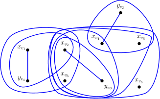
$$\scriptsize\displaystyle(\neg y_{e_{1}}\vee x_{v_{1}})\wedge(\neg y_{e_{1}}\vee x_{v_{2}}\vee\neg x_{v_{1}})\wedge$$

$$\scriptsize\displaystyle(\neg y_{e_{1}}\vee x_{v_{3}}\vee\neg x_{v_{1}}\vee\neg x_{v_{2}})\wedge$$

$$\scriptsize\displaystyle(\neg x_{v_{1}}\vee\neg x_{v_{2}}\vee\neg x_{v_{3}}\vee y_{e_{1}})\wedge(\neg y_{e_{2}}\vee x_{v_{4}})\wedge$$

$$\scriptsize\displaystyle(\neg y_{e_{2}}\vee x_{v_{5}}\vee\neg x_{v_{4}})\wedge(\neg x_{v_{4}}\vee\neg x_{v_{5}}\vee y_{e_{2}})\wedge$$

$$\scriptsize\displaystyle(\neg y_{e_{3}}\vee x_{v_{2}})\wedge(\neg y_{e_{3}}\vee x_{v_{3}}\vee\neg x_{v_{2}})\wedge$$

$$\scriptsize\displaystyle(\neg y_{e_{3}}\vee x_{v_{4}}\vee\neg x_{v_{2}}\vee\neg x_{v_{3}})\wedge$$

$$\scriptsize\displaystyle(\neg y_{e_{3}}\vee x_{v_{5}}\vee\neg x_{v_{2}}\vee\neg x_{v_{3}}\vee x_{v_{4}})\wedge$$

$$\scriptsize\displaystyle(\neg y_{e_{3}}\vee x_{v_{6}}\vee\neg x_{v_{2}}\vee\neg x_{v_{3}}\vee\neg x_{v_{4}}\vee\neg x_{v_{5}})\wedge$$

$$\scriptsize\displaystyle(\neg x_{v_{2}}\vee\neg x_{v_{3}}\vee\neg x_{v_{4}}\vee\neg x_{v_{5}}\vee\neg x_{v_{6}}\vee y_{e_{3}}).$$

Figure 4: Hypergraph and CNF for $\beta$-acyclic preserving encoding.

As before, the satisfying assignments of $F_{H}^{\prec}$ are the same as $f_{H}$ since $R_{e}$ encodes the constraint $\bigwedge_{v\in V}x_{v}\Rightarrow y_{e}$ and $\bigwedge_{v\in e}L_{v,e}^{\prec}$ encodes $y_{e}\Rightarrow\bigwedge_{v\in e}x_{v}$.

Lemma 5.

For every hypergraph $H=(V,E)$ and order $\prec$ on $V$, the satisfying assignments of $F_{H}^{\prec}$ are exactly $f_{H}$.

This encoding now preserves $\beta$-acyclicity when the right order is used:

Lemma 6.

Let $H=(V,E)$ be a $\beta$-acyclic hypergraph and $\prec$ be a $\beta$-elimination order for $H$. Then $F_{H}^{\prec}$ is $\beta$-acyclic.

Proof.

We claim that $(y_{e_{1}},\dots,y_{e_{m}},x_{v_{1}},\dots,x_{v_{n}})$ is a $\beta$-elimination order of $H(F_{H}^{\prec})$, where $V=\{v_{1},\dots,v_{n}\}$ with $v_{i}\prec v_{j}$ for any $i<j$ and $E=\{e_{1},\dots,e_{m}\}$ is an arbitrary order on $E$. First we observe that for any $e\in E$, $y_{e}$ is a nest point of $H(F_{H}^{\prec})$. Indeed, $y_{e}$ is exactly in $R_{e}$ and $L_{v,e}$ for every $v\in e$. The fact that $y_{e}$ is a nest point follows from the fact that $\var{L_{v,e}}\subseteq\var{L_{w,e}}$ if $w\prec v$ and that $\var{L_{v,e}}\subseteq\var{R_{e}}$ by definition.

Hence, one can eliminate $y_{e_{1}},\dots,y_{e_{m}}$ from $H(F_{H}^{\prec})$. Let $H^{\prime}$ be the resulting hypergraph. Observe that the vertices of $H^{\prime}$ are $\{x_{v_{1}},\dots,x_{v_{n}}\}$. Our goal is to show that $(x_{v_{1}},\dots,x_{v_{n}})$ is a $\beta$-elimination order for $H^{\prime}$ and we will do it using the fact that $(v_{1},\dots,v_{n})$ is a $\beta$-elimination order of $H$. In order to ease the comparison between the two hypergraphs, we consider $H^{\prime}$ to be a hypergraph on vertices $v_{1},\dots,v_{n}$ by simply renaming $x_{v_{i}}$ to $v_{i}$.

Now, let $V_{i}=\{v_{1},\dots,v_{i}\}$. We claim that if $f$ is an edge of $H^{\prime}$ containing $v_{i+1}$ then $f\setminus V_{i}$ is an edge of $H\setminus V_{i}$. Indeed, either $f$ is an edge of $H^{\prime}$ corresponding to a clause $R_{e}$. In this case, $f=\var{R_{e}}\setminus\{y_{e}\}$ since $y_{e}$ has been removed in $H^{\prime}$ and hence $f=e$, by definition of $R_{e}$. Hence $f$ is an edge of $H$, that is, $f\setminus V_{i}$ is an edge of $H\setminus V_{i}$.

Otherwise, $f$ is of the form $\var{L_{v,e}^{\prec}}\setminus\{y_{e}\}$ for some $e\in E$ and $v\in e$, that is, $f=e\cap\{w\in V\mid v\preceq w\}$. Since $v_{i+1}$ is in $f$, it means that $v\prec v_{i+1}$ or $v=v_{i+1}$. Hence $f\setminus V_{i}=e\setminus V_{i}$.

Now it is easy to see that $v_{i+1}$ is a nest point of $H^{\prime}\setminus V_{i}$. Indeed, let $e,f$ be two edges of $H^{\prime}\setminus V_{i}$ that contains $v_{i+1}$. By definition, $e=e^{\prime}\setminus V_{i}$ and $f=f^{\prime}\setminus V_{i}$ for some edges $e^{\prime},f^{\prime}$ of $H^{\prime}$. However, $e$ and $f$ are also edges of $H\setminus V_{i}$. By definition, $v_{i+1}$ is a nest point of $H\setminus V_{i}$. Hence $e\subseteq f$ or $f\subseteq e$. In any case, it means that $v_{i+1}$ is a nest point of $H^{\prime}\setminus V_{i}$ and hence, $(v_{1},\dots,v_{n})$ is a $\beta$-elimination order of $H^{\prime}$. ∎

4 Solving BPO using Knowledge Compilation

The complexity of finding an optimal solution for a $(f,w)$ given a Boolean function $f$ and a weight function $w$ depends on the way $f$ is represented in the input. If $f$ is given in the input as a CNF formula, then deciding $w(f)=0$ is $\NP$-hard, since even deciding whether $f$ is satisfiable is $\NP$-hard. Now, if $f$ is given on the input as a truth table, that is, as the list of its satisfying assignments, then it is straightforward to compute $w(f)$ in polynomial time by just computing explicitly $w(\tau)$ for every $\tau\in f$ and return the largest value. This algorithm is polynomial in the size of the truth table, hence, computing $w(f)$ in this setting is tractable. However, one can easily observe that this algorithm is polynomial time only because the input was given in a very explicit and non-succinct manner. The domain of Knowledge Compilation [30] has focused on the study of the representations of Boolean functions, together with their properties, and, more generally, on analysing the tradeoff between the succinctness and the tractability of representations of Boolean functions. An overview presenting these representations and what is tractable on them can be found in the survey by Darwiche and Marquis [18].

In this paper, we are interested in the deterministic Decomposable Negation Normal Form representation, d-DNNF for short, a representation introduced in [17]. This data structure has two advantages for our purposes. On the one hand, given a Boolean function $f$ represented as a d-DNNF $C$ and a weight function $w$, one can find an optimal solution for $(f,w)$ in polynomial time in the size of $C$ [6, 31]. On the other hand, d-DNNF can succinctly encode CNF formulas having bounded incidence treewidth or $\beta$-acyclic CNF formulas [12, 7].

A Negation Normal Form circuit (NNF circuit for short) $C$ on variables $X$ is a labeled directed acyclic graph (DAG) such that:

• $C$ has a specific node $v$ called the output of $C$ and denoted by $\out$.

• Every node of $G$ of in-degree $0$ is called an input of $C$ and is labeled by either $0$, $1$ or a literal $\ell$ over $X$.

• Every other node of $G$ is labeled by either $\wedge$ or $\vee$. Let $v$ be such a node and $w$ be such that there is an oriented edge from $w$ to $v$ in $C$. We say that $w$ is an input of $v$ and we denote by $\inputs$ the set of inputs of $v$.

Given a node $v$ of $C$, we denote by $\var{v}$ the subset of $X$ containing the variables $y$ such that there is path from an input labeled by $y$ or $\neg y$ to $v$. Each node of $C$ computes a Boolean function $f_{v}\subseteq 2^{\var{v}}$ inductively defined as:

• If $v$ is an input labeled by $0$ (respectively $1$), then $f_{v}=\emptyset$ (respectively $f_{v}=2^{\emptyset}$)

• If $v$ is an input labeled by $x$ (respectively $\neg x$) then $f_{v}$ is the Boolean function over $\{x\}$ that contains exactly the one assignment mapping $x$ to $1$ (respectively to $0$)

• If $v$ is labeled by $\vee$ then $\tau\in f_{v}$ if and only if there exists $w\in\inputs$ such that $\tau|_{\var{w}}\in f_{w}$. In other words, $f_{v}=\bigvee_{w\in\inputs}f_{w}$.

• If $v$ is labeled by $\wedge$ then $\tau\in f_{v}$ if and only if for every $w\in\inputs$ we have $\tau|_{\var{w}}\in f_{w}$. In other words, $f_{v}=\bigwedge_{w\in\inputs}f_{w}$.

The Boolean function $f_{C}$ computed by $C$ over $X$ is defined as $f_{\out}\times 2^{X\setminus\var{\out}}$. The size of $C$ is defined as the number of edges in the circuit and denoted by $|C|$.

x	y	z
0	1	0
0	1	1
1	0	0
1	1	0
1	1	1

Figure 5: A deterministic DNNF and the Boolean function it computes. Observe that each $\wedge$-node mentions disjoint variables ($x$ or $y$ or $z$) and the each $\vee$-node is deterministic: the bottom one because they differ on the value of $z$ and the top one because they differ on the value assigned to $x$ and $y$.

A $\wedge$-node $v$ is said to be decomposable if for every $w,w^{\prime}\in\inputs$, $\var{w}\cap\var{w^{\prime}}=\emptyset$. An NNF circuit is a Decomposable Negation Normal Form circuit, DNNF for short, if every $\wedge$-node of the circuit is decomposable.

A $\vee$-node $v$ is said to be deterministic if for every $\tau\in f_{v}$, there exists a unique $w\in\inputs$ such that $\tau|_{\var{w}}\in f_{w}$. A deterministic Decomposable Negation Normal Form circuit, d-DNNF for short, is a DNNF where every $\vee$-node is deterministic. An example of d-DNNF is given on Figure 5.

Observe that in a d-DNNF circuit, the following identities hold:

• If $v$ is a $\vee$-node then $f_{v}=\biguplus_{w\in\inputs}\big{(}f_{w}\times 2^{\var{v}\setminus\var{w}}\big{)}$, where $\uplus$ denotes disjoint union;

• If $v$ is a $\wedge$-node then $f_{v}=\bigtimes_{w\in\inputs}f_{w}$.

These identities allow to design efficient dynamic programming schemes on d-DNNF circuits. In this paper, we will be mostly interested in such dynamic programming scheme to compute optimal solutions to . The next theorem is a direct consequence of [6, Theorem 1] but, since it is stated in a slightly different framework there, we also provide a proof sketch. In this paper, the size of numbers, denoted by $\operatorname{size}(\cdot)$, is the standard one in mathematical programming, and is essentially the number of bits required to encode such numbers. We refer the reader to [39] for a formal definition of size.

Theorem 4.

Let $(f,w)$ be a and $C$ a d-DNNF such that $f=f_{C}$. We can find an optimal solution $\tau^{*}\in f$ for $w$ in strongly polynomial time, i.e., with $O(\operatorname{poly}(|C|))$ arithmetic operations on numbers of size $\operatorname{poly}(size(w))$.

Proof (sketch)..

The idea is to compute inductively, for each node $v$ of $C$, an optimal solution $\tau_{v}^{*}$ of the problem $(f_{v},w)$, that is, a solution $\tau_{v}^{*}\in f_{v}$ such that $w(\tau_{v}^{*})$ is maximal. We recall that $w(\tau_{v}^{*})$ is equal to $\sum_{x\in\var{v}}w(\tau_{v}^{*},\tau_{v}^{*}(x))$. If $v$ is a leaf labeled by literal $\ell$, then $f_{v}$ contains exactly one assignment, which is hence optimal by definition.

Now let $v$ be an internal node of $C$ and let $v_{1},\dots,v_{k}$ be its input. Assume that for each $v_{i}$, an optimal solution $\tau_{v_{i}}^{*}$ of $(f_{v_{i}},w)$ has been precomputed. If $v$ is a $\wedge$-node, then we have that $f_{v}=\bigtimes_{i=1}^{k}f_{v_{i}}$, by the fact that the circuit is decomposable. It can be easily verified that $\tau^{*}_{v}:=\bigtimes_{i=1}^{k}\tau^{*}_{v_{i}}$ is an optimal solution of $f_{v}$ which proves the induction step in this case. Otherwise, $v$ must be a $\vee$-node and in this case, $f_{v}=\bigcup_{i=1}^{k}f_{v_{i}}\times\{0,1\}^{\var{v}\setminus\var{v_{i}}}$. An optimal solution $\sigma_{i}^{*}$ for $\{0,1\}^{\var{v}\setminus\var{v_{i}}}$ can be obtained by taking $\sigma_{i}^{*}(x)=b\in\{0,1\}$ if $w(x,b)\geq w(x,1-b)$ for every $x\in\var{v}\setminus\var{v_{i}}$. In this case $\tau^{*}_{v_{i}}\times\sigma^{*}_{i}$ is an optimal solution of $f_{v_{i}}\times\{0,1\}^{\var{v}\setminus\var{v_{i}}}$. Finally, observe that an optimal solution of $f_{v}$ has to be an optimal solution for $f_{v_{i}}\times\{0,1\}^{\var{v}\setminus\var{v_{i}}}$ for some $i$. Hence, $\tau_{v}^{*}=\argmax_{i=1}^{k}w(\tau_{v_{i}}^{*}\times\sigma_{i}^{*})$ is an optimal solution of $f_{v}$.

At each gate, we have to compare at most $O(|C|)$ numbers, each of size $\operatorname{poly}(\operatorname{size}(w))$, to decide which optimal solution to take. Since we are doing this at most once per gate, we have an algorithm that computes an optimal solution of $f=f_{C}$ with $\operatorname{poly}(|C|)$ arithmetic operations on number of size at most $\operatorname{poly}(\operatorname{size}(w))$. ∎

Theorem 4 becomes interesting for our purpose since it is known that both $\beta$-acyclic CNF formulas [12] and bounded incidence treewidth CNF formulas [7] can be represented as polynomial size d-DNNF:

Theorem 5 ([12]).

Let $F$ be a $\beta$-acyclic CNF formula having $n$ variables and $m$ clauses. One can construct a d-DNNF $C$ of size $\operatorname{poly}(n,m)$ in time $\operatorname{poly}(n,m)$ such that $f_{C}$ is the set of satisfying assignments of $F$.

Theorem 6 ([7]).

Let $F$ be a CNF formula having $n$ variables, $m$ clauses and incidence treewidth $t$. One can construct a d-DNNF $C$ in time $2^{t}\operatorname{poly}(n,m)$ of size $2^{t}\operatorname{poly}(n,m)$ such that $f_{C}$ is the set of satisfying assignments of $F$.

As a consequence, we can represent the multilinear set of a BPO problem $(H,p)$ with a polynomial size d-DNNF if the incidence treewidth of $H$ is bounded:

Theorem 7.

Let $H=(V,E)$ and $t=\itw{H}$. The multilinear set $f_{H}$ of $H$ can be computed by a d-DNNF of size $2^{O(t)}\operatorname{poly}(|V|,|E|)$ that can be constructed in time $2^{O(t)}\operatorname{poly}(|V|,|E|)$.

Proof.

We construct $F_{H}$ from $H$ in time $\operatorname{poly}(|E|,|V|)$. It has $n=|V|+|E|$ variables, $m\leq|E|(1+|V|)$ clauses and incidence treewidth at most $2(t+1)$ by Lemma 3. Hence the construction follows by applying Theorem 6 to $F_{H}$. ∎

Symmetrically, if $H$ is $\beta$-acyclic we get:

Theorem 8.

Let $H=(V,E)$ be a $\beta$-acyclic hypergraph. The multilinear set $f_{H}$ of $H$ can be computed by a d-DNNF of size $\operatorname{poly}(|V|,|E|)$ that can be constructed in time $\operatorname{poly}(|V|,|E|)$.

In particular, Theorem 1 follows from Theorem 4 together with Theorem 8 for the first part and with Theorem 7 for the last part.

5 Beyond BPO

In this section, we show the versatility of our circuit-based approach by showing how we can use it to solve optimization problems beyond BPO.

5.1 Adding Cardinality Constraints

We start by focusing on solving BPO problems that are combined, for example, with cardinality or modulo constraints, that is, a BPO problem with additional constraints on the value of $\sum_{v\in V}x(v)$. In this section, we will be interested in the extended cardinality constraints that we define as constraints of the form $\sum_{v\in V}x(v)\in S$, for some $S\subseteq[n]$ where $n=|V|$.

Our approach is based on a transformation of the d-DNNF so that they only accept assignments whose number of variables set to $1$ is constrained. The key result is the following one:

Theorem 9.

Let $C$ be a d-DNNF on variables $Z$ and let $X\subseteq Z$ with $p=|X|$. One can construct a d-DNNF $C^{\prime}$ in time $O(\operatorname{poly}(|C|))$ and of size $O(\operatorname{poly}(|C|))$ such that there exists nodes $r_{0},\dots,r_{p}$ in $C^{\prime}$ with $f_{r_{i}}=f_{C}\cap B_{i}(X,Z)$ where $B_{i}(X,Z)=\{\tau\in\{0,1\}^{Z}\mid\sum_{x\in X\cap Z}\tau(x)=i\}$ for $i\in[p]$.

Proof.

Recall that each node $v$ of $C$ computes a Boolean function $f_{v}$ on $\var{v}$ inductively defined in Section 2. The main idea of the proof is to construct $C^{\prime}$ by introducing $p+1$ copies $v^{(0)},\dots,v^{(p)}$ for every node $v$ of $C$ and plug them together so that $f_{v^{(i)}}$ computes $f_{v}\cap B_{i}(X,\var{v})$. Observe that if $|\var{v}\cap X|<p$ then for $|\var{v}\cap X|<j\leq p$, $f_{v}\cap B_{j}(X,\var{v})=\emptyset$, so we do not really need to introduce a copy $v^{(j)}$. However, in order to minimize the number of cases to consider in the induction, we introduce $p$ copies for each $v$, regardless of $|\var{v}\cap X|$.

To make the transformation easier to perform, we first assume that $C$ has been normalized so that for every $\vee$-node $v$ and input $w$ of $v$, we have $\var{v}=\var{w}$ (a property known as smoothness [18]) and such that every $\wedge$-node has at most two inputs. It is known that one can normalize $C$ in polynomial time (see [11, Theorem 1.61] for details).

We now construct from $C$ a new circuit $C^{\prime}$ of size at most $3p^{2}|C|$ that will have the following property: for each node $v$ of $C$, there exists $v^{(0)},\dots,v^{(p)}$ in $C^{\prime}$ such that $v^{(i)}$ computes $f_{v}\cap B_{i}(X,\var{v})$. The construction of $C^{\prime}$ is done by induction on the size of $C$.

We start with the base case where $C$ contains exactly one node, which is then necessarely an input $v$. If $v$ is labeled by $0$, $1$, $y$ or $\neg y$ with $y\notin X$ or by $\neg x$ with $x\in X$ then we add an input node $v^{(0)}$ with the same label as $v$ and introduce $0$-input $v^{(1)},\dots,v^{(p)}$. If $v$ is an input node of $C$ labeled by $x\in X$, we introduce an input labeled by $x$ as $v^{(1)}$ and let $v^{(0)},v^{(2)},\dots,v^{(p)}$ be $0$-inputs. It can readily be verified that for every previous case, that is, for every case where $v$ is an input, then $f_{v}\cap B_{i}(X,\var{v^{(i)}})$ is the same as $f_{v^{(i)}}$ for every $i\in[n]$. Moreover, $|C^{\prime}|\leq p=3p^{2}|C|$ in this case, which respects the induction hypothesis.

We now proceed to the inductive step. Let $v$ be node of $C$ that has outdegree $0$ and let $C_{0}$ be the circuit obtained by removing $v$ from $C$. By induction, we can construct a circuit $C^{\prime}_{0}$ of size at most $3p^{2}|C_{0}|=3p^{2}|C|-3p^{2}$, such that for every node $w$ of $C_{0}$ – that is for every node of $C$ that is different from $v$, there exists $w^{(0)},\dots,w^{(p)}$ in $C_{0}^{\prime}$ such that $w^{(i)}$ computes $f_{w}\cap B_{i}(X,\var{w})$. Observe that $w$ computes the same function in $C_{0}$ or in $C$ since we have removed a gate of outdegree $0$ that is hence not used in the computation of any other $f_{w}$. Hence, to construct $C^{\prime}$, it is enough to add new vertices $v^{(0)},\dots,v^{(p)}$ in $C_{0}^{\prime}$ such that $v^{(i)}$ computes $f_{v}\cap B_{i}(X,\var{v})$. We now explain how to do it by adding at most $3p^{2}$ nodes in $C_{0}^{\prime}$, resulting in a circuit $C^{\prime}$ that will respect the induction hypothesis.

We start with the case where $v$ is a $\vee$-node. Let $w_{1},\dots,w_{k}$ be the inputs of $v$. For every $i\in[p]$, we create a new $\vee$-node $v^{(i)}$ and add it to $C_{0}^{\prime}$ and connect it to the nodes $w_{j}^{(i)}$ of $C_{0}^{\prime}$ for every $j\leq k$, where $w_{j}^{(i)}$ is the node of $C_{0}^{\prime}$ computing $f_{w_{j}}\cap B_{i}(X,\var{w_{j}})$ given by induction.

We claim that $v^{(i)}$ computes $f_{v}\cap B_{i}(X,\var{v})$. Indeed, since $C$ is smooth, $\var{w_{j}}=\var{v}$. Hence we have: $f_{v^{(i)}}=\bigcup_{j=1}^{k}f_{w_{j}^{(i)}}=\bigcup_{j=1}^{k}(f_{w_{j}}\cap B_{i}(X,\var{v}))=f_{v}\cap B_{i}(X,\var{v})$, which is the induction hypothesis. Moreover $C^{\prime}$ is obtained from $C_{0}^{\prime}$ by adding at most $p$ new gates, hence $|C^{\prime}|=|C_{0}^{\prime}|+p\leq 3p^{2}(|C|-1)+p\leq 3p^{2}|C|$.

We now deal with the case where $v$ is a $\wedge$-node of $C$ with inputs $w_{1},w_{2}$ (recall that $C$ has been normalized so that $\wedge$-nodes have two inputs). We construct $C^{\prime}$ by adding, for every $i\leq p$, a new $\vee$-node $v^{(i)}$ in $C_{0}^{\prime}$. Moreover, for every $(a,b)\in[p]^{2}$ such that $a+b=i$, we add a new node $\wedge$-node $v_{a,b}$.

Let $w_{1}^{(a)}$ and $w_{2}^{(b)}$ be the nodes in $C_{0}^{\prime}$ computing $f_{w_{1}}\cap B_{a}(X,\var{w})$ and $f_{w_{2}}\cap B_{b}(X,\var{w})$ respectively. We add the edge $w_{1}^{(a)}\rightarrow v_{a,b}$ and $w_{2}^{(b)}\rightarrow v_{a,b}$ in $C_{0}^{\prime}$, that is, $v_{a,b}$ has now $w_{1}^{(a)}$ and $w_{2}^{(b)}$ as inputs. Moreover, for every $a,b$ such that $a+b=i$, we add the edge $v_{a,b}\rightarrow v^{(i)}$, that is, the input of $v^{(i)}$ are the set of nodes $v_{a,b}$ such that $a+b=i$. We claim that $v^{(i)}$ computes $f_{v}\cap B_{i}(X,\var{v})$.

It is readily verified that $f_{v^{(i)}}=\bigcup_{(a,b)\mid a+b=i}f_{w_{1}^{(a)}}\times f_{w_{2}^{(b)}}$. By induction, this is equal to $\bigcup_{(a,b)\mid a+b=i}(f_{w_{1}}\cap B_{a}(X,\var{w_{1}}))\times(f_{w_{2}}\cap B_{b}(X,\var{w_{2}})$. Now, it is easy to see that this set is included in $(f_{w_{1}}\times f_{w_{2}})\cap B_{i}(X,\var{w})=f_{v}\cap B_{i}(X,\var{v})$. To see the other inclusion, consider $\tau\in f_{v}\cap B_{i}(X,\var{v})$. By definition, $\tau=\tau_{1}\times\tau_{2}$ with $\tau_{1}\in f_{w_{1}}$ and $\tau_{2}\in f_{w_{2}}$. Moreover, $i=\sum_{x\in X\cap\var{v}}\tau(x)=\sum_{x\in X\cap\var{w_{1}}}\tau(x)+\sum_{x\in X\cap\var{w_{2}}}\tau(x)$. Let $a^{\prime}=\sum_{x\in X\cap\var{w_{1}}}\tau(x)$ and $b^{\prime}=\sum_{x\in X\cap\var{w_{2}}}\tau(x)$. We have $a^{\prime}+b^{\prime}=i$ and $\tau_{1}=\tau|_{\var{w_{1}}}\in B_{a^{\prime}}(X,\var{w_{1}})$ and $\tau_{2}=\tau|_{\var{w_{2}}}\in B_{b^{\prime}}(X,\var{w_{2}})$. Hence $\tau=\tau_{1}\times\tau_{2}\in(f_{w_{1}}\cap B_{a^{\prime}}(X,\var{w_{1}}))\times(f_{w_{2}}\cap B_{b^{\prime}}(X,\var{w_{2}})$ with $a^{\prime}+b^{\prime}=i$. This is enough to conclude that

$$\bigcup_{(a,b)\mid a+b=i}(f_{w_{1}}\cap B_{a}(X,\var{w_{1}}))\times(f_{w_{2}}\cap B_{b}(X,\var{w_{2}})=f_{v}\cap B_{i}(X,\var{v}).$$

Finally, observe that $C^{\prime}$ is obtained from $C_{0}^{\prime}$ by adding $3$ edges for each $v_{a,b}$ node, that is, at most $3p^{2}$ edges. Hence $|C^{\prime}|\leq|C_{0}^{\prime}|+3p^{2}\leq 3p^{2}(|C|-1)+3p^{2}=3p^{2}|C|$, which concludes the induction.

Now let $C^{\prime}$ be the circuit obtained from $C$ by doing the previously describe transformation. Let $r=\out[C]$. Then by construction, there exists $r^{(i)}$ in $C^{\prime}$ computing $f_{C}\cap B_{i}(X,Z)$ and $C^{\prime}$ is of size at most $3p^{2}|C|=\operatorname{poly}(p)|C|$. Moreover, it is straightforward to see that this construction can be down in polynomial time by induction on the circuit which concludes the proof. ∎

We will be mostly interested in the following corollary:

Corollary 1.

Let $S\subseteq[p]$ and $C$ be a d-DNNF on variables $Z$ and $X\subseteq Z$ with $|X|=p$. We can construct a d-DNNF $C^{\prime}$ of size $\operatorname{poly}(|C|)$ in time $\operatorname{poly}(|C|)$ such that $f_{C^{\prime}}=f_{C}\cap B_{S}(X,Z)$ where $B_{S}(X,Z)=\bigcup_{i\in S}B_{i}(X,Z)$.

Proof.

Let $C_{0}$ be the circuit given by Theorem 9 and define $C^{\prime}$ by adding a new $\vee$-node $r$ that is connected to $r^{(i)}$ for every $i\in S$ in $C_{0}$. It is readily verified that $f_{r}=f_{C}\cap B_{S}(X,Z)$. ∎

Now Corollary 1 allows to solve any $(f,w)$ with an additional constraint $\sum_{x\in X}\tau(x)\in S$ for $S\subseteq[p]$ and $X\subseteq Z$ in polynomial time if $f$ is given as a d-DNNF and has variable set $Z$. Indeed, this optimization problem can be reformulated as the problem $(f\cap B_{S}(X,Z),w)$. By Corollary 1, $f\cap B_{S}(X,Z)$ can be represented by a d-DNNF of size $\operatorname{poly}(|C|)$ that we can use to compute $w(f\cap B_{S}(X))$ in $\operatorname{poly}(|C|)$ by Theorem 4. Hence, the previous discussion and Theorems 7 and 8 imply:

Theorem 10.

Let $H=(V,E)$ be a hypergraph, $p$ a profit function and $S\subseteq V$. We can solve the optimization problem

$$\max_{x\in\{0,1\}^{V}} P_{(H,p)}(x)$$

s.t. $$\sum_{x\in V}x(v)\in S$$

in time $\operatorname{poly}(|V|,|E|)$ if $H$ is $\beta$-acyclic and in time $2^{O(t)}\operatorname{poly}(|V|,|E|)$ where $t$ is the incidence treewidth of $H$.

Proof.

We explain it for the $\beta$-acyclic case, the other case being completely symmetric. By Theorem 8, there is a d-DNNF $C$ computing $f_{H}$ of size $\operatorname{poly}(|V|,|E|)$. Recall that $f_{H}$ is defined on variables $X=(x_{v})_{v\in V}$ and $Y=(y_{e})_{e\in E}$. By Corollary 1, there is a d-DNNF $C^{\prime}$ computing $f_{H}\cap B_{S}(X,X\cup Y)$, that is, the set of $\tau\in f_{H}$ such that $\sum_{v\in V}\tau(x_{v})\in S$. By Lemma 1, $f_{H}\cap B_{S}(X,X\cup Y)$ is isomorphic to $\mathcal{B}=\{\sigma\in\{0,1\}^{V}\mid\sum_{v\in V}\sigma(v)\in S\}$ and this isomorphism preserves the weights. Hence $w_{p}(f_{H}\cap B_{S}(X,X\cup Y))$ is the same as $\max_{\sigma\in\mathcal{B}}P_{(H,p)}(\sigma)$, which is the value we are looking for. Hence we can compute the desired optimal value in $\operatorname{poly}(|C^{\prime}|)$, that is, $\operatorname{poly}(|V|,|E|)$. ∎

In particular, BPO problems with cardinality or modulo constraints are tractable on $\beta$-acyclic hypergraphs and bounded incidence treewidth hypergraphs since a conjunction of such constraints can easily be encoded as a single extended cardinality constraints. We insist here on the fact that the modulo and cardinality constraint have to be over every variable of the polynomial, or the structure of the resulting hypergraph would be affected.

Finally, we observe that the construction from Theorem 9 can be generalized to solve problem with one knapsack constraint. A knapsack constraint is a constraint of the form $L\leq\sum_{v\in V}c_{v}x(v)\leq U$ where $L,U,c_{v}\in\Z$. The construction is more expensive that the previous one as it will provide an algorithm whose complexity is polynomial in $M=|V|\cdot\max_{v\in V}|c_{v}|$, which is not polynomial in the input size if the integer values $c_{v}$ are assumed to be binary encoded. Indeed, we know that for any $x\in\{0,1\}^{V}$, $\sum_{v\in V}c_{v}x(v)$ will be between $-M$ and $M$. Hence, we can modify the construction of Theorem 9 so that $C^{\prime}$ has a node $r^{(i)}$ for every $i\in[-M;M]$ and such that $f_{r^{(i)}}=f_{C}\cap\{\tau\in\{0,1\}^{V}\mid\sum c_{v}x(v)=i\}$.

5.2 Top-$k$ for BPO

We now turn our attention to the problem of computing $k$ best solutions for a given $k$. This task is natural when there is more than one optimal solution and one wants to explore them in order to find a solution that is more suitable to the user’s needs than the one found by the solver. Formally, a top-$k$ set for a BPO instance $(H,p)$ is a set $K=\{\sigma_{1},\dots,\sigma_{k}\}\subseteq\{0,1\}^{V}$ of size $k$ such that $P_{(H,p)}(\sigma_{1})\geq\dots\geq P_{(H,p)}(\sigma_{k})$ and such that for every $\sigma\notin K$, $P_{(H,p)}(\sigma)\leq P_{(H,p)}(\sigma_{k})$. We observe that a top-$k$ set for a BPO instance may not be unique, as two distinct $\sigma,\sigma^{\prime}$ may have the same value under $P_{(H,p)}$. The top-$k$ problem asks for outputting a top-$k$ set given a BPO instance $(H,p)$ and $k\in\mathbb{N}$ on input.

We similarly define the top-$k$ problem for a $(f,w)$. It turns out that finding a top-$k$ set for $f$ when $f$ is given as a d-DNNF $C$ is tractable. The proof is very similar to the one of Theorem 4 but instead of constructing an optimal solution $\tau_{v}^{*}$ of $f_{v}$ for each gate $v$, we construct a top-$k$ set $K_{v}$ for $f_{v}$. We can build such top-$k$ sets in a bottom up fashion by observing that if the circuit has been normalized as in Theorem 9, we have that if $v$ is a $\vee$-gate with input $v_{1},\dots,v_{p}$, then a top-$k$ set of $f_{v}$ can be found by taking a top-$k$ set of $\bigcup_{i=1}^{p}K_{v_{i}}$, where $K_{v_{i}}$ is an top-$k$ set of $f_{v_{i}}$ constructed inductively. Similarly, if $v$ is a $\wedge$-gate with input $v_{1},v_{2}$, a top-$k$ set for $f_{v}$ can be found by taking a top-$k$ set of $K_{v_{1}}\times K_{v_{2}}$. The following summarizes the above discussion and can be found in [6]:

Theorem 11 (Reformulated from [6]).

Given a d-DNNF $C$ on variables $Z$ and a weight function $w$ on $Z$, one can compute a top-$k$ set for the $(f_{C},w)$ in time $O(|C|\cdot k\log k)$.

Using the weight preserving isomorphism from Lemma 1, it is clear that if $K=\{\tau_{1},\dots,\tau_{k}\}$ is a top-$k$ set for $(f_{H},w_{p})$, then $L=\{x_{\tau_{1}},\dots,x_{\tau_{k}}\}$ is a top-$k$ set for $\BPO$. Hence, by Theorems 6 and 5 together with Theorem 11:

Theorem 12.

Let $H=(V,E)$ be a hypergraph and $p$ a profit function. We can compute a top-$k$ set for the BPO instance $(H,p)$ in time $\operatorname{poly}(k,|V|,|E|)$ if $H$ is $\beta$-acyclic and in time $2^{O(t)}\operatorname{poly}(k,|V|,|E|)$ if $H$ has incidence treewidth $t$.

5.3 Solving Binary Polynomial Optimization with Literals

The relation between BPO and from Section 4 can naturally be extended to Binary Polynomial Optimization with Literals, abbreviated BPO${}_{\text{L}}$. In BPO${}_{\text{L}}$, the goal is to maximize a polynomial over binary values given as a sum of monomials over literals, that is, each monomial is of the form $p(e)\prod_{v\in e}\sigma_{e}(v)$ where $\sigma_{e}(v)\in\{x(v),1-x(v)\}$. An instance of BPO${}_{\text{L}}$ is completely characterized by $(H,p,\sigma)$ where $H=(V,E)$ is a multihypergraph — that is, a hypergraph where $E$ is a multiset, $p\from E\to\Q$ is a profit function, and $\sigma=(\sigma_{e})_{e\in E}$ is a family of mappings for $e\in E$ that associates $v\in e$ to an element in $\{x(v),1-x(v)\}$. We denote by $P_{\calH}$ the polynomial $\sum_{e\in E}p(e)\prod_{v\in e}\sigma_{e}(v)$.

Given an instance of BPO${}_{\text{L}}$ $\calH=(H,\sigma,p)$, we define the Boolean function $f_{\calH}$ on variables $X=(x_{v})_{v\in V}$ and $Y=(y_{e})_{e\in E}$ as follows: $\tau\in\{0,1\}^{X\cup Y}$ is in $f_{\calH}$ if and only if $\tau(y_{e})=\prod_{v\in e,\sigma_{e}(v)=x(v)}\tau(x_{v})\prod_{v\in e,\sigma_{e}(v)=1-x(v)}1-\tau(x_{v})$. As before, we can naturally associate a instance to $\calH$. Indeed, we define $w_{\calH}$ as before to be the weighting function defined as $w_{\calH}(x_{v})=0$ for every $v\in V$ and $w_{\calH}(y_{e})=p(e)$ for every $e\in E$. Again, there is a weight preserving isomorphism between $f_{\calH}$ and $\{0,1\}^{V}$, mirroring Lemma 1 and Theorem 3:

Lemma 7.

For every $\tau\in f_{\calH}$, we have $P_{\calH}(x_{\tau})=w_{p}(\tau)$ where the mapping $x_{\tau}\in\{0,1\}^{V}$ is defined as $x_{\tau}(v)=\tau(x_{v})$ for every $v\in V$.

Theorem 13.

For every instance $\calH=(H,\sigma,p)$ of BPO${}_{\text{L}}$, the set of optimal solutions of $\calH$ is equal to $\{x_{\tau^{*}}\mid\tau^{*}\text{ is an optimal solution of $(f_{\calH},w_{p})$}\}$.

Now we use this connection and a CNF encoding of $f_{\calH}$ to compute the optimal value of structured instances of BPO${}_{\text{L}}$. As before, $f_{\calH}$ is equivalently defined as the following Boolean formula: $\bigwedge_{e\in E}y_{e}\Leftrightarrow\big{(}\bigwedge_{v\in e,\sigma_{e}(v)=x(v)}x_{v}\wedge\bigwedge_{v\in e,\sigma_{e}(v)=1-x(v)}\neg x_{v}\big{)}$ which can be rewritten as $\bigwedge_{e\in E}y_{e}\Leftrightarrow\bigwedge_{v\in e}\sigma_{e}(x_{v})$ where we abuse the notation $\sigma_{e}$ by defining $\sigma_{e}(x_{v})=x_{v}$ if $\sigma_{e}(v)=x(v)$ and $\neg x_{v}$ otherwise. Again, $F_{\calH}$ can be encoded as the conjunction of:

• $R^{\prime}_{e}=y_{e}\vee\bigvee_{v\in e}\neg\sigma_{e}(x_{v})$ for every $e\in E$ (where we replace $\neg\neg x$ by $x$),

• $L^{\prime}_{e,v}=\neg y_{e}\vee\sigma_{e}(x_{v})$ for every $e\in E$ and $v\in e$.

Given a multihypergraph $H=(V,E)$, we define its incidence graph as for hypergraph but we have one vertex for each occurence of $e\in E$ in the multiset $E$. The incidence treewidth $\itw{H}$ of $H$ is defined to be the incidence treewidth of the incidence graph of $H$. The proof of Lemma 3 also works for multihypergraphs:

Lemma 8.

For every instance $\calH=(H,\sigma,p)$ of BPO${}_{\text{L}}$, we have that the satisfying assignment of $F_{\calH}$ are exactly $f_{\calH}$. Moreover, $\itw{F_{\calH}}\leq 2\cdot(1+\itw{H})$.

Similarly as before, we need an alternate encoding to handle $\beta$-acyclic instances. If $\prec$ is an order on $V$, we define $F_{\calH}^{\prec}$ as the conjunction of:

• $R^{\prime}_{e}=y_{e}\vee\bigvee_{v\in e}\neg\sigma_{e}(x_{v})$ for every $e\in E$ (where we replace $\neg\neg x$ by $x$),

• $L^{\prime}_{e,v,\prec}=\neg y_{e}\vee\sigma_{e}(x_{v})\vee\bigvee_{w\in e,v\prec w}\neg\sigma_{e}(x_{w})$ for every $e\in E$ and $v\in e$ (where we replace $\neg\neg x$ by $x$).

A multihypergraph $H=(V,E)$ is said to be $\beta$-acyclic if it admits a $\beta$-elimination order. One can actually check that this is equivalent to the fact that the hypergraph $H^{\prime}$ obtained by simply transforming $E$ into a set is $\beta$-acyclic. As before, we have:

Lemma 9.

Let $\calH=(H,\sigma,p)$ be an instance of BPO${}_{\text{L}}$ and $\prec$ be a $\beta$-elimination order for $H$. The satisfying assignments of $F_{\calH}^{\prec}$ are exactly $f_{\calH}$ and $F_{\calH}^{\prec}$ is $\beta$-acyclic.

Hence Lemmas 8 and 9 combined with Theorems 5 and 6 allows to show that:

Theorem 14.

Let $\calH=(H,\sigma,p)$ be an instance of BPO${}_{\text{L}}$. If $H$ is $\beta$-acyclic (resp. has incidence treewidth $t$), one can construct a d-DNNF computing $f_{\calH}$ in time $\operatorname{poly}(|V|,|E|)$ (resp. $2^{O(t)}\operatorname{poly}(|V|,|E|)$) of size $\operatorname{poly}(|V|,|E|)$ (resp. $2^{O(t)}\operatorname{poly}(|V|,|E|)$).

Theorem 14 with the isomorphism from Lemma 7 allows to show the tractability of BPO${}_{\text{L}}$ on $\beta$-acyclic and bounded incidence treewidth instances. We can actually go one step further and incorporate the techniques from Sections 5.1 and 5.2 to get the following tractability result, which is a formalized version of Theorem 2:

Theorem 15.

Let $\calH=(H,\sigma,p)$ with $H=(V,E)$ be an instance of BPO${}_{\text{L}}$, $k\in\mathbb{N}$ and $S\subseteq[n]$ where $n=|V|$. We can solve the following optimization problem $(OPT)$:

$$\topk_{x\in\{0,1\}^{V}}P_{\calH}(x)$$

$$\sum_{v\in V}x(v)\in S$$

in time $\operatorname{poly}(k,|V|,|E|)$ (resp. $2^{O(t)}\operatorname{poly}(k,|V|,|E|)$) if $H$ is $\beta$-acyclic (resp. $H$ has incidence treewidth $t$).

Proof.

We give the proof for the $\beta$-acyclic case, the bounded incidence treewidth case is completely symmetrical. We start by constructing a d-DNNF computing $f_{\calH}$ using Theorem 14 and transform it so that it computes $f^{\prime}=f_{\calH}\cap B_{S}(X,X\cup Y)$ using Corollary 1. We use Theorem 11 to compute a top-$k$ set $K=\{\tau_{1},\dots,\tau_{k}\}$ for $(f^{\prime},w_{\calH})$ and we return $L=\{x_{\tau_{1}},\dots,x_{\tau_{k}}\}$ where $x_{\tau}$ is the isomorphism from Lemma 7. The whole computation is in time $\operatorname{poly}(k,|V|,|E|)$.

It remains to prove that $L$ is indeed a solution of the optimization problem from the statement. We claim that $x_{\tau_{i}}$ is a feasible point of $(OPT)$. By Lemma 7, $\tau_{i}(x_{v})=x_{\tau_{i}}(v)$, hence $\sum_{v\in V}x_{\tau_{i}}(v)=\sum_{v\in V}\tau_{i}(x_{v})\in S$ since $\tau_{i}\in B_{S}(X,X\cup Y)$.

Now, we prove that $L$ is a top-$k$ set for $(OPT)$. By Lemma 7, we have $w_{\calH}(\tau_{i})=P_{\calH}(x_{\tau_{i}})$. Hence $P_{\calH}(x_{\tau_{1}})\geq\dots\geq P_{\calH}(x_{\tau_{k}})$. Moreover, for any feasible point $x\notin L$ of $(OPT)$, we let $\tau\in f_{\calH}$ be the unique assignment of $f_{\calH}$ such that $x=x_{\tau}$. Observe that since $x$ verifies $\sum_{v\in V}\tau(x_{v})=\sum_{v\in V}x(v)\in S$, we have $\tau\in f_{H}\cap B_{S}(X,X\cup Y)$. Moreover, $\tau\notin K$ since $x\notin L$. Hence we have that $w_{\calH}(\tau)\leq w_{\calH}(\tau_{k})$ since $K$ is a top-$k$ set for $f_{H}\cap B_{S}(X,X\cup Y)$. By Lemma 7 again, $w_{\calH}(\tau)=P_{\calH}(x)\leq w_{\calH}(\tau_{k})=P_{\calH}(x_{k})$, which establishes that $L$ is a top-$k$ set for $(OPT)$. ∎

6 Experiments

The connection between BPO instances and weighted Boolean functions from Theorem 3 suggests that one could leverage tools initially developed for Boolean function into solving BPO instances. In this section, we compare such an approach with the SCIP solver. We modified the d4 knowledge compiler [32] (available at https://github.com/crillab/d4v2) so that it directly computes the optimal value of a Boolean function given as a CNF $F$ on a given weighting $w$.

We tested our approach on the Low Autocorrelation Binary Sequences (LABS problem for short) which has been defined in [35] and can be turned into instances of the BPO problem. We run our experiment on a 13th Gen Intel(R) Core(TM) i7-1370P with 32Go of RAM and with a 60 minutes timeout. We used the instances available at on the MINLPLib library [10] and we compare the performances with SCIP 8.0.4 [3], GUROBI [27] and CPLEX [15]. These instances have two parameters, $n$ and $w$, and are reported under the name bernasconi.n.w in our experiments.

Our results are reported on Figure 6 and show that the approach, on this particular instances, runs faster than these solvers by two orders of magnitude at least. The optimal value reported by each tool when they terminate matches the one given on MINLPLIB. We believe that this behavior is explained by the fact that the treewidth of bernasconi.n.w is of the order of $w$ and that d4 is able to leverage small treewidth to speed up computation, an optimization the linear solver are not doing, leading to timeouts even for small values of $w$ .

name	d4	scip	cplex	gurobi
bernasconi.20.3	< 0.01	0.01	0.01	0.01
bernasconi.20.5	< 0.01	6.77	0.85	0.65
bernasconi.20.10	0.2	90.22	14.86	4.8
bernasconi.20.15	3.98	292.31	50.14	58.18
bernasconi.25.3	0.01	0.02	0.01	0.01
bernasconi.25.6	0.06	86.82	50.79	10.18
bernasconi.25.13	3.45	1240.47	355.23	274.34
bernasconi.25.19	137.24	–	1223.65	1045.32
bernasconi.25.25	1570.98	–	–	–
bernasconi.30.4	0.02	28.07	4.81	2.13
bernasconi.30.8	1.4	2828.35	2465.93	549.56
bernasconi.30.15	77.09	–	–	–
bernasconi.30.23	–	–	–	–
bernasconi.30.30	–	–	–	–
bernasconi.35.4	0.01	44.06	10.19	9.23
bernasconi.35.9	7.13	–	–	–
bernasconi.35.18	688.73	–	–	–
bernasconi.35.26	–	–	–	–
bernasconi.35.35	–	–	–	–
bernasconi.40.5	0.09	2345.71	1503.44	320.75
bernasconi.40.10	44.86	–	–	–
bernasconi.40.20	–	–	–	–
bernasconi.40.30	–	–	–	–
bernasconi.40.40	–	–	–	–
bernasconi.45.5	0.16	–	–	669.28
bernasconi.45.11	217.43	–	–	–
bernasconi.45.23	–	–	–	–
bernasconi.45.34	–	–	–	–
bernasconi.45.45	–	–	–	–
bernasconi.50.6	1.07	–	–	–
bernasconi.50.13	–	–	–	–
bernasconi.55.6	1.61	–	–	–
bernasconi.60.8	46.11	–	–	–
bernasconi.60.15	–	–	–	–

Figure 6: Runtimes (in seconds) of different solvers on LABS instances. A dash (–) denotes that the solver was not able to finish computation in under an hour.

Funding and Acknowledgement. A. Del Pia is partially funded by AFOSR grant FA9550-23-1-0433. Any opinions, findings, and conclusions or recommendations expressed in this material are those of the authors and do not necessarily reflect the views of the Air Force Office of Scientific Research. F. Capelli is partially funded by project KCODA from Agence Nationale de la Recherche, project ANR-20-CE48-0004. F. Capelli is grateful to Jean-Marie Lagniez who helped him navigate the codebase of d4 to modify it in order to solve problems on d-DNNF.

Appendix A Graph Theoretical Lemmas

Let $G=(V,E)$ be a graph and $E^{\prime}\subseteq E$. The edge subdivision of $G$ along $E^{\prime}$ is a graph $sub(G,E^{\prime})$ obtained from $G$ by splitting every edge of $E^{\prime}$ in two. More formally, $sub(G,E^{\prime})=(V^{\prime},E^{\prime\prime})$ where $V^{\prime}=V\cup\{v_{e}\mid e\in E^{\prime}\}$ and $E^{\prime\prime}=(E\setminus E^{\prime})\cup\{\{v,v_{e}\}\mid e\in E^{\prime},v\in e\}$. One can easily see that splitting edges does not change the treewidth of $G$:

Lemma 10.

For every graph $G=(V,E)$, $E^{\prime}\subseteq E$ and $G^{\prime}=sub(G,E^{\prime})$. We have $\tw{G^{\prime}}\leq\tw{G}$.

Proof.

If $G$ is a tree, then it is clear that $G^{\prime}$ is also a tree and automatically we have that $\tw{G}=\tw{G^{\prime}}=1$. Otherwise let $T$ be a tree decomposition of $G$ of width $k>1$. We transform it into a decomposition $T^{\prime}$ of $G^{\prime}$ as follows: for every $e=\{u,v\}\in E^{\prime}$, let $B_{e}$ be a bag of $T$ such that $e\subseteq B_{e}$ (note that it exists by definition of tree decomposition). In $T^{\prime}$, we attach a new bag $B=\{u,v,v_{e}\}$ to $B(e)$, for all $e\in E^{\prime}$. This is clearly a tree decomposition of $G^{\prime}$ and its width is the same as the width of $T$ since we only added bags of size $3$ and the treewidth of $T$ is bigger than $1$.

∎

Let $G=(V,E)$ be a graph. For $u\in V$, the neighborhood of $u$ is defined as $\neigh[u][G]=\bigcup_{e\in E,u\in e}e$. A module $M\subseteq V$ of $G$ is a set of vertices such that for every $u,v\in M$, $\neigh[u][G]\setminus M=\neigh[v][G]\setminus M$, that is, every vertex of $M$ has the same neighborhood outside of $M$. We denote by $\oneigh[M][G]$ this set. A partition of $G$ into modules is a partition $\calM=(M_{1},\dots,M_{k})$ of $V$ where $M_{i}$ is a module of $V$ (possibly of size $1$). The modular contraction of $G$ wrt $\calM$, denoted by $G/\calM$, is the graph whose vertices are $\calM$ and such that there is an edge between $M_{i}$ and $M_{j}$ if and only if $\oneigh[M][G]\cap M^{\prime}\neq\emptyset$ (observe that in this case $M^{\prime}\subseteq\oneigh[M][G]$ and $M\subseteq\oneigh[M^{\prime}][G]$). While it is known that the treewidth of a modular contraction of $G$ might decrease it arbitrarily [36], we can bound it as follows:

Lemma 11.

Let $G=(V,E)$ be a graph, $\calM=\{M_{1},\dots,M_{k}\}$ a partition of $G$ into modules and $m=\max_{i=1}^{k}|M_{i}|$. Then $\tw{G}\leq m\times(1+\tw{G/\calM})-1$.

Proof.

We prove it by transforming any tree decomposition $T$ of $G/\calM$ of width $k$ into a tree decomposition of $G$ of width at most $(k+1)m-1$. To do that, we construct $T^{\prime}$ by replacing every occurrence of $M_{i}$ in $T$ by the vertices of $M_{i}$. If $B$ is a bag of $T$, we denote by $B^{\prime}$ its corresponding bag in $T^{\prime}$. Each bag $B^{\prime}$ hence contains at most $(\max|M_{i}|)\cdot(k+1)=m(k+1)$ and the bound on the width of $T^{\prime}$ follows. It remains to prove that $T^{\prime}$ is indeed a tree decomposition of $G$.

We start by proving that every edge of $G$ is covered in $T^{\prime}$. Let $\{u,v\}$ be an edge of $G$ and $M_{u},M_{v}\in\calM$ be such that $u\in M_{u}$ and $v\in M_{v}$. If $M_{u}=M_{v}$ then edge $\{u,v\}$ is covered by $B^{\prime}$ in $T^{\prime}$ for any bag $B$ of $T$ that contains $M_{u}$. Otherwise, since $\{u,v\}$ is an edge of $G$, we have $u\in\oneigh[M_{v}][G]$. Hence $\{M_{u},M_{v}\}$ is an edge $G/\calM$. Hence there is a bag $B$ of $T$ such that $M_{u},M_{v}\in B$. Hence edge $\{u,v\}$ is covered in $T^{\prime}$ by $B^{\prime}$.

Finally, we prove that every vertex of $G$ is connected in $T^{\prime}$. Indeed, let $u$ be a vertex of $G$ such that $u\in B_{1}^{\prime}\cap B_{2}^{\prime}$. It means that there exists $M_{1}\in B_{1}$ and $M_{2}\in B_{2}$ such that $u\in M_{1}$ and $u\in M_{2}$. Now, by definition, $u$ is in exactly one module, that is, $M_{1}=M_{2}=M$. Hence, by connectedness of $T$, $M$ is in every bag on the path from $B_{1}$ to $B_{2}$ in $T$ which means that $u$ is in every bag on the path from $B_{1}^{\prime}$ to $B_{2}^{\prime}$. ∎

References

- [1] Michael Alekhnovich and Alexander A Razborov. Satisfiability, branch-width and tseitin tautologies. In The 43rd Annual IEEE Symposium on Foundations of Computer Science, 2002. Proceedings., pages 593–603. IEEE, 2002.
- [2] J. Bernasconi. Low autocorrelation binary sequences: statistical mechanics and configuration space analysis. J. Physique, 141(48):559–567, 1987.
- [3] Ksenia Bestuzheva, Mathieu Besançon, Wei-Kun Chen, Antonia Chmiela, Tim Donkiewicz, Jasper van Doornmalen, Leon Eifler, Oliver Gaul, Gerald Gamrath, Ambros Gleixner, Leona Gottwald, Christoph Graczyk, Katrin Halbig, Alexander Hoen, Christopher Hojny, Rolf van der Hulst, Thorsten Koch, Marco Lübbecke, Stephen J. Maher, Frederic Matter, Erik Mühmer, Benjamin Müller, Marc E. Pfetsch, Daniel Rehfeldt, Steffan Schlein, Franziska Schlösser, Felipe Serrano, Yuji Shinano, Boro Sofranac, Mark Turner, Stefan Vigerske, Fabian Wegscheider, Philipp Wellner, Dieter Weninger, and Jakob Witzig. The SCIP Optimization Suite 8.0. Technical report, Optimization Online, December 2021.
- [4] Daniel Bienstock and Gonzalo Muñoz. LP formulations for polynomial optimization problems. SIAM Journal on Optimization, 28(2):1121–1150, 2018.
- [5] E. Boros and P.L. Hammer. Pseudo-Boolean optimization. Discrete applied mathematics, 123(1):155–225, 2002.
- [6] Pierre Bourhis, Laurence Duchien, Jérémie Dusart, Emmanuel Lonca, Pierre Marquis, and Clément Quinton. Pseudo polynomial-time Top-k algorithms for d-DNNF circuits. CoRR, abs/2202.05938, 2022.
- [7] Simone Bova, Florent Capelli, Stefan Mengel, and Friedrich Slivovsky. On Compiling CNFs into Structured Deterministic DNNFs. In Theory and Applications of Satisfiability Testing, Lecture Notes in Computer Science, pages 199–214. Springer International Publishing, September 2015.
- [8] Johann Brault-Baron. Hypergraph acyclicity revisited. ACM Computing Surveys (CSUR), 49(3):1–26, 2016.
- [9] C. Buchheim, Y. Crama, and E. Rodríguez-Heck. Berge-acyclic multilinear optimization problems. European Journal of Operational Research, 273(1):102–107, 2018.
- [10] Michael R Bussieck, Arne Stolbjerg Drud, and Alexander Meeraus. Minlplib—a collection of test models for mixed-integer nonlinear programming. INFORMS Journal on Computing, 15(1):114–119, 2003.
- [11] Florent Capelli. Structural restrictions of CNF-formulas: applications to model counting and knowledge compilation. PhD thesis, Université Paris Diderot, Sorbonne Paris Cité, 2016.
- [12] Florent Capelli. Understanding the complexity of #SAT using knowledge compilation. In 32nd Annual ACM/IEEE Symposium on Logic in Computer Science, LICS 2017, Reykjavik, Iceland, June 20-23, 2017, 2017.
- [13] Rui Chen, Sanjeeb Dash, and Oktay Günlük. Convexifying multilinear sets with cardinality constraints: Structural properties, nested case and extensions. Discrete Optimization, 50, 2023.
- [14] Rui Chen, Sanjeeb Dash, and Oktay Günlük. Multilinear sets with two monomials and cardinality constraints. Discrete Applied Mathematics, 324:67–79, 2023.
- [15] IBM ILOG Cplex. V12. 1: User’s manual for cplex. International Business Machines Corporation, 46(53):157, 2009.
- [16] Yves Crama, Pierre Hansen, and Brigitte Jaumard. The basic algorithm for pseudo-Boolean programming revisited. Discrete Applied Mathematics, 29:171–185, 1990.
- [17] A. Darwiche. Decomposable negation normal form. J. ACM, 48(4):608–647, 2001.
- [18] Adnan Darwiche and Pierre Marquis. A Knowledge Compilation Map. Journal of Artificial Intelligence Research, 17:229–264, 2002.
- [19] Alberto Del Pia and Silvia Di Gregorio. Chvátal rank in binary polynomial optimization. INFORMS Journal on Optimization, 3(4):315–349, 2021.
- [20] Alberto Del Pia and Silvia Di Gregorio. On the complexity of binary polynomial optimization over acyclic hypergraphs. In Proceedings of the 2022 ACM-SIAM Symposium on Discrete Algorithms, SODA 2022, Virtual Conference / Alexandria, VA, USA, January 9 - 12, 2022. SIAM, 2022.
- [21] Alberto Del Pia and Aida Khajavirad. A polyhedral study of binary polynomial programs. Mathematics of Operations Research, 42(2):389–410, 2017.
- [22] Alberto Del Pia and Aida Khajavirad. The multilinear polytope for acyclic hypergraphs. SIAM Journal on Optimization, 28(2):1049–1076, 2018.
- [23] Alberto Del Pia and Aida Khajavirad. The running intersection relaxation of the multilinear polytope. Mathematics of Operations Research, 46(3):1008–1037, 2021.
- [24] Ronald Fagin. Degrees of acyclicity for hypergraphs and relational database schemes. Journal of the ACM (JACM), 30(3):514–550, 1983.
- [25] M.R. Garey, D.S. Johnson, and L. Stockmeyer. Some simplified np-complete graph problems. Theoretical Computer Science, pages 237–267, 1976.
- [26] Georg Gottlob, Francesco Scarcello, and Martha Sideri. Fixed-parameter complexity in ai and nonmonotonic reasoning. Artificial Intelligence, 138(1-2):55–86, 2002.
- [27] Gurobi Optimization, LLC. Gurobi Optimizer Reference Manual, 2023.
- [28] Hiroshi Ishikawa. Transformation of general binary mrf minimization to the first-order case. IEEE Trans. Pattern Anal. Mach. Intell., 33(6):1234–1249, 2011.
- [29] Naoyuki Kamiyama. On optimization problems in acyclic hypergraphs. Information Processing Letters, 182:1–7, 2023.
- [30] Henry Kautz and Bart Selman. Knowledge compilation and theory approximation. Journal of the ACM, 43:193–224, 1996.
- [31] Angelika Kimmig, Guy Van den Broeck, and Luc De Raedt. Algebraic model counting. Journal of Applied Logic, 22:46–62, 2017.
- [32] Jean-Marie Lagniez and Pierre Marquis. An improved decision-dnnf compiler. In IJCAI, volume 17, pages 667–673, 2017.
- [33] M. Laurent. Sums of squares, moment matrices and optimization over polynomials. In Emerging Applications of Algebraic Geometry, volume 149 of The IMA Volumes in Mathematics and its Applications, pages 157–270. Springer, 2009.
- [34] Frauke Liers, Enzo Marinari, Ulrike Pagacz, Federico Ricci-Tersenghi, and Vera Schmitz. A non-disordered glassy model with a tunable interaction range. Journal of Statistical Mechanics: Theory and Experiment, 2010(05):L05003, may 2010.
- [35] Frauke Liers, Enzo Marinari, Ulrike Pagacz, Federico Ricci-Tersenghi, and Vera Schmitz. A non-disordered glassy model with a tunable interaction range. Journal of Statistical Mechanics: Theory and Experiment, 2010(05):L05003, 2010.
- [36] D. Paulusma, F. Slivovsky, and S. Szeider. Model Counting for CNF Formulas of Bounded Modular Treewidth. In 30th International Symposium on Theoretical Aspects of Computer Science, pages 55–66, 2013.
- [37] POLIP. Library for polynomially constrained mixed-integer programming, 2014.
- [38] Marko Samer and Stefan Szeider. Algorithms for propositional model counting. Journal of Discrete Algorithms, 8(1):50–64, 2010.
- [39] Alexander Schrijver. Theory of Linear and Integer Programming. Wiley, Chichester, 1986.
- [40] Alexander Schrijver. Combinatorial Optimization. Polyhedra and Efficiency. Springer-Verlag, Berlin, 2003.
- [41] M Schroeder. Number theory in Science and Communication. Springer-Verlag Berlin Heidelberg, 5 edition, 2009.
- [42] Stefan Szeider. On fixed-parameter tractable parameterizations of sat. In International Conference on Theory and Applications of Satisfiability Testing, pages 188–202. Springer, 2003.
- [43] M.J. Wainwright and M.I. Jordan. Treewidth-based conditions for exactness of the Sherali-Adams and Lasserre relaxations. Technical Report 671, University of California, 2004.