Radiating resonances for the Helmholtz equation and thin 2D waveguide detection

Abstract.

We investigate the radiating resonances for the Helmholtz equation in the two dimensional space in the presence of an unbounded waveguide with a high contrast index of refraction. Using a suitable asymptotic analysis of the Green’s function of the problem, we describe when these radiating resonances appear and we exploit these resonances to identify the thickness, location and index of refraction of the waveguide. We propose a suitable numerical reconstruction algorithm that requires observations in a multifrequency range containing the first radiating resonance.

1. Introduction and Motivation

We consider the solutions of the Helmholtz equation in the two dimensional space in the presence of an unbounded thin waveguide layer with a high contrast index of refraction. We are interested in the identification of some parameters of the waveguide from its response to a localized excitation. This is related to some inverse problems appearing in seismology for layered media and in optical or sound probing of laminated media.

In this study, for identification purposes, we will characterize and exploit a remarkable phenomena arising in this setting. Namely, when the medium is exited by an external point source in a wide range of frequencies, it can be observed that at some given frequencies the behavior of the solution abruptly changes. This physical behavior has been found experimentally and has been reported in the literature with different names as absorption power [6] or detuned frequencies [3] and it has also been reported in other theoretical studies, see for instance [1] and [2], ans a similar phenomena also appears in photonic crystals with high contrast (see e.g. [9] and references therein). Throughout this paper we will refer to it as radiating resonances. In Figure 1 we show a numerical calculation of how this phenomenon appears, where peaks at the frequencies corresponding to the radiating resonances can be observed in the solutions.

Figure 1. Amplitude of the signal received on a receptor screen for a periodic source in the presence (or absence) of a thin waveguide with a high index of refraction. Radiating resonances (peaks) are observed at some frequencies. Some asymptotics for these signals that are developed in this article are also shown.

In order to better understand this phenomenon it is necessary to analyze explicitly the solution of the Helmholtz equation, in the two dimensional space, in the presence of an unbounded waveguide. Such a solution is not straightforward to obtain due to the unbounded waveguide, a non-compact inclusion, which requires a modified radiation condition at infinity that is physically meaningful.

Fortunately, for an index of refraction depending only on the transversal variable, an explicit expressions of the Green’s function is obtained in [8] by passing to the limit in the height of a slab containing the waveguide. Moreover, in [5], the uniqueness of the previous Green’s function is proved and the results are generalized in [4] for an index of refraction perturbed in the longitudinal direction. Concerning unbounded three dimensional waveguides, adequate radiation conditions are obtained in [7], using a complex index of refraction with a vanishing imaginary part, but with this method only the the far field expression of the corresponding Green’s function is obtained.

The main objectives of this current article are two: a) In the case of a thin layer with a high contrast index of refraction, obtain a suitable asymptotic analysis of the Green’s function presented in [8], to better understand and describe the apparition of the radiating resonances; and b) To exploit the radiating phenomena and asymptotic formulas to recover some parameters of the waveguide, like its thickness, location and index of refraction.

This article is organized as follows: in Section 2 we introduce the main notations and previous results for the mathematical model, then we proceed to establish the main asymptotic formulas, characterizing the non-resonant and resonant cases for a high contrast waveguide. Afterwards, We describe the model inverse problem and a how the radiating and non-radiating regimes, together with the asymptotic formulas, can be use to identify the parameters of the waveguide. We also describe an test and algorithm for the parameter identification problem. In Section 3 we give the proof of the asymptotic formulas presented in Section 2 and the proof of the theoretical results for the inverse problem, and in Section 4 we perform the numerical implementation and validation of the identification algorithm for noisy synthetic measurements.

2. Notations and main results

We consider the setting of an unbounded waveguide in the plane $\{(x,z):x,z\in\mathbb{R}\}$ with a core of width $h>0$. In this setting we consider solutions of the Helmholtz equation in the plane

(1) $$\Delta u+k^{2}n^{2}(x)u=0$$

where the refraction index depends only in the $x$ coordinate as

(2) $$n(x,z)=n(x)=\begin{cases}n_{cl}&\textnormal{ for }|x|>h\\ n_{0}&\textnormal{ for }|x|<h,\end{cases}$$

and $n_{0}>n_{cl}$ (the waveguide and cladding indexes of refraction respectively).

2.1. Green’s function

The Green’s function for this Helmholtz equation with the adequate radiation condition is studied in [8] and it takes the form described below.

With the following notation,

• $d^{2}=k^{2}(n_{0}^{2}-n_{cl}^{2})$,

• $\lambda=k^{2}(n_{0}^{2}-\beta^{2})$ and $k\beta=\sqrt{k^{2}n_{0}^{2}-\lambda}$,

• $Q=\sqrt{\lambda-d^{2}}$.

• Let $v_{s}$ and $v_{a}$ be the symmetric and asymmetric modes defined by

  $$v_{s}(x,\lambda)=\begin{cases}\cos(h\sqrt{\lambda})\cos(Q(x-h))-\frac{\sqrt{\lambda}}{Q}\sin(h\sqrt{\lambda})\sin(Q(x-h))&\textnormal{ if }x>h\\ \cos(x\sqrt{\lambda})&\textnormal{ if }|x|\leq h\\ \cos(h\sqrt{\lambda})\cos(Q(x+h))+\frac{\sqrt{\lambda}}{Q}\sin(h\sqrt{\lambda})\sin(Q(x+h))&\textnormal{ if }x<-h,\end{cases}$$

  $$v_{a}(x,\lambda)=\begin{cases}\sin(h\sqrt{\lambda})\cos(Q(x-h))+\frac{\sqrt{\lambda}}{Q}\cos(h\sqrt{\lambda})\sin(Q(x-h))&\textnormal{ if }x>h\\ \sin(x\sqrt{\lambda})&\textnormal{ if }|x|\leq h\\ -\sin(h\sqrt{\lambda})\cos(Q(x+h))+\frac{\sqrt{\lambda}}{Q}\cos(h\sqrt{\lambda})\sin(Q(x+h))&\textnormal{ if }x<-h.\end{cases}$$

• Let $\{\lambda_{s,j}\}_{j\in J_{s}},\{\lambda_{a,j}\}_{j\in J_{a}}$ be the finite set of real roots of the equations:

  $$\textnormal{ For the $\lambda_{s}$'s}: \sqrt{d^{2}-\lambda}-\sqrt{\lambda}\tan(h\sqrt{\lambda})=0,$$

  $$\textnormal{ For the $\lambda_{a}$'s}: \sqrt{d^{2}-\lambda}+\sqrt{\lambda}\cot(h\sqrt{\lambda})=0.$$

  Observe these roots are bounded between 0 and $d^{2}$ and are such that

  $$v_{s}(x,\lambda_{s})=\begin{cases}\cos(h\sqrt{\lambda_{s}})e^{-\sqrt{d^{2}-\lambda_{s}}(x-h)}&\textnormal{ if }x>h\\ \cos(x\sqrt{\lambda_{s}})&\textnormal{ if }|x|\leq h\\ \cos(h\sqrt{\lambda_{s}})e^{\sqrt{d^{2}-\lambda_{s}}(x+h)}&\textnormal{ if }x<-h,\end{cases}$$

  $$v_{a}(x,\lambda_{a})=\begin{cases}\sin(h\sqrt{\lambda_{s}})e^{-\sqrt{d^{2}-\lambda_{s}}(x-h)}&\textnormal{ if }x>h\\ \sin(x\sqrt{\lambda_{s}})&\textnormal{ if }|x|\leq h\\ -\sin(h\sqrt{\lambda_{s}})e^{\sqrt{d^{2}-\lambda_{s}}(x+h)}&\textnormal{ if }x<-h,\end{cases}$$

• Let $d\rho^{s},d\rho^{a}$ denote the following spectral measures,

  $$<d\rho^{s},\eta>= \sum_{j}\frac{\sqrt{d^{2}-\lambda_{s,j}}}{1+h\sqrt{d^{2}-\lambda_{s,j}}}\eta(\lambda_{s,j})$$

  $$+\frac{1}{2\pi}\int_{d^{2}}^{\infty}\frac{\sqrt{\lambda-d^{2}}}{(\lambda-d^{2})+d^{2}\sin^{2}(h\sqrt{\lambda})}\eta(\lambda)d\lambda$$

  $$<d\rho^{a},\eta>= \sum_{j}\frac{\sqrt{d^{2}-\lambda_{a,j}}}{1+h\sqrt{d^{2}-\lambda_{a,j}}}\eta(\lambda_{a,j})$$

  $$+\frac{1}{2\pi}\int_{d^{2}}^{\infty}\frac{\sqrt{\lambda-d^{2}}}{(\lambda-d^{2})+d^{2}\cos^{2}(h\sqrt{\lambda})}\eta(\lambda)d\lambda.$$

Then, the Green’s function with a point source at $(x_{0},z_{0})$ is given by

$$G(x,z;x_{0},z_{0})=\sum_{m\in\{s,a\}}\int v_{m}(x,\lambda)v_{m}(x_{0},\lambda)\frac{e^{ik\beta|z-z_{0}|}}{2ik\beta}d\rho^{m}(\lambda).$$

More explicitly,

$$G(x,z;x_{0},z_{0})=G_{s}(x,z;x_{0},z_{0})+G_{a}(x,z;x_{0},z_{0}),$$

where $G_{m}=G_{m,g}+G_{m,c}$, for $m\in\{s,a\}$, and

$$G_{m,g}(x,z;x_{0},z_{0})= \sum_{j}v_{m}(x,\lambda_{m,j})v_{m}(x_{0},\lambda_{m,j})\frac{e^{ik\beta_{m,j}|z-z_{0}|}}{2ik\beta_{m,j}}\frac{\sqrt{d^{2}-\lambda_{m,j}}}{1+h\sqrt{d^{2}-\lambda_{m,j}}}$$

$$G_{s,c}(x,z;x_{0},z_{0})= \frac{1}{2\pi}\int_{d^{2}}^{\infty}v_{s}(x,\lambda)v_{s}(x_{0},\lambda)\frac{e^{ik\beta|z-z_{0}|}}{2ik\beta}\frac{\sqrt{\lambda-d^{2}}}{(\lambda-d^{2})+d^{2}\sin^{2}(h\sqrt{\lambda})}d\lambda$$

$$G_{a,c}(x,z;x_{0},z_{0})= \frac{1}{2\pi}\int_{d^{2}}^{\infty}v_{a}(x,\lambda)v_{a}(x_{0},\lambda)\frac{e^{ik\beta|z-z_{0}|}}{2ik\beta}\frac{\sqrt{\lambda-d^{2}}}{(\lambda-d^{2})+d^{2}\cos^{2}(h\sqrt{\lambda})}d\lambda.$$

where the subscripts $g$ and $c$ stand for continuous and guided respectively (and $s,a$ stand for symmetric and asymmetric respectively). Numerical computations of this Green’s function are presented in Section 4.

2.2. Asymptotic analysis of the Green’s function

We consider a thin waveguide with a high contrast index of refraction, where $h\sim 0^{+}$ and $n_{0}$ is of order $1/h$, so we denote by $\overline{n}=hn_{0}$ the scaled index of refraction and we consider $\overline{n}$ fixed. We define the radiating frequencies $k^{*}$ as the solutions of the equation

$$\sin(2k^{*}\overline{n})=0$$

i.e., the radiating frequencies are of the form

$$k^{*}_{\ell}=\frac{\ell\pi}{2\overline{n}},\quad\ell\in\mathbb{Z}.$$

Below we establish the relation between these frequencies and the radiating resonances and the non-radiating regime.

The non-radiating regime will be characterized by the following asymptotic formula of $G$, the Green’s function of the Helmholtz equation in the plane with the waveguide.

Theorem 1.

Assume that $k$ is not a radiating resonance, i.e. assume that $\sin(2k\overline{n})\neq 0$. Let $c>h0$ be fixed and assume $x,x_{0}\geq c$ and $|z-z_{0}|\geq c$, then for any $\epsilon>0$,

$$G(x,z;x_{0},z_{0})= G_{0}^{\textnormal{NR}}(x,z;x_{0},z_{0})+hG_{1}^{\textnormal{NR}}(x,z;x_{0},z_{0})+O(h^{2-4\epsilon}),\textnormal{ where}$$

$$G_{0}^{\textnormal{NR}}(x,z;x_{0},z_{0})= \frac{1}{\pi}\int_{0}^{\infty}\sin(k\tau x)\sin(k\tau x_{0})\frac{e^{ik\sqrt{n^{2}_{cl}-\tau^{2}}|z-z_{0}|}}{i\sqrt{n^{2}_{cl}-\tau^{2}}}d\tau,\quad\textnormal{ and}$$

$$G_{1}^{\textnormal{NR}}(x,z;x_{0},z_{0})= \frac{1}{2\pi}\int_{0}^{\infty}\left(\frac{\tan(k\overline{n})-\cot(k\overline{n})}{k\overline{n}}-2\right)\sin(k\tau(x+x_{0}))\cdot$$

$$\cdot\frac{e^{ik\sqrt{n^{2}_{cl}-\tau^{2}}|z-z_{0}|}}{i\sqrt{n^{2}_{cl}-\tau^{2}}}k\tau d\tau.$$

Proof.

This asymptotic formula is obtained by adding the asymptic formulas in Theorem 10, Lemma 11 and Lemma 13 of Section 3. ∎

On the other hand, the radiating resonances are characterized through the following asymptotic formula of the Green’s function.

Theorem 2.

Assume that $k$ is a radiating frequency, i.e. assume that $k$ is such that $\sin(2k\overline{n})=0$. Let $c>h$ be fixed and assume $x,x_{0}\geq c$ and $|z-z_{0}|\geq c$, then for any $\epsilon>0$,

$$G(x,z;x_{0},z_{0})= G_{0}^{\textnormal{R}}(x,z;x_{0},z_{0})+hG_{1}^{\textnormal{R}}(x,z;x_{0},z_{0})+O(h^{3/2-4\epsilon}),\textnormal{ where}$$

$$G_{0}^{\textnormal{R}}(x,z;x_{0},z_{0})= \frac{1}{2\pi}\int_{0}^{\infty}\cos(k\tau(x-x_{0}))\frac{e^{ik\sqrt{n^{2}_{cl}-\tau^{2}}|z-z_{0}|}}{i\sqrt{n^{2}_{cl}-\tau^{2}}}d\tau,\quad\textnormal{ and}$$

$$G_{1}^{\textnormal{R}}(x,z;x_{0},z_{0}) \frac{1}{2\pi}\int_{0}^{\infty}\frac{n_{cl}^{2}-\tau^{2}}{2\tau^{2}}\sin(k\tau(x+x_{0}))\frac{e^{ik\sqrt{n^{2}_{cl}-\tau^{2}}|z-z_{0}|}}{i\sqrt{n^{2}_{cl}-\tau^{2}}}k\tau d\tau$$

$$-\frac{k^{2}n_{cl}^{2}}{4}\frac{e^{ikn_{cl}|z-z_{0}|}}{in_{cl}}.$$

Proof.

For the case $\sin(k\overline{n})=0$ this asymptotic formula is obtained by adding the asymptotic formulas in Theorem 10, Lemma 13 and Lemma 15 of Section 3. The asymptotic formula for the case $\cos(k\overline{n})=0$ is obtained by adding the asymptotic formulas in Theorem 10, Lemma 11 and Lemma 17 of Section 3 ∎

Remark 3.

The asymptotic formula in Theorem 2 is also valid when $k$ is a small perturbation of a radiating frequency, namely, when $k$ is of the form $k^{*}+o(h^{2})$ and $k^{*}$ is a radiating frequency. On the other hand, the approximation error in Theorem 1 can be chosen to be uniform assuming some a priory bounds in $x,z,x_{0},z_{0}$ and if $k$ is at a distance $\epsilon>0$ from a radiating frequency.

We observe that the zero order term in the asymptotic formulas above are different in the radiating and non-radiating cases, they can be described using the Green’s function of the homogeneous plane (with Sommerfeld radiation conditions) in the following way.

Lemma 4.

Let $x_{0}>c>h$ and let $G^{H}(x,z;x_{0},z_{0})$ solve the Helmholtz equation in the plane with an homogeneous index of refraction $n_{cl}$ and at frequency $k$,

$$\Delta G(x,z;x_{0},z_{0})+k^{2}n_{cl}^{2}G(x,z;x_{0},z_{0})=\delta(x-x_{0})\delta(z-z_{0}),\quad x,z\in\mathbb{R},$$

with outgoing Sommerfeld radiation condition. Then

$$G^{H}(x,z;x_{0},z_{0})= \frac{1}{2\pi}\int_{0}^{\infty}\cos(k\tau(x-x_{0}))\frac{e^{ik\sqrt{n^{2}_{cl}-\tau^{2}}|z-z_{0}|}}{i\sqrt{n^{2}_{cl}-\tau^{2}}}d\tau.$$

And therefore, for $x>c$ and $|z-z_{0}|>c$,

$$G_{0}^{\textnormal{R}}(x,z;x_{0},z_{0})=G^{H}(x,z;x_{0},z_{0})\textnormal{ (i.e. when}\sin(2k\overline{n})=0),\textnormal{ and}$$

$$G_{0}^{\textnormal{NR}}(x,z;x_{0},z_{0})=G^{H}(x,z;x_{0},z_{0})-G^{H}(x,z;-x_{0},z_{0}),(\sin(2k\overline{n})\neq 0).$$

Proof.

The formula for $G^{H}$ can be obtained by letting $n_{0}=n_{cl}$ in the Green’s function for the plane with a waveguide [8], and, as observed in [5], this Green’s function satisfies the weaker version of Sommerfeld’s radiation condition established by Rellich [10]. I.e. $G^{H}$ above is the solution in the homogeneous plane given by the Hankel function. We also deduce the formula for $G^{H}$ in Lemma 19. The identities for $G_{0}^{\textnormal{R}}$ and $G_{0}^{\textnormal{NR}}$ are direct calculations. ∎

Remark 5.

Since $G^{H}(x,z;x_{0},z_{0})$ only depend on the distance between $(x,z)$ and $(x_{0},z_{0})$, then any isometry $T:\mathbb{R}^{2}\to\mathbb{R}^{2}$ satisfies $G^{H}(x,z;x_{0},z_{0})=G^{H}(T(x,z);T(x_{0},z_{0}))$.

For the inverse problem we are interested in the case when the source and the observations are both at the same side of the waveguide, which corresponds to $x,x_{0}>c>h$. But the very singular behaviour of the Helmholt’s equation in the plane, with a high contrast waveguide, at the resonant frequencies, is somewhat even more noticeable at when the source and the observations are at opposite sides of the waveguide.

Lemma 6.

Let $c>h$, let $x_{0}>c,x<-c$ and $|z-z_{0}|>c$,

$$\textnormal{If }\sin(2k\overline{n})\neq 0,\textnormal{ then }G(x,z;x_{0},z_{0})=O(h),$$

$$\textnormal{If }\sin(k\overline{n})=0,\textnormal{ then }G(x,z;x_{0},z_{0})=G^{H}(x,z;x_{0},z_{0})+O(h),$$

$$\textnormal{If }\cos(k\overline{n})=0,\textnormal{ then }G(x,z;x_{0},z_{0})=-G^{H}(x,z;x_{0},z_{0})+O(h),\,$$

Proof.

This is a direct consequence of Theorem 10 plus, Corollaries 14 and 16 when $\sin(k\overline{n})=0$, and Corollaries 12 and 18 when $\cos(k\overline{n})=0$. ∎

With the asymptotic analysis of the Green’s function established, we proceed to present in detail the inverse problem that we consider and the results obtained for it.

2.3. Inverse problem for a high contrast wave guide in the plane.

We consider a reference system $Ox^{\prime}z^{\prime}$ and the Green solution of the Helmholtz equation in the plane with a point source at the origin and in the presence of an inclined infinite waveguide as shown in Figure 2. We assume the waveguide does not intersects the origin, has a thickness $2h$, a distance form the source $x_{0}$, an inclination angle $\alpha$ and index of refraction $n_{0}$ inside and $n_{cl}$ outside. We consider measurements $\overline{G}(x^{\prime},z^{\prime};0,0;k)$ of the solution for a point source located in the orign, in a range of different frequencies $k$, over a screen $S\subset\mathbb{R}^{2}$ whose position with respect to the origin is known and located at the same side of the waveguide as the source.

The inverse problem consists in finding the waveguide parameters:

$$(x_{0},\alpha,h,n_{0})$$

that is, the distance to the source $x_{0}$, the inclination angle $\alpha$, the thickness $h$ and the index of refraction $n_{0}$, from measurement at the screen of the Green function $\overline{G}|_{S}$ in a range of frequencies $k\in[k_{min},k_{max}]$, $0<k_{min}<k_{max}$, interval where we assume the first radiating frequency is already included.

Notice that the asymptotic formulas are written in a reference system $Oxz$ where the point source is located at the point $(x_{0},z_{0})$ and the waveguide is horizontal and centered at the $z$-axis. Without loss of generality we assume $z_{0}=0$. So we have to introduce an affine transformation $T_{x_{0},\alpha}$ (clockwise rotation in an angle $\alpha$ and vertical translation of the origin to $(x_{0},0)$) in order to properly compare the measurements and the asymptotic expressions, since $\overline{G}(T^{-1}_{x_{0},\alpha}(x,z);0,0;k)=G(x,z;x_{0},0;k)$ for $G$ the Green’s function in the horizontal waveguide setting of equation (1). We define $\widetilde{G}_{(x_{0},\alpha)}(x,z;k):=\overline{G}(T^{-1}_{x_{0},\alpha}(x,z);0,0;k)$ for $(x,z)\in\widetilde{S}:=T_{x_{0},\alpha}(S)$.

Figure 2. Position of the point source, waveguide and screen. The angle of rotation $\alpha$, the distance from the point source to the waveguide $x_{0}$ (dashed line), the thickness $h$ and index of refraction $n_{0}$ of the waveguide are unknown. Measurements of the Green function are available on the screen $S$ for a range of frequencies $k$.

Steps of the identification algorithm.

$\bullet$ First step: searching for the first radiating resonance. Compute the $L^{2}$-norm of the measurements at the screen region probing the media successively refining the range of frequencies. Estimate the first radiating frequency $k^{*}_{1}$ as the first point of local maximum convexity of this curve. Estimate $\overline{n}=n_{0}\,h$ as $\overline{n}=\frac{\pi}{2k^{*}_{1}}$. This step will be justified later and it is based on Theorems 1 and 2.

$\bullet$ Second step: estimation of the location of the waveguide. Fix a non-radiative frequency value $k_{0}$ (a non-integer multiple of the first radiating frequency $k^{*}_{1}$ known from the first step) and find the values of $x_{0}$ and $\alpha$ that minimize the gap between the screen measurements $\overline{G}(k_{0})|_{S}$ and the first term $G_{0}^{\textnormal{NR}}$ of the non-radiating asymptotic formula of Theorem 1:

$$\min_{x_{0},\alpha}\|G_{0}^{\textnormal{NR}}(x,z;x_{0},0;k_{0})-\widetilde{G}_{(x_{0},\alpha)}(x,z;k_{0})\|^{2}_{L^{2}(\widetilde{S})}.$$

$\bullet$ Third step: estimation of the thickness and index of refraction. At the frequency $k_{0}$ and using the parameters $\widehat{x}_{0}$, $\widehat{\alpha}$ and $\overline{n}$ estimated in the second step, we use again the asymptotic formula in Theorem 1. If $\overline{G}(k)|_{S}$ are the measurements at the screen, estimate $h$ as

$$\widehat{h}=\left\langle\frac{|G_{0}^{\textnormal{NR}}(x,z;\widehat{x}_{0},0;k_{0})|_{\widetilde{S}}-\widetilde{G}_{(\widehat{x}_{0},\widehat{\alpha})}(x,z;k_{0})|_{\widetilde{S}}|}{|G_{1}^{\textnormal{NR}}(x,z;\widehat{x}_{0},0;k_{0})|_{\widetilde{S}}}\right\rangle.$$

Finally, we estimate the index of refraction inside the waveguide as $n_{0}=\overline{n}/h$.

The proposed identification algorithm presented above is justified by the following results arising from the asymptotic formulas.

To justify the first step described above, we show that the radiating and non-radiating regimes differ enough to identify the radiating frequencies. Recall that the measurements are related to the horizontal setting through the relationship $\overline{G}(x^{\prime},z^{\prime};0,0;k)=G(T_{x_{0},\alpha}(x^{\prime},z^{\prime});x_{0},0;k)$, that from Lemma 4 $G_{0}^{\textnormal{R}}=G^{H}$ and from Remark 5 $G^{H}(T_{x_{0},\alpha}(x^{\prime},z^{\prime});x_{0},0;k)=G^{H}(x^{\prime},z^{\prime};0,0;k)$.

Theorem 7.

Assume a priory bounds $1/C\leq x_{0}\leq C$ and $\sup_{S}\|(x^{\prime},z^{\prime})\|\leq C$, for some $C>0$. Then, there exists $\tilde{C}=\tilde{C}(C,k_{max})>0$ such that $\forall(x^{\prime},z^{\prime})\in S,\forall k\in[k_{min},k_{max}]$,

$$|G_{0}^{\textnormal{NR}}(T_{x_{0},\alpha}(x^{\prime},z^{\prime});x_{0},0;k)-G_{0}^{\textnormal{R}}(T_{x_{0},\alpha}(x^{\prime},z^{\prime});x_{0},0;k)|\geq\tilde{C}.$$

In particular, given $\epsilon>0$ there exists $\tilde{h}>0$ such that $\forall h<\tilde{h},\forall(x^{\prime},z^{\prime})\in S$, and for $k\in[k_{min},k_{max}]$ the quantity $|\overline{G}(x^{\prime},z^{\prime};0,0;k)-G^{H}(x^{\prime},z^{\prime};0,0;k)|$ is

smaller than $$\tilde{C}/3 k o(h^{2})$$, if is from a radiating frequency,

greater than $$\tilde{C}/3 k \epsilon$$, if is at distance from a radiating frequency.

Proof.

The first part is a direct consequence of Lemma 4 and the fact that the modulus of the Hankel function is bounded below (since $|H(t)|$ blows up at $t=0$ and $t|H(t)|^{2}$ is increasing for $t\in(0,\infty)$, where $H(t)$ is the Hankel function, see e.g. [11]). The second part then follows from Theorems 1 and 2, and Remark 3.

∎

To partially justify the second step, we consider the zero order linealization in $h$ of the measurements at the non-radiating frequencies. Namely, consider two waveguides with the same contrast $\overline{n}$ (determined in the first step) located according to the parameters $(x_{1},\alpha_{1})$ and $(x_{2},\alpha_{2})$. Define $\widecheck{G}_{(j)}(x^{\prime},z^{\prime}):=G_{0}^{\textnormal{NR}}(T_{x_{j},\alpha_{j}}(x^{\prime},z^{\prime});x_{j},0)$, for $j=1,2$. By Theorem 1 we have that, at a non-radiating frequency $k_{0}$, the measurements arising from the two different waveguides are $\widecheck{G}_{(1)}(x^{\prime},z^{\prime})+O(h)$ and $\widecheck{G}_{(2)}(x^{\prime},z^{\prime})+O(h)$, $(x^{\prime},z^{\prime})\in S$. At a non radiating frequency $k_{0}$, the linearized problem for the second step is: Does $\widecheck{G}_{(1)}(x^{\prime},z^{\prime})=\widecheck{G}_{(2)}(x^{\prime},z^{\prime})$, for all $(x^{\prime},z^{\prime})\in S$ imply $(x_{1},\alpha_{1})=(x_{2},\alpha_{2})$? Assuming that the source and the screen $S$ are on the same side of the waveguides, Lemma 8 shows that a straight screen is not enough for unique determination of the waveguide in the linearized problem, and Theorem 9 shows that a screen with two straight segments is enough.

Lemma 8.

If $S$ is a straight segment, then there exist $(x_{1},\alpha_{1})\neq(x_{2},\alpha_{2})$ such that $\widecheck{G}_{(1)}(x^{\prime},z^{\prime})=\widecheck{G}_{(2)}(x^{\prime},z^{\prime})$, for all $(x^{\prime},z^{\prime})\in S$.

Proof.

Let $P_{1}\in\mathbb{R}^{2}$ be the reflection of $(0,0)$, the source location, with respect to the waveguide given by $(x_{1},\alpha_{1})$. Let $P_{2}\in\mathbb{R}^{2}$ be the reflection of $(0,0)$ with respect to the waveguide given by $(x_{2},\alpha_{2})$. From the expressions of $\widecheck{G}_{(j)}$ (Theorem 1, Lemma 4 and Remark 5) it is clear that $\widecheck{G}_{(j)}(x^{\prime},z^{\prime})=G^{H}(x^{\prime},z^{\prime};0,0)-G^{H}(x^{\prime},z^{\prime};P_{j})$ and therefore it depends on $(x^{\prime},z^{\prime})$ only through $\|(x^{\prime},z^{\prime})\|$ and $\|(x^{\prime},z^{\prime})-P_{j}\|$. Hence $\|(x^{\prime},z^{\prime})-P_{1}\|=\|(x^{\prime},z^{\prime})-P_{2}\|$ implies $\widecheck{G}_{(1)}(x^{\prime},z^{\prime})=\widecheck{G}_{(2)}(x^{\prime},z^{\prime})$. Figure 3 shows how the lack of unique determination can happen. ∎

Theorem 9.

If $S$ contains two non-parallel straight segment, then $\widecheck{G}_{(1)}(x^{\prime},z^{\prime})=\widecheck{G}_{(2)}(x^{\prime},z^{\prime})$ for all $(x^{\prime},z^{\prime})\in S$ implies $(x_{1},\alpha_{1})=(x_{2},\alpha_{2})$.

Proof.

Again, let $P_{1}\in\mathbb{R}^{2}$ be the reflection of $(0,0)$, the source location, with respect to the waveguide given by $(x_{1},\alpha_{1})$. Let $P_{2}\in\mathbb{R}^{2}$ be the reflection of $(0,0)$ with respect to the waveguide given by $(x_{2},\alpha_{2})$. From the expressions of $\widecheck{G}_{(j)}$ (Theorem 1, Lemma 4 and Remark 5) it is clear that

$$\widecheck{G}_{(1)}(x^{\prime},z^{\prime})-\widecheck{G}_{(2)}(x^{\prime},z^{\prime})= -G^{H}(x^{\prime},z^{\prime};P_{1})+G^{H}(x^{\prime},z^{\prime};P_{2}).$$

If $\widecheck{G}_{(1)}(x^{\prime},z^{\prime})=\widecheck{G}_{(2)}(x^{\prime},z^{\prime})$ for all $(x^{\prime},z^{\prime})\in S$ then Lemma 21 implies that $P_{1}=P_{2}$ and that can only happen if $(x_{1},\alpha_{1})=(x_{2},\alpha_{2})$. ∎

Figure 3. When the reflections of the source with respect to the two waveguides are symmetric with respect to the line containing the straight segment $S$, then $\widecheck{G}_{(1)}(x^{\prime},z^{\prime})=\widecheck{G}_{(2)}(x^{\prime},z^{\prime})$, for all $(x^{\prime},z^{\prime})\in S$.

After the parameters $\overline{n},(x_{0},\alpha)$ are recovered, the third step, which reconstructs $h$ and $n_{0}$, is justified by Theorem 1.

We now proceed to Section 3, where we analyze and obtain the asymptotic formulas for all the components of the Green’s function in the radiating and non-radiating cases and present the proofs required for the results above.

3. Proofs of the asymptotic formulas and auxiliary results

3.1. Asymptotic analysis of the guided component.

In the asymprotic analysis, the guided modes vanish quickly as we move away from the waveguide and will not contribute to the main terms of the asymptotic expansion.

Theorem 10.

Let $c>0$ and $x,x_{0}\geq c$. Then the guided parts of the Green’s function satisfy

$$(G_{s,g}+G_{a,g})(x,z;x_{0},z_{0})=\sum_{j=1}^{J_{m}}\frac{e^{\frac{-x-x_{0}+i|z-z_{0}|}{h}(1+O(h))\sqrt{k^{2}\overline{n}^{2}-y^{2}_{m,j}}}}{2i(1+\sqrt{k^{2}\overline{n}^{2}-y^{2}_{m,j}})}(1+O(h^{2})).$$

In particular $(G_{s,g}+G_{a,g})(x,z;x_{0},0)=o(h^{2})$.

Proof.

We analyze what happens to the guided modes. Let us first study the equation for the roots $\{\lambda_{s,j}\}_{J_{s}}$ associated to the symmetric guided modes.

$$\sqrt{d^{2}-\lambda}-\sqrt{\lambda}\tan(h\sqrt{\lambda})=0 \wedge \quad 0<\lambda\leq d^{2},$$

$$\Leftrightarrow\quad d^{2}-\lambda=\lambda\tan^{2}(h\sqrt{\lambda}) \wedge \quad\tan(h\sqrt{\lambda})>0,$$

$$\Leftrightarrow\quad h^{2}d^{2}-h^{2}\lambda=h^{2}\lambda\tan^{2}(\sqrt{h^{2}\lambda}) \wedge \quad\tan(\sqrt{h^{2}\lambda})>0,$$

let $y^{2}=h^{2}\lambda$ and recall $h^{2}d^{2}=h^{2}k^{2}(n_{0}^{2}-n_{cl}^{2})=k^{2}\overline{n}^{2}-h^{2}k^{2}n_{cl}^{2}$, hence the equation becomes

$$\Leftrightarrow\quad k^{2}\overline{n}^{2}-h^{2}k^{2}n_{cl}^{2}=y^{2}(1+\tan^{2}(y))=y^{2}\sec^{2}(y)\quad \wedge \quad\tan(y)>0,y>0.$$

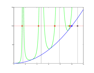
Figure 4. Graphs of $y^{2}$ (blue line) and $y^{2}\sec^{2}(y)$ (green line). Given a height $L^{2}$ (red line) the red X’s mark the roots of $y^{2}\sec^{2}(y)=L^{2}$ at which $\tan(y)>0$, the blue * marks the root of $y^{2}=L^{2}$ and the black X marks $y=(2p-1)\pi/2$ for $p$ equal to the number of red roots. The last red root is in the interval $((2p-3)\pi/2,(2p-1)\pi/2)$ if and only if $(p-1)\pi<L\leq p\pi$, i.e. $p-1<L/\pi\leq p$ and $p=\lceil L/\pi\rceil$.

Let $p=J_{s}$ be the number of roots of this last equation, let $\{y_{s,j}(h)\}_{j=1}^{p}$ be the roots of this equation, and let $L^{2}=k^{2}\overline{n}-h^{2}k^{2}n_{cl}^{2}$, then $y_{s,p}(h)\in(p\pi-3\pi/2,p\pi-\pi/2)$ if and only if $(p-1)\pi<L\leq p\pi$,so that $(p-1)<L/\pi\leq p$ and $p=\lceil L/p\rceil$.

In summary, this equation admits exactly $\Big{\lceil}\frac{1}{\pi}\sqrt{k^{2}\overline{n}^{2}-h^{2}k^{2}n^{2}_{cl}}\Big{\rceil}$ roots (see Figure 4), and since $t\mapsto\lceil t\rceil$ is piece-wise constant and left continuous, for $h\sim 0$ we get $J_{s}=\Big{\lceil}\frac{1}{\pi}k\overline{n}\Big{\rceil}$. For the roots $\{y_{s,j}(h)\}_{j=1}^{J_{s}}$ of

$$y^{2}\sec^{2}(y)=k^{2}\overline{n}^{2}-h^{2}k^{2}n_{cl}^{2} \wedge \quad\tan(y)>0,y>0.$$

letting $y_{a,s}=y_{a,s}(0)$ we observe that $y_{s,j}(h)=y_{s,j}+O(h^{2})$ for $h\sim 0$, also

(3) $$|\cos(y_{s,j})|<1\textnormal{ and }0<y_{s,j}<k\overline{n},\forall j=1,...,J_{s}.$$

For the roots of the original equation this means that there are $J_{s}$ roots $\lambda_{s,j}$ and they satisfy $\lambda_{s,j}=y^{2}_{s,j}(h)/h^{2}=y^{2}_{s,j}/h^{2}+O(1)$.

For the asymmetric guided modes the situation is similar. The equation for the roots is,

$$\sqrt{d^{2}-\lambda}+\sqrt{\lambda}\cot(h\sqrt{\lambda})=0 \wedge \quad 0<\lambda\leq d^{2},$$

$$\Leftrightarrow\quad d^{2}-\lambda=\lambda\cot^{2}(h\sqrt{\lambda}) \wedge \quad\cot(h\sqrt{\lambda})<0,$$

$$\Leftrightarrow\quad h^{2}d^{2}-h^{2}\lambda=h^{2}\lambda\cot^{2}(\sqrt{h^{2}\lambda}) \wedge \quad\cot(\sqrt{h^{2}\lambda})<0,$$

again, for $y^{2}=h^{2}\lambda$,

$$\Leftrightarrow\quad k^{2}\overline{n}^{2}-h^{2}k^{2}n_{cl}^{2}=y^{2}(1+\cot^{2}(y))=\left(\frac{y}{\sin(y)}\right)^{2}\quad \wedge \quad\cot(y)<0,y>0.$$

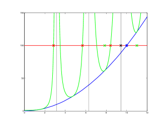
Figure 5. Graphs of $y^{2}$ (blue line) and $(y/\sin(y))^{2}$ (green line). Given a hight $L^{2}$ (red line) the red X’s mark the roots of $(y/\sin(y))^{2}=L^{2}$ at which $\cot(y)<0$, the blue * marks the root of $y^{2}=L^{2}$ and the black X marks $y=p\pi$ for $p$ equal to the number of red roots. The last red root is in the interval $((p-1)\pi,p\pi)$ if and only if $(p-1/2)\pi<L\leq(p+1/2)\pi$, i.e. $p-1<L/\pi-1/2\leq p$ and $p=\lceil L/\pi-1/2\rceil$.

Hence there are exactly $\Big{\lceil}\frac{1}{\pi}\sqrt{k^{2}\overline{n}^{2}-h^{2}k^{2}n^{2}_{cl}}-1/2\Big{\rceil}$ roots (see Figure 5), which for $h\sim 0$ is exactly $J_{a}=\Big{\lceil}\frac{1}{\pi}k\overline{n}-1/2\Big{\rceil}$. Let $\{y_{a,j}(h)\}_{j=1}^{J_{a}}$ be the roots of

$$\left(\frac{y}{\sin(y)}\right)^{2}=k^{2}\overline{n}^{2}-h^{2}k^{2}n_{cl}^{2} \wedge \quad\cot(y)<0,y>0.$$

letting $y_{a,j}=y_{a,j}(0)$, then $y_{a,j}(h)=y_{a,j}+O(h^{2})$ for $h\sim 0$ and $0<y_{s,j}<k\overline{n}$, also

(4) $$|\sin(y_{a,j})|<1\textnormal{ and }0<y_{a,j}<k\overline{n},\forall j=1,...,J_{a}.$$

For the roots of the original equation this means that there are $J_{a}$ roots $\lambda_{a,j}$ and they satisfy $\lambda_{a,s}=y^{2}_{a,s}(h)/h^{2}=y^{2}_{a,s}/h^{2}+O(1)$.

Let $c>0$ be fixed ($c>h)$ and $x\geq c$, the behavior of the $\lambda_{m,j}$’s allows us to obtain the following estimates: since $\sqrt{d^{2}-\lambda_{m,j}}=\frac{1}{h}(1+O(h^{2}))\sqrt{k^{2}\overline{n}^{2}-y^{2}_{m,j}}$ for $h\sim 0$, then

$$v_{s}(x,\lambda_{s,j}) =\cos(h\sqrt{\lambda_{s,j}})e^{-\sqrt{d^{2}-\lambda_{s,j}}(x-h)},$$

$$=(1+O(h^{2}))\cos(y_{s,j})e^{-\frac{x}{h}(1+O(h))\sqrt{k^{2}\overline{n}^{2}-y^{2}_{j,s}}}.$$

$$v_{a}(x,\lambda_{a,j}) =\sin(h\sqrt{\lambda_{a,j}})e^{-\sqrt{d^{2}-\lambda_{a,j}}(x-h)},$$

$$=(1+O(h^{2}))\sin(y_{a,j})e^{-\frac{x}{h}(1+O(h))\sqrt{k^{2}\overline{n}^{2}-y^{2}_{a,s}}}.$$

Also $k\beta_{m,j}=\sqrt{k^{2}n_{0}^{2}-\lambda_{m,j}}=\frac{1}{h}(1+O(h^{2}))\sqrt{k^{2}\overline{n}^{2}-y^{2}_{m,j}}$ and

$$\frac{e^{ik\beta_{m,j}|z-z_{0}|}}{2ik\beta_{m,j}}\frac{\sqrt{d^{2}-\lambda_{m,j}}}{1+h\sqrt{d^{2}-\lambda_{m,j}}} =\frac{e^{\frac{i}{h}(1+O(h^{2}))\sqrt{k^{2}\overline{n}^{2}-y^{2}_{m,j}}|z-z_{0}|}}{2i}\frac{1+O(h^{2})}{1+\sqrt{k^{2}\overline{n}^{2}-y^{2}_{m,j}}}.$$

Putting together all these calculations in the expression of the guided component of the Green’s function concludes the proof. ∎

3.2. Asymptotic analysis of the continuous components in the non-radiating cases.

For the asymptotic analysis of the continuous components of the Green’s function, we need to study the symmetric and asymmetric components in the radiating and non-radiating frequencies. Let us first analyze the symmetric part in the case that $\sin(k\overline{n})\neq 0$.

Lemma 11.

Let $c>0$ be fixed, let $x,x_{0}\geq c$, $|z-z_{0}|\geq c$ and assume that $\sin(k\overline{n})\neq 0$, then

$$G_{s,c}(x,z;x_{0},z_{0})= \frac{1}{2\pi}\int_{0}^{\infty}\sin(k\tau x)\sin(k\tau x_{0})\frac{e^{ik\sqrt{n^{2}_{cl}-\tau^{2}}|z-z_{0}|}}{i\sqrt{n^{2}_{cl}-\tau^{2}}}d\tau$$

$$-h\frac{1}{2\pi}\int_{0}^{\infty}\left(\frac{\cot(k\overline{n})}{k\overline{n}}+1\right)\sin(k\tau(x+x_{0}))\cdot$$

$$\cdot\frac{e^{ik\sqrt{n^{2}_{cl}-\tau^{2}}|z-z_{0}|}}{i\sqrt{n^{2}_{cl}-\tau^{2}}}k\tau d\tau+O(h^{2-4\epsilon}).$$

Proof.

The continuous symmetric part has the expression,

$$G_{s,c}(x,z;x_{0},z_{0})= \frac{1}{2\pi}\int_{d^{2}}^{\infty}v_{s}(x,\lambda)v_{s}(x_{0},\lambda)\frac{e^{ik\beta|z-z_{0}|}}{2ik\beta}\frac{\sqrt{\lambda-d^{2}}}{(\lambda-d^{2})+d^{2}\sin^{2}(h\sqrt{\lambda})}d\lambda$$

and let us consider the change of variable $k^{2}\tau^{2}=\lambda-d^{2}=\lambda-k^{2}n_{0}^{2}+k^{2}n^{2}_{cl}=k^{2}n_{cl}^{2}-k^{2}\beta^{2}$ then (multiplying and dividing by $h^{2}$),

$$G_{s,c}(x,z;x_{0},z_{0})= \frac{1}{2\pi}\int_{0}^{\infty}hv_{s}(x,k^{2}\tau^{2}+d^{2})hv_{s}(x_{0},k^{2}\tau^{2}+d^{2})\cdot$$

$$\cdot\frac{e^{ik\sqrt{n^{2}_{cl}-\tau^{2}}|z-z_{0}|}}{2ik\sqrt{n^{2}_{cl}-\tau^{2}}}\frac{k\tau}{h^{2}k^{2}\tau^{2}+h^{2}d^{2}\sin^{2}(h\sqrt{k^{2}\tau^{2}+d^{2}})}2k^{2}\tau d\tau$$

and for $x\geq c>h$, since $Q=\sqrt{\lambda-d^{2}}=k\tau$, we have that

$$hv_{s}(x,k^{2}\tau^{2}+d^{2}) =h\cos(h\sqrt{k^{2}\tau^{2}+d^{2}})\cos(k\tau(x-h))$$

$$-h\sqrt{k^{2}\tau^{2}+d^{2}}\sin(h\sqrt{k^{2}\tau^{2}+d^{2}})\frac{\sin(k\tau(x-h))}{k\tau}.$$

Since $h^{2}d^{2}=k^{2}\overline{n}^{2}+O(h^{2})$, for $\tau\in[0,h^{-\epsilon}]$ and $x\geq c>h$, we have

$$hv_{s}(x,k^{2}\tau^{2}+d^{2}) =-k\overline{n}\sin(k\overline{n})\frac{\sin(k\tau x)}{k\tau}$$

$$+h\big{(}\cos(k\overline{n})+k\overline{n}\sin(k\overline{n})\big{)}\cos(k\tau x)+O(h^{2-2\epsilon}),$$

while, since $\sin(k\overline{n})\neq 0$,

$$\frac{2k^{3}\tau^{2}}{h^{2}k^{2}\tau^{2}+h^{2}d^{2}\sin^{2}(h\sqrt{k^{2}\tau^{2}+d^{2}})}=\frac{2k^{3}\tau^{2}}{k^{2}\overline{n}^{2}\sin^{2}(k\overline{n})}+O(h^{2-4\epsilon}).$$

The previous estimates provide us an asymptotic formula of the integral when restricted to integration over $\tau\in[0,h^{-\epsilon}]$. On the other hand, since $|z-z_{0}|\geq c>0$, the term $e^{ik\sqrt{n_{cl}-\tau}}$ decays fast enough over $\tau\in[h^{-\epsilon},\infty)$, and the tail of the integral integrates to order $o(h^{2})$ for $h\sim 0$.

When using the previous calculations in the expression of $G_{s,c}$ we conclude the Lemma. ∎

Corollary 12.

Let $c>0$ be fixed, let $x_{0}\geq c$, $x<-c$, $|z-z_{0}|\geq c$ and assume that $\sin(k\overline{n})\neq 0$, then

$$G_{s,c}(x,z;x_{0},z_{0})= -\frac{1}{2\pi}\int_{0}^{\infty}\sin(k\tau x)\sin(k\tau x_{0})\frac{e^{ik\sqrt{n^{2}_{cl}-\tau^{2}}|z-z_{0}|}}{i\sqrt{n^{2}_{cl}-\tau^{2}}}d\tau+O(h),$$

i.e. the opposite sign as when $x>c$.

Proof.

It follows from the calculations made for Lemma 11 and the observation that for $x<-h$

$$hv_{s}(x,k^{2}\tau^{2}+d^{2})= h\cos(h\sqrt{k^{2}\tau^{2}+d^{2}})\cos(k\tau(x+h))$$

$$+h\sqrt{k^{2}\tau^{2}+d^{2}}\sin(h\sqrt{k^{2}\tau^{2}+d^{2}})\frac{\sin(k\tau(x+h))}{k\tau}$$

$$= k\overline{n}\sin(k\overline{n})\frac{\sin(k\tau x)}{k\tau}+O(h).$$

∎

For the asymmetric continuous part of the Green’s function we can do something similar when $\cos(k\overline{n})\neq 0$.

Lemma 13.

Let $c>0$ be fixed, let $x,x_{0}\geq c,|z-z_{0}|\geq c$ and assume that $\cos(k\overline{n})\neq 0$, then

$$G_{a,c}(x,z;x_{0},z_{0})= \frac{1}{2\pi}\int_{0}^{\infty}\sin(k\tau x)\sin(k\tau x_{0})\frac{e^{ik\sqrt{n^{2}_{cl}-\tau^{2}}|z-z_{0}|}}{i\sqrt{n^{2}_{cl}-\tau^{2}}}d\tau$$

$$+h\frac{1}{2\pi}\int_{0}^{\infty}\left(\frac{\tan(k\overline{n})}{k\overline{n}}-1\right)\sin(k\tau(x+x_{0}))\cdot$$

$$\cdot\frac{e^{ik\sqrt{n^{2}_{cl}-\tau^{2}}|z-z_{0}|}}{i\sqrt{n^{2}_{cl}-\tau^{2}}}k\tau d\tau+O(h^{2-4\epsilon}).$$

Proof.

The asymmetric continuous part of the Green’s function is,

$$G_{a,c}(x,z;x_{0},z_{0})= \frac{1}{2\pi}\int_{0}^{\infty}hv_{a}(x,k^{2}\tau^{2}+d^{2})hv_{a}(x_{0},k^{2}\tau^{2}+d^{2})\cdot$$

$$\cdot\frac{e^{ik\sqrt{n^{2}_{cl}-\tau^{2}}|z-z_{0}|}}{2ik\sqrt{n^{2}_{cl}-\tau^{2}}}\frac{2k^{3}\tau^{2}}{h^{2}k^{2}\tau^{2}+h^{2}d^{2}\cos^{2}(h\sqrt{k^{2}\tau^{2}+d^{2}})}d\tau,$$

and for $x\geq c>h$ and $\tau\in[0,h^{-\epsilon}]$, (and since $h^{2}d^{2}=k^{2}\overline{n}^{2}+O(h^{2})$)

$$hv_{a}(x,k^{2}\tau^{2}+d^{2}) =h\sin(h\sqrt{k^{2}\tau^{2}+d^{2}})\cos(k\tau(x-h))$$

$$\quad+h\sqrt{k^{2}\tau^{2}+d^{2}}\cos(h\sqrt{k^{2}\tau^{2}+d^{2}})\frac{\sin(k\tau(x-h))}{k\tau}$$

$$=k\overline{n}\cos(k\overline{n})\frac{\sin(k\tau x)}{k\tau}$$

$$\quad+h\big{(}\sin(k\overline{n})-k\overline{n}\cos(k\overline{n})\big{)}\cos(k\tau x)+O(h^{2-2\epsilon}),$$

while, if $\cos(k\overline{n})\neq 0$,

$$\frac{2k^{3}\tau^{2}}{h^{2}k^{2}\tau^{2}+h^{2}d^{2}\cos^{2}(h\sqrt{k^{2}\tau^{2}+d^{2}})}=\frac{2k^{3}\tau^{2}}{k^{2}\overline{n}^{2}\cos^{2}(k\overline{n})},+O(h^{2-4\epsilon}).$$

For the tail of the integral, over $\tau\in[h^{-\epsilon},\infty)$, because $|z-z_{0}|\geq c>0$ the exponential decay of the integrand ensures that the contribution of tail of the integral is small enough.

Using these calculations in the expression of $G_{a,c}$ conclude the proof. ∎

Corollary 14.

Let $c>0$ be fixed, let $x_{0}\geq c,x<-c,|z-z_{0}|\geq c$ and assume that $\cos(k\overline{n})\neq 0$, then

$$G_{a,c}(x,z;x_{0},z_{0})= \frac{1}{2\pi}\int_{0}^{\infty}\sin(k\tau x)\sin(k\tau x_{0})\frac{e^{ik\sqrt{n^{2}_{cl}-\tau^{2}}|z-z_{0}|}}{i\sqrt{n^{2}_{cl}-\tau^{2}}}d\tau+O(h),$$

i.e. the same sign as when $x>c$.

Proof.

It follows from the calculations made for Lemma 13 and the fact that

$$hv_{a}(x,k^{2}\tau^{2}+d^{2}) =-h\sin(h\sqrt{k^{2}\tau^{2}+d^{2}})\cos(k\tau(x+h))$$

$$\quad+h\sqrt{k^{2}\tau^{2}+d^{2}}\cos(h\sqrt{k^{2}\tau^{2}+d^{2}})\frac{\sin(k\tau(x+h))}{k\tau}$$

$$=k\overline{n}\cos(k\overline{n})\frac{\sin(k\tau x)}{k\tau}+O(h).$$

∎

3.3. Asymptotic analysis of the continuous component in the radiating cases.

In the case that $\sin(k\overline{n})=0$ the asymptotic analysis of the symmetric continuous component of the Green’s function need to be done in a different way, same for the asymmetric continuous component when $\cos(k\overline{n})=0$. Let us study the symmetric part first.

Lemma 15.

Fix $c>0$ and let $x,x_{0}\geq c$ and $|z-z_{0}|\geq c$. Assume that $\sin(k\overline{n})=0$, then

$$G_{s,c}(x,z;x_{0},z_{0})= \frac{1}{2\pi}\int_{0}^{\infty}\cos(k\tau x)\cos(k\tau x_{0})\frac{e^{ik\sqrt{n^{2}_{cl}-\tau^{2}}|z-z_{0}|}}{i\sqrt{n^{2}_{cl}-\tau^{2}}}d\tau$$

$$+h\frac{1}{2\pi}\int_{0}^{\infty}\frac{\tau^{2}+n_{cl}^{2}}{2\tau^{2}}\sin(k\tau(x+x_{0}))\frac{e^{ik\sqrt{n^{2}_{cl}-\tau^{2}}|z-z_{0}|}}{i\sqrt{n^{2}_{cl}-\tau^{2}}}k\tau d\tau$$

$$-h\frac{1}{2}\frac{kn_{cl}^{2}}{2}\frac{e^{ikn_{cl}|z-z_{0}|}}{2ikn_{cl}}2k+O(h^{3/2-4\epsilon}).$$

Proof.

In the analysis above for the continuous symmetric component, let us recall that after the change of variable $k^{2}\tau^{2}=\lambda-d^{2}=\lambda-k^{2}n_{0}^{2}+k^{2}n^{2}_{cl}=k^{2}n_{cl}^{2}-k^{2}\beta^{2}$ we obtained,

$$G_{s,c}(x,z;x_{0},z_{0})= \frac{1}{2\pi}\int_{0}^{\infty}v_{s}(x,k^{2}\tau^{2}+d^{2})v_{s}(x_{0},k^{2}\tau^{2}+d^{2})\cdot$$

$$\cdot\frac{e^{ik\sqrt{n^{2}_{cl}-\tau^{2}}|z-z_{0}|}}{2ik\sqrt{n^{2}_{cl}-\tau^{2}}}2k\frac{k^{2}\tau^{2}}{k^{2}\tau^{2}+d^{2}\sin^{2}(h\sqrt{k^{2}\tau^{2}+d^{2}})}d\tau,$$

where, for $x\geq c>h$,

$$v_{s}(x,k^{2}\tau^{2}+d^{2}) =\cos(h\sqrt{k^{2}\tau^{2}+d^{2}})\cos(k\tau(x-h))$$

$$-\sqrt{k^{2}\tau^{2}+d^{2}}\sin(h\sqrt{k^{2}\tau^{2}+d^{2}})\frac{\sin(k\tau(x-h))}{k\tau}.$$

Let us analyze the term $h\sqrt{k^{2}\tau^{2}+d^{2}}$ for $\tau\in[0,h^{-\epsilon}]$ and $x\geq c>h$. We have

$$h\sqrt{k^{2}\tau^{2}+d^{2}} =\sqrt{h^{2}d^{2}+k^{2}\tau^{2}}$$

$$=\sqrt{k^{2}\overline{n}^{2}+h^{2}k^{2}(\tau^{2}-n_{cl}^{2})}$$

$$=k\overline{n}\sqrt{1+h^{2}(\tau^{2}-n_{cl}^{2})/\overline{n}}$$

$$=k\overline{n}(1+\frac{h^{2}(\tau^{2}-n_{cl}^{2})}{2\overline{n}^{2}}+O(h^{4(1-\epsilon)}))$$

$$=k\overline{n}+\frac{h^{2}k(\tau^{2}-n_{cl}^{2})}{2\overline{n}}+O(h^{4(1-\epsilon)}),$$

in particular, if $\sin(k\overline{n})=0$, then $\cos(k\overline{n})=\pm 1$ and

$$\sin(h\sqrt{k^{2}\tau^{2}+d^{2}}) =\pm\frac{h^{2}k(\tau^{2}-n_{cl}^{2})}{2\overline{n}}+O(h^{4(1-\epsilon)}),$$

$$\cos(h\sqrt{k^{2}\tau^{2}+d^{2}}) =\pm 1+O(h^{4(1-\epsilon)}),\textnormal{ and }$$

$$\sin^{2}(h\sqrt{k^{2}\tau^{2}+d^{2}}) =\frac{h^{4}k^{2}(\tau^{2}-n_{cl}^{2})^{2}}{4\overline{n}^{2}}+O(h^{6(1-\epsilon)}).$$

Recall that

$$h^{2}d^{2} =k^{2}\overline{n}^{2}+O(h^{2}).$$

This, in turn, means that

$$v_{s}(x,k^{2}\tau^{2}+d^{2}) =\cos(h\sqrt{k^{2}\tau^{2}+d^{2}})\cos(k\tau(x-h))$$

$$-h(h\sqrt{k^{2}\tau^{2}+d^{2}})\frac{\sin(h\sqrt{k^{2}\tau^{2}+d^{2}})}{h^{2}}\frac{\sin(k\tau(x-h))}{k\tau}$$

$$=\pm\left(\cos(k\tau x)+h\tau k\frac{\tau^{2}+n_{cl}^{2}}{2\tau^{2}}\sin(k\tau x)\right)+O(h^{2(1-\epsilon)}).$$

On the other hand

$$\frac{k^{2}\tau^{2}}{k^{2}\tau^{2}+d^{2}\sin^{2}(h\sqrt{k^{2}\tau^{2}+d^{2}})}d\tau =d\tau-\frac{d^{2}\sin^{2}(h\sqrt{k^{2}\tau^{2}+d^{2}})}{k^{2}\tau^{2}+d^{2}\sin^{2}(h\sqrt{k^{2}\tau^{2}+d^{2}})}d\tau.$$

For the second term in the right hand side we separate the interval $[0,h^{-\epsilon}]$ into two intervals. For $\tau\in[h^{1/4},h^{-\epsilon}]$ we have

$$\frac{d^{2}\sin^{2}(h\sqrt{k^{2}\tau^{2}+d^{2}})}{k^{2}\tau^{2}+d^{2}\sin^{2}(h\sqrt{k^{2}\tau^{2}+d^{2}})}d\tau =O(h^{3/2-4\epsilon}).$$

and similarly

$$\frac{h^{2}k^{4}n_{cl}^{4}/4}{k^{2}\tau^{2}+h^{2}k^{4}n_{cl}^{4}/4}d\tau =O(h^{3/2}).$$

For $\tau\in[0,h^{1/4}]$ we use that

$$\frac{c}{a+c}=\frac{b}{a+b}(1-\frac{a}{a+c}(1-\frac{c}{b})),$$

$$0\leq\frac{k^{2}\tau^{2}}{k^{2}\tau^{2}+d^{2}\sin^{2}(h\sqrt{k^{2}\tau^{2}+d^{2}})}\leq 1,\textnormal{ and }$$

$$1-\frac{d^{2}\sin^{2}(h\sqrt{k^{2}\tau^{2}+d^{2}})}{h^{2}k^{4}n_{cl}^{4}/4}=O(h^{1/2})\textnormal{ for }\tau\in[0,\tau^{1/4}],$$

to obtain

$$\frac{d^{2}\sin^{2}(h\sqrt{k^{2}\tau^{2}+d^{2}})}{k^{2}\tau^{2}+d^{2}\sin^{2}(h\sqrt{k^{2}\tau^{2}+d^{2}})}d\tau =\frac{h^{2}k^{4}n_{cl}^{4}/4}{k^{2}\tau^{2}+h^{2}k^{4}n_{cl}^{4}/4}d\tau\cdot$$

$$\cdot\Bigg{(}1-\frac{k^{2}\tau^{2}}{k^{2}\tau^{2}+d^{2}\sin^{2}(h\sqrt{k^{2}\tau^{2}+d^{2}})}\cdot$$

$$\cdot\left(1-\frac{d^{2}\sin^{2}(h\sqrt{k^{2}\tau^{2}+d^{2}})}{h^{2}k^{4}n_{cl}^{4}/4}\right)\Bigg{)}$$

$$=\frac{h^{2}k^{4}n_{cl}^{4}/4}{k^{2}\tau^{2}+h^{2}k^{4}n_{cl}^{4}/4}d\tau(1+O(h^{1/2}))$$

$$=h\frac{kn_{cl}^{2}}{2}\left(\frac{h}{(\frac{2\tau}{kn_{cl}^{2}})^{2}+h^{2}}\frac{2d\tau}{kn_{cl}^{2}}\right)(1+O(h^{1/2})).$$

In summary, for $\tau\in[0,h^{-\epsilon}]$

$$\frac{k^{2}\tau^{2}}{k^{2}\tau^{2}+d^{2}\sin^{2}(h\sqrt{k^{2}\tau^{2}+d^{2}})}d\tau =d\tau-h\frac{kn_{cl}^{2}}{2}\left(\frac{h}{(\frac{2\tau}{kn_{cl}^{2}})^{2}+h^{2}}\frac{2d\tau}{kn_{cl}^{2}}\right)(1+O(h^{1/2}))+$$

$$+O(h^{3/2-4\epsilon})$$

and we observe that the second term in the right hand side is the Poisson kernel. Since the integrand decays exponentially fast for $\tau\in[h^{-\epsilon},\infty]$ when $|z-z_{0}|\geq c>0$ and recalling again that the Poisson Kernel satisfies

$$\int_{\mathbb{R}}f(t)\frac{h}{t^{2}+h^{2}}dt=\pi f(0)+O(h^{1/2})$$

we put together all the previous estimates to conclude the asymptotic formula. ∎

Corollary 16.

Fix $c>0$, let $x_{0}\geq c$, $x<-c$ and $|z-z_{0}|\geq c$. Assume that $\sin(k\overline{n})=0$, then

$$G_{s,c}(x,z;x_{0},z_{0})= \frac{1}{2\pi}\int_{0}^{\infty}\cos(k\tau x)\cos(k\tau x_{0})\frac{e^{ik\sqrt{n^{2}_{cl}-\tau^{2}}|z-z_{0}|}}{i\sqrt{n^{2}_{cl}-\tau^{2}}}d\tau+O(h),$$

i.e. the same sign as when $x>c$.

Proof.

It follows from the calculations in Lemma 15 and the observation that for both $x_{0}>c$ and $x<-c$

$$v_{s}(x_{0},k^{2}\tau^{2}+d^{2})= \cos(h\sqrt{k^{2}\tau^{2}+d^{2}})\cos(k\tau(x_{0}-h))$$

$$-h(h\sqrt{k^{2}\tau^{2}+d^{2}})\frac{\sin(h\sqrt{k^{2}\tau^{2}+d^{2}})}{h^{2}}\frac{\sin(k\tau(x_{0}-h))}{k\tau}$$

$$=\pm\cos(k\tau x_{0})+O(h)\quad\textnormal{ and}$$

$$v_{s}(x,k^{2}\tau^{2}+d^{2})= \cos(h\sqrt{k^{2}\tau^{2}+d^{2}})\cos(k\tau(x+h))$$

$$+h(h\sqrt{k^{2}\tau^{2}+d^{2}})\frac{\sin(h\sqrt{k^{2}\tau^{2}+d^{2}})}{h^{2}}\frac{\sin(k\tau(x+h))}{k\tau}$$

$$=\pm\cos(k\tau x)+O(h).$$

∎

For the asymmetric continuous part, when $\cos(k\overline{n})=0$, we can switch the roles of the sines and cosines in the computations above to conclude in an analogous manner the following results.

Lemma 17.

Fix $c>0$ and let $x,x_{0}\geq c$ and $|z-z_{0}|\geq c$. Assume that $\cos(k\overline{n})=0$, then

$$G_{a,c}(x,z;x_{0},z_{0})= \frac{1}{2\pi}\int_{0}^{\infty}\cos(k\tau x)\cos(k\tau x_{0})\frac{e^{ik\sqrt{n^{2}_{cl}-\tau^{2}}|z-z_{0}|}}{i\sqrt{n^{2}_{cl}-\tau^{2}}}d\tau$$

$$+h\frac{1}{2\pi}\int_{0}^{\infty}\frac{\tau^{2}+n_{cl}^{2}}{2\tau^{2}}\sin(k\tau(x+x_{0}))\frac{e^{ik\sqrt{n^{2}_{cl}-\tau^{2}}|z-z_{0}|}}{i\sqrt{n^{2}_{cl}-\tau^{2}}}k\tau d\tau$$

$$-h\frac{1}{2}\frac{kn_{cl}^{2}}{2}\frac{e^{ikn_{cl}|z-z_{0}|}}{2ikn_{cl}}2k+O(h^{3/2-4\epsilon}).$$

Corollary 18.

Fix $c>0$, let $x_{0}\geq c$, $x<-c$ and $|z-z_{0}|\geq c$. Assume that $\cos(k\overline{n})=0$, then

$$G_{a,c}(x,z;x_{0},z_{0})= -\frac{1}{2\pi}\int_{0}^{\infty}\cos(k\tau x)\cos(k\tau x_{0})\frac{e^{ik\sqrt{n^{2}_{cl}-\tau^{2}}|z-z_{0}|}}{i\sqrt{n^{2}_{cl}-\tau^{2}}}d\tau+O(h),$$

i.e. the opposite sign as when $x>c$.

Proof.

To confirm the change of sign we observe that

$$v_{a}(x_{0},k^{2}\tau^{2}+d^{2})= \sin(h\sqrt{k^{2}\tau^{2}+d^{2}})\cos(k\tau(x_{0}-h))$$

$$+h(h\sqrt{k^{2}\tau^{2}+d^{2}})\frac{\cos(h\sqrt{k^{2}\tau^{2}+d^{2}})}{h^{2}}\frac{\sin(k\tau(x_{0}-h))}{k\tau}$$

$$=\pm\cos(k\tau x_{0})+O(h),\quad\textnormal{ while}$$

$$v_{a}(x,k^{2}\tau^{2}+d^{2})= -\sin(h\sqrt{k^{2}\tau^{2}+d^{2}})\cos(k\tau(x+h))$$

$$+h(h\sqrt{k^{2}\tau^{2}+d^{2}})\frac{\cos(h\sqrt{k^{2}\tau^{2}+d^{2}})}{h^{2}}\frac{\sin(k\tau(x+h))}{k\tau}$$

$$=\mp\cos(k\tau x)+O(h).$$

∎

3.4. Helmoltz equation in the homogeneous plane.

Lemma 19.

Consider the Green’s function problem for the Helmholtz equation in the plane,

$$\Delta G_{H}+k^{2}n^{2}G_{H}=\delta(x-x_{0})\delta(z-z_{0}),\qquad(x,z)\in\mathbb{R}^{2}$$

then

$$G_{H}(x,z;x_{0},z_{0};k)= \frac{1}{2\pi}\int_{0}^{\infty}\cos(k\tau(x-x_{0}))\frac{e^{ik\sqrt{n^{2}-\tau^{2}}|z-z_{0}|}}{i\sqrt{n^{2}-\tau^{2}}}d\tau.$$

Proof.

Taking Fourier transform in $x\mapsto\omega$ variable, and denoting by $\hat{G}_{H}$ the Fourier transform of $G_{H}$ in the $x$ variable, the equation becomes

$$\partial_{z}^{2}\hat{G}_{H}+(k^{2}n^{2}-w^{2})\hat{G}_{H}=e^{-i\omega x_{0}}\delta(z-z_{0}),$$

which then implies that for each $\omega$

$$\hat{G}_{H}=e^{-i\omega x_{0}}\frac{e^{i\sqrt{k^{2}n^{2}-\omega^{2}}|z-z_{0}|}}{2i\sqrt{k^{2}n^{2}-\omega^{2}}}.$$

Taking inverse Fourier transform in $\omega$ we get

$$G_{H}= \frac{1}{2\pi}\int_{-\infty}^{\infty}e^{iwz}e^{-i\omega x_{0}}\frac{e^{i\sqrt{k^{2}n^{2}-\omega^{2}}|z-z_{0}|}}{2i\sqrt{k^{2}n^{2}-\omega^{2}}}dw$$

$$= \frac{1}{2\pi}\int_{0}^{\infty}\cos(w(x-x_{0}))\frac{e^{i\sqrt{k^{2}n^{2}-\omega^{2}}|z-z_{0}|}}{i\sqrt{k^{2}n^{2}-\omega^{2}}}dw,$$

and considering the change of variable $\omega=k\tau$ we conclude

$$G_{H}(x,z;x_{0},z_{0};k)= \frac{1}{2\pi}\int_{0}^{\infty}\cos(k\tau(x-x_{0}))\frac{e^{ik\sqrt{n^{2}-\tau^{2}}|z-z_{0}|}}{i\sqrt{n^{2}-\tau^{2}}}d\tau.$$

∎

The Green’s function $G^{H}$ also satisfies the following properties.

Lemma 20.

If $x_{1},x_{2}<0$ and $G^{H}(0,z;x_{1},z_{1})-G^{H}(0,z;,x_{2},z_{2})=0,\forall z\in[0,1]$ then $(x_{1},x_{2})=(x_{2},z_{2})$.

Proof.

Let $W(x,z):=G^{H}(x,z;x_{1},z_{1})-G^{H}(x,z;,x_{2},z_{2})$. Since $G^{H}(0,z;x_{j},z_{j})=-\frac{i}{4}H\left(kn_{cl}\sqrt{x_{j}^{2}+(z-z_{j})^{2}}\right)$, and $H$ the Hankel function is holomorphic in the complex plane cut along the negative real axis, then $z\mapsto W(0,z)$ can be extended analytically to $z\in\mathbb{C}\times i[-\epsilon,\epsilon]$ (for $\epsilon<\min\{|x_{1}|,|x_{2}|\}$). But since $W(0,z)$ vanishes for $z\in[0,1]$ then $W(0,z)=0,\forall z\in\mathbb{R}$. But we also have that $W(x,z)$ solves the homogeneous Helmholtz equation without source in $x>0$ (since $x_{1},x_{2}<0$), with standard radiation conditions, so $W(0,z)=0$ implies $W(x,z)=0$ for all $x\geq 0,z\in\mathbb{R}$. Since $W(x,z)$ solves the homogeneous Helmoltz equation in $\mathbb{R}^{2}\setminus\{(x_{1},z_{1}),(x_{2},z_{2})\}$, unique continuation then implies that $G^{H}(x,z;x_{1},z_{1})-G^{H}(x,z;,x_{2},z_{2})=W(x,z)=0$ in $\mathbb{R}^{2}\setminus\{(x_{1},z_{1}),(x_{2},z_{2})\}$, but this can only happen if $(x_{1},z_{1})=(x_{2},z_{2})$. ∎

Lemma 21.

If $S\subset\mathbb{R}^{2}$ contains two non-parallel straight segments, and $G^{H}(x,z;x_{1},z_{1})-G^{H}(x,z;,x_{2},z_{2})=0,\forall(x,z)\in S$, then $(x_{1},x_{2})=(x_{2},z_{2})$.

Proof.

Let $W(x,z):=G^{H}(x,z;x_{1},z_{1})-G^{H}(x,z;,x_{2},z_{2})$. Let $L_{1},L_{2}$ be non-parallel lines in $\mathbb{R}^{2}$ such that $S$ contains a segment of $L_{1}$ and a segment of $L_{2}$. As done in the proof of Lemma 20, this implies that $W(x,z)=0$ over $L_{1}$ and $W(x,z)=0$ over $L_{2}$. If any $(x_{j},z_{j})$ is a point in $L_{1}\cup L_{2}$, then $W(x_{j},z_{j})=0$ implies that $(x_{1},z_{1})=(x_{2},z_{2})$ (since $\lim_{(x,z)\to(x_{j},z_{j})}|G(x,z;x_{j},z_{j})|=\infty$). If none of the $(x_{j},z_{j})$ are points in $L_{1}\cup L_{2}$, then $L_{1}\cup L_{2}$ divide $\mathbb{R}^{2}$ in four regions and we can choose $\Omega\subset\mathbb{R}^{2}$ to be one of such regions such that none of the $(x_{j},z_{j})$ are in $\overline{\Omega}$ (and $\partial\Omega\subset L_{1}\cup L_{2}$). Then $W(x,z)$ solves the homogeneous Helmholtz equation in $\Omega$ without sources, with standard radiation conditions and with vanishing boundary conditions ($W(x,z)=0$ on $\partial\Omega$), hence $W(x,z)=0$ for all $(x,z)\in\Omega$. Since $W(x,z)$ solves the homogeneous Helmoltz equation in $\mathbb{R}^{2}\setminus\{(x_{1},z_{1}),(x_{2},z_{2})\}$, unique continuation then implies that $G^{H}(x,z;x_{1},z_{1})-G^{H}(x,z;,x_{2},z_{2})=W(x,z)=0$ in $\mathbb{R}^{2}\setminus\{(x_{1},z_{1}),(x_{2},z_{2})\}$, but this can only happen if $(x_{1},z_{1})=(x_{2},z_{2})$. ∎

4. Numerical identification of the waveguide parameters

In this section we illustrate the numerical implementation of the identification algorithm proposed in Section 2 for recovering the main parameters of the waveguide: location, thickness and index of refraction, We also simulate the multifrequency observations over some receptor screen, including the effect of observation errors.

4.1. General setting

In order to check the feasibility and the robustness to noise of the proposed algorithm, we consider the following setting for the geometry of the waveguide. We assume that in the original reference system $Ox^{\prime}z^{\prime}$ the waveguide is slanted in an unknown angle $\alpha$ at an unknown distance $x_{0}$ from the source. The thickness $h$ and index of refraction $n_{0}$ of the waveguide are also unknown. We assume only that the position of the screen observation points with respect to the source location are known (see Figure 6 top). In this original system the position of the source is the origin $(0,0)$. If we rotate and translate the system $Ox^{\prime}z^{\prime}$ in an angle $\alpha$ by means of the affine linear transformation:

$$\left(\begin{array}[]{c}x\cr z\end{array}\right)=\left(\begin{array}[]{c}x_{0}\cr z_{0}\end{array}\right)+\left(\begin{array}[]{cc}\cos\alpha&-\sin\alpha\cr\sin\alpha&\cos\alpha\end{array}\right)\left(\begin{array}[]{c}x^{\prime}\cr z^{\prime}\end{array}\right)=:T_{x_{0},\alpha}(x^{\prime},z^{\prime})$$

we obtain a new system $Oxz$ where the waveguide is parallel and centered to the $z-$axis (see Figure 6 bottom). We will work in this system to be consistent with the notations of the previous theoretical sections and the corresponding asymptotic formulas, but recall that the angle $\alpha$ unknown and it is part of the inverse problem.

Figure 6. Geometry. Top: position of the point source, waveguide and screen. Bottom, same configuration after rotation. The angle of rotation $\alpha$, the distance from the point source to the waveguide $x_{0}$ (dashed line), the thickness $h$ and index of refraction $n_{0}$ of the waveguide are unknown. Multifrequency measurements of the Green function $G$ are available on the screen $S$.

In this way, the point source is located now at $(x_{0},z_{0})$ in the $Oxz$ system and we assume without loss of generality that $z_{0}=0$ is known (but not the angle of rotation $\alpha$), the origin is located at the nearest point of the axis of the waveguide to the source (see Figure 6 bottom) and $x_{0}$ is the unknown distance between the source and the (center axis) waveguide. The waveguide is given by ${\mathcal{W}}=\{(x,z)\,,\,|x|<h\}$ with longitudinal axis at $x=0$. The oblique screen receptor in $Oxz$ is described by $S=\{(x,z)\,|\,x=a_{1}(z-z_{m})+b_{1},\ z_{1}<z<z_{m},\ x=a_{2}(z-z_{m})+b_{2},\ z_{m}<z<z_{2}\}$ where $z_{m}=(z_{1}+z_{2})/2$, a piecewise linear segment (see Figure 6). For this, we select $a_{1}=0.1$, $b_{1}=0.1$, $a_{2}=-0.4$, $b_{2}=0.1$, $z_{1}=2$, $z_{2}=7$, $\alpha=\pi/20$, $x_{0}=1$ and we choose the indexes of refraction in a high contrast regime with the values $n_{0}=300$ for the waveguide and $n_{cl}=1$ for the surrounding cladding media. For the thickness of the waveguide we take $h=0.01$ so $\overline{n}=n_{0}\,h=3.0$ as defined in Section 2.

For each wavenumber $k$, the measurements over the receptor are simulated using a numerical approximation of the Green’s function introduced in Section 2. The continuous part of this Green’s function is computed using an adapted numerical integration that uses a finer mesh near the singularities of the involved integrals. Even if in most of the considered cases the guided part of the Green’s function is small compared with the continuous part (see Section 2), we compute it in order to verify their theoretical number and smallness. Finally, we add to the observations a uniform error which is proportional to some percentage of the amplitude of the real and imaginary part of the solution at each point of the receptor.

The identification problem consists in finding the location (angle $\alpha$ and distance $x_{0}$), thickness $h$ and index of refraction $n_{0}$ of the waveguide from the previous simulated multifrequency observations on the receptor screen in a frequency range $k\in[k_{min},k_{max}]$ with $k_{min}=0.2$ and $k_{max}=2.0$ where we suppose that there exists a first radiating resonance at a certain unknown wavenumber $k^{*}_{1}$.

4.2. First step: searching for the first radiating resonance

Starting from the initial guess values $\alpha=0.1$, $x_{0}=0.5$, $n_{0}=100$ and $h=0.05$, we search for the wavenumber $k^{*}_{1}$ of the first radiating resonance by probing the media in a successively smaller and finer range of frequencies.

More precisely, we implement the search as it is shown in Figure 7. We compute the $L^{2}$-norm of the measurements on the reception screen. We start the searching process with a frequency step of $\Delta k=k_{max}/100$ in the whole frequency range $[k_{min},k_{max}]$ and we find a first approximation $k^{*(1)}_{1}$ of $k^{*}_{1}$ by searching the first point of local maximum convexity of the curve. Then we repeat the process twice with smaller frequency steps and smaller frequency ranges by searching this time the point of maximum amplitude of the curve in order to estimate the value of $k^{*}_{1}$ with a finer precision. In the second step we use $\Delta k=k^{*(1)}_{1}/100$ and frequency range $[0.9k^{*(1)}_{1},1.1k^{*(1)}_{1}]$ obtaining a new approximation $k^{*(2)}_{1}$ and finally we set $\Delta k=k^{*(2)}_{1}/1000$ and frequency range $[0.99k^{*(2)}_{1},1.01k^{*(2)}_{1}]$ to obtain the final approximation of $k^{*}_{1}$ shown in Table 1.

This method allows us to recover $k^{*}_{1}$ with good accuracy independently of the observation error level as this can be noticed in Table 1. Since $k^{*}_{1}$ is the first zero of $\sin(2k^{*}_{1}\overline{n})=0$ this also allow us to recover

$$\overline{n}=n_{0}\,h=\frac{\pi}{2k^{*}_{1}}$$

with high precision independently of the observation noise level. This completes the first step of the identification algorithm.

Figure 7. First step of the algorithm. Successive approximations of the first radiating resonance $k^{*}_{1}$ (dashed vertical line) estimated from the energy of the measurements on the receptor screen ($5\%$ noise). The first radiating resonance is approximated with increasing detail among 91 (left), 21 (center) and 17 (right) frequencies.

4.3. Second step: estimation of the location of the waveguide

In a second step, we fix a relatively non-radiative value for the frequency, for example $k=k_{0}=5.1\,k^{*}_{1}$ where $k^{*}_{1}$ is the first radiating frequency estimated in the first step. Then we find the values of $\widehat{\alpha}$ and $\widehat{x}_{0}$ that minimize the $L^{2}$-gap between the measurements of the Green function on the screen $G(k_{0})|_{S}$ at the same frequency in the original translated and rotated system (so they depend on $\alpha$ and $x_{0}$) and the first order term of the non-reflective asymptotic formula of Theorem 1:

$$G_{0}^{\textnormal{NR}}(x_{0},k_{0};x,z)=\frac{1}{\pi}\int_{0}^{\infty}\sin(k_{0}\tau x)\sin(k_{0}\tau x_{0})\frac{e^{ik\sqrt{n^{2}_{cl}-\tau^{2}}|z|}}{i\sqrt{n^{2}_{cl}-\tau^{2}}}d\tau$$

evaluated on the observation screen $S$ (see Figure 8).

$$\widehat{x}_{0},\widehat{\alpha}=\arg\min|G_{0}^{\textnormal{NR}}(x_{0},k_{0};.)|_{S}-G(k_{0})|_{S}\circ T_{-\alpha,x_{0},0}|^{2}$$

We use a standard quasi-Newton BFGS minimization method and this produces the values of the $\widehat{x}_{0}$ and $\widehat{\alpha}$ columns in Table 1. The success of this minimization step is crucial since the parameters of the next step are very sensitive to the location of the waveguide. This second step is also the more time demanding step of the algorithm.

Figure 8. Second step of the algorithm. Estimation of the rotation and position of the waveguide by minimizing the fit between the asymptotic formula (that only depends of the product $\overline{n}=n_{0}\,h$) for a non-radiating frequency $k_{0}=5.1\,k^{*}_{1}$ with the noisy observations ($5\%$ noise) on the screen $S$.

4.4. Third step: estimation of the thickness and index of refraction of the waveguide

In the last step, in order to estimate the thickness $h$, we use again the asymptotic formula of the non-reflective case Theorem 1. We can choose the same of the previous section or another value. We observed that a larger value seems better, maybe since for larger frequencies there are more oscillations in the screen, so we choose a non-reflective value of $k=5.1\,k^{*}_{1}$. From the estimated values of $\widehat{\alpha}$, $\widehat{x}_{0}$ and $\overline{n}$ of the previous steps, we compute the term $G_{1}^{NR}$ that accompanies $h$ in the asymptotic formula:

$$G_{1}^{\textnormal{NR}}(k;x,z)\!=\!\frac{1}{2\pi}\!\!\int_{0}^{\infty}\!\!\!\left(\frac{\tan(k\overline{n})-\cot(k\overline{n})}{k\overline{n}}\!-\!2\!\right)\sin(k\tau(x+\widehat{x}_{0}))\frac{e^{ik\sqrt{n^{2}_{cl}-\tau^{2}}|z|}}{i\sqrt{n^{2}_{cl}-\tau^{2}}}k\tau d\tau$$

Then we estimate $h$ as the mean of the real part of the difference between the observations and the first order term of the asymptotic formula, divided by $u_{2}$:

$$\widehat{h}=\left\langle\frac{|G_{0}^{\textnormal{NR}}(\widehat{x}_{0},k;\cdot)|_{S}-G(k)|_{S}\circ T_{-\widehat{\alpha},\widehat{x}_{0},0}|}{|G_{1}^{\textnormal{NR}}(\widehat{x}_{0},k;\cdot)|_{S}}\right\rangle.$$

This is valid for every observation point in $\mathcal{O}$ so we average the values in order to cancel as much as possible noise (see Figure 9) and by avoiding too small values of $|G_{1}^{NR}|$. This could also be improved by averaging repeated measurements (but we did it for a single one).

Finally we estimate the index of refraction by

$$\widehat{n}_{0}=\overline{n}/\widehat{h}.$$

The numerical results of this final part of the algorithm are presented in the two columns labeled $\widehat{h}$ and $\widehat{n}_{0}$ in Table 1.

Figure 9. Third step of the algorithm. Estimation of the thickness of the waveguide by averaging the correction term factor of the asymptotic formula (that does not depends on $h$ nor $n_{0}$) for a fixed non-radiating frequency $5.1\,k^{*}_{1}$ with noisy observations ($5\%$ noise).

	first step		second step		third step
parameter	$k^{*}_{1}$	$\overline{n}=n_{0}\,h$	$\widehat{x}_{0}$	$\widehat{\alpha}$	$\widehat{h}$	$\widehat{n}_{0}$
exact value	0.5236	3.000	1.000	0.1571	0.0100	300.0
error level
3%	0.5238	2.999	0.9945	0.1614	0.0133	225.5
(rel. error)	(0.04%)	(0.03%)	(0.55%)	(2.7%)	(33%)	(24%)
5%	0.5238	2.999	0.9995	0.1596	0.01429	209.9
(rel. error)	(0.04%)	(0.03%)	(1.1%)	(1.6%)	(43%)	(30%)
8%	0.5238	2.999	0.9889	0.1576	0.0202	148.3
(rel. error)	(0.04%)	(0.03%)	(1.1%)	(0.3%)	(102%)	(51%)

Table 1. Exact and estimated waveguide parameters: location $x_{0}$, inclination $\alpha$, thickness $h$ and index of refraction $n_{0}$, for different measurement error levels obtained using the three-step algorithm proposed in this section.

References

- [1] H. Ammari, F. Triki. Resonances for microstrip transmission lines. SIAM J. Appl. Math., 64(2), 601–636, 2004.
- [2] E. Bonnetier, F. Triki: Asymptotic of the Green function for the diffraction by a perfectly conducting plane perturbed by a sub-wavelength rectangular cavity. Mathematical Methods in the Applied Sciences 33(6), 772–798, 2009.
- [3] J.-P. Carini, J.T. Londergan, K. Mullen, D.P. Murdock, Bound states and resonances in waveguides and quantum wires Physical Review B, 46(23), 15538–541, 1992.
- [4] G. Ciraolo: A radiation condition for the 2-D Helmholtz equation in stratified media. Communications in Partial Differential Equations, 34(12), 1592–1606, 2009.
- [5] G. Ciraolo, R. Magnanini: A radiation condition for uniqueness in a wave propagation problem for 2d open waveguide. Math. Meth. Appl. Sci. 32, 1183–1206, 2009.
- [6] J. Fey, W.-M. Robertson: Compact acoustic bandgap material based on a subwavelength collection of detuned Helmholtz resonators. Journal of Applied Physics 109, 114903 (5 pag.), 2011.
- [7] C. Jerez-Hanckes, J.-C. Nédélec: Asymptotics for Helmholtz and Maxwell Solutions in 3-D Open Waveguides. Communications in Computacional Physics, 11(2), 629–646, 2012.
- [8] R. Magnanini, F. Santosa: Wave propagation in a 2d optical waveguide. SIAM Journal on Applied Mathematics, 61(4), 1237–1252, 2000.
- [9] P. Kuchment, The Mathematics of Photonic Crystals, in Mathematical Modeling in Optical Science, Frontiers in Applied Mathematics, SIAM, Ed. G. Bao, L. Cowsar, W. Masters, pp. 207–272, https://doi.org/10.1137/1.9780898717594.ch7, 2001.
- [10] F. Rellich, Über das asymptotische Verhalten del Lösungen von in unendlichen Gebieten, Jber. Deutsch. Math. Verein., (53) (1943), pp. 57 - 65.
- [11] G. N. Watson, A treatise on the theory of Bessel functions, Cambridge Mathematical Library, Cambridge University Press, Cambridge, 1995. Reprint of the second (1944) edition. MR1349110.
- [12] C. Wilcox, Spectral analysis of the Pekeris operator in the theory of acoustic wave propagation in shallow water, Arch. Rational Mech. Anal., 60, no. 3, pp. 259–300, 1975.