Extracting the Multiscale Causal Backbone of Brain Dynamics

Abstract

The bulk of the research effort on brain connectivity revolves around statistical associations among brain regions, which do not directly relate to the causal mechanisms governing brain dynamics. Here we propose the multiscale causal backbone (MCB) of brain dynamics shared by a set of individuals across multiple temporal scales, and devise a principled methodology to extract it.

Our approach leverages recent advances in multiscale causal structure learning and optimizes the trade-off between the model fitting and its complexity. Empirical assessment on synthetic data shows the superiority of our methodology over a baseline based on canonical functional connectivity networks. When applied to resting-state fMRI data, we find sparse MCBs for both the left and right brain hemispheres. Thanks to its multiscale nature, our approach shows that at low-frequency bands, causal dynamics are driven by brain regions associated with high-level cognitive functions; at higher frequencies instead, nodes related to sensory processing play a crucial role. Finally, our analysis of individual multiscale causal structures confirms the existence of a causal fingerprint of brain connectivity, thus supporting from a causal perspective the existing extensive research in brain connectivity fingerprinting.

Code https://github.com/OfficiallyDAC/cb.git

Keywords Causal structure learning  $\cdot$ Multiscale causal backbone  $\cdot$ Brain connectivity  $\cdot$ fMRI data

1 Introduction

The study of brain connectivity is a fundamental pursuit in neuroscience that has a rich history spanning decades (Felleman and Van Essen, 1991; Biswal et al., 1995). The development of magnetic resonance imaging (MRI) paved the way to connectomics (Sporns et al., 2005; Bullmore and Sporns, 2009), i.e., the study of the brain as a network, where nodes represent brain regions of interest (ROIs), and arcs among ROIs are defined either by observing anatomic fiber density (structural connectome), or by exploiting the link between neural activity and blood flow and oxygenation to associate a time series to each ROI and then creating a link between two ROIs that exhibit co-activation, i.e., strong correlation in their time series (functional connectome) (Fox et al., 2005).

Typical measures of functional connectivity between ROIs can be distinguished between undirected measures, which capture statistical dependence without specifying direction, and directed measures, which explore statistical causation by specifying the direction of the dependencies (Wiener, 1956; Granger, 1969). Directed connectivity measures often rely on the assumption that the cause precedes the effect, and thus focus on estimating lagged dependencies. Examples of bivariate measures include Granger causality (Granger, 1969) and transfer entropy (Schreiber, 2000). Extensions to the multivariate case include conditional Granger causality (Ding et al., 2006), partial Granger causality (Guo et al., 2008), directed transfer function (DTF, Kaminski and Blinowska, 1991), and partial directed coherence (PDC, Baccalá and Sameshima, 2001)(see  Blinowska (2011); Bastos and Schoffelen (2016) for comprehensive reviews). Directed functional connectivity measures cannot be considered causal in the strict sense, because they do not describe the underlying causal mechanisms of the observed time series.

One step closer to causal modeling is effective connectivity (Harrison et al., 2003), which studies directional and causal relationships between ROIs to understand how information flows within the brain. Effective connectivity is considered a first-order data feature: a cause of the observed functional connectivity (Razi and Friston, 2016). The reference model for effective connectivity is the dynamic causal model (DCM) by Friston et al. (2003). DCM is essentially a state-space model where the behavior and coupling of $K$ hidden neuronal states determine the variation of $K$ observed signals. However, DCM is not a causal structure learning method, but rather a model for testing specific causal hypotheses. Conversely, our work aims to infer causal relationships in a purely data-driven manner.

Specifically, given a group of individuals, where each individual is described by fMRI data (i.e., a set of time series corresponding to different ROIs, where the ROIs are the same across the individuals), we tackle the learning problem of discovering the multiscale causal backbone (MCB), the largest causal network shared by individuals that still preserves personal idiosyncrasies. Studying the brain connectivity of groups is crucial for several tasks, such as detecting diseases and disorders, designing effective therapeutic interventions, and mapping brain networks (Craddock et al., 2012; Bassett and Sporns, 2017). Conscious that brain functions vary over different time scales (Jacobs et al., 2007; Ide et al., 2017), we approach the discovery of brain causal mechanisms from a multiscale perspective. A time scale refers here to one of the resolutions at which a given signal (ROI time series in our case) is analyzed. The coarsest time scales correspond to the low-frequency components of the signal, whereas the finest to the high-frequency ones. For instance, one might be interested in coarsest time scales to examine neuronal oscillations during sleep. Conversely, one might be interested in the finest time scales to understand how neuronal populations fire in response to a specific stimulus.

We develop our method by leveraging recent advances in multiscale causal structure learning (MS-CASTLE, D’Acunto et al., 2023) to retrieve individual multiscale DAGs, i.e., a multi-layer causal graph where the brain ROIs correspond to graph nodes, and time scales to graph layers. MS-CASTLE falls under functional causal structure learning methods, expressing a node’s value as a function of parent nodes. It is a gradient-based causal discovery method, that builds upon the continuous approximation of the acyclicity property of a graph (Zheng et al., 2018). Given the learned individual multiscale DAGs, we adopt the minimum description length (MDL) principle, to detect the MCB which optimizes the trade-off between the model fitting (i.e., the likelihood of observing the data given the MCB and individual idiosyncrasies) and its complexity (i.e., the number of arcs in the multiscale causal graph consisting of the MCB and the individual idiosyncrasies).

Contributions and roadmap. We formally define the learning problem of discovering the MCB from a sample of individual fMRI recordings in resting state. We devise a methodology to solve this learning task that first uses MS-CASTLE (D’Acunto et al., 2023) to learn individual multiscale DAGs (Section 3), and then runs a score-based search procedure on top of the learned individual multiscale DAGs (Section 4). The proposed score-based search procedure is related to score-based causal structure learning methods (Heckerman et al., 1995; Chickering, 2002; Gu and Zhou, 2020). The score function we optimize however represents a generalization to the multi-subject, multiscale setting of the widely used scores for learning Gaussian Bayesian networks, e.g., the BIC score (Schwarz, 1978). Our methodology differs from multi-domain causal structure learning methods (Ghassami et al., 2018; Zeng et al., 2021; Perry et al., 2022), which instead typically learn a single causal structure from multi-domain data. Indeed, the weights of the arcs composing the MCB learned by our method vary over the subjects. In this way, we are able to both the causal structure shared across subjecs, and to preserver the idiosyncratic causal structure of each individual. Our empirical assessment on synthetic data (Section 5) shows the superiority of our method over baseline based on functional connectivity networks in the same learning task.

As an application (Section 6), we study using the proposed methodology a dataset of resting-state functional magnetic resonance imaging (rs-fMRI), constituted by $100$ healthy subjects, publicly available as part of the Human Connectome Project (HCP, Smith et al., 2013). We find that MCBs can be detected for both the left and right hemispheres, and that they are sparse. Our method also allows us to discover the ROIs driving the brain activity at different frequency bands. In particular, we find two sets of ROIs that play different roles depending on the considered frequency band. The first set of nodes, obtained for lower frequencies, is associated with high-level cognitive functions, such as self-awareness and introspection, while the second set, obtained for higher frequencies, includes nodes that are key drivers in sensory processing.

Additionally, we compare the learned MCBs with the single-scale causal backbones (SCBs). Despite the agreement of single-scale and multiscale analyses on the identification of the key drivers within the system at hand, the SCBs result in an aggregated version of the MCBs. This aggregation impairs the capability to localize (in the frequency domain) changes in the causal structure, and to distinguish that higher-level cognitive functions prevail at lower frequencies, i.e., below $0.1$ Hz, as also supported by Biswal et al. (1995); Fox et al. (2005); Van Dijk et al. (2010).

Finally, we investigate the possibility to perform causal fingerprinting, i.e., to use the variability of individual multiscale DAGs to effectively classify individuals in large-scale studies. We show that that causal fingerprinting is indeed possible at various hard-thresholding levels, and that it outperforms the canonical fingerprinting based on functional connectivity alone.

2 Preliminaries

Here we provide the notation and background information needed to formally define the problem we tackle in this paper.

Notation. The range of integers from $1$ to $Y$ is denoted by $[Y]$. Scalars are lowercase, $y$, vectors are lowercase bold, $\mathbf{y}$, and matrices are uppercase bold, $\mathbf{Y}$. Given $\mathbf{y}\in^{Y}$, the diagonal matrix of size $Y$ by $Y$ having $\mathbf{y}$ as main diagonal is $\text{diag}(\mathbf{y})$. The set of block-diagonal matrices of ${}^{\bar{Y}\times\bar{Y}},\,\bar{Y}=BY\in\mathbb{N}$, having $B$ blocks of size $Y$ by $Y$ is denoted by $\mathsf{B}_{\bar{Y}}$. The Frobenious norm of a matrix is denoted by $\left|\left|\mathbf{Y}\right|\right|_{\mathrm{F}}$, while the Hadamard product is $\circ$. $N(\boldsymbol{\mu},\boldsymbol{\Sigma})$ is the multivariate normal distribution with mean $\boldsymbol{\mu}\in^{K}$ and covariance matrix $\boldsymbol{\Sigma}\in^{K\times K}$.

Signal multiscale representation via wavelet transform. To analyze input data at different time resolutions we use the wavelet transform (see Percival and Walden, 2000 for detailed discussion). Let us consider $S\in\mathbb{N}$ individuals. For each individual $s\in[S]$, we are given as input the fMRI data set $\mathbf{X}^{s}=[\mathbf{x}^{s}_{1},\ldots,\mathbf{x}^{s}_{K}]^{\top}\in^{K\times N}$. Here $\mathbf{x}^{s}_{i}\in^{N}$ represents the signal corresponding to the $i$-th ROI, $K$ is the number of ROIs, and $N=M\cdot 2^{J},\,M\text{ and }J\in\mathbb{N}$, is the length of the signals. Furthermore, we leverage the following assumption, which is common when dealing with resting-state fMRI data (Hlinka et al., 2011; Fiecas et al., 2013; Garg et al., 2013).

Assumption 1.

The input data set $\mathbf{X}^{s}$ consists of i.i.d. samples $\mathbf{x}^{s}[n]\sim N(\mathbf{0},\mathbf{\Omega}^{s})$, for each $s\in[S]$.

Each column $\mathbf{x}^{s}[n]$ within the data set represents a recorded sample collected at a specific time point denoted as $n\cdot\Delta t$, where $\Delta t$ is the sampling interval. The wavelet decomposition at level $J-1$ transforms each individual time series $\mathbf{x}_{i}^{s}$ into $J-1$ vectors of wavelet coefficients, in addition to an extra vector of scaling coefficients. To delve deeper into this, the vector of wavelet coefficients indexed by $j$ characterizes the fluctuations within $\mathbf{x}^{s}_{i}$ at a temporal scale of $2^{j-1}\cdot\Delta t$. Essentially, this vector represents the frequency band $[1/2^{j+1},1/2^{j}]$. These vectors of wavelet coefficients capture changes within the input signal across temporal scales spanning from $\Delta t$ to $2^{J-2}\cdot\Delta t$, which translates to frequencies encompassed between $1/2^{J}$ and $1/2$. Conversely, the vector of scaling coefficients encapsulates information regarding variations occurring at the scale $2^{J-1}$ and coarser, related to frequencies slower than $1/2^{J}$. We denote the finest scale with $j=1$ and the coarsest one with $j=J$.

Thus, by means of stationary wavelet transform (SWT, Nason and Silverman, 1995), the input fMRI data set $\mathbf{X}^{s}$ is converted to a multiscale data set $\widetilde{\mathbf{X}}^{s}\in^{\bar{K}\times N},\,\bar{K}=JK\in\mathbb{N}$, where at each sample $\mathbf{x}^{s}[n]$ corresponds its multiscale representation

$$\widetilde{\mathbf{x}}^{s}[n]=[\tilde{x}_{1}^{s,1}[n],\tilde{x}_{2}^{s,1}[n],\ldots,\tilde{x}_{K}^{s,1}[n],\ldots,\tilde{x}_{1}^{s,J}[n],\tilde{x}_{2}^{s,J}[n],\ldots,\tilde{x}_{K}^{s,J}[n]]^{\top}\in^{\bar{K}}.$$ (1)

Here, $\tilde{x}_{i}^{s,j}[n]$ represents the wavelet coefficient at scale $j$, of the $i$-th ROI, for the individual $s$, at time $n$. As shown in Percival and Walden (2000), the wavelet transform is a linear transformation that enables the decomposition of an input signal without loss of information. Consequently, the input signal can be perfectly reconstructed from the obtained wavelet coefficients. Given Assumption 1, the following lemma holds.

Lemma 1.

The wavelet coefficient $\tilde{x}_{i}^{s,j}[n]$ is distributed according to a zero-mean Gaussian distribution, for all $s\in[S],\,j\in[J],\text{ and }n\in[N]$.

Proof.

See Appendix A. ∎

Model selection via MDL. Our approach differs from the existing work in two ways. First, we leverage multiscale DAGs instead of functional connectivity networks at the individual level. Second, we do not apply averaging over the individuals’ connectivity networks, rather we learn the MCB in a data-driven manner, abiding by the MDL principle. Since we can assume to conduct the MCB discovery in a Gaussian setting (as formally stated in Section 4), leveraging the well-known equivalence results for Gaussian Bayesian networks by Chickering (2013), we can adhere to MDL principle by using the BIC score for model selection. Specifically, consider a data set $\mathbf{D}\in R^{Q\times R}$, and a causal structure $G=(\mathcal{V}_{G},\mathcal{E}_{G})$ parameterized by $\boldsymbol{\theta}_{G}$, and entailing the joint distribution of the data. By denoting the likelihood with $\mathcal{L}(\boldsymbol{\theta}_{G}\mid D)$, the maximum likelihood reads as

$$\mathrm{ML}(D)=\max_{\boldsymbol{\theta}_{G}}\mathcal{L}(\boldsymbol{\theta}_{G}\mid D).$$ (2)

Hence, by using (2), we can write the BIC score (Schwarz, 1978) as

$$\mathrm{BIC}(G,D)=-2\log{\mathrm{ML}(D)}+\xi|\mathcal{E}_{G}|;$$ (3)

where $\xi=\log{R}$.

3 Learning individuals multiscale DAGs

Our goal requires formulating two learning problems, where the output of the first feeds as input the second. The first problem concerns learning the multiscale DAGs of the individuals. The second, learning the MCB from these causal graphs. Let us start with the former.

Definition 1 (Multiscale linear DAG for the $s$-th individual).

The multiscale linear DAG for the individual $s$ is a multi-layer DAG $G^{s}=(\mathcal{V},\mathcal{E}^{s})$ with $J$ independent layers. Each layer $j\in[J]$ corresponds to the $j$-th time scale, $\mathcal{V}=[K]$, and $\mathcal{E}^{s}=\{\mathcal{E}^{s,1}\cup\mathcal{E}^{s,2}\cup\ldots\cup\mathcal{E}^{s,J}\}$. At layer $j$, the node $l$, corresponds to the representation of the signal $\mathbf{x}^{s}_{l}$ at time scale $j$, namely $\tilde{\mathbf{x}}_{l}^{s,j}$. The directed arc $e_{lm}^{s,j}\in\mathcal{E}^{s,j}$ from node $l$ to $m$ has weight $c_{lm}^{s,j}\in$, representing the strength of a linear causal connection from $l$ to $m$ occurring at time scale $j$. Inter-layer arcs are forbidden.

By following D’Acunto et al. (2023), given $\widetilde{\mathbf{X}}^{s}$, i.e., the multiscale representation of the input fMRI data for the $s$-th individual introduced in Section 2, the multiscale linear DAG in Definition 1 underlies the following linear causal model:

$$\widetilde{\mathbf{X}}^{s}=\mathbf{C}^{s^{\top}}\widetilde{\mathbf{X}}^{s}+\mathbf{Z}^{s}.$$ (4)

In Equation 4, the weighted adjacency $\mathbf{C}^{s}\in\mathsf{B}_{\bar{K}}$ is nilpotent, and we assume that $\mathbf{Z}^{s}\in^{\bar{K}\times N}$ is an i.i.d. multivariate Gaussian noise, $\mathbf{Z}^{s}\sim N(\mathbf{0},\mathbf{\Sigma}^{s}),\,\mathbf{\Sigma}^{s}=\mathrm{diag}(\boldsymbol{\sigma}^{s^{2}}),\,\boldsymbol{\sigma}^{s^{2}}=[(\sigma^{s}_{1})^{2},\ldots,(\sigma^{s}_{\bar{K}})^{2}]$. Notice that the block-diagonal structure of $\mathbf{C}^{s}$ complies with the independence among layers.

Problem 1.

For each individual $s\in[S]$, the matrix $\mathbf{C}^{s}$ in Equation 4 is learned by solving the following continuous optimization problem:

$$\min_{\widehat{\mathbf{C}}^{s}\in\mathsf{B}} \quad\frac{1}{2}\left|\left|\widetilde{\mathbf{X}}^{s}-\widehat{\mathbf{C}}^{s^{\top}}\widetilde{\mathbf{X}}^{s}\right|\right|_{\mathrm{F}}^{2}+\lambda\left|\left|\widehat{\mathbf{C}}^{s}\right|\right|_{1}\,,$$ (P1)

$$\mathrm{subject\,to} \quad h(\widehat{\mathbf{C}}^{s})=\mathrm{Tr}\left(e^{\widehat{\mathbf{C}}^{s}\circ\widehat{\mathbf{C}}^{s}}\right)-\bar{K}=0;$$

where $\lambda\in$ is a tunable parameter that promotes sparse solutions.

Problem (P1) is non-convex due to the acyclicity constraint introduced by Zheng et al. (2018). To solve (P1), we resort to the gradient-based linear method MS-CASTLE (D’Acunto et al., 2023). MS-CASTLE solves (P1) by introducing a linearization of the acyclicity constraint, and then by leveraging the alternating direction method of multipliers (ADMM, Boyd et al., 2011). MS-CASTLE has been empirically proven to be robust to (i) different choices of the orthogonal wavelet family employed to obtain the multiscale representation in (1), and (ii) different distributions of the noise $\mathbf{Z}^{s}$ in (4). The multiscale weighted adjacencies $\{\widehat{\mathbf{C}}^{s}\},\,s\in[S]$, induce the multiscale linear DAGs $\{\widehat{G}^{s}\}$, with $\widehat{G}^{s}=(\mathcal{V},\widehat{\mathcal{E}}^{s})$.

4 Learning the multiscale causal backbone

We can now move to our second challenge: learning the MCB. To formally define the MCB, we introduce the concepts of (i) $p$-persistent, directed, and unweighted arc $u_{lm}^{j}$; (ii) candidate universe $\mathcal{U}_{p}$; and (iii) set of idiosyncratic causal arcs $\mathcal{I}_{p}^{s}$.

Definition 2 ($p$-persistent arc).

The directed, unweighted arc $u_{lm}^{j}$ is $p$-persistent iff $\widehat{\mathbf{C}}^{s}\ni\hat{c}_{lm}^{s,j}\neq 0\;\forall s\in\mathcal{P}$, such that $\mathcal{P}\subseteq[S]$ and $\mid\mathcal{P}\mid>p$.

Informally, we say an arc is $p$-persistent if it appears (i.e., its weight in the $j$-th layer is non-zero) in more than $p$ of the learned weighted adjacency matrices.

Definition 3 (Candidate universe).

Given an integer $p$, the candidate universe $\mathcal{U}_{p}$ is defined as

$$\mathcal{U}_{p}\coloneqq\{u_{lm}^{j}\,\mid\,u_{lm}^{j}\text{ is $p$-persistent},j\in[J],\text{ and }l,m\in\mathcal{V}\}.$$ (5)

That is, the candidate universe comprises the set of all $p$-persistent arcs.

Definition 4 (Set of idiosyncratic causal arcs).

Given the multiscale linear DAG $\widehat{G}^{s}=(\mathcal{V},\widehat{\mathcal{E}}^{s})$ for the $s$-th individual, the set of idiosyncratic causal arcs is

$$\mathcal{I}_{p}^{s}\coloneqq\widehat{\mathcal{E}}^{s}\setminus\mathcal{U}_{p}.$$ (6)

The sets $\{\mathcal{I}_{p}^{s}\}$ are instrumental in isolating the information within the data that we want to explain only by the arcs in $\mathcal{U}_{p}$, adhering to MDL. We are now ready to formally define the MCB.

Definition 5 (Multiscale causal backbone, MCB).

Given a collection of individual multiscale causal DAGs $\{\widehat{G}^{s}\}$ and a subset of $p$-persistent arcs $\mathcal{U}_{p}\subseteq\{\widehat{\mathcal{E}}^{1}\cup\widehat{\mathcal{E}}^{2}\cup\ldots\cup\widehat{\mathcal{E}}^{S}\}$, the multiscale causal backbone MCB is the unweighted, multiscale, linear DAG $(\mathcal{V},\mathcal{A}_{p}),\,\mathcal{A}_{p}\subseteq\mathcal{U}_{p}$, that minimizes the description length of the collection of individual multiscale DAGs $\{\widehat{G}^{s}\}$ when represented as the union of the MCB and individual (i.e., p-persistent & idiosyncratic) arcs.

According to Definition (5), the MCB strictly relates to the value of $p$. Specifically, different choices for $p$ are tied to different assumptions in the generative model. Choosing $p=0$ implies assuming that the fMRI data for the individuals are generated by a single common multiscale DAG. This is a very strong assumption, experimentally opposed by the evidence of causal fingerprinting provided in Section 6. Setting $p=S-1$ means assuming that the individual multiscale DAGs are composed of the union of the idiosyncratic arcs $\{\mathcal{I}_{p}^{s}\}$ and a set of shared backbone arcs $\mathcal{A}_{p}$. Moreover, potentially, it considers idiosyncratic arcs that occur in $S-1$ individual multiscale DAGs. In reality, we expect to have idiosyncratic arcs that occur in fewer individual multiscale DAGs. Finally, it assumes that MS-CASTLE has maximum recall in the learning task for each subject $s$. Clearly, this hypothesis is also unrealistic given the difficulty of the causal structure learning task from real-world data. A third, more reasonable choice is $p\in(0,S-1)$. In this case, the assumption of perfect discovery by MS-CASTLE is relaxed, which allows the MCB to contain causal arcs that are not present in all multiscale linear DAGs $\{\widehat{G}^{s}\}$. In addition, idiosyncrasy can be defined at a level $p<S-1$. Of course, here the value of $p$ represents a trade-off between the dissimilarity of the idiosyncratic components along the subjects and the potential size of the MCB. Given that $p$ is a hyperparameter of the algorithm, tuning it automatically from data would be desirable. However, as shown in Appendix C, the computational cost of the score-based search procedure we employ is quite expensive for low values of $p$. We plan to develop a data-driven procedure for fine-tuning $p$ in future work.

Problem 2.

Given 1 and the Gaussianity assumption of $\mathbf{Z}^{s}$ in Equation 4, considering as input data $\{\widetilde{\mathbf{X}}^{s}\}$, the MCB in Definition (5) can be learned by solving the following problem:

$$\min_{\widehat{\mathcal{A}}_{p}\,\subseteq\,\mathcal{U}_{p}}\mathrm{BIC}(\{\widehat{G}^{s}_{\widehat{\mathcal{A}}_{p}}\},\{\widetilde{\mathbf{X}}^{s}\}).$$ (P2)

Here $\widehat{G}^{s}_{\widehat{\mathcal{A}}_{p}}=(\mathcal{V},\widehat{\mathcal{A}}_{p}\cup\mathcal{I}_{p}^{s})$, $s\in[S]$, is the multiscale causal structure for individual $s$, whose arc set consists of the union of the arcs in the learned MCB and those in the idiosyncratic set $\mathcal{I}_{p}^{s}$ in Definition (4).

In (P2) the BIC score operationalize the MDL, given the Gaussianity of our setting (cf. Section 2). Interestingly, in (P2), the weights of the arcs in $\widehat{G}^{s}_{\widehat{\mathcal{A}}_{p}}$ vary over $s\in[S]$. This property reflects the spirit of our work, which is to learn an MCB while preserving features at the individual level.

To solve (P2), we propose a score-based causal structure learning method. Let us indicate with $\widehat{\mathbf{B}}^{s}\in\mathsf{B}_{\bar{K}}$ the ML estimate for causal coefficients corresponding to $\widehat{G}^{s}_{\widehat{\mathcal{A}}_{p}}$, where the $K$ by $K$ block associated with the $j$-th scale is $\widehat{\mathbf{B}}^{s,j}=[\hat{\mathbf{b}}_{1}^{s,j},\ldots,\hat{\mathbf{b}}_{K}^{s,j}]$. Here, $\hat{\mathbf{b}}_{k}^{s,j}$ are the weights of the incoming causal arcs for the node $k$, at scale $j$ and for individual $s$.

Hence, given (i) the Gaussianity of the setting, (ii) the independence among the $s$ individuals, and (iii) the independence of the time scales in the $\{G^{s}\}$, the log-likelihood evaluated at the ML estimates $(\widehat{\mathbf{B}}^{s},\widehat{\mathbf{\Sigma}}^{s})$, $s\in[S]$, reads as

$$\ell(\{\widehat{\mathbf{B}}^{s}\},\!\{\widehat{\mathbf{\Sigma}}^{s}\}\mid\{\widetilde{\mathbf{X}}^{s}\})\!=\!\sum_{s}^{S}\!\sum_{j}^{J}\!\sum_{k}^{K}\!\left[-\frac{N}{2}\!\log{\left(\hat{\sigma}_{k}^{s,j}\right)^{2}}\!-\!\frac{1}{\left(\hat{\sigma}_{k}^{s,j}\right)^{2}}\!\left|\left|\tilde{\mathbf{x}}^{s,j}\!-\!\hat{\mathbf{b}}_{k}^{s,j}\widetilde{\mathbf{X}}^{s,j}\right|\right|_{2}^{2}\right].$$ (7)

Then, given Equations 3 and 7, the score to optimize for our case is

$$\mathrm{score}(\{\widehat{G}^{s}_{\widehat{\mathcal{A}}_{p}}\},\{\widetilde{\mathbf{X}}^{s}\})=-2\log\ell(\{\widehat{\mathbf{B}}^{s}\},\!\{\widehat{\mathbf{\Sigma}}^{s}\}\mid\{\widetilde{\mathbf{X}}^{s}\})+\xi\sum_{s\in[S]}|\widehat{\mathcal{A}}_{p}\cup\mathcal{I}_{p}^{s}|.$$ (8)

Remark 1.

If $\xi=\log{N}$ the score in (8) corresponds to the BIC. If $\xi=2\log{K}$, the score corresponds to the risk inflation criterion (RIC, Foster and George, 1994). RIC is a penalized version of the BIC for multiple regression, suitable when the number of nodes is large, i.e., $K>\sqrt{N}$. Since in our setting $K>\sqrt{N}$ (cf., Section 6), we use the RIC score.

Given the form of $\ell(\{\widehat{\mathbf{B}}^{s}\},\!\{\widehat{\mathbf{\Sigma}}^{s}\}\mid\{\widetilde{\mathbf{X}}^{s}\})$ in Equation 7, according to Proposition 18.2 in Koller and Friedman (2009), the score in Equation 8 is decomposable since it can be written as the sum over $s$ and $j$ of family scores corresponding to each node $k\in\mathcal{V}$, mathematically,

$$\mathrm{RIC}_{k}(\{\widehat{G}^{s}_{\widehat{\mathcal{A}}_{p}}\},\{\widetilde{\mathbf{X}}^{s,j}\})=-\frac{N}{2}\!\log{\left(\hat{\sigma}_{k}^{s,j}\right)^{2}}\!-\!\frac{1}{\left(\hat{\sigma}_{k}^{s,j}\right)^{2}}\!\left|\left|\tilde{\mathbf{x}}^{s,j}\!-\!\hat{\mathbf{b}}_{k}^{s,j}\widetilde{\mathbf{X}}^{s,j}\right|\right|_{2}^{2}+\xi|\widehat{\mathcal{A}}_{p,k}^{j}\cup\mathcal{I}_{p,k}^{s,j}|.$$ (9)

Here, $\widehat{\mathcal{A}}_{p,k}^{j}\subset\widehat{\mathcal{A}}_{p}$ and $\mathcal{I}_{p,k}^{s,j}\subset\mathcal{I}_{p}^{s}$ are the subsets of incoming arcs in $k$ at scale $j$. Intuitively, $\mathrm{RIC}_{k}(\{\widehat{G}^{s}_{\widehat{\mathcal{A}}_{p}}\},\{\widetilde{\mathbf{X}}^{s,j}\})$ measures how well a set of nodes perform as parents for the child node $k$, for subject $s$ and at scale $j$, while penalizing larger parents sets.

Given that our method is iterative, let us denote with $\widehat{\mathcal{A}}_{p,t}=\{\widehat{\mathcal{A}}_{p,t}^{1}\cup\widehat{\mathcal{A}}_{p,t}^{2}\cup\ldots\cup\widehat{\mathcal{A}}_{p,t}^{J}\}$ the solution at iteration $t$, with $\widehat{\mathcal{A}}_{p,t}^{j}$ being the set of arcs for the scale $j$. Furthermore, consider that the most-recently-added $p$-persistent arc for the scale $j$ is $q\rightarrow r$, namely, $u_{qr}^{j}$. Let us indicate with $\mathcal{U}_{p}^{j}\subseteq\mathcal{U}_{p}$ the subset of $p$-persistent arcs at scale $j$. The decomposability of the score implies that at scale $j$, before evaluating the addition of another $p$-persistent arc from $\mathcal{U}_{p}^{j}$, we need to update only $\mathrm{RIC}_{r}(\{\widehat{G}^{s}_{\widehat{\mathcal{A}}_{p}}\},\{\widetilde{\mathbf{X}}^{s,j}\})$, for each $s\in[S]$.

Subsequently, for each $p$-persistent arc $u_{lm}^{j}\in\mathcal{U}_{p}$ at iteration $t$, we compare the models

$$\mathrm{M}_{0}:\,\widehat{\mathcal{A}}^{j}_{p,t+1}=\widehat{\mathcal{A}}^{j}_{p,t},\quad\text{and}\quad\mathrm{M}_{1}:\,\widehat{\mathcal{A}}^{j}_{p,t+1}=\widehat{\mathcal{A}}^{j}_{p,t}\cup\{u_{lm}^{j}\};$$

and then add the candidate arc $u_{lm}^{j}$ for which $\Delta_{\mathrm{RIC}}^{j}=\mathrm{RIC}^{\mathrm{M}_{1}}-\mathrm{RIC}^{\mathrm{M}_{0}}<0$ is minimum, while not inducing cycles in the solution $\widehat{A}_{p}$. Here, $\Delta_{\mathrm{RIC}}^{j}$ is the sum of contributions coming from all the $S$ individuals, each possibly having distinct $\hat{\mathbf{b}}_{m}^{s,j}$ (details in Appendix B). The procedure ends when none of the remaining $p$-persistent arcs reduces the RIC if added to $\widehat{\mathcal{A}}_{p}$. Due to independence, the search procedure is parallelizable over the time scales and the individuals, with further benefits to the computational cost (details in Appendix C). The overall procedure is given in Algorithm 1.

Algorithm 1 MCB score-based search procedure

Input: $\mathcal{U}_{p}$, $\mathcal{I}_{p}^{s}$

Output: $\widehat{\mathcal{A}}_{p}$

Initialize: $\widehat{\mathcal{A}}_{p}\leftarrow\emptyset$

do in parallel over $j\in[J]$

 do in parallel over $s\in[S]$

  do in parallel over $k\in\mathcal{V}$

   Compute $\mathrm{RIC}_{k}(\{\widehat{G}^{s}_{\widehat{\mathcal{A}}_{p}}\},\{\widetilde{\mathbf{X}}^{s,j}\})$ in (9) $\triangleright$ At the beginning $\widehat{G}^{s}_{\widehat{\mathcal{A}}_{p}}=(\mathcal{V},\mathcal{I}_{p}^{s})$

 while $\exists\,u_{lm}^{j}\in\mathcal{U}_{p}^{j}\,\mid\,\Delta_{\mathrm{RIC}}^{j}<0$ do:

  Select $u_{lm}^{j}$ for which $\Delta_{\mathrm{RIC}}^{j}$ is mimimum

  if $u_{lm}^{j}$ does not induce cycles then:

   $\widehat{\mathcal{A}}_{p}^{j}=\widehat{\mathcal{A}}_{p}^{j}\cup\{u_{lm}^{j}\}$ $\triangleright$ Add the arc to the MCB

   do in parallel over $s\in[S]$

    Update $\mathrm{RIC}_{m}(\{\widehat{G}^{s}_{\widehat{\mathcal{A}}_{p}}\},\{\widetilde{\mathbf{X}}^{s,j}\})$ in (9) corresponding to the child node $m$

  end if

  $\mathcal{U}_{p}^{j}=\mathcal{U}_{p}^{j}\setminus\{u_{lm}^{j}\}$ $\triangleright$ Remove the evaluated arc

 end while

$\widehat{\mathcal{A}}_{p}=\bigcup\limits_{j\in[J]}\widehat{\mathcal{A}}_{p}^{j}$

5 Empirical assessment on synthetic data

In this section we present empirical assessment of the proposed method on synthetic data. In this way, we can effectively evaluate the performance of the proposed methodology since we exactly know the MCB, along with the individuals sets of idiosyncratic arcs, generating the observed data. In details, we use the following data generating process.

Data generation. We generate $50$ data sets, each consisting of $S=100$ individuals. Each individual is described by $K=10$ ROIs, each with a time series of length $N=1200$ determined by an underlying causal structure that is the union of a shared causal backbone and the individual idiosyncratic set. Furthermore, w.l.o.g., we consider the case $J=1$. Indeed, since the time scales are independent, the performance of Algorithm 1 is not affected by the number of time scales. We generate a strictly lower triangular masking matrix $\mathbf{M}_{B}\in\{0,1\}^{K\times K}$, where $[\mathbf{M}_{B}]_{ij}\sim B(0.25)$ and $B$ is the Bernoulli distribution. The non-zero entries of this matrix correspond to the arcs in the causal backbone. Similarly, we generate strictly lower triangular masking matrices $\mathbf{M}_{I}^{s}\in\{0,1\}^{K\times K}$, where $[\mathbf{M}_{I}^{s}]_{ij}\sim B(0.5)$, with $s\in[S]$. The non-zero entries of these matrices, which are not in the backbone, represent the idiosyncratic connection for the individuals. Hence, $\mathbf{M}^{s}=\mathbf{M}_{B}+\mathbf{M}_{I}^{s}$ is the adiaciency matrix corresponding to $G^{s}$ for individual $s$. At this point, we sample $\mathbf{W}^{s}\in^{K\times K}$ from a uniform $U(-1,1)$, thus obtaining the causal matrix for each individual $\mathbf{C}^{s}=\mathbf{M}^{s}\circ\mathbf{W}^{s},\,\forall s\in[S]$, representing the weights of the arcs of $G^{s}$. Finally, we generate data according to Equation 4. As mentioned above, we build $50$ data sets according to this procedure.

Results. We compare the proposed methodology to baselines based on widely used measures of functional connectivity, in terms of F1 score and structural Hamming similarity (SHS). Appendix E describes the metrics used. In particular, among the connectivity measures outlined in Section 1, we consider (i) directed transfer function (DTF) and partial directed coherence (PDC) among the directed measures, and (ii) Pearson’s correlation, partial correlation, and mutual information among the undirected ones. Section F.1 provides details on the application of the baselines.

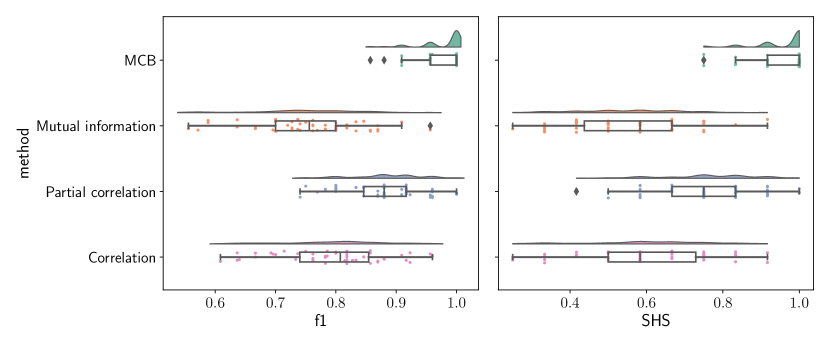
Figure 1: Raincloud plots of the distributions of (left) F1 score and (right) SHS, obtained by the tested methods over $50$ synthetic data sets. For readability, we omit the results by DTF and PDC.

Figure 1 depicts the results obtained by the considered methods over the $50$ synthetic data sets. Here, we omit DTF and PDC for readability reasons, as their performance is quite low (Section F.1 shows the complete figure). Our methodology outperforms the baselines on both metrics. Specifically, the kernel density estimate (KDE) corresponding to our method is highly concentrated around the maximum value. Conversely, the KDEs associated with mutual information and Pearson’s correlation exhibit high dispersion. The results obtained from these two methods are statistically equivalent, as expected. Finally, the second most effective method is partial correlation. In a linear setting, this method benefits from information regarding conditional dependence.

6 Analysis of resting-state fMRI data

We study the data set introduced by Termenon et al. (2016), which encompasses a large sample of rs-fMRI data, publicly released as part of the HCP (Smith et al., 2013). The data set comprises rs-fMRI recordings from $100$ healthy adults, with each subject undergoing two rs-fMRI acquisitions on separate days. During the acquisition, subjects were instructed to lie with their eyes open, maintaining a relaxed fixation on a white cross against a dark background. They were asked to keep their minds wandering and remain awake throughout the session.

Accordingly, we have $S=100$ individual data sets, for two separate days. The parcellation scheme divides the brain into $89$ ROIs. We separately analyze the ROIs of the left hemisphere and those of the right hemisphere. This approach prevents signal averaging across brain regions corresponding to different hemispheres. Consequently, each hemisphere contains $K=45$ ROIs, with the vermis region being common to both. Additionally, each acquisition session has a duration of $14$ minutes and $24$ seconds, which results in a total of $N=1200$ timestamps. For further details regarding the data source, we refer the interested reader to Termenon et al. (2016).

Analysis of the MCBs. We apply our methodology and the baseline methods considered in Section 5 to this dataset. To retrieve the brain connectivity backbone according to the baselines, we use the same approach as in Section 5, which is detailed in Section F.1. For the multiscale decomposition performed by MS-CASTLE, we use the SWT with Daubechies wavelets with filter length equal to $10$, consistently with the approach used by Termenon et al. (2016). The set of $p$-persistent arcs $\mathcal{U}_{p}$ is constructed by selecting arcs that are present in more than $p=80$ individuals on each day of the acquisition. This criterion is also used within the application of the baselines methods to decide whether an arc has to be added to the connectivity backbone. Furthermore, we set the threshold parameter to $\tau=0.2$, for all the methods, after having explored the effect of $\tau$ on the cardinality of the arc sets of the individual multiscale DAGs (see Section F.2). Finally, we evaluate the statistical significance of the arcs within the MCB retrieved by our method via a bootstrap with resampling. More in detail, starting from the $200$ multiscale DAGs learned by MS-CASTLE, we create $100$ samples, where each sample consists of $200$ multiscale DAGs obtained by means of bootstrap. At this point, we retrieve the MCB corresponding to each sample, and we retain the arcs that are associated with weights statistically different from zero at $10\%$ level within the $\{\widehat{G}^{s}_{\widehat{\mathcal{A}}_{p}}\}$.

Baseline methods retrieve dense networks for both the right and left hemispheres, and it is challenging to draw any conclusion from the results. Due to space constraints, the corresponding connectivity backbones are given in Section F.3.

Conversely, our methodology produces sparse MCBs for both hemispheres, provided in Figure 7 in Section F.3 for space reasons. Our findings suggest that finer scales are characterized by more complex structures. Here ROIs associated with different functionalities interact. Conversely, at coarser scales causal interactions mainly occur between ROIs associated with the same functionalities. Furthermore, as expected nodes related to processing of external stimuli (i.e., visual, auditory, speech, and language) appear and interact at the first three scales. Conversely, nodes associated with higher-level cognitive functions and emotions appear throughout the considered scales, as expected in resting-state.

Specifically, our findings are the following:

• The occipital lobe consistently plays a central role within the visual network (VN) across various frequency scales. This suggests its fundamental role in visual processing (Utevsky et al., 2014; Cunningham et al., 2017).

• The superior parietal gyrus, crucial for sensory integration and attention, has widespread impacts. It influences the precuneus in the default mode network (DMN), indicating a link between sensory integration and self-awareness (Freedman and Ibos, 2018; Tamietto et al., 2015).

• The postcentral gyrus, primarily involved in somatosensory information processing, is a key node. At finer scales, it connects to the precentral gyrus, which governs voluntary motor movements, and further activates the middle frontal gyrus, involved in high-level cognitive functions (Johansen-Berg and Matthews, 2002; Brown, 2001).

• Nodes in the frontal regions (e.g., orbital surface of the inferior frontal gyrus, lateral surface of the superior frontal gyrus) have significant impacts. They govern emotion processing, cognitive flexibility, decision-making, and cognitive control (Boisgueheneuc et al., 2006; Rolls, 2000).

• The middle temporal gyrus, involved in various functions like language, memory, and cognition (Davey et al., 2016), influences other temporal regions, including the superior temporal gyrus and the temporal pole (Allison et al., 2000; Diveica et al., 2021). Additionally, several works in neuroscience point out a link between abnormalities in these brain regions and the autism disorder spectrum (see Jou et al., 2010; Sato et al., 2017 and references therein).

• The nature of brain connectivity is dynamic, with certain nodes serving as common causes across different networks and frequency scales. The multiscale causal analysis points out the presence of bi-directional connections (e.g., between the precentral gyrus and the postcentral gyrus), and effectively locates the occurrence of the change of direction of the arcs in the frequency domain. Additionally, it suggests two regimes in causal interactions: (i) at higher frequencies, sensory information is a key driver in the network (Mantini et al., 2007; Smith et al., 2009), together with the high-level cognitive function of the lateral surface of the superior frontal gyrus; (ii) at lower ones the shared brain activity is driven by the nodes of the DMN, specifically the lateral surface of the superior frontal gyrus and the precuneus, which contribute to processes related to self-awareness, introspection, and self-referential thinking (Raichle et al., 2001; Uddin et al., 2008).

The detailed analysis organized per scales is given in Section F.3.

Comparison with the SCBs. An interesting point concerns the comparison between the MCBs and the SCBs that can be obtained by the application of the backbone search procedure (equipped with bootstrap with resampling) to subject-specific single-scale causal graphs.

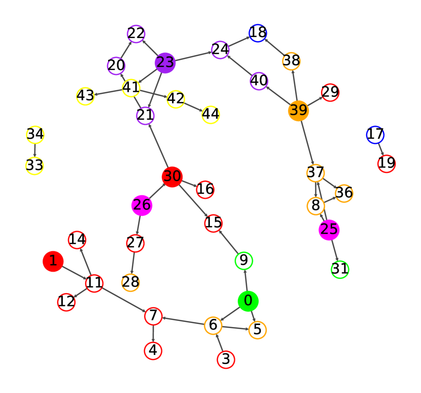
(a) Left

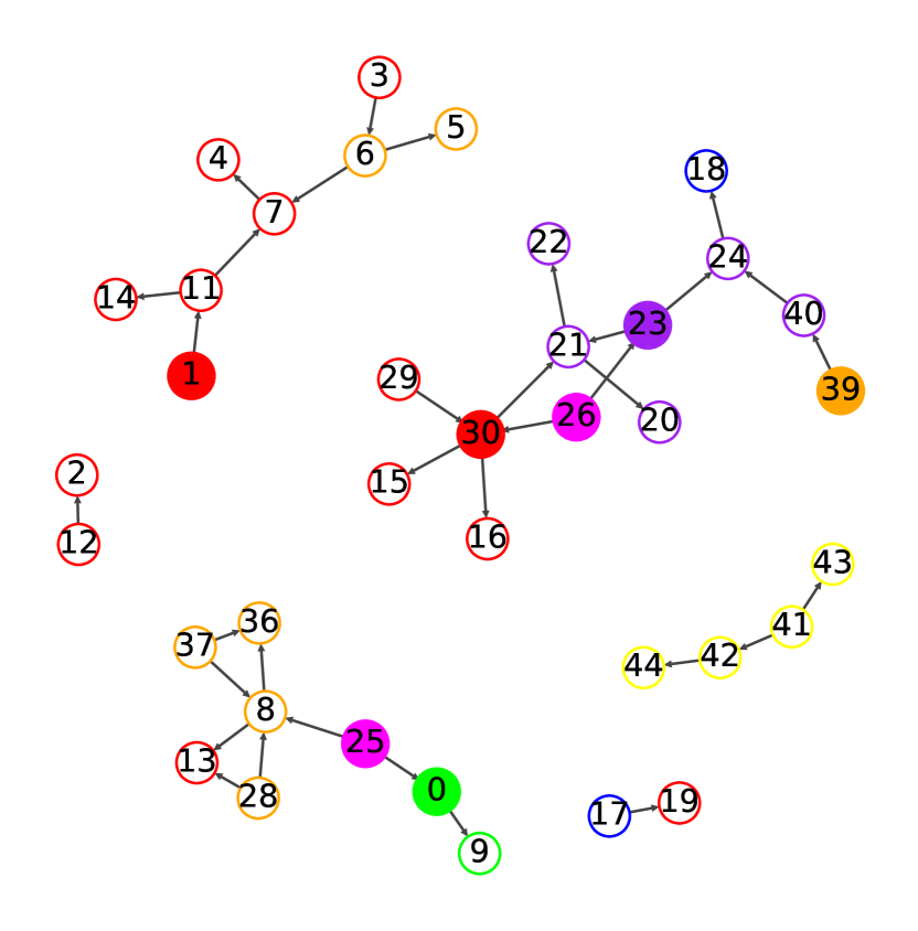
(b) Right

Figure 8: SCBs for (8) the left and (8) the right hemispheres. Color-filled nodes are the main drivers within the MCBs in Figure 7.

The SCBs provided in Figure 8 in Section F.4 confirm the importance of the regions highlighted by the multiscale analysis, which also appear to be the main drivers in this analysis. However, while the MCBs allow us to study causal structures in distinct frequency bands, thus enabling us to locate the predominance of certain brain activities over others in the frequency domain and detect structural changes, in the SCBs the information is aggregated. As an example, consider the causal connection from the superior parietal gyrus (node $26$) to the precuneus (node $30$) in Figure 8. Looking at the MCBs in Figures 7, 7, 7, 7 and 7, we see that this connection only occurs at the first three time scales, i.e., frequencies greater than $0.087$ Hz. Moreover, the aggregation of information within the SCBs also leads to the loss of certain connections, such as the bidirectional one between the precentral gyrus (node $0$) and the postcentral gyrus (node $25$). These regions belong to the sensory-motor network (Mantini et al., 2007; Smith et al., 2009), and the bi-directionality of this causal relation confirms that they collaborate to control and sense movements.

Causal fingerprinting. Finally, an intriguing point concerns the individual variability of multiscale causal structures, that we name causal fingerprinting. This concept relates to the well-studied functional connectivity fingerprinting, i.e., the usefulness of functional connectivity in identifying subjects within large groups (Miranda-Dominguez et al., 2014; Finn et al., 2015; Liu et al., 2018; Elliott et al., 2019). Let us indicate with $G^{i}_{h,t}$ the individual multiscale DAG learned by MS-CASTLE, and corresponding to the hemisphere $h$ of subject $i$ at acquisition $t$, where $h\in\{\mathrm{left},\mathrm{right}\}$, $t\in\{t_{1},t_{2}\}$, and $i\in[S]$. The tested hypothesis is that the similarity between $G^{i}_{h,t_{1}}$ and $G^{i}_{h,t_{2}}$ is statistically different from the similarity between $G^{i}_{h,t_{1}}$ and $G^{j}_{h,t_{1}}$ for $j\in[S-1]$. Mathematically, this can be expressed as $\mathrm{H}_{0}:\mathrm{J}(G^{i}_{h,t_{1}},G^{i}_{h,t_{2}})=\mathrm{J}(G^{i}_{h,t_{1}},G^{j}_{h,t_{1}})$, where $\mathrm{J}$ represents the Jaccard score used for measuring the similarity between individual multiscale DAGs (Jaccard, 1912). Statistical significance is assessed by the two-sample Cramér-von Mises (Anderson, 1962) test at $0.1\%$ level, after applying the Bonferroni correction (Bonferroni, 1936).

Figure 2: Comparison of the Jaccard score between the individual multiscale DAGs corresponding to the same hemisphere and the same subject at different timestamps (acquisitions) $t_{1}$ and $t_{2}$, to the Jaccard score between the individual multiscale DAGs corresponding to the same hemisphere of different subjects at the same timestamp. The analysis is conducted at different hard-thresholding levels $\tau\in(0,1]$.

The results are depicted in Figure 2. The individual multiscale DAGs for the same subject are indeed more similar than those of different subjects across various hard-thresholding levels $\tau$. The null hypothesis is rejected at each $\tau$. Thus, individual multiscale DAGs can effectively differentiate between different subjects within large groups, supporting the existence of causal fingerprinting.

7 Conclusions

In this paper, we investigate the discovery of an MCB in brain dynamics across individuals. We propose a principled methodology that leverages recent advances in multiscale causal structure learning, optimizing the balance between model fit and complexity. Our approach outperforms a baseline based on canonical functional connectivity in learning the MCB, as demonstrated on synthetic data. Applying this method to real-world resting-state fMRI data reveals sparse MCBs in both the left and right brain hemispheres. The multiscale nature of our approach allows us to extract that high-level cognitive functions drive causal dynamics at low frequencies, while sensory processing nodes are relevant drivers at higher frequencies. Our analysis confirms the presence of a causal fingerprinting of brain connectivity among individuals, from a causal standpoint. Future work should be devoted to studying MCBs by using data from individuals performing various tasks and individuals with neurological disorders. Discovering MCBs in these contexts is crucial for understanding how brain dynamics operate when the brain is subject to stimuli, and how they are affected by neurological disorders. Such studies can lead to insights that may facilitate the development of targeted interventions and therapies for cognitive enhancement or the treatment of neurological conditions.

Appendix A Proof of Lemma 1

See 1

Proof.

Let us consider the signal $\mathbf{x}^{s}_{i}\in^{N}$, and define $\mathbf{c}_{i}^{s,0}=\tilde{\mathbf{x}}_{i}^{s,0}=\mathbf{x}^{s}_{i}$. Consider an orthogonal wavelet family defined by the high-pass and low-pass filters, $\mathbf{h}\in^{L}$ and $\mathbf{g}\in^{L}$, respectively. Hence the we have that

$$\tilde{x}_{i}^{s,j}[n] =\sum_{l=0}^{L-1}h[l]c_{i}^{s,j-1}[n+l],$$

$$c_{i}^{s,j}[n] =\sum_{l=0}^{L-1}g[l]\tilde{x}_{i}^{s,j-1}[n+l].$$

Thus, given Assumption 1, $\tilde{x}_{i}^{s,j}[n]$ and $c_{i}^{s,j}[n]$ are distributed according to a zero-mean Gaussian distribution, since linear combinations of i.i.d. Gaussian variables from the $i$-th dimension of $N(\mathbf{0},\boldsymbol{\Omega}^{s})$. ∎

Appendix B Arc addition

Let us consider as in Section 4 that the last added $p$-persistent arc for the scale $j$ is $q\rightarrow r$, $u_{qr}^{j}$. Hence, given the decomposability of the score in (8), we only have to update the family score for the child node $v$ given in (9). Accordingly, we only consider the $p$-persistent arcs $u_{lr}^{j}\in\mathcal{U}_{p}^{j}$ ending in $r$, where $\mathcal{U}_{p}^{j}$ no longer contains previously evaluated arcs. Specifically, for each of these $p$-persistent arcs, we compare $\mathrm{M}_{0}$ and $\mathrm{M}_{1}$ by means of the following linear regression model

$$\tilde{\mathbf{x}}^{s,j}_{v}=b_{lr}^{s,j}\tilde{\mathbf{x}}^{s,j}_{l}+\sum_{y\in\mathcal{P}^{s,j}_{r}}b_{yr}^{s,j}\tilde{\mathbf{x}}^{s,j}_{y}+\mathbf{z}^{s,j}_{r},\quad\forall s\in[S],$$ (10)

where $\mathcal{P}^{s,j}_{r}$ is the current parent set of the node $r$, at scale $j$ for individual $s$. Hence, we compute the least-squares estimates for the regression coefficients, for all the $S$ individuals in a parallel fashion. $\mathrm{RIC}^{\mathrm{M}_{0}}$ corresponds to the case in which the log-likelihoods of all the individuals are evaluated at the least-squares estimates with $b_{lr}^{s,j}=0$, whereas $\mathrm{RIC}^{\mathrm{M}_{1}}$ to the case in which $b_{lr}^{s,j}\neq 0$. At this point, each $p$-persistent arc $u_{lr}^{j}$ ending in $r$ is associated with a $\Delta_{\mathrm{RIC}}^{j}=\sum_{s\in[S]}\Delta_{\mathrm{RIC}}^{s,j}$. Subsequently, we add to $\widehat{\mathcal{A}}_{p}^{j}$ the $p$-persistent arc $u_{lm}^{j}\in\mathcal{U}_{p}^{j}$ associated with the lowest $\Delta_{\mathrm{RIC}}$, and that does not induce any cycle in the solution. Due to independence, this procedure can be run in parallel over the time scales $j\in[J]$.

Appendix C Computational cost

In our setting $N>K$ (cf, Section 6). At each step, we have to update the family score in (9) for the child node of the last added $p$-persistent arc. Let’s say that the child node is $r$, and it has $K^{s,j}<K-1$ parents for the scale $j$ and individual $s$. According to Appendix B, for evaluating the candidate $p$-persistent arc $u_{lr}^{j}$, we need to compute the least-squares estimates in (10). The cost of evaluating the least-squares estimates of the regression coefficients for all the candidate $p$-persistent arcs $u_{lr}^{j}$ ending in $r$ is asymptotically $\mathcal{O}(N(K^{s,j}+1)^{2})$. Indeed, we first compute the pseudo-inverse of $\widetilde{\mathbf{X}}^{s^{\top}}\in^{N\times(K^{s,j}+1)}$ using SVD decomposition, requiring $\mathcal{O}(N(K^{s,j}+1)^{2})$ flops. Then, we multiply the pseudo-inverse by $\tilde{\mathbf{x}}^{s,j}_{r}\in^{N}$, requiring a cheaper cost, i.e., $\mathcal{O}(2(K^{s,j}+1)N)$. Since we can parallelize over the individuals and over the time scales, the overall cost for the update of the family score for each candidate $p$-persistent arc is $\mathcal{O}(N(K^{\prime}+1)^{2})$, where $K^{\prime}=\max_{s,j}K^{s,j}$. Now, let us define $U=\max_{j}|\mathcal{U}_{p}^{j}|$. Since we might have more than one $p$-persistent arc to evaluate, the total cost for evaluating all the least-squares estimated is asymptotically upper-bounded by $\mathcal{O}(UN(K^{\prime}+1)^{2})$.

At this point, we compute $\Delta_{RIC}^{j}$ for the candidate $p$-persistent arcs $u_{lr}^{j}$, which requires to evaluate (9) given the least-squares estimates. In particular, here the most demanding operation is the computation of the quadratic term, which is upper-bounded by $\mathcal{O}((2N+3)K^{\prime})$. Again, considering that we might have multiple $p$-persistent arcs, the overall cost for this step is $\mathcal{O}(U(2N+3)K^{\prime})$.

Subsequently, we select the arc having the minimum absolute $\Delta_{RIC}^{j}$, with a cost linear in $|\mathcal{U}_{p}^{j}|$. Finally, we check the acyclicity of the $j$-th layer of MCB with arc set $\widehat{\mathcal{A}}_{p}^{j}$, requiring $\mathcal{O}(|\widehat{\mathcal{A}}_{p}^{j}|)$ flops. Based on this analysis, the most demanding step is the computation of least-squares estimates for updating the family scores, which at the beginning is done for all the $p$-persistent arcs in $\mathcal{U}_{p}^{j}$, in parallel over $j\in[J]$.

Appendix D Hyper-parameters

Method	Persistence $p$	Hard-thresholding $\tau$	$\ell_{1}$-regularization strength, $\lambda$
MCB	65	0.15	0.01
Mutual information	60	0.05	N/A
Pearson’s correlation	65	0.15	N/A
Partial correlation	65	0.25	N/A
DTF	60	0.0	N/A
PDC	60	0.0	N/A

Table 1: The table shows the values for the relevant hyper-parameters used in the results depicted in Figures 1 and 3.

The values for the relevant hyper-parameters used in the empirical assessment on synthetic data are provided in Table 1. The $\ell_{1}$-regularization strength is only used by SS-CASTLE.

Appendix E Metrics

We define the considered metrics similarly to Zheng et al. (2018). Specifically, we denote:

• $\mathrm{cp}$ as the count of true positive arcs, i.e., the number of arcs present in the ground truth.

• $\mathrm{cn}$ as the count of true negative arcs, i.e., the number of arcs that are absent in the ground truth.

• $\mathrm{tnnz}$ as the total number of arcs in the ground truth.

• $\mathrm{nnz}$ as the total number of estimated arcs.

• $\mathrm{tp}$ as the count of true positives, i.e., the number of estimated arcs present in the ground truth and with the correct direction.

• $\mathrm{r}$ as the count of reversed arcs, i.e., the number of learned arcs present in the ground truth but with the opposite direction.

• $\mathrm{fp}$ as the count of false positives, i.e., the number of learned extra arcs not present in the undirected skeleton of the ground truth.

• $\mathrm{e}$ as the count of missing arcs, i.e., the number of arcs in the skeleton of the learned graph that are extra compared to the skeleton of the ground truth.

• $\mathrm{m}$ as the count of extra arcs, i.e., the number of arcs in the skeleton of the learned graph that are missing compared to the skeleton of the ground truth.

With these definitions in place, we can calculate the following metrics:

• False Discovery Rate (FDR) is given by $\mathrm{fdr}=(\mathrm{r}+\mathrm{fp})/\mathrm{nnz}$.

• True Positive Rate (TPR) is calculated as $\mathrm{tpr}=\mathrm{tp}/\mathrm{cp}$.

• False Positive Rate (FPR) is determined as $\mathrm{fpr}=(\mathrm{r}+\mathrm{fp})/\mathrm{cn}$.

Consequently, the F1-score is equal to $2\cdot\frac{(1-\mathrm{fdr})\mathrm{tpr}}{1-\mathrm{fdr}+\mathrm{tpr}}$, the normalized Structural Hamming Distance (nSHD) is computed as $\frac{(\mathrm{r}+\mathrm{m}+\mathrm{e})}{\mathrm{tnnz}}$, and the structural Hamming similarity is $\mathrm{SHS}=1-\mathrm{nSHD}$.

Appendix F Additional results

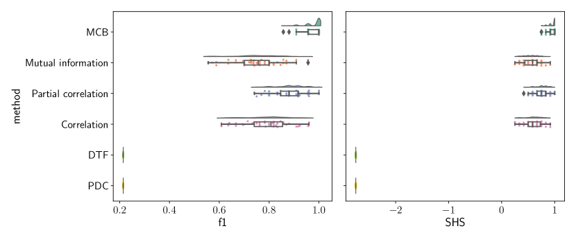
Figure 3: Rain plots depicting the (left) F1 score and (right) SHS, obtained by the considered methods over $50$ synthetic data sets.

F.1 Synthetic data

Here we dive into the procedure used for testing the considered methods on synthetic data, and we provide additional discussion about the comparison.

Baselines. As shown in Section 5, we compare the proposed methodology with widely used measures of functional connectivity in terms of F1 score and structural Hamming similarity. In detail, among the connectivity measures outlined in Section 1, we consider (i) DTF and PDC among the existing directed measures, and (ii) Pearson’s correlation, partial correlation, and mutual information among the undirected ones. We apply these connectivity measures to each subject $s\in[S]$ in order to retrieve individual brain connectivity networks, where each node corresponds to one of the ten synthetically generated time series.

In the case of undirected measures, the resulting individual brain connectivity networks are undirected. For subject $s$, the weight of the arc between nodes $l$ and $m$ represents the value of the considered connectivity measure when it is computed by taking as input the time series corresponding to nodes $l$ and $m$ associated with subject $s$. In the case of directed measures, the obtained networks are directed, but not necessarily acyclic. In addition, given two time series, DTF and PDC evaluate the statistical dependence by analyzing the spectral Granger causality. In brief, DTF and PDC consider $F\in\mathbb{N}$ different frequencies, and for each $f\in[F]$, they return the measure of statistical dependence between the time series (refer to Kaminski and Blinowska, 1991; Baccalá and Sameshima, 2001 for details). This means that, by considering all the $K$ time series, we obtain $K$ by $K$ connectivity matrices for every $f$. Let us denote this matrix with $\mathbf{D}^{s,f}$. Now, in order to obtain the weight of the arcs for the individual brain connectivity networks, we stack the connectivity matrices $\mathbf{D}^{s,f}$ along the frequency dimension, i.e., along $f$, thus obtaining a $K$ by $K$ by $F$ tensor $\{\mathbf{D}^{s,f}\}_{f\in[F]}$. Hence, to aggregate this information in a matrix $\widetilde{\mathbf{D}}^{s}\in^{K\times K}$, we compute the $\ell_{2}$-norm along the tube dimension of the tensor corresponding to the frequency index, i.e., $f$. At this point, we obtain the weighted adjacency of the brain connectivity network for the $s$-th individual (and thus the weights for the arcs), by computing $\widehat{\mathbf{D}}^{s}=\mathbf{R}^{s}\widetilde{\mathbf{D}}^{s}\mathbf{R}^{s}$, where $\mathbf{R}^{s}\in^{K\times K}$ is the diagonal matrix with entries $[\widetilde{\mathbf{D}}^{s}]_{ii}^{-1/2},\,\forall i\in[K]$.

Once we have obtained all the brain connectivity networks, we apply hard-thresholding to retain only those arcs whose absolute weights are greater than a hyper-parameter $\tau\in_{+}$. The same hyper-parameter is also used for pruning the single-scale causal DAGs returned by the single-scale counterpart of MS-CASTLE, i.e., SS-CASTLE (D’Acunto et al., 2023).

At this point, for each baseline, we consider as an estimate of $\mathcal{A}_{p}$ the set of connections that occur in more than $p$ individual brain connectivity networks, where $p<S,\,p\in\mathbb{N}$. Our approach, instead, uses the same hyper-parameter $p$ to individuate the $p$-persistent arcs in Definition 2 composing $\mathcal{U}_{p}$. Then, the score-based search procedure in Section 4 is run over the pruned single-scale individual causal DAGs to retrieve the $\mathcal{A}_{p}$. Details concerning the fine-tuning of $\tau$ and $p$ are given in Appendix D.

Additional comparison with baselines. Figure 3 depicts the results obtained by the considered methods over $50$ synthetic data sets. In addition to the discussion provided in Section 5, here we see that both DTF and PDC fail in backbone discovery, returning the fully connected single-scale causal backbone (SCB) in every case. We believe that there are two reasons behind this behavior. Firstly, the underlying ground truth causal structure contains only instantaneous connections, while DTF and PDC are based on the spectral formulation of Granger causality, which pertains to lagged causal connections. Secondly, according to both methods, a relationship between two signals is identified if the measured value is different from zero for at least one frequency. Consequently, noisy estimates can lead to the presence of spurious arcs.

F.2 Analysis of the cardinality of individual multiscale DAGs

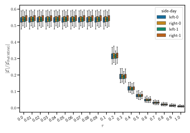
Figure 4: The figure depicts the behavior of the cardinality of the individual multiscale causal DAGs for the two hemispheres and different days of acquisition along $\tau$, normalized by the number of arcs of the fully connected individual multiscale causal DAG.

Figure 4 shows the impact of the hard-thresholding level $\tau$ on the cardinality of the arc set of the individual multiscale causal DAGs for the two hemispheres and different days of acquisition. To facilitate the interpretation of the plot, we normalize the cardinality of the arc sets by the number of arcs of the fully connected individual multiscale causal DAG, i.e., $(J\cdot N\cdot(N-1))/2$. As we see, $\tau=0.2$ is the first value (among those considered) that effectively reduces the cardinality of the arc sets. Accordingly, we use this value in the analysis given in Section 6.

F.3 Comparison with baselines and analysis of the resulting MCBs by scale

Node Number	Region	Macro-afferent Region	Related Functions
0	Precentral gyrus	Central	Motor network (Penfield and Boldrey, 1937)
1	Superior frontal gyrus	Frontal - Lateral	Cognitive functions, attention (Boisgueheneuc et al., 2006)
2	Superior frontal gyrus	Frontal - Orbital	Emotion, working memory (Zhao et al., 2020; Hu et al., 2016)
3	Middle frontal gyrus	Frontal - Lateral	Working memory, attention, memory (Ridderinkhof et al., 2004; Koechlin et al., 2003)
4	Middle frontal gyrus	Frontal - Orbital	Emotion, decision making (Zhao et al., 2020)
5	Inferior frontal opercular gyrus	Frontal - Lateral	Speech and language processing (Price, 2012)
6	Inferior frontal triangular gyrus	Frontal - Lateral	Speech and language processing, working memory (Price, 2012)
7	Inferior frontal gyrus	Frontal - Orbital	Emotion, decision making (Rolls, 2000)
8	Rolandic operculum	Central	Speech and language processing, working memory, attention (Meyer and Jäncke, 2006)
9	Supplementary Motor Area	Frontal - Medial	Motor network (Nachev et al., 2008)
10	Olfactory cortex	Frontal - Orbital	Olfaction (Gottfried, 2010)
11	Superior frontal gyrus	Frontal - Lateral	Default mode network (Uddin et al., 2008)
12	Superior frontal and rectus gyri	Frontal - Orbital	Emotion, decision making (Ray and Zald, 2012)
13	Insula	Insula	Emotion, self-awareness (Craig, 2009)
14	Anterior cingulate and paracingulate gyri	Limbic	Emotion, decision making (Bush et al., 2000)
15	Median cingulate and paracingulate gyri	Limbic	Emotion, pain processing (Vogt, 2005)
16	Posterior cingulate gyrus	Limbic	Default mode network (Buckner et al., 2008)
17	Hippocampus	Limbic	Memory formation, memory retrieval (Eichenbaum, 2017)
18	Parahippocampal gyrus	Limbic	Memory formation, memory retrieval (Gandolla et al., 2014)
19	Amygdala	Subcortical Gray Nuclei	Emotional processing (LeDoux, 2007)
20	Calcarine fissure and surrounding cortex	Occipital - Medial and inferior	Primary visual (Wandell and Winawer, 2011)
21	Cuneus	Occipital - Medial and inferior	Visual processing (Wandell and Winawer, 2011)
22	Lingual gyrus	Occipital - Medial and inferior	Object recognition (Grill-Spector and Malach, 2004)
23	Occipital gyrus	Occipital - Lateral	Visual processing (Wandell and Winawer, 2011)
24	Fusiform gyrus	Occipital - Medial and inferior	Face and object recognition (Kanwisher et al., 1997)
25	Postcentral gyrus	Central	Somatosensory network (Iwamura et al., 1994)
26	Superior parietal gyrus	Parietal - Lateral	Sensory integration, attention (Corbetta and Shulman, 2002)
27	Inferior parietal gyrus	Parietal - Lateral	Default mode network, attention (Caspers et al., 2006)
28	Supramarginal gyrus	Parietal - Lateral	Language processing, working memory, memory retrieval (Rushworth et al., 2003)
29	Angular gyrus	Parietal - Lateral	Default mode network (Seghier, 2013)
30	Precuneus	Parietal - Medial	Default mode network (Raichle et al., 2001)
31	Paracentral lobule	Frontal - Medial	Motor network (Picard and Strick, 1996)
32	Caudate nucleus	Subcortical Gray Nuclei	Motor control, cognitive control (Graybiel, 2000)
33	Putamen	Subcortical Gray Nuclei	Motor control, motor learning (Haber and Knutson, 2010)
34	Pallidum	Subcortical Gray Nuclei	Motor control (Kita, 2007)
35	Thalamus	Subcortical Gray Nuclei	Sensory processing, motor control, cognitive functions (Sherman and Guillery, 2002)
36	Heschl gyrus	Temporal - Lateral	Auditory processing, language processing (Smith et al., 2011)
37	Superior temporal gyrus	Temporal - Lateral	Auditory processing, language processing, memory, Cognitive functions (Howard et al., 2000)
38	Temporal pole	Temporal pole	Auditory processing, language processing, memory retrieval, episodic memory (Olson et al., 2007, 2013)
39	Middle temporal gyrus	Temporal - Lateral	Auditory processing, language processing, memory retrieval, episodic memory (Davey et al., 2016)
40	Inferior temporal gyrus	Temporal - Lateral	Visual processing, visual memory, cognitive functions (Grill-Spector and Malach, 2004)
41	Cerebellum I II	Cerebellum	Motor control, coordination (Ito, 2008)
42	Cerebellum III - VI	Cerebellum	Motor control, coordination (Ito, 2008)
43	Cerebellum VII - X	Cerebellum	Motor control, coordination (Ito, 2008)
44	Vermis	Cerebellum	Motor control, coordination (Coffman et al., 2011)

Table 2: The table shows the number of the node corresponding to each ROI. In addition, we report the macro-afferent regions.

(a) Pearson’s correlation

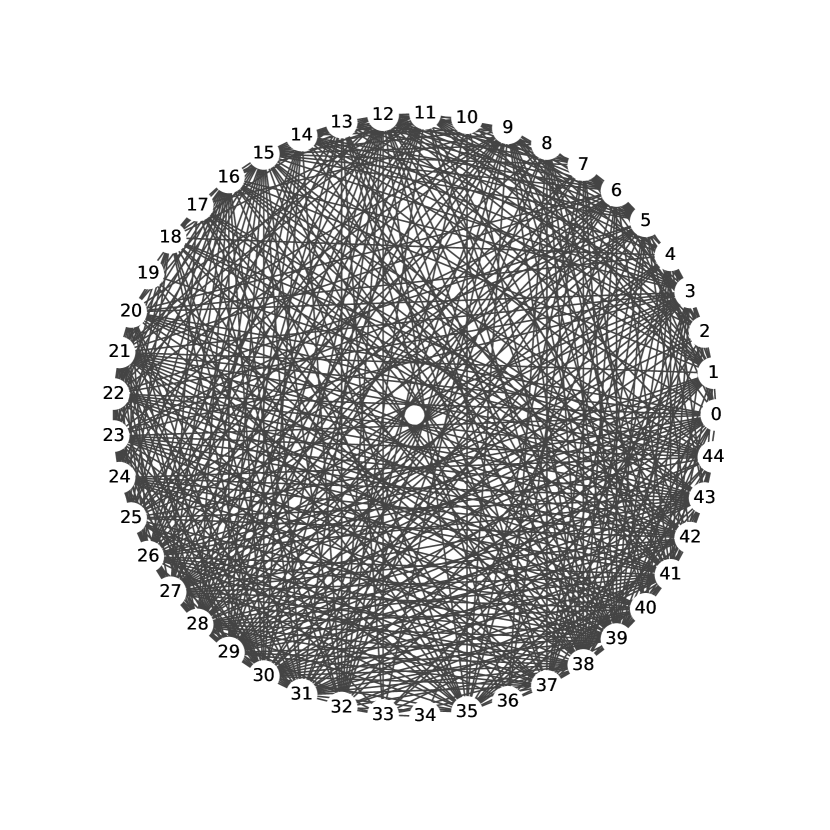
(b) Partial correlation

(c) Mutual information

(d) DTF

(e) PDC

Figure 5: Connectivity backbones retrieved by the considered baseline methods for the left hemisphere. ROIs numbering in Table 2.

(a) Pearson’s correlation

(b) Partial correlation

(c) Mutual information

(d) DTF

(e) PDC

Figure 6: Connectivity backbones retrieved by the considered baseline methods for the right hemisphere. ROIs numbering in Table 2.

Figures 5 and 6 show that the baseline methods retrieve dense networks for both the right and left hemispheres. Consequently, these methods suggest that the common connectivity matrix involves all the ROIs, in an intricate fashion.

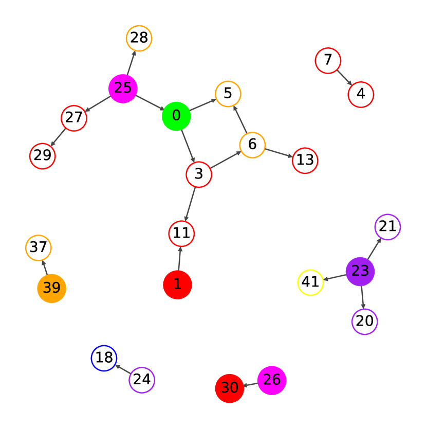
(f) Scale $1$, left

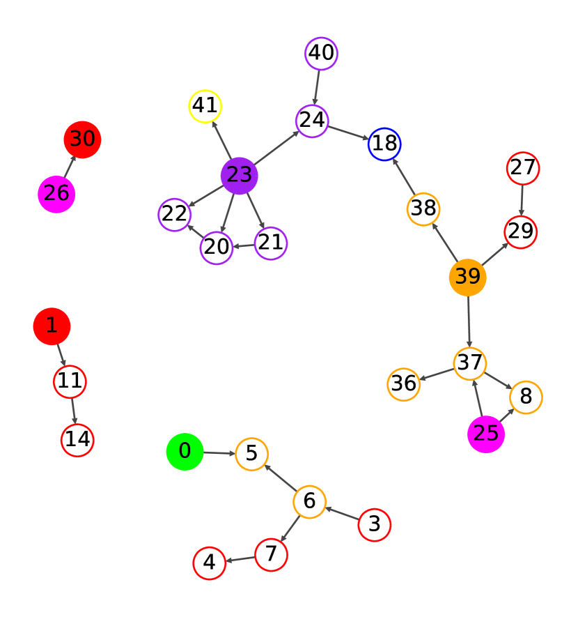
(g) Scale $2$, left

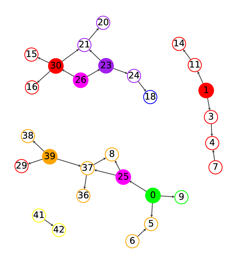
(h) Scale $3$, left

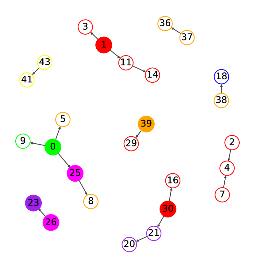
(i) Scale $4$, left

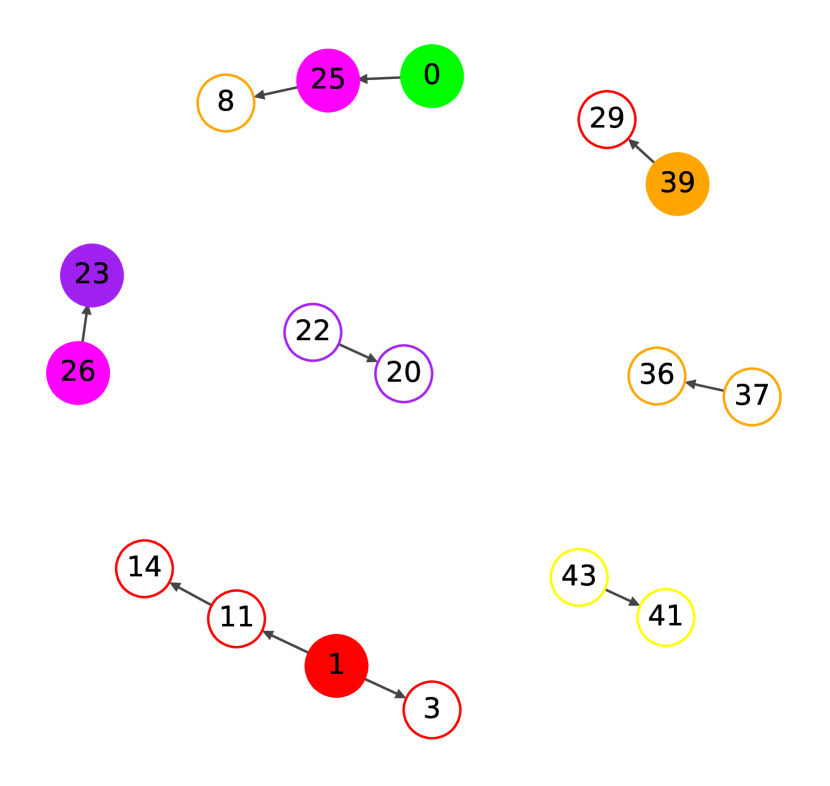
(j) Scale $5$, left

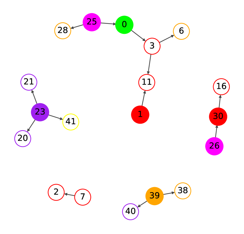
(k) Scale $1$, right

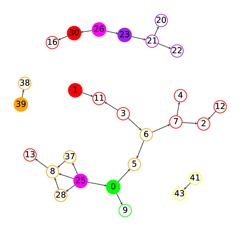
(l) Scale $2$, right

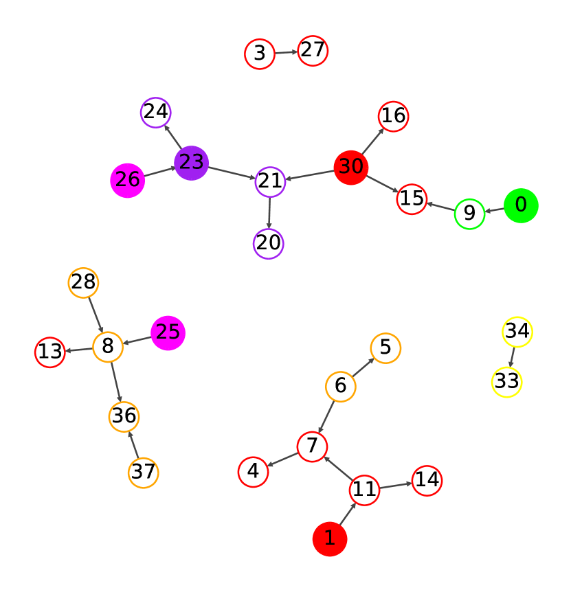
(m) Scale $3$, right

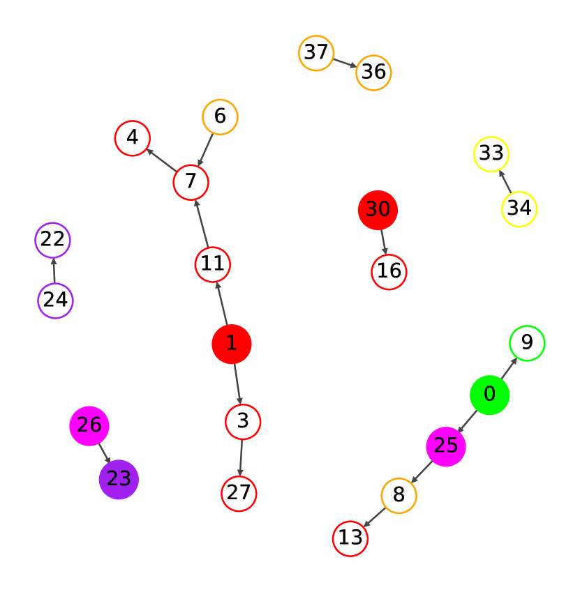
(n) Scale $4$, right

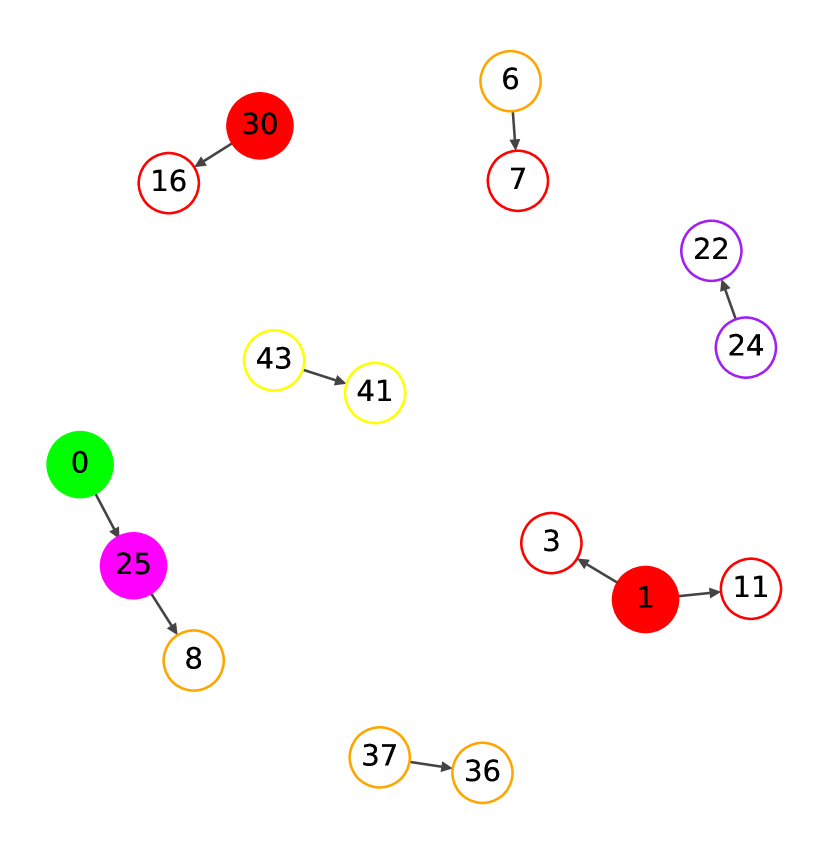
(o) Scale $5$, right

Figure 7: MCBs for the left and the right hemispheres. The main driver nodes are color-filled. ROIs numbering in Table 2.

Conversely, our method proposes sparse MCBs, which allow to extract meaningfull information from data. Figure 7 depicts the obtained results for the left (depicted on top) and the right hemispheres (bottom). We plot separately the causal backbones for distinct time scales, from the finest on the left to the coarsest on the right. Additionally, to better visualize the results, we use the following color coding inspired by the ROIs functions given in Table 2 :

• Red for ROIs corresponding to cognitive functions, attention, emotion, and decision making;

• Orange for those related to auditory processing, speech and language processing, and memory;

• Blue for those concerning memory formation and memory retrieval;

• Pink for those associated with sensory integration and somatosensory;

• Purple for the ROIs within the visual network and related to the visual memory;

• Green for those within the motor network;

• Yellow for those regarding the motor control and the posture.

We provide below a detailed discussion of the obtained results, organized by scales.

Scale 1 $([0.694-0.347]\mathrm{Hz}).$ Looking at the MCBs in Figures 7 and 7, corresponding to the finest scale, we observe a central role of the occipital lobe ($23$) within the visual network (VN), for both hemispheres. It is also interesting to see the impact of the superior parietal gyrus ($26$), linked to sensory integration and attention (Corbetta and Shulman, 2002; Culham and Kanwisher, 2001 and references therein), on the precuneus ($30$), central node of the default mode network (DMN, Raichle et al., 2001; Buckner et al., 2008). This means that the integration of sensory information from different modalities, such as proprioception and vision, activates the self-awareness and self-referential processing of $30$. Continuing on this line, we see that the postcentral gyrus ($25$), primarily involved in processing somatosensory information (Iwamura et al., 1994; Disbrow et al., 2000), plays an important role. Specifically, it has an impact on the precentral gyrus ($0$), responsible for the planning and execution of voluntary motor movements (Penfield and Boldrey, 1937; Rizzolatti and Luppino, 2001), which then activate the middle frontal gyrus ($3$), involved in higher-order cognitive processes, such as decision-making Ridderinkhof et al. (2004); Koechlin et al. (2003). Furthermore, $25$ is shown to cause the activity of the supramarginal gyrus ($28$), which is involved in sensorimotor integration and helps to bridge the gap between sensory perception and motor action (Rushworth et al., 2003). We also notice, on the left hemisphere, an impact on the parietal inferior gyrus ($27$), involved in cognitive processes (Caspers et al., 2006). We attribute to this connection the same meaning as $26\rightarrow 30$. In addition, we see that the inferior frontal gyrus ($7$), associated in both hemispheres to emotion processing (Rolls, 2000 and references therein), impacts the middle frontal ($4$) and superior frontal ($2$) orbital gyri, involved in emotion regulation (Zhao et al., 2020 and references therein) and cognitive functions (Hu et al., 2016), respectively. Finally, the middle temporal gyrus ($39$), which is involved in language and visual processing but also in episodic memory and higher-level cognition (Davey et al., 2016; Briggs et al., 2021), is reported to influence the activity of the superior temporal gyrus ($37$), related to auditory and language-related functions (Howard et al., 2000), and the temporal pole ($38$) which is linked to emotion, memory and social cognition (Olson et al., 2007, 2013).

Scale 2 $([0.347-0.174]\mathrm{Hz}).$ Looking at the MCBs in Figures 7 and 7, corresponding to the second finest scale, we still observe the key role of the $23$ within the VN, for both hemispheres. Interestingly, we have connections from $26$ to nodes belonging to the DMN, but also a causal link toward $23$ in the VN, thus acting as a common cause. Hence, here the integration of sensory information impacts visual processing as well. Furthermore, we see that the processing of somatosensory information done by $25$ is a common cause for the planning and execution of voluntary motor movements, the sensorimotor integration, and auditory and language-related functions. Among the red nodes, we see again the central role of $7$ within the orbital surface of the frontal lobe. Also, it is interesting to see that the triangular part of the inferior frontal gyrus ($6$) mediates the effect of $3$ on $7$. This is consistent with the fact that the three nodes belong to the frontal executive network, which enables cognitive flexibility, decision-making, planning, inhibition of irrelevant information, and goal-directed behavior. Additionally, the superior frontal gyrus (lateral surface, $1$), involved in cognitive functions and attention (Boisgueheneuc et al., 2006), impacts the superior frontal gyrus (medial surface, $11$), which belongs to the DMN and thus relates to self-awareness and introspection. Finally, $39$ tends to cause the other regions within the temporal lobe.

Scale 3 $([0.174-0.087]\mathrm{Hz}).$ Referencing Figures 7 and 7, we see that also at this scale we can draw similar conclusions regarding the position of $23$ within the VN, and the common cause role of $25$ and $26$ related to sensory integration. Another analogy with the previous scales concerns nodes $1$ and $7$, which continue to cause the DMN activity and executive control functions. In addition, the causal graph corresponding to the left hemisphere highlights again the importance of $39$ within the temporal lobe, and its impact on the angular gyrus, part of the DMN. However, two distinctions from the previous scales emerge. The first concerns node $30$, which is a common cause for nodes in the DMN and the cuneus ($21$) of the VN. Specifically, $21$ processes visual information received from $23$, as also shown in the previous two scales. Hence, the precuneus provides context (e.g., episodic memory retrieval) to the cuneus, influencing how visual information is interpreted during mind-wandering. The second regards the relations between nodes $0$ and $25$, belonging to the sensory-motor network (Mantini et al., 2007; Smith et al., 2009), which is now reversed. The bi-directionality of this interaction confirms that the two regions collaborate to control and sense movements. Node $0$ sends signals to initiate the movement, and $25$ receives sensory feedback about the position and state of the body during the action. Then, this information is used to calibrate the subsequent voluntary action. Finally, in the left hemisphere, the central role of $39$ within the temporal lobe is further highlighted.

Scale 4 $([0.087-0.043]\mathrm{Hz}).$ The analysis of Figures 7 and 7 leads to conclusions similar to scale $3$. Nodes $1$ and $30$ are confirmed to be key drivers for high-level cognitive processes and visual processing. The impact of node $0$ on $25$ is reported, and the connections $26\rightarrow 23$, $39\rightarrow 29$ persist at this scale as well.

Scale 5 $([0.043-0.022]\mathrm{Hz}).$ Looking at Figures 7 and 7, we see that here the MCBs are sparser. While the V-structure $11\leftarrow 1\rightarrow 3$ and the chain $0\rightarrow 25\rightarrow 8$ persist in both hemispheres, the connections $30\rightarrow 16$ and $39\rightarrow 29$ appear only on the left one. In addition, the interaction between $30$ and $21$ disappears at this frequency band.

F.4 Graphical representation of the SCBs

In this appendix we provide the plots pertaining to the SCBs discussed in Section 6. In order to facilitate the comparison with the MCBs in Figure 7 we use the same numbering and color-coding for the ROIs.

References

- Felleman and Van Essen [1991] Daniel J Felleman and David C Van Essen. Distributed hierarchical processing in the primate cerebral cortex. Cerebral Cortex (New York, NY: 1991), 1(1):1–47, 1991.
- Biswal et al. [1995] Bharat Biswal, F Zerrin Yetkin, Victor M Haughton, and James S Hyde. Functional connectivity in the motor cortex of resting human brain using echo-planar MRI. Magnetic Resonance in Medicine, 34(4):537–541, 1995.
- Sporns et al. [2005] Olaf Sporns, Giulio Tononi, and Rolf Kötter. The human connectome: A structural description of the human brain. PLoS Computational Biology, 1(4):e42, 2005.
- Bullmore and Sporns [2009] Ed Bullmore and Olaf Sporns. Complex brain networks: Graph theoretical analysis of structural and functional systems. Nature Reviews Neuroscience, 10(3):186–198, 2009.
- Fox et al. [2005] Michael D Fox, Abraham Z Snyder, Justin L Vincent, Maurizio Corbetta, David C Van Essen, and Marcus E Raichle. The human brain is intrinsically organized into dynamic, anticorrelated functional networks. Proceedings of the National Academy of Sciences, 102(27):9673–9678, 2005.
- Wiener [1956] Norbert Wiener. The theory of prediction. Modern mathematics for engineers. New York, 165, 1956.
- Granger [1969] Clive WJ Granger. Investigating causal relations by econometric models and cross-spectral methods. Econometrica: Journal of the Econometric Society, pages 424–438, 1969.
- Schreiber [2000] Thomas Schreiber. Measuring information transfer. Physical Review Letters, 85(2):461, 2000.
- Ding et al. [2006] Mingzhou Ding, Yonghong Chen, and Steven L Bressler. Granger causality: Basic theory and application to neuroscience. Handbook of Time Series Analysis: Recent Theoretical Developments and Applications, pages 437–460, 2006.
- Guo et al. [2008] Shuixia Guo, Anil K Seth, Keith M Kendrick, Cong Zhou, and Jianfeng Feng. Partial Granger causality — Eliminating exogenous inputs and latent variables. Journal of Neuroscience Methods, 172(1):79–93, 2008.
- Kaminski and Blinowska [1991] Marcin Jan Kaminski and Katarzyna J Blinowska. A new method of the description of the information flow in the brain structures. Biological Cybernetics, 65(3):203–210, 1991.
- Baccalá and Sameshima [2001] Luiz A Baccalá and Koichi Sameshima. Partial directed coherence: A new concept in neural structure determination. Biological Cybernetics, 84(6):463–474, 2001.
- Blinowska [2011] Katarzyna J Blinowska. Review of the methods of determination of directed connectivity from multichannel data. Medical & Biological Engineering & Computing, 49:521–529, 2011.
- Bastos and Schoffelen [2016] André M Bastos and Jan-Mathijs Schoffelen. A tutorial review of functional connectivity analysis methods and their interpretational pitfalls. Frontiers in Systems Neuroscience, 9:175, 2016.
- Harrison et al. [2003] L Harrison, William D Penny, and Karl Friston. Multivariate autoregressive modeling of fMRI time series. NeuroImage, 19(4):1477–1491, 2003.
- Razi and Friston [2016] Adeel Razi and Karl J Friston. The connected brain: Causality, models, and intrinsic dynamics. IEEE Signal Processing Magazine, 33(3):14–35, 2016.
- Friston et al. [2003] Karl J Friston, Lee Harrison, and Will Penny. Dynamic causal modelling. NeuroImage, 19(4):1273–1302, 2003.
- Craddock et al. [2012] R Cameron Craddock, G Andrew James, Paul E Holtzheimer III, Xiaoping P Hu, and Helen S Mayberg. A whole brain fMRI atlas generated via spatially constrained spectral clustering. Human Brain Mapping, 33(8):1914–1928, 2012.
- Bassett and Sporns [2017] Danielle S Bassett and Olaf Sporns. Network neuroscience. Nature Neuroscience, 20(3):353–364, 2017.
- Jacobs et al. [2007] Joshua Jacobs, Michael J Kahana, Arne D Ekstrom, and Itzhak Fried. Brain oscillations control timing of single-neuron activity in humans. Journal of Neuroscience, 27(14):3839–3844, 2007.
- Ide et al. [2017] Jaime Ide, Fábio Cappabianco, Fabio Faria, and Chiang-shan R Li. Detrended partial cross correlation for brain connectivity analysis. Advances in Neural Information Processing Systems, 30, 2017.
- D’Acunto et al. [2023] Gabriele D’Acunto, Paolo Di Lorenzo, and Sergio Barbarossa. Multiscale causal structure learning. Transactions on Machine Learning Research, 2023. ISSN 2835-8856. URL https://openreview.net/forum?id=Ub6XILEF9x.
- Zheng et al. [2018] Xun Zheng, Bryon Aragam, Pradeep K Ravikumar, and Eric P Xing. Dags with no tears: Continuous optimization for structure learning. Advances in Neural Information Processing Systems, 31, 2018.
- Heckerman et al. [1995] David Heckerman, Dan Geiger, and David M Chickering. Learning Bayesian networks: The combination of knowledge and statistical data. Machine Learning, 20:197–243, 1995.
- Chickering [2002] David Maxwell Chickering. Optimal structure identification with greedy search. Journal of Machine Learning Research, 3(Nov):507–554, 2002.
- Gu and Zhou [2020] Jiaying Gu and Qing Zhou. Learning big Gaussian Bayesian networks: Partition, estimation and fusion. Journal of Machine Learning Research, 21(1):6340–6370, 2020.
- Schwarz [1978] Gideon Schwarz. Estimating the dimension of a model. The Annals of Statistics, pages 461–464, 1978.
- Ghassami et al. [2018] AmirEmad Ghassami, Negar Kiyavash, Biwei Huang, and Kun Zhang. Multi-domain causal structure learning in linear systems. Advances in Neural Information Processing Systems, 31, 2018.
- Zeng et al. [2021] Yan Zeng, Shohei Shimizu, Ruichu Cai, Feng Xie, Michio Yamamoto, and Zhifeng Hao. Causal discovery with multi-domain LiNGAM for latent factors. In Causal Analysis Workshop Series, pages 1–4. PMLR, 2021.
- Perry et al. [2022] Ronan Perry, Julius Von Kügelgen, and Bernhard Schölkopf. Causal discovery in heterogeneous environments under the sparse mechanism shift hypothesis. Advances in Neural Information Processing Systems, 35:10904–10917, 2022.
- Smith et al. [2013] Stephen M Smith, Christian F Beckmann, Jesper Andersson, Edward J Auerbach, Janine Bijsterbosch, Gwenaëlle Douaud, Eugene Duff, David A Feinberg, Ludovica Griffanti, Michael P Harms, et al. Resting-state fMRI in the Human Connectome Project. NeuroImage, 80:144–168, 2013.
- Van Dijk et al. [2010] Koene RA Van Dijk, Trey Hedden, Archana Venkataraman, Karleyton C Evans, Sara W Lazar, and Randy L Buckner. Intrinsic functional connectivity as a tool for human connectomics: Theory, properties, and optimization. Journal of Neurophysiology, 103(1):297–321, 2010.
- Percival and Walden [2000] Donald B Percival and Andrew T Walden. Wavelet Methods for Time Series Analysis, volume 4. Cambridge University Press, 2000.
- Hlinka et al. [2011] Jaroslav Hlinka, Milan Paluš, Martin Vejmelka, Dante Mantini, and Maurizio Corbetta. Functional connectivity in resting-state fMRI: Is linear correlation sufficient? NeuroImage, 54(3):2218–2225, 2011.
- Fiecas et al. [2013] Mark Fiecas, Hernando Ombao, Dan Van Lunen, Richard Baumgartner, Alexandre Coimbra, and Dai Feng. Quantifying temporal correlations: A test–retest evaluation of functional connectivity in resting-state fMRI. NeuroImage, 65:231–241, 2013.
- Garg et al. [2013] Gaurav Garg, Girijesh Prasad, and Damien Coyle. Gaussian mixture model-based noise reduction in resting state fMRI data. Journal of Neuroscience Methods, 215(1):71–77, 2013.
- Nason and Silverman [1995] Guy P Nason and Bernard W Silverman. The stationary wavelet transform and some statistical applications. In Wavelets and statistics, pages 281–299. Springer, 1995.
- Chickering [2013] David Maxwell Chickering. A transformational characterization of equivalent Bayesian network structures. arXiv preprint arXiv:1302.4938, 2013.
- Boyd et al. [2011] Stephen Boyd, Neal Parikh, and Eric Chu. Distributed Optimization and Statistical Learning via the Alternating Direction Method of Multipliers. Now Publishers Inc, 2011.
- Foster and George [1994] Dean P Foster and Edward I George. The risk inflation criterion for multiple regression. The Annals of Statistics, 22(4):1947–1975, 1994.
- Koller and Friedman [2009] Daphne Koller and Nir Friedman. Probabilistic graphical models: Principles and techniques. MIT Press, 2009.
- Termenon et al. [2016] Maïté Termenon, Assia Jaillard, Chantal Delon-Martin, and Sophie Achard. Reliability of graph analysis of resting state fMRI using test-retest dataset from the Human Connectome Project. NeuroImage, 142:172–187, 2016.
- Utevsky et al. [2014] Amanda V Utevsky, David V Smith, and Scott A Huettel. Precuneus is a functional core of the default-mode network. Journal of Neuroscience, 34(3):932–940, 2014.
- Cunningham et al. [2017] Samantha I Cunningham, Dardo Tomasi, and Nora D Volkow. Structural and functional connectivity of the precuneus and thalamus to the default mode network. Human Brain Mapping, 38(2):938–956, 2017.
- Freedman and Ibos [2018] David J Freedman and Guilhem Ibos. An integrative framework for sensory, motor, and cognitive functions of the posterior parietal cortex. Neuron, 97(6):1219–1234, 2018.
- Tamietto et al. [2015] Marco Tamietto, Franco Cauda, Alessia Celeghin, Matteo Diano, Tommaso Costa, Federico M Cossa, Katiuscia Sacco, Sergio Duca, Giuliano C Geminiani, and Beatrice de Gelder. Once you feel it, you see it: Insula and sensory-motor contribution to visual awareness for fearful bodies in parietal neglect. Cortex, 62:56–72, 2015.
- Johansen-Berg and Matthews [2002] Heidi Johansen-Berg and P Matthews. Attention to movement modulates activity in sensori-motor areas, including primary motor cortex. Experimental Brain Research, 142:13–24, 2002.
- Brown [2001] Jeffrey A Brown. Motor cortex stimulation. Neurosurgical Focus, 11(3):1–5, 2001.
- Boisgueheneuc et al. [2006] Foucaud du Boisgueheneuc, Richard Levy, Emmanuelle Volle, Magali Seassau, Hughes Duffau, Serge Kinkingnehun, Yves Samson, Sandy Zhang, and Bruno Dubois. Functions of the left superior frontal gyrus in humans: A lesion study. Brain, 129(12):3315–3328, 2006.
- Rolls [2000] Edmund T Rolls. The orbitofrontal cortex and reward. Cerebral Cortex, 10(3):284–294, 2000.
- Davey et al. [2016] James Davey, Hannah E Thompson, Glyn Hallam, Theodoros Karapanagiotidis, Charlotte Murphy, Irene De Caso, Katya Krieger-Redwood, Boris C Bernhardt, Jonathan Smallwood, and Elizabeth Jefferies. Exploring the role of the posterior middle temporal gyrus in semantic cognition: Integration of anterior temporal lobe with executive processes. NeuroImage, 137:165–177, 2016.
- Allison et al. [2000] Truett Allison, Aina Puce, and Gregory McCarthy. Social perception from visual cues: Role of the STS region. Trends in Cognitive Sciences, 4(7):267–278, 2000.
- Diveica et al. [2021] Veronica Diveica, Kami Koldewyn, and Richard J Binney. Establishing a role of the semantic control network in social cognitive processing: A meta-analysis of functional neuroimaging studies. NeuroImage, 245:118702, 2021.
- Jou et al. [2010] Roger J Jou, Nancy J Minshew, Matcheri S Keshavan, Matthew P Vitale, and Antonio Y Hardan. Enlarged right superior temporal gyrus in children and adolescents with autism. Brain Research, 1360:205–212, 2010.
- Sato et al. [2017] Wataru Sato, Takanori Kochiyama, Shota Uono, Sayaka Yoshimura, Yasutaka Kubota, Reiko Sawada, Morimitsu Sakihama, and Motomi Toichi. Reduced gray matter volume in the social brain network in adults with autism spectrum disorder. Frontiers in Human Neuroscience, 11:395, 2017.
- Mantini et al. [2007] Dante Mantini, Mauro G Perrucci, Cosimo Del Gratta, Gian L Romani, and Maurizio Corbetta. Electrophysiological signatures of resting state networks in the human brain. Proceedings of the National Academy of Sciences, 104(32):13170–13175, 2007.
- Smith et al. [2009] Stephen M Smith, Peter T Fox, Karla L Miller, David C Glahn, P Mickle Fox, Clare E Mackay, Nicola Filippini, Kate E Watkins, Roberto Toro, Angela R Laird, et al. Correspondence of the brain’s functional architecture during activation and rest. Proceedings of the National Academy of Sciences, 106(31):13040–13045, 2009.
- Raichle et al. [2001] Marcus E Raichle, Ann Mary MacLeod, Abraham Z Snyder, William J Powers, Debra A Gusnard, and Gordon L Shulman. A default mode of brain function. Proceedings of the National Academy of Sciences, 98(2):676–682, 2001.
- Uddin et al. [2008] Lucina Q Uddin, AM Clare Kelly, Bharat B Biswal, Daniel S Margulies, Zarrar Shehzad, David Shaw, Manely Ghaffari, John Rotrosen, Lenard A Adler, F Xavier Castellanos, et al. Network homogeneity reveals decreased integrity of default-mode network in ADHD. Journal of Neuroscience Methods, 169(1):249–254, 2008.
- Miranda-Dominguez et al. [2014] Oscar Miranda-Dominguez, Brian D Mills, Samuel D Carpenter, Kathleen A Grant, Christopher D Kroenke, Joel T Nigg, and Damien A Fair. Connectotyping: Model based fingerprinting of the functional connectome. PLOS One, 9(11):e111048, 2014.
- Finn et al. [2015] Emily S Finn, Xilin Shen, Dustin Scheinost, Monica D Rosenberg, Jessica Huang, Marvin M Chun, Xenophon Papademetris, and R Todd Constable. Functional connectome fingerprinting: Identifying individuals using patterns of brain connectivity. Nature Neuroscience, 18(11):1664–1671, 2015.
- Liu et al. [2018] Jin Liu, Xuhong Liao, Mingrui Xia, and Yong He. Chronnectome fingerprinting: Identifying individuals and predicting higher cognitive functions using dynamic brain connectivity patterns. Human Brain Mapping, 39(2):902–915, 2018.
- Elliott et al. [2019] Maxwell L Elliott, Annchen R Knodt, Megan Cooke, M Justin Kim, Tracy R Melzer, Ross Keenan, David Ireland, Sandhya Ramrakha, Richie Poulton, Avshalom Caspi, et al. General functional connectivity: Shared features of resting-state and task fMRI drive reliable and heritable individual differences in functional brain networks. NeuroImage, 189:516–532, 2019.
- Jaccard [1912] Paul Jaccard. The distribution of the flora in the alpine zone. 1. New Phytologist, 11(2):37–50, 1912.
- Anderson [1962] Theodore W Anderson. On the distribution of the two-sample Cramer-von Mises criterion. The Annals of Mathematical Statistics, pages 1148–1159, 1962.
- Bonferroni [1936] Carlo Bonferroni. Teoria statistica delle classi e calcolo delle probabilita. Pubblicazioni del R Istituto Superiore di Scienze Economiche e Commericiali di Firenze, 8:3–62, 1936.
- Penfield and Boldrey [1937] Wilder Penfield and Edwin Boldrey. Somatic motor and sensory representation in the cerebral cortex of man as studied by electrical stimulation. Brain, 60(4):389–443, 1937.
- Zhao et al. [2020] Peng Zhao, Rui Yan, Xinyi Wang, Jiting Geng, Mohammad Ridwan Chattun, Qiang Wang, Zhijian Yao, and Qing Lu. Reduced resting state neural activity in the right orbital part of middle frontal gyrus in anxious depression. Frontiers in Psychiatry, 10:994, 2020.
- Hu et al. [2016] Sien Hu, Jaime S Ide, Sheng Zhang, and R Li Chiang-shan. The right superior frontal gyrus and individual variation in proactive control of impulsive response. Journal of Neuroscience, 36(50):12688–12696, 2016.
- Ridderinkhof et al. [2004] K Richard Ridderinkhof, Markus Ullsperger, Eveline A Crone, and Sander Nieuwenhuis. The role of the medial frontal cortex in cognitive control. Science, 306(5695):443–447, 2004.
- Koechlin et al. [2003] Etienne Koechlin, Chrystele Ody, and Frédérique Kouneiher. The architecture of cognitive control in the human prefrontal cortex. Science, 302(5648):1181–1185, 2003.
- Price [2012] Cathy J Price. A review and synthesis of the first 20 years of PET and fMRI studies of heard speech, spoken language and reading. NeuroImage, 62(2):816–847, 2012.
- Meyer and Jäncke [2006] Martin E. Meyer and Lutz Jäncke. Involvement of the Left and Right Frontal Operculum in Speech and Nonspeech Perception and Production. In Broca’s Region. Oxford University Press, 05 2006. ISBN 9780195177640. doi: 10.1093/acprof:oso/9780195177640.003.0014. URL https://doi.org/10.1093/acprof:oso/9780195177640.003.0014.
- Nachev et al. [2008] Parashkev Nachev, Christopher Kennard, and Masud Husain. Functional role of the supplementary and pre-supplementary motor areas. Nature Reviews Neuroscience, 9(11):856–869, 2008.
- Gottfried [2010] Jay A Gottfried. Central mechanisms of odour object perception. Nature Reviews Neuroscience, 11(9):628–641, 2010.
- Ray and Zald [2012] Rebecca D Ray and David H Zald. Anatomical insights into the interaction of emotion and cognition in the prefrontal cortex. Neuroscience & Biobehavioral Reviews, 36(1):479–501, 2012.
- Craig [2009] Arthur D Craig. How do you feel—now? The anterior insula and human awareness. Nature Reviews Neuroscience, 10(1):59–70, 2009.
- Bush et al. [2000] George Bush, Phan Luu, and Michael I Posner. Cognitive and emotional influences in anterior cingulate cortex. Trends in Cognitive Sciences, 4(6):215–222, 2000.
- Vogt [2005] Brent A Vogt. Pain and emotion interactions in subregions of the cingulate gyrus. Nature Reviews Neuroscience, 6(7):533–544, 2005.
- Buckner et al. [2008] Randy L Buckner, Jessica R Andrews-Hanna, and Daniel L Schacter. The brain’s default network: Anatomy, function, and relevance to disease. Annals of the New York Academy of Sciences, 1124(1):1–38, 2008.
- Eichenbaum [2017] Howard Eichenbaum. The role of the hippocampus in navigation is memory. Journal of Neurophysiology, 117(4):1785–1796, 2017.
- Gandolla et al. [2014] Marta Gandolla, Simona Ferrante, Franco Molteni, Eleonora Guanziroli, Tiziano Frattini, Alberto Martegani, Giancarlo Ferrigno, Karl Friston, Alessandra Pedrocchi, and Nick S Ward. Re-thinking the role of motor cortex: Context-sensitive motor outputs? NeuroImage, 91:366–374, 2014.
- LeDoux [2007] Joseph LeDoux. The amygdala. Current Biology, 17(20):R868–R874, 2007.
- Wandell and Winawer [2011] Brian A Wandell and Jonathan Winawer. Imaging retinotopic maps in the human brain. Vision Research, 51(7):718–737, 2011.
- Grill-Spector and Malach [2004] Kalanit Grill-Spector and Rafael Malach. The human visual cortex. Annual Review of Neuroscience, 27:649–677, 2004.
- Kanwisher et al. [1997] Nancy Kanwisher, Josh McDermott, and Marvin M Chun. The fusiform face area: A module in human extrastriate cortex specialized for face perception. Journal of Neuroscience, 17(11):4302–4311, 1997.
- Iwamura et al. [1994] Yoshiaki Iwamura, Atsushi Iriki, and Michio Tanaka. Bilateral hand representation in the postcentral somatosensory cortex. Nature, 369(6481):554–556, 1994.
- Corbetta and Shulman [2002] Maurizio Corbetta and Gordon L Shulman. Control of goal-directed and stimulus-driven attention in the brain. Nature Reviews Neuroscience, 3(3):201–215, 2002.
- Caspers et al. [2006] Svenja Caspers, Stefan Geyer, Axel Schleicher, Hartmut Mohlberg, Katrin Amunts, and Karl Zilles. The human inferior parietal cortex: Cytoarchitectonic parcellation and interindividual variability. NeuroImage, 33(2):430–448, 2006.
- Rushworth et al. [2003] MFS Rushworth, H Johansen-Berg, Silke Melanie Göbel, and JT Devlin. The left parietal and premotor cortices: Motor attention and selection. NeuroImage, 20:S89–S100, 2003.
- Seghier [2013] Mohamed L Seghier. The angular gyrus: Multiple functions and multiple subdivisions. The Neuroscientist, 19(1):43–61, 2013.
- Picard and Strick [1996] Nathalie Picard and Peter L Strick. Motor areas of the medial wall: A review of their location and functional activation. Cerebral Cortex, 6(3):342–353, 1996.
- Graybiel [2000] Ann M Graybiel. The basal ganglia. Current Biology, 10(14):R509–R511, 2000.
- Haber and Knutson [2010] Suzanne N Haber and Brian Knutson. The reward circuit: Linking primate anatomy and human imaging. Neuropsychopharmacology, 35(1):4–26, 2010.
- Kita [2007] Hitoshi Kita. Globus pallidus external segment. Progress in Brain Research, 160:111–133, 2007.
- Sherman and Guillery [2002] S Murray Sherman and RW Guillery. The role of the thalamus in the flow of information to the cortex. Philosophical Transactions of the Royal Society of London. Series B: Biological Sciences, 357(1428):1695–1708, 2002.
- Smith et al. [2011] Kristen M Smith, Marc D Mecoli, Mekibib Altaye, Marcia Komlos, Raka Maitra, Ken P Eaton, John C Egelhoff, and Scott K Holland. Morphometric differences in the Heschl’s gyrus of hearing impaired and normal hearing infants. Cerebral Cortex, 21(5):991–998, 2011.
- Howard et al. [2000] Matthew A Howard, IO Volkov, R Mirsky, PC Garell, MD Noh, M Granner, H Damasio, Mitchell Steinschneider, RA Reale, JE Hind, et al. Auditory cortex on the human posterior superior temporal gyrus. Journal of Comparative Neurology, 416(1):79–92, 2000.
- Olson et al. [2007] Ingrid R Olson, Alan Plotzker, and Youssef Ezzyat. The enigmatic temporal pole: A review of findings on social and emotional processing. Brain, 130(7):1718–1731, 2007.
- Olson et al. [2013] Ingrid R Olson, David McCoy, Elizabeth Klobusicky, and Lars A Ross. Social cognition and the anterior temporal lobes: A review and theoretical framework. Social Cognitive and Affective Neuroscience, 8(2):123–133, 2013.
- Ito [2008] Masao Ito. Control of mental activities by internal models in the cerebellum. Nature Reviews Neuroscience, 9(4):304–313, 2008.
- Coffman et al. [2011] Keith A Coffman, Richard P Dum, and Peter L Strick. Cerebellar vermis is a target of projections from the motor areas in the cerebral cortex. Proceedings of the National Academy of Sciences, 108(38):16068–16073, 2011.
- Culham and Kanwisher [2001] Jody C Culham and Nancy G Kanwisher. Neuroimaging of cognitive functions in human parietal cortex. Current Opinion in Neurobiology, 11(2):157–163, 2001.
- Disbrow et al. [2000] Elizabeth Disbrow, TIM Roberts, and Leah Krubitzer. Somatotopic organization of cortical fields in the lateral sulcus of Homo sapiens: Evidence for SII and PV. Journal of Comparative Neurology, 418(1):1–21, 2000.
- Rizzolatti and Luppino [2001] Giacomo Rizzolatti and Giuseppe Luppino. The cortical motor system. Neuron, 31(6):889–901, 2001.
- Briggs et al. [2021] Robert G Briggs, Onur Tanglay, Nicholas B Dadario, Isabella M Young, R Dineth Fonseka, Jorge Hormovas, Vukshitha Dhanaraj, Yueh-Hsin Lin, Sihyong J Kim, Adam Bouvette, et al. The unique fiber anatomy of middle temporal gyrus default mode connectivity. Operative Neurosurgery, 21(1):E8, 2021.