Multi-functional OFDM Signal Design for Integrated Sensing, Communications, and Power Transfer

Abstract

The wireless domain is witnessing a flourishing of integrated systems, e.g. (a) integrated sensing and communications, and (b) simultaneous wireless information and power transfer, due to their potential to use resources (spectrum, power) judiciously. Inspired by this trend, we investigate integrated sensing, communications and powering (ISCAP), through the design of a wideband OFDM signal to power a sensor while simultaneously performing target-sensing and communication. To characterize the ISCAP performance region, we assume symbols with non-zero mean asymmetric Gaussian distribution (i.e., the input distribution), and optimize its mean and variance at each subcarrier to maximize the harvested power, subject to constraints on the achievable rate (communications) and the average side-to-peak-lobe difference (sensing). The resulting input distribution, through simulations, achieves a larger performance region than that of (i) a symmetric complex Gaussian input distribution with identical mean and variance for the real and imaginary parts, (ii) a zero-mean symmetric complex Gaussian input distribution, and (iii) the superposed power-splitting communication and sensing signal (the coexisting solution). In particular, the optimized input distribution balances the three functions by exhibiting the following features: (a) symbols in subcarriers with strong communication channels have high variance to satisfy the rate constraint, while the other symbols are dominated by the mean, forming a relatively uniform sum of mean and variance across subcarriers for sensing; (b) with looser communication and sensing constraints, large absolute means appear on subcarriers with stronger powering channels for higher harvested power. As a final note, the results highlight the great potential of the co-designed ISCAP system for further efficiency enhancement.

I Introduction

I-A Background

Future wireless networks are expected to feature billions of devices carrying out tasks like sensing, communications and computing. This calls for better spectrum utilization to accommodate more users and services, as well as a sustainable energizing technique[barneto2019full, 7782415, 2013Joint]. For the former, integrated sensing and communications (ISAC) using a common transmit signal has been widely investigated [paul2016survey, wymeersch2021integration, yuan2021integrated, 10004202]. For the latter, thanks to the consistent decrease in the power consumption of wireless devices [koomey2010implications], wireless information and power transfer (WIPT) has been regarded as a promising technique to provide sustainable powering, by generating power from the communicating RF signals.

The literature on ISAC and WIPT has shown that a larger performance region (i.e., communication-sensing (C-S) region for ISAC, and a communication-powering (C-P) region for WIPT) can be realized with properly co-designed signals, as opposed to superposed signals in a coexisting scenario that combines the communications and sensing/powering signals through time-splitting (TS)/power-splitting (PS). Inspired by this, a question then arises: can we achieve (a suitably-defined) better performance by realizing sensing, communications and powering using a common signal, namely integrated sensing, communications and powering (ISCAP)? To answer this question, we need to: a) decide and design a signal that is capable of performing sensing, communications and powering simultaneously and satisfyingly, b) evaluate the performance gain of the ISCAP signal using the proposed input signal over the traditional co-existing scenarios, c) identify the rationale of the performance gain by analyzing how the optimal signal trades off between the three functions.

This paper first explores the reason for using OFDM signals in ISCAP and the need for optimizing the input distribution (i.e., the probability distribution of the communication symbols (CS)) over the subcarriers in the literature review. Then, our contributions in this paper address points a), b) and c) in detail.

I-B Literature review

OFDM signals are well-suited for both ISAC and WIPT [sturm2011waveform, clerckx2016waveform]. Specifically, OFDM provides robustness against multipath fading for communication and shows satisfying autocorrelation properties with an efficient 2-dimensional Fast-Fourier-Transform (2D-FFT) processor for sensing [hwang2008ofdm, sturm2011waveform, barneto2019full]. In terms of harvested power, there is a gain from using multi-sine signals as opposed to a single carrier signal, especially with frequency-flat channels [clerckx2016waveform].

Ample research has been conducted on optimizing the OFDM waveform in ISAC, specifically the power allocation across OFDM subcarriers to achieve a better C-S region that depicts the optimal achievable sensing performance given a communication constraint [aubry2016optimization, 5599316, donnet2006combining, barneto2019full, xu2020multi]. Towards that, various metrics have been developed to evaluate the sensing performance when using OFDM signals, such as the detection/false alarm probability (FAP) [sen2010adaptive, hsu2021analysis], the ambiguity function [sturm2011waveform], the spectrum matching error [cheng2021hybrid] , the radar mutual information [sen2010ofdm] and the Cramer-Rao Bound (CRB) [bicua2018radar].

Regarding WIPT, the performance is characterized by the C-P region, which represents the maximal harvested power given the communication constraint [varshney2008transporting, clerckx2018fundamentals] . Successive efforts have been made to enlarge the C-P region in WIPT [son2014joint, park2014joint, nasir2013relaying], through which the significance of modelling the non-linearity of the energy harvester (EH)/the rectenna at the powering receiver was uncovered and shown to exert a fundamental effect on the optimal signal design [clerckx2016waveform, huang2017large, abeywickrama2021refined, clerckx2018toward, kim2020signal]. With EH’s non-linearity, [clerckx2017wireless] showed that the modulated signal (carrying information with CSCG input) superposed by the unmodulated signal (deterministic without information) can enlarge the C-P region, with the former necessary for communications and the latter beneficial for powering.

[clerckx2017wireless] motivates the consideration of the impact of random CSs on powering in OFDM WIPT. As a treatment, [varasteh2019swipt] optimizes the input distribution of the CSs, i.e., the symbol mean (as a counterpart of the unmodulated signals in [clerckx2017wireless]) and the symbol variance (as a counterpart of the modulated signals in [clerckx2017wireless]) of each sub-carrier assuming Gaussian distribution, and achieves a larger WIPT C-P region than [clerckx2017wireless] by assuming asymmetric Gaussian input. The findings in WIPT further intrigue similar considerations for enlarging the C-S region in ISAC, where the OFDM symbols are also inherently random to carry communication information and will affect sensing’s performance[2022ISAC]. The optimal input distribution in [2022ISAC]/[varasteh2019swipt] not only enhances the performance region in ISAC/WIPT but also uncovers fundamental trade-offs between different functions, namely, (a) for ISAC [2022ISAC], the randomness of CS magnitudes degrades sensing performance while enhancing communication rates. Hence, the optimal input distribution trades off between (i) sensing’s preference for allocating power uniformly to the symbol mean of each subcarrier and (ii) communication’s preference for allocating power to the symbol variance across subcarriers in a water-filling way; (b) for WIPT [varasteh2019swipt], powering also prefers high absolute symbol means similarly to sensing, and a further performance region gain is observed when using asymmetric non-zero mean complex Gaussian distribution (i.e., featuring different means/variance between the real and imaginary parts of the complex Gaussian).

Recently, [chen2022isac] established the first narrowband MIMO ISCAP system where the authors optimized the transmit beam pattern and achieved a better overall performance than the power/time-splitting signals in the co-existing scenario [10118850]. Considering the necessity of wideband signals for higher range resolution in sensing, this paper investigates wideband OFDM signals in ISCAP with a more realistic non-linear EH model, studies the spectrum interaction between the three functions and reveals the general trend of the optimal input distribution of the OFDM signal in the spectrum.

I-C Contributions

Inspired by the conclusions in WIPT and ISAC [2022ISAC, varasteh2019swipt], we design the OFDM CSs’ input distribution across subcarriers in the spectrum domain, with an assumption of a non-zero mean asymmetric Gaussian distribution. Our contributions are summarized as follows:

1. We set up a wideband ISCAP system, where an OFDM signal is transmitted to power a sensor, communicate with an information decoder and sense a point target simultaneously. To evaluate the system performance region, we develop the metric of each function $\textendash$ respectively the average integrated-side-to-peak-lobe-difference (aISPLD) for sensing, the achievable rate for communications, and the harvested power for powering $\textendash$ accounting for CS randomness. For the power metric in particular, we follow the non-linear EH model in [clerckx2016waveform] and derive the average harvested power of cyclic prefix (CP) OFDM (CP-OFDM). This is the first paper to model a wideband ISCAP system and the first paper to consider the power contribution from the OFDM CP part where inter-symbol interaction is involved when designing the OFDM symbols.

2. Based on the metrics of the three functions, we construct an optimization problem w.r.t the symbol mean and symbol variance of each OFDM subcarrier to maximize the harvested power with constraints on achievable rate and aISPLD. The optimization problem is solved using the alternating direction method of multipliers (ADMM). During each ADMM iteration, we first solve the total allocated power at each subcarrier (the sum of the mean and variance) by using successive convex approximation (SCA), after which we determine the allocation of power over the mean and variance at each subcarrier by utilizing the parametric successive convex approximation (PSCA).

3. Through simulations, we verify the performance region gain of the proposed input distribution in ISCAP over the co-designed symmetric/zero-mean input distribution as well as the PS input signals in a coexisting scenario. We also gain insight into the fundamental trade-offs between the three functions on input distribution, which can be summarized as follows: a) powering prefers allocating power to the symbol mean with asymmetric real and imaginary part in proportional to the corresponding’s powering channel, sensing prefers allocating power to the symbol mean uniformly across subcarriers, and communication requires allocating power to the symbol variance in proportion to communication channels’ strength of its subcarrier; b) In a general ISCAP set-up with communication and sensing constraints, a part of subcarriers has a high variance for achievable rate (and usually a low mean) while the remaining subcarriers are dominated by the mean, forming a relatively uniform power allocation across subcarriers for the aISPLD constraint. Given looser constraints on achievable rate and aISPLD, the optimal input distribution shifts to a power-favouring distribution with asymmetric mean allocation adaptive to the powering channels.

I-D Organization

Section II models a SISO OFDM ISCAP system with a point target, where the signal at each stage is mathematically expressed. The metrics for powering, sensing and communications are also expressed based on an asymmetric non-zero mean Gaussian input. Then, Section III optimizes the mean and the variance of the input distribution across subcarriers, by maximizing the harvested power constraining on the achievable rate and the aISPLD. Section LABEL:sec_sim provides simulation results and Section LABEL:sec_con draws the conclusion.

I-E Notation

Throughout the paper, matrices and vectors are respectively denoted by bold upper case and bold lower letters. $\mathfrak{R/I}\{x\}$ denotes the real/imaginary part of the complex number $x$. $|{x}|$ represents the amplitude of the complex scaler ${x}$ and $\|\mathbf{x}\|$ represents the $l_{2}$ norm of vector $\mathbf{x}$. For a vector $\mathbf{x}$ (matrix $\mathbf{X}$), ${x}_{k}$ ($X_{k,m}$) is its $k^{\text{th}}$ ($k^{\text{th}}$ row, $m^{\text{th}}$ column) entry. $\mathbf{I}_{K}$ represents a $K\times K$ identity matrix, and $\mathbf{1}_{K}$ represents an all-one vector with dimension $K\times~{}1$ - the subscript is omitted when the dimension is clear. $(\cdot)^{H}$, $(\cdot)^{T}$ and $\text{Tr}(\mathbf{X})$ denote the Hermitian, transpose and trace operators respectively. $\otimes$ is the Kronecker product. $\delta{(x)}$ is the delta function. $\text{diag}\left(\mathbf{A}\right)$ denotes the vector of diagonal entries of $\mathbf{A}$. Similarly, $\text{diag}\left(\mathbf{a}\right)$ denotes the diagonal matrix formed by $\mathbf{a}$. $\left<n\right>_{k}$ denotes $n$ modulo $k$. The discrete Fourier transform (DFT) for sequences $\{x[n]\}$/vector $\{\mathbf{x}\}$ is denoted by $\text{DFT}\{x[n]\}$/$\text{DFT}\{\mathbf{x}\}$ with its $k^{\text{th}}$ entry being $\text{DFT}\{x[n]\}_{(k)}$/$\text{DFT}\{\mathbf{x}\}_{(k)}$, and similarly for the inverse DFT (IDFT). $f_{\mathrm{I}}(x\in\kappa)$ is the indicator function of $x$ belonging to set $\kappa$. $\mathcal{E}\{x(t)\}$ denotes the time average of a signal $x(t)$ and $\mathbb{E}_{X}\{f_{X}(x)\}$ is the expected value of $f_{X}(x)$ over the distribution of the random variable $X$ ($X$ is omitted after the first clarification).

Definition 1 (Real Gaussian Distribution).

${\mathcal{N}}(\mu,\sigma^{2})$ denotes the real Gaussian distribution with mean $\mu$ and variance $\sigma^{2}$.

Definition 2 (Complex Gaussian Distribution).

Let $X_{R}\sim{\mathcal{N}}(\mu_{R},\sigma_{R}^{2})$ and $X_{I}\sim{\mathcal{N}}(\mu_{I},\sigma_{I}^{2})$ denote a pair of independent real Gaussian random variables. Then, $X=X_{R}+jX_{I}$ is said to have a complex Gaussian distribution.

Definition 3 (Symmetric and Asymmetric Complex Gaussian Distribution).

In Definition 2, if $\mu_{R}=\mu_{I}=\mu$ and $\sigma_{R}^{2}=\sigma_{I}^{2}=\sigma^{2}/2$, then $X$ is said to have a symmetric complex Gaussian distribution, denoted by ${\mathcal{C}}{\mathcal{N}}(\mu,\sigma^{2})$. The special case of ${\mathcal{C}}{\mathcal{N}}(0,\sigma^{2})$ is referred to as the circularly symmetric complex Gaussian (CSCG) distribution. In all other cases, $X$ is said to have an asymmetric complex Gaussian distribution.

II System and Signal Models

This section begins by modelling the ISCAP system and the transmit OFDM signal, as shown in Fig. 1. We then identify performance metrics for each function, namely, the harvested power per OFDM symbol at the EH in Section II-B, the average FAP (approximated by the aISPLD) for range-velocity estimation at the sensing transceiver in Section II-C, and the achievable rate per OFDM symbol at the communication receiver in Section II-D.

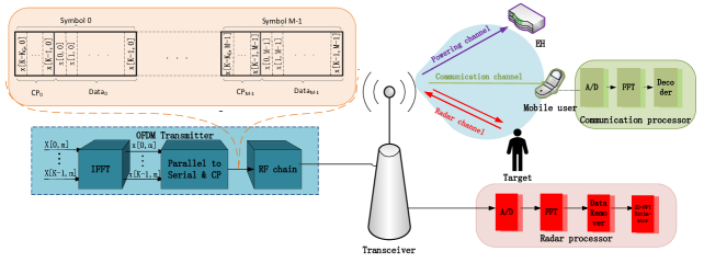
Figure 1: System and OFDM Signal Model for ISCAP.

II-A Transmit Signal

Without loss of generality, we consider a SISO ISCAP system as shown in Fig. 1, with a multi-functional transmitter and separated receivers for sensing, communications and powering, among which the sensing receiver is co-located with the transmitter. Besides the block model of the ISCAP system, Fig. 1 also depicts the OFDM symbol model at the transmitter, where $M$ OFDM symbols with $K$ orthogonal subcarriers and $K_{G}$ CP sub-pulses for each OFDM symbol are used.

The CS at the $k^{\text{th}}$ ($k=0,~{}\cdots,~{}K-1$) subcarrier of the $m^{\text{th}}$ ($m=0,~{}\cdots,~{}M-1$) OFDM symbol can be expressed as:

$$X[k,~{}m]\overset{\vartriangle}{=}{X}^{\mathrm{R}}[k,~{}m]+j{X}^{\mathrm{I}}[k,~{}m],$$ (1)

where ${X}^{\mathrm{R}}[k,~{}m]\sim\mathcal{N}({\mu}^{\mathrm{R}}_{k},~{}{{\sigma}^{\mathrm{R}}_{k}}^{2})$ and ${X}^{\mathrm{I}}[k,~{}m]\sim\mathcal{N}({\mu}^{\mathrm{I}}_{k},~{}{{\sigma}^{\mathrm{I}}_{k}}^{2})$ (assume the same input distribution spectrum across OFDM symbols). Hence, the average power on the real and imaginary part of the $k^{\mathrm{th}}$ subcarrier is given as:

$${p}^{\mathrm{R}}_{k}\overset{\vartriangle}{=} \mathbb{E}_{X^{\mathrm{R}}[k,~{}m]}\left\{{X^{\mathrm{R}}[k,~{}m]}^{2}\right\}={{\mu}^{\mathrm{R}}_{k}}^{2}+{{\sigma}^{\mathrm{R}}_{k}}^{2},~{}\forall~{}m,$$ (2a)

$${p}^{\mathrm{I}}_{k}\overset{\vartriangle}{=} \mathbb{E}_{X^{\mathrm{I}}[k,~{}m]}\left\{{X^{\mathrm{I}}[k,~{}m]}^{2}\right\}={{\mu}^{\mathrm{I}}_{k}}^{2}+{{\sigma}^{\mathrm{I}}_{k}}^{2},~{}\forall~{}m.$$ (2b)

After IDFT, we obtain the time domain signal $x[n,~{}m]$ ($n=0,~{}\cdots,~{}K-1$), namely the $n^{\text{th}}$ sub-pulse of the $m^{\text{th}}$ symbol, which, after adding the CP, becomes:

$$x_{\text{CP}}[n,~{}m]=x[\left<n-K_{G}\right>_{K},~{}m],~{}n=0,~{}\cdots,~{}K^{\prime}-1,$$ (3)

where $K^{\prime}=K_{G}+K$.

Then, the baseband signal is:

$$x(t)= \sum_{m=0}^{M-1}\sum_{n=0}^{K^{\prime}-1}x_{\text{CP}}[n,~{}m]\text{sinc}\left[Bt-(n+mK^{\prime})\right]$$ (4a)

$$\overset{\bigtriangleup}{=} \sum_{q=0}^{K^{\prime}M-1}x_{\text{CP}}[q]\text{sinc}\left[Bt-q\right],~{}(q=mK^{\prime}+n),$$ (4b)

with $x_{\text{CP}}[q]=x_{\text{CP}}[n,~{}m]$ and $B$ is the bandwidth of the OFDM signal.

After up-converting, we have the transmit signal as:

$$x_{\text{RF}}(t) =\sum_{m=0}^{M-1}\sum_{n=0}^{K^{\prime}-1}x_{\text{CP}}[n,~{}m]\text{sinc}\left[Bt-(n+mK^{\prime})\right]e^{j2\pi f_{c}t},$$ (5)

where $f_{c}$ is the central frequency.

For future analysis, we define the following vectors:

$$\mbox{Symbol mean vector:}~{}\boldsymbol{\mu}\overset{\vartriangle}{=} \left[{\mu}^{\mathrm{R}}_{0},~{}{\mu}^{\mathrm{R}}_{1},~{}\cdots,~{}{\mu}^{\mathrm{R}}_{K-1},~{}{\mu}^{\mathrm{I}}_{0},~{}\cdots,~{}{\mu}^{\mathrm{I}}_{K-1}\right]^{T},$$ (6a)

$$\mbox{Symbol variance vector:}~{}\boldsymbol{\sigma}\overset{\vartriangle}{=} \left[{{\sigma}^{\mathrm{R}}_{0}}^{2},~{}{{\sigma}^{\mathrm{R}}_{1}}^{2},~{}\cdots,~{}{{\sigma}^{\mathrm{R}}_{K-1}}^{2},~{}{{\sigma}^{\mathrm{I}}_{0}}^{2},~{}\cdots,~{}{{\sigma}^{\mathrm{I}}_{K-1}}^{2}\right]^{T},$$ (6b)

$$\text{Symbol power vector:}~{}\mathbf{p}\overset{\vartriangle}{=} \left[{p}^{\mathrm{R}}_{0},~{}{p}^{\mathrm{R}}_{1},~{}\cdots,~{}{p}^{\mathrm{R}}_{K-1},~{}{p}^{\mathrm{I}}_{0},~{}\cdots,~{}{p}^{\mathrm{I}}_{K-1}\right]^{T}$$ (6c)

$$\text{Symbol mean matrix:}~{}\mathbf{U}\overset{\vartriangle}{=} \boldsymbol{\mu}\boldsymbol{\mu}^{T}$$ (6d)

$$\text{Power allocation matrix:}~{}\mathbf{P}\overset{\vartriangle}{=} \mathbf{U}+\text{diag}\left(\boldsymbol{\sigma}\right),$$ (6e)

where $\mathbf{U}$ and $\mathbf{P}$ are defined for Section LABEL:sec_sim, where we will optimize w.r.t $\mathbf{U}$ and $\mathbf{P}$ to decide $\boldsymbol{\mu}$ and $\boldsymbol{\sigma}$.

II-B Metric for Powering

This section models the received signal at the EH, and derives the corresponding scaling term of the harvested power as the powering metric.

Assume that the signal is transmitted over a multipath channel with $L$ paths, where the gain and delay of the $l^{\text{th}}$ $(0\leq~{}l\leq~{}L-1)$ tap are respectively $a_{l}$ and $\tau_{l}$. The real received signal at EH is:

$$y_{\text{RF}}(t)= \sqrt{2}\mathfrak{R}\left\{\sum_{l=0}^{L-1}a_{l}x_{\text{RF}}(t-\tau_{l})+w(t)\right\},$$ (7)

where $w(t)\sim\mathcal{CN}(0,~{}\sigma_{\mathrm{n_{P}}}^{2})$ is the additive white Gaussian noise (AWGN) at EH.

At EH, the impinging signal $y_{\text{RF}}(t)$ is converted into direct current via a rectenna circuit for power harvesting. We model the non-linear rectenna referring to [clerckx2016waveform], which is composed of an ideal diode and a low pass filter. This rectenna has been modelled sufficiently in [clerckx2016waveform] with deterministic multi-sine signals, whose output harvested power is proved in proportion to a scaling term $z_{\mathrm{DC}}$. The scaling term $z_{\mathrm{DC}}$ is then extended in [varasteh2019swipt] to wideband OFDM signals with random CSs, as a function of CS input distribution, which is written as:

$$z_{\mathrm{DC}}= \mathbb{E}_{x}\left\{\mathcal{E}\left[k_{2}y_{\text{RF}}(t)^{2}+k_{4}y_{\text{RF}}(t)^{4}\right]\right\}$$ (8a)

$$= \sum_{m=0}^{M-1}\sum_{n=0}^{K^{\prime}-1}\frac{k_{2}}{M}\mathbb{E}_{x}\left\{|y[n,~{}m]|^{2}\right\}+$$

$$\sum_{m=0}^{M-1}\sum_{n=0}^{K^{\prime}-1}\frac{3k_{4}}{4M}\left(\mathbb{E}_{x}\left\{|y[n,~{}m]|^{4}\right\}+\mathbb{E}_{x}\left\{|\widetilde{y}[n,~{}m]|^{4}\right\}\right),$$ (8b)

where $k_{2}=0.024$ and $k_{4}=19.145$ [clerckx2016waveform]. In (8b), denote $y(t)$ as the complex baseband signal of $y_{\text{RF}}(t)$. Then, $y[n,~{}m]$ and $\widetilde{y}[n,~{}m]$ are the samples of $y(t)$ taken at times $t={(K^{\prime}m+n)}/{B}$ and ${(2K^{\prime}m+2n+1)}/{2B}$, which collectively form a sequence of samples capturing the power of $y(t)$ (based on the sampling theorem and Parseval’s theorem [34]). It is noteworthy that [varasteh2019swipt] does not account for the harvested power attributed by the CP part of OFDM signals when expressing (8b) as a function of the input distribution, which we address in the following.

If sampling at $t={(K^{\prime}m+n)}/{B}$, $y[n,~{}m]$ is given by:

$$y[n,~{}m]= y({(K^{\prime}m+n)}/{B})$$ (9a)

$$= \sum_{l}a_{l}\sum_{q}x_{\text{CP}}[q]\text{sinc}\left[{K^{\prime}m+n}-q-l\right]+w[n,~{}m]$$ (9b)

$$= \sum_{l}a_{l}x_{\text{CP}}[{K^{\prime}m+n}-l]+w[n,~{}m]$$ (9c)

$$= \sum_{l}a_{l}x_{\text{CP}}[n-l,~{}m]+w[n,~{}m],$$ (9d)

where $x_{\text{CP}}[n-l,~{}m]=x_{\text{CP}}[K^{\prime}+n-l,~{}m-1]$ for $n<l$. $w[n,~{}m]$ is the sampled noise at ${y}[n,~{}m]$.

Similarly, if sampling at $t=({2K^{\prime}m+2n+1})/{2B}$, $\widetilde{y}[n,~{}m]$ is given by:

$$\widetilde{y}[n,~{}m]= y(({2K^{\prime}m+2n+1})/{2B})$$ (10a)

$$= \sum_{l}a_{l}\sum_{q}x_{\text{CP}}[q]\text{sinc}\left[\frac{2K^{\prime}m+2n+1}{2}-q-\tau_{l}\right]+w[n,~{}m]$$ (10b)

$${=} \sum_{j}x_{\text{CP}}[K^{\prime}m+n-j]\sum_{l}a_{l}\text{sinc}\left[j+\frac{1}{2}-l\right]+w[n,~{}m]$$

$$~{}~{}({j=K^{\prime}m+n-q})$$ (10c)

$$\overset{\vartriangle}{=} \sum_{j}\widetilde{a}_{j}x_{\text{CP}}[n-j,~{}m]+\widetilde{w}[n,~{}m],$$ (10d)

$$\mbox{where}~{}\widetilde{a}_{j}= \begin{cases}\sum_{l}a_{l}\text{sinc}\left[j+\frac{1}{2}-l\right],&~{}0\leq j\leq L-1;\\ 0~{}(\text{approximate}),&~{}j>L,\end{cases}$$ (10e)

where $\widetilde{w}[n,~{}m]$ is the sampled noise at $\widetilde{y}[n,~{}m]$.

Remark 1.

$\widetilde{y}[n,~{}m]$ in (10d) is similar to ${y}[n,~{}m]$ in (9d), with $a_{l}$ substituted by $\widetilde{a}_{l}$. Hence, most of the future analysis related with ${y}[n,~{}m]$ can be adopted to $\widetilde{y}[n,~{}m]$ directly after changing the coefficient.

Given any $m$, the expression of ${y}[n,~{}m]$ in (9d) (or $\widetilde{y}[n,~{}m]$ in (10d)) are classified into two parts: (i) the CP duration for $0\leq n\leq K_{G}-1$ over which the received sub-pulses involves interaction between the $m^{\text{th}}$ OFDM symbol and the $(m-1)^{\text{th}}$ OFDM symbol; (ii) the data duration for $K_{G}\leq n\leq K^{\prime}-1$ where there is no inter-symbol interference. Hence, the final harvested power in (8b) also needs consideration from these two parts.

In the following, we first consider the sub-pulses’ power over the $m^{\text{th}}$ data duration ($K_{G}\leq n\leq K^{\prime}-1$) and then move to the sub-pulses’ power over the $m^{\text{th}}$ CP duration ($0\leq n\leq K_{G}-1$). For future analysis, we define the vector that collects the $m^{\text{th}}$ transmit OFDM symbol in the frequency domain as:

$$\mathbf{x}_{m}\overset{\vartriangle}{=} \left[X[0,~{}m],~{}\cdots,~{}X[K-1,~{}m]\right]^{T},~{}m=0,~{}\cdots,~{}M-1,$$ (11a)

$$\mathbf{\overline{x}}_{m}\overset{\vartriangle}{=} \left[\mathfrak{R}\{\mathbf{x}_{m}\}^{T},~{}\mathfrak{I}\{\mathbf{x}_{m}\}^{T}\right]^{T}.$$ (11b)

Furthermore, from (9d) and (10d), we define the complex gain of the frequency-domain powering channel as:

$$\mathbf{H}_{\mathrm{P}}\overset{\vartriangle}{=} \text{diag}\left([h_{\mathrm{P,~{}0}},~{}\cdots,~{}h_{\mathrm{P,~{}K-1}}]\right),~{}\mbox{with}~{}h_{\mathrm{P},~{}k}=\text{IDFT}\left\{a_{l}\right\}_{(k)};$$ (12a)

$$\widetilde{\mathbf{H}}_{\mathrm{P}}\overset{\vartriangle}{=} \text{diag}\left(\left[\widetilde{h}_{\mathrm{P,~{}0}},~{}\cdots,~{}\widetilde{h}_{\mathrm{P,~{}K-1}}\right]\right),~{}\mbox{with}~{}\widetilde{h}_{\mathrm{P},~{}k}=\text{IDFT}\left\{\widetilde{a}_{l}\right\}_{(k)}.$$ (12b)

II-B1 Power of data duration

Starting from the data duration ($K_{G}\leq n\leq K^{\prime}-1$), take $y[n,~{}m]$ as an example first. $y[n,~{}m]$ (for $K_{G}\leq n\leq K^{\prime}-1$) can be re-expressed as:

$$y[n,~{}m]= \text{IDFT}\left\{\mathbf{H}_{\mathrm{P}}\mathbf{x}_{m}\right\}_{(n)}+w[n,~{}m]$$ (13a)

$$= {\mathbf{a}^{\mathrm{R}}_{n}}^{T}\mathbf{\overline{x}}_{m}+j{\mathbf{a}^{\mathrm{I}}_{n}}^{T}\mathbf{\overline{x}}_{m}+w[n,~{}m],$$ (13b)

$$\mbox{with}~{}{\mathbf{a}^{\mathrm{R}}_{n}}= [\mathfrak{R}\left\{{\mathbf{f}_{n}\mathbf{H}_{\mathrm{P}}}\right\},~{}-\mathfrak{I}\left\{{\mathbf{f}_{n}\mathbf{H}_{\mathrm{P}}}\right\}]^{T},$$ (13c)

$${\mathbf{a}^{\mathrm{I}}_{n}}= [\mathfrak{I}\left\{{\mathbf{f}_{n}\mathbf{H}_{\mathrm{P}}}\right\},~{}\mathfrak{R}\left\{{\mathbf{f}_{n}\mathbf{H}_{\mathrm{P}}}\right\}]^{T},$$ (13d)

$$\mathbf{f}_{n}= \left[1,~{}e^{j\frac{2\pi n}{K}},~{}...,~{}e^{j\frac{2\pi n(K-1)}{K}}\right]$$

$$(\text{the }n^{\text{th}}\text{ row of the IDFT matrix}).$$ (13e)

Similarly, for $\widetilde{y}[n,~{}m]$, we have:

$$\widetilde{y}[n,~{}m]= \mbox{$\widetilde{\mathbf{a}}^{\mathrm{R}}_{n}$}^{T}\mathbf{\overline{x}}_{m}+j\mbox{$\widetilde{\mathbf{a}}^{\mathrm{I}}_{n}$}^{T}\mathbf{\overline{x}}_{m}+\widetilde{w}[n,~{}m],$$ (14a)

$$\mbox{with}~{}{\widetilde{\mathbf{a}}^{\mathrm{R}}_{n}}= \left[\mathfrak{R}\left\{{\mathbf{f}_{n}\widetilde{\mathbf{H}}_{\mathrm{P}}}\right\},~{}-\mathfrak{I}\left\{{\mathbf{f}_{n}\widetilde{\mathbf{H}}_{\mathrm{P}}}\right\}\right]^{T},$$ (14b)

$${\widetilde{\mathbf{a}}^{\mathrm{I}}_{n}}= \left[\mathfrak{I}\left\{{\mathbf{f}_{n}\widetilde{\mathbf{H}}_{\mathrm{P}}}\right\},~{}\mathfrak{R}\left\{{\mathbf{f}_{n}\widetilde{\mathbf{H}}_{\mathrm{P}}}\right\}\right]^{T}.$$ (14c)

On this basis, the second-order and the fourth-order expectations of $y[n,~{}m]$ in (8b), i.e., $\mathbb{E}\left\{|y[n,~{}m]|^{2}\right\}$ and $\mathbb{E}\left\{|y[n,~{}m]|^{4}\right\}$, are given in (15a) and (15) respectively (Details in Appendix LABEL:appen1). Following the same way, we also give the fourth-order expectations of $\widetilde{y}[n,~{}m]$, i.e., $\mathbb{E}\left\{|\widetilde{y}[n,~{}m]|^{4}\right\}$, in (15).

$$\mathbb{E}\left\{|y[n,~{}m]|^{2}\right\}= \mathrm{Tr}\left(\mathbf{A}_{n}\mathbf{P}\right)+\sigma_{\mathrm{n_{P}}}^{2}\overset{\vartriangle}{=}z^{\text{data},~{}2}_{\text{DC},~{}n}\left(\mathbf{P},~{}\mathbf{U}\right),$$ (15a)

$$\mathbb{E}\left\{|y[n,~{}m]|^{4}\right\}= \mathrm{Tr}^{2}\left(\mathbf{A}_{n}\mathbf{P}\right)+6\sigma_{\mathrm{n_{P}}}^{2}\mathrm{Tr}\left(\mathbf{A}_{n}\mathbf{P}\right)+2\mathrm{Tr}\left(\mathbf{A}_{n}\mathbf{P}\mathbf{A}_{n}\mathbf{P}\right)$$

$$-2\mathrm{Tr}\left(\mathbf{A}_{n}\mathbf{U}\mathbf{A}_{n}\mathbf{U}\right)+3\sigma_{\mathrm{n_{P}}}^{4}$$ (15b)

$$\overset{\vartriangle}{=} z^{\text{data},~{}4}_{\text{DC},~{}n}\left(\mathbf{P},~{}\mathbf{U}\right),$$ (15c)

$$\mathbb{E}\left\{|\widetilde{y}[n,~{}m]|^{4}\right\}= \mathrm{Tr}^{2}\left(\widetilde{\mathbf{A}}_{n}\mathbf{P}\right)+6\sigma_{\mathrm{n_{P}}}^{2}\mathrm{Tr}\left(\mathbf{A}_{n}\mathbf{P}\right)+2\mathrm{Tr}\left(\widetilde{\mathbf{A}}_{n}\mathbf{P}\widetilde{\mathbf{A}}_{n}\mathbf{P}\right)$$

$$-2\mathrm{Tr}\left(\widetilde{\mathbf{A}}_{n}\mathbf{U}\widetilde{\mathbf{A}}_{n}\mathbf{U}\right)+3\sigma_{\mathrm{n_{P}}}^{4}$$ (15d)

$$\overset{\vartriangle}{=} \widetilde{z}^{\text{data},~{}4}_{\text{DC},~{}n}\left(\mathbf{P},~{}\mathbf{U}\right),$$ (15e)

$$\mbox{with}~{}\mathbf{A}_{n}= {\mathbf{a}^{\mathrm{R}}_{n}}{\mathbf{a}^{\mathrm{R}}_{n}}^{T}+{\mathbf{a}^{\mathrm{I}}_{n}}{\mathbf{a}^{\mathrm{I}}_{n}}^{T},$$ (15f)

$$\widetilde{\mathbf{A}}_{n}= \mbox{$\widetilde{\mathbf{a}}^{\mathrm{R}}_{n}$}\mbox{$\widetilde{\mathbf{a}}^{\mathrm{R}}_{n}$}^{T}+\mbox{$\widetilde{\mathbf{a}}^{\mathrm{I}}_{n}$}\mbox{$\widetilde{\mathbf{a}}^{\mathrm{I}}_{n}$}^{T}.$$ (15g)

II-B2 Power of CP duration

Based on (9d), $y[n,~{}m]$ (for $0~{}\leq n~{}\leq K_{G}-1$) can be written as:

$$y[n,~{}m]= \sum^{n}_{l=0}a_{l}x_{\text{CP}}[n-l,~{}m]+\sum^{K_{G}-1}_{l=n+1}a_{l}x_{\text{CP}}[K^{\prime}+n-l,~{}m-1]$$

$$+w[n,~{}m]$$ (16a)

$$= \sum^{n}_{l=0}a_{l}x[K-K_{G}+n-l,~{}m]$$

$$+\sum^{K_{G}-1}_{l=n+1}a_{l}x[K+n-l,~{}m-1]+w[n,~{}m]$$ (16b)

$$= \sum^{K-K_{G}+n}_{p=K-K_{G}}a_{K-K_{G}+n-p}x[p,~{}m]$$

$$+\sum^{K-1}_{p=K-K_{G}+n+1}a_{K+n-p}x[p,~{}m-1]+w[n,~{}m]$$ (16c)

$$= {\mathbf{b}_{1,~{}n}}^{T}\mathbf{x}_{m}+{\mathbf{b}_{2,~{}n}}^{T}\mathbf{{x}}_{m-1}+w[n,~{}m],$$ (16d)

$$= \mbox{$\mathbf{b}^{\mathrm{R}}_{1,~{}n}$}^{T}\mathbf{\overline{x}}_{m}+\mbox{$\mathbf{b}^{\mathrm{R}}_{2,~{}n}$}^{T}\mathbf{\overline{x}}_{m-1}$$

$$+j\left(\mbox{$\mathbf{b}^{\mathrm{I}}_{1,~{}n}$}^{T}\mathbf{\overline{x}}_{m}+\mbox{$\mathbf{b}^{\mathrm{I}}_{2,~{}n}$}^{T}\mathbf{\overline{x}}_{m-1}\right)+w[n,~{}m],$$ (16e)

$$\mbox{with}~{}{\mathbf{b}_{i,~{}n}=} \text{DFT}{\left\{\mathbf{a}_{\mathrm{CP}i,~{}n}\right\},~{}\text{for }i=1,~{}2},$$ (16f)

$${a}_{\mathrm{CP}1,~{}n,~{}k}= \begin{cases}a_{K-K_{G}+n-k},~{}&K-K_{G}\leq k\leq K-K_{G}+n,\\ 0,~{}&\text{otherwise},\end{cases}$$ (16g)

$${a}_{\mathrm{CP}2,~{}n,~{}k}= \begin{cases}a_{K+n-k},~{}&K-K_{G}+n-1~{}\leq k~{}\leq K-1,\\ 0,~{}&\text{otherwise},\end{cases}$$ (16h)

$$\mbox{$\mathbf{b}^{\mathrm{R}}_{i,~{}n}$}= \left[\mathfrak{R}\left\{{\mathbf{b}_{i,~{}n}}^{T}\right\},~{}-\mathfrak{I}\left\{{\mathbf{b}_{i,~{}n}}^{T}\right\}\right]^{T},$$ (16i)

$$\mbox{$\mathbf{b}^{\mathrm{I}}_{i,~{}n}$}= \left[\mathfrak{I}\left\{{\mathbf{b}_{i,~{}n}}^{T}\right\},~{}\mathfrak{R}\left\{{\mathbf{b}_{i,~{}n}}^{T}\right\}\right]^{T}.$$ (16j)

Similarly, $\widetilde{y}[n,~{}m]$ ($0~{}\leq n~{}\leq K_{G}-1$) can be re-written as:

$$\widetilde{y}[n,~{}m]= \mbox{$\widetilde{\mathbf{b}}^{\mathrm{R}}_{1,~{}n}$}^{T}\mathbf{\overline{x}}_{m}+\mbox{$\widetilde{\mathbf{b}}^{\mathrm{R}}_{2,~{}n}$}^{T}\mathbf{\overline{x}}_{m-1}+j\left(\mbox{$\widetilde{\mathbf{b}}^{\mathrm{I}}_{1,~{}n}$}^{T}\mathbf{\overline{x}}_{m}+\mbox{$\widetilde{\mathbf{b}}^{\mathrm{I}}_{2,~{}n}$}^{T}\mathbf{\overline{x}}_{m-1}\right)$$

$$+\widetilde{w}[n,~{}m],$$ (17)

where the corresponding expressions for ${\widetilde{\mathbf{b}}^{\mathrm{R}}_{i,~{}n}}$ and $\widetilde{\mathbf{b}}^{\mathrm{I}}_{i,~{}n}$ $(i=1,~{}2)$ are obtained by replacing $a_{l}$ with $\widetilde{a}_{l}$ respectively in (16f)-(16j).

Consequently, the second-order and the fourth-order expectations of the CP duration sub-pulses are (Details in Appendix LABEL:appen2):

$$\mathbb{E}\left\{|y[n,~{}m]|^{2}\right\}= \mathrm{Tr}\left(\mathbf{B}_{n}\mathbf{P}+2\mathbf{D}_{n}\mathbf{U}\right)+\sigma_{\mathrm{n_{P}}}^{2}\overset{\vartriangle}{=}z^{\text{CP},~{}2}_{\text{DC},~{}n}\left(\mathbf{P},~{}\mathbf{U}\right),$$ (18a)

$$\mathbb{E}\left\{|y[n,~{}m]|^{4}\right\}= \mathrm{Tr}^{2}\left({\mathbf{B}}_{n}\mathbf{P}+2\mathbf{D}_{n}\mathbf{U}\right)+6\sigma_{\mathrm{n_{P}}}^{2}\mathrm{Tr}\left(\mathbf{B}_{n}\mathbf{P}+2\mathbf{D}_{n}\mathbf{U}\right)$$

$$+2\mathrm{Tr}\left(\mathbf{B}_{1,~{}n}\mathbf{P}\mathbf{B}_{1,~{}n}\mathbf{P}+\mathbf{B}_{2,~{}n}\mathbf{P}\mathbf{B}_{2,~{}n}\mathbf{P}\right)$$

$$+4\mathrm{Tr}\left(\mathbf{D}_{n}\mathbf{P}\mathbf{D}_{n}^{T}\mathbf{P}+\mathbf{D}_{n}\mathbf{U}\mathbf{D}_{n}\mathbf{U}+\mathbf{B}_{1,~{}n}\mathbf{U}\mathbf{B}_{2,~{}n}\mathbf{U}\right)$$

$$+4\mathrm{Tr}\left(\mathbf{B}_{1,~{}n}\mathbf{P}\mathbf{D}_{n}\mathbf{U}+\mathbf{B}_{2,~{}n}\mathbf{P}\mathbf{D}^{T}_{n}\mathbf{U}+\mathbf{B}_{1,~{}n}\mathbf{U}\mathbf{D}^{T}_{n}\mathbf{P}\right)$$

$$+4\mathrm{Tr}\left(\mathbf{B}_{2,~{}n}\mathbf{U}\mathbf{D}_{n}\mathbf{P}\right)-2\mathrm{Tr}\left(\mathbf{E}_{n}\mathbf{U}\mathbf{E}_{n}^{T}\mathbf{U}\right)+3\sigma_{\mathrm{n_{P}}}^{4}$$

$$\overset{\vartriangle}{=} z^{\text{CP},~{}4}_{\text{DC},~{}n}\left(\mathbf{P},~{}\mathbf{U}\right),$$ (18b)

$$\mathbb{E}\left\{|\widetilde{y}[n,~{}m]|^{4}\right\}= \mathrm{Tr}^{2}\left(\widetilde{\mathbf{B}}_{n}\mathbf{P}+2\widetilde{\mathbf{D}}_{n}\mathbf{U}\right)+6\sigma_{\mathrm{n_{P}}}^{2}\mathrm{Tr}\left(\widetilde{\mathbf{B}}_{n}\mathbf{P}+2\widetilde{\mathbf{D}}_{n}\mathbf{U}\right)$$

$$+2\mathrm{Tr}\left(\widetilde{\mathbf{B}}_{1,~{}n}\mathbf{P}\widetilde{\mathbf{B}}_{1,~{}n}\mathbf{P}+\widetilde{\mathbf{B}}_{2,~{}n}\mathbf{P}\widetilde{\mathbf{B}}_{2,~{}n}\mathbf{P}\right)$$

$$+4\mathrm{Tr}\left(\widetilde{\mathbf{D}}_{n}\mathbf{P}\widetilde{\mathbf{D}}_{n}^{T}\mathbf{P}+\widetilde{\mathbf{D}}_{n}\mathbf{U}\widetilde{\mathbf{D}}_{n}\mathbf{U}+\widetilde{\mathbf{B}}_{1,~{}n}\mathbf{U}\widetilde{\mathbf{B}}_{2,~{}n}\mathbf{U}\right)$$

$$+4\mathrm{Tr}\left(\widetilde{\mathbf{B}}_{1,~{}n}\mathbf{P}\widetilde{\mathbf{D}}_{n}\mathbf{U}+\widetilde{\mathbf{B}}_{2,~{}n}\mathbf{P}\widetilde{\mathbf{D}}^{T}_{n}\mathbf{U}\right)$$

$$+4\mathrm{Tr}\left(\widetilde{\mathbf{B}}_{1,~{}n}\mathbf{U}\widetilde{\mathbf{D}}^{T}_{n}\mathbf{P}+\widetilde{\mathbf{B}}_{2,~{}n}\mathbf{U}\widetilde{\mathbf{D}}_{n}\mathbf{P}\right)$$

$$-2\mathrm{Tr}\left(\widetilde{\mathbf{E}}_{n}\mathbf{U}\widetilde{\mathbf{E}}_{n}^{T}\mathbf{U}\right)+3\sigma_{\mathrm{n_{P}}}^{4}$$

$$\overset{\vartriangle}{=} \widetilde{z}^{\text{CP},~{}4}_{\text{DC},~{}n}\left(\mathbf{P},~{}\mathbf{U}\right),$$ (18c)

$$\mbox{with}~{}\mathbf{B}_{n}= \mathbf{B}_{1,~{}n}+\mathbf{B}_{2,~{}n},~{}\widetilde{\mathbf{B}}_{n}=\widetilde{\mathbf{B}}_{1,~{}n}+\widetilde{\mathbf{B}}_{2,~{}n},$$ (18d)

$${\mathbf{B}_{i,~{}n}=} {\mbox{$\mathbf{b}^{\mathrm{R}}_{i,~{}n}$}\mbox{$\mathbf{b}^{\mathrm{R}}_{i,~{}n}$}^{T}+\mbox{$\mathbf{b}^{\mathrm{I}}_{i,~{}n}$}\mbox{$\mathbf{b}^{\mathrm{I}}_{i,~{}n}$}^{T},~{}\text{for }i=1,~{}2,}$$ (18e)

$${\widetilde{\mathbf{B}}_{i,~{}n}=} {\mbox{$\widetilde{\mathbf{b}}^{\mathrm{R}}_{i,~{}n}$}\mbox{$\widetilde{\mathbf{b}}^{\mathrm{R}}_{i,~{}n}$}^{T}+\mbox{$\widetilde{\mathbf{b}}^{\mathrm{I}}_{i,~{}n}$}\mbox{$\widetilde{\mathbf{b}}^{\mathrm{I}}_{i,~{}n}$}^{T},~{}\text{for }i=1,~{}2,}$$ (18f)

$$\mathbf{D}_{n}= \mbox{$\mathbf{b}^{\mathrm{R}}_{1,~{}n}$}\mbox{$\mathbf{b}^{\mathrm{R}}_{2,~{}n}$}^{T}+\mbox{$\mathbf{b}^{\mathrm{I}}_{1,~{}n}$}\mbox{$\mathbf{b}^{\mathrm{I}}_{2,~{}n}$}^{T},$$ (18g)

$$\widetilde{\mathbf{D}}_{n}= \mbox{$\widetilde{\mathbf{b}}^{\mathrm{R}}_{1,~{}n}$}\mbox{$\widetilde{\mathbf{b}}^{\mathrm{R}}_{2,~{}n}$}^{T}+\mbox{$\widetilde{\mathbf{b}}^{\mathrm{I}}_{1,~{}n}$}\mbox{$\widetilde{\mathbf{b}}^{\mathrm{I}}_{2,~{}n}$}^{T}$$ (18h)

$$\mathbf{E}_{n}= {\mathbf{B}}_{1,~{}n}+\mathbf{D}_{n}+\mathbf{B}_{2,~{}n}^{T}+\mathbf{D}_{n}^{T},$$ (18i)

$$\widetilde{\mathbf{E}}_{n}= \widetilde{\mathbf{B}}_{1,~{}n}+\widetilde{\mathbf{D}}_{n}+\widetilde{\mathbf{B}}_{2,~{}n}^{T}+\widetilde{\mathbf{D}}_{n}^{T}.$$ (18j)

II-B3 Total power

After re-organization, the scaling term of the generated power of the $m^{\text{th}}$ OFDM symbol as a function of the input distribution is given as:

$$z_{\text{DC}}\left(\mathbf{P},~{}\mathbf{U}\right)$$

$$= \sum_{n=0}^{K_{G}-1}k_{2}z^{\text{CP},~{}2}_{\text{DC},~{}n}\left(\mathbf{P},~{}\mathbf{U}\right)+\frac{3k_{4}}{4}\left(z^{\text{CP},~{}4}_{\text{DC},~{}n}\left(\mathbf{P},~{}\mathbf{U}\right)+\widetilde{z}^{\text{CP},~{}4}_{\text{DC},~{}n}\left(\mathbf{P},~{}\mathbf{U}\right)\right)$$

$$+\sum_{n=K_{G}}^{K^{\prime}-1}k_{2}z^{\text{data},~{}2}_{\text{DC},~{}n}\left(\mathbf{P},~{}\mathbf{U}\right)+\frac{3k_{4}}{4}\left(z^{\text{data},~{}4}_{\text{DC},~{}n}\left(\mathbf{P},~{}\mathbf{U}\right)+\widetilde{z}^{\text{data},~{}4}_{\text{DC},~{}n}\left(\mathbf{P},~{}\mathbf{U}\right)\right).$$ (19)

II-C Metric for Sensing

In terms of sensing, we consider a point-target sensing scenario aiming at the range-velocity bin estimation. The sensing’s performance is guaranteed by restricting its aISPLD in terms of the ambiguity property. Indeed, according to [2022ISAC], the aISPLD is shown to be in proportion to the upper bound of the average FAP, i.e., the probability of incorrectly estimating the target’s range-velocity bin using the maximum likelihood estimator in OFDM ISAC systems in low SNR. On this basis, we express our sensing metric, $\overline{\text{UB}}_{\text{FAP}}$, as:

$$\overline{\text{UB}}_{\text{FAP}}(\mathbf{p},~{}\boldsymbol{\mu})= -M(K_{G}M-1)\mathbf{1}^{T}\mathbf{{p}}+{\sum_{(r,~{}v)\neq(0,~{}0)}\sqrt{g_{r,v}(\mathbf{{p}})+g_{2}(\boldsymbol{\mu})}},$$ (20a)

$$\mbox{with}~{}g_{r,v}(\mathbf{{p}})= M^{2}\delta\left(v\right)|\left(\mathbf{1}_{2}^{T}\otimes\mathbf{f}_{n}\right)\mathbf{{p}}|^{2}+2M\|\mathbf{{p}}\|^{2},$$ (20b)

$$g_{2}(\boldsymbol{\mu})= -2M\sum_{k=0}^{2K-1}|{\mu}_{k}|^{4},$$ (20c)

where $(r,~{}v)$ represents the range-velocity bin candidate for the OFDM ISAC system, with $r=0,~{}\cdots,~{}K_{G}-1$ and $v=-M/2,~{}\cdots,~{}M/2-1$. Assuming a target at $(r,~{}v)=(0,~{}0)$, the first sum term in (20a) represents the average peak lobe at $(r,~{}v)=(0,~{}0)$ and the second sum term in (20a) represents the upper bound of the average sum of side lobes where $(r,~{}v)\neq(0,~{}0)$.

Remark 2.

Given a transmit power constraint, i.e., a fixed $\mathbf{1}^{T}\mathbf{{p}}$, the aISPLD metric in (20) is minimized by maximizing the symbol mean at each subcarrier, i.e., $\boldsymbol{\mu}=\mathbf{p}$, while the optimal $\mathbf{p}$ is to be uniform across sub-carriers from [2022ISAC]. Intuitively, sensing prefers deterministic components that are represented by the symbol mean of the input distribution, in contrast with communications. In other words, the randomness of the CS magnitudes makes $\mathbf{p}$ random and hence degrades sensing.

Similar to the powering metric expression in (II-B3), we re-formulate the sensing metric $\overline{\text{UB}}_{\text{FAP}}(\mathbf{p},~{}\boldsymbol{\mu})$ in (20) as a function of $\mathbf{P}$ and $\mathbf{U}$:

$$\widetilde{\text{UB}}_{\text{FAP}}(\mathbf{P},~{}\mathbf{U})= -M(K_{G}M-1)\mathrm{Tr}\left(\mathbf{P}\right)$$

$$+{\sum_{(r,~{}v)\neq(0,~{}0)}\sqrt{\widetilde{g}_{r,v}\left(\mathbf{P}\right)+\widetilde{g}_{2}\left(\mathbf{U}\right)}},$$ (21a)

$$\mbox{with}~{}\widetilde{g}_{r,v}\left(\mathbf{P}\right)= \left({\mathbf{f}^{\mathrm{R}}_{r,v}}\text{diag}\left(\mathbf{P}\right)\right)^{2}+\left({\mathbf{f}^{\mathrm{I}}_{r,v}}\text{diag}\left(\mathbf{P}\right)\right)^{2}+2M\|\text{diag}\left(\mathbf{P}\right)\|^{2},$$ (21b)

$$\widetilde{g}_{2}(\mathbf{U})= -2M\|\text{diag}\left(\mathbf{U}\right)\|^{2},$$ (21c)

$$\mathbf{f}^{\mathrm{R/I}}_{r,v}= M\delta\left(v\right)\mathfrak{R/I}\left\{\mathbf{1}_{2}^{T}\otimes\mathbf{f}_{n}\right\}.$$ (21d)

II-D Metric for Communication

For the communication system, the complex received signal at the $k^{\text{th}}$ subcarrier is:

$$Y_{\mathrm{C}}[k,~{}m]= h_{\mathrm{C},~{}k}X[k,~{}m]+w_{\mathrm{C}}[k,~{}m],$$ (22)

where $h_{\mathrm{C},~{}k}$ is the complex gain of the communication channel of the $k^{\text{th}}$ subcarrier. $w_{\mathrm{C}}[k,~{}m]$ is the AWGN at the communication receiver with its noise power spectrum density being $\sigma_{\mathrm{n_{C}}}^{2}$.

Given that the variance of the real and imaginary part of $X[k,~{}m]$ are ${\sigma^{\mathrm{R}}_{k}}^{2}$ and ${\sigma^{\mathrm{I}}_{k}}^{2}$ respectively, the average communication achievable rate in OFDM can be written as[varasteh2019swipt]:

$$R\left(\left\{\sigma^{\mathrm{R}}_{k},~{}\sigma^{\mathrm{I}}_{k}\right\}\right)= \frac{1}{2KM}\sum_{k,~{}m}\log~{}\left(1+{2K|h_{\mathrm{C},~{}k}|^{2}}{\sigma^{\mathrm{R}}_{k}}^{2}/(B\sigma^{2}_{\mathrm{n_{C}}})\right)$$

$$+\frac{1}{2KM}\sum_{k,~{}m}\log~{}\left(1+{2K|h_{\mathrm{C},~{}k}|^{2}}{\sigma^{\mathrm{I}}_{k}}^{2}/(B\sigma^{2}_{\mathrm{n_{C}}})\right).$$ (23)

(II-D) can be re-formulated in the vector form as:

$$R(\boldsymbol{\sigma})= \frac{1}{2K}\log~{}\det\left[\mathbf{I}_{2K}+\mathbf{C}_{1}\mathrm{diag}(\boldsymbol{\sigma})\right],$$ (24a)

$$\mbox{with}~{}\mathbf{C}_{1}= \text{diag}\left({\left[\mathbf{c}_{1}^{T},~{}\mathbf{c}_{1}^{T}\right]^{T}}\right),$$ (24b)

$${c}_{1,~{}k}= {2K|h_{\mathrm{C},~{}k}|^{2}}/(B\sigma^{2}_{\mathrm{n_{C}}}).$$ (24c)

III Optimal OFDM Waveform Design

In this section, we formulate the problem to optimize the performance region of the ISCAP system, i.e., to maximize the harvested power per symbol given constraints on the transmit power, the achievable rate (communication) and the aISPLD (sensing). Upon formulating the problem which is non-convex, we propose an ADMM-based algorithm to obtain a local optimal solution.

III-A Problem formulation

The optimization problem that maximizes the harvested power per symbol given achievable rate constraint and the aISPLD constraint is formulated as: P, U, σz_DC(P, U) in (II-B3), Tr(P)≤P_max R(σ) ≥C_min ~UB_FAP(P, U) ≤S_max U≥0 rank(U)= 1 σ⪰0 P=U+diag(σ), where $P_{\max}$ in (III-A) is the transmit power constraint at the transmitter, $C_{\min}$ in (III-A) is the minimum rate constraint for communication, and $S_{\max}$ in (III-A) is the maximal aISPLD constraint for sensing. Constraint (III-A) and (III-A) ensure a solution for $\mathbf{U}=\boldsymbol{\mu}\boldsymbol{\mu}^{T}$. (III-A) ensures positive covariance and (III-A) establishes the relationship between the variables as defined in (6d)-(6e).

III-B Problem optimization

The rank 1 constraint in problem (III-A) is relaxed first during the optimization and is handled at the final stage by Gaussian randomization [luo2010semidefinite]. On this basis, we solve the remaining optimization problem following an ADMM structure.

The ADMM structure of problem (III-A), relaxing the rank $1$ constraint in (III-A) is expressed as: P, U, σ -z_DC(P, U) +f_I, P,U(P, U)+f_I, σ, U(σ, U), U+diag(σ)-P=0, where $f_{\mathrm{I},~{}\mathbf{P},~{}\mathbf{U}}\left(\mathbf{P},~{}\mathbf{U}\right)$ is the indicator function of $\mathbf{P}$ and $\mathbf{U}$ corresponding to the constraint in (III-A) and (III-A), and $f_{\mathrm{I},~{}\boldsymbol{\sigma},~{}\mathbf{U}}\left(\boldsymbol{\sigma},~{}\mathbf{U}\right)$ is the indicator function of $\boldsymbol{\sigma}$ and $\mathbf{U}$ corresponding to the constraints in (III-A), (III-A), (III-A) and (III-A), i.e.,

$$f_{\mathrm{I},~{}\mathbf{P},~{}\mathbf{U}}\left(\mathbf{P},~{}\mathbf{U}\right):= f_{\mathrm{I}}\left(\mathrm{Tr}\left({\mathbf{P}}\right)\leq P_{\max}\right)+f_{\mathrm{I}}\left(\widetilde{\text{UB}}_{\text{FAP}}(\mathbf{P},~{}\mathbf{U})\leq S_{\max}\right),$$ (25)

$$f_{\mathrm{I},~{}\boldsymbol{\sigma},~{}\mathbf{U}}\left(\boldsymbol{\sigma},~{}\mathbf{U}\right):= f_{\mathrm{I}}\left(R(\boldsymbol{\sigma})\geq C_{\min}\right)+f_{\mathrm{I}}\left(\widetilde{\text{UB}}_{\text{FAP}}(\mathbf{P},~{}\mathbf{U})\leq S_{\max}\right)$$

$$+f_{\mathrm{I}}\left(\mathbf{U}\geq 0\right)+f_{\mathrm{I}}\left(\boldsymbol{\sigma}\succeq 0\right).$$ (26)

Following the ADMM structure in problem (III-B), the variables of $\mathbf{P}$, $\mathbf{U}$ and $\boldsymbol{\sigma}$ at the $l^{\text{th}}$ ADMM iteration are successively updated as in (27a)-(27c), where $\mathbf{V}^{(l)}$ is the alternating direction at the $l^{\text{th}}$ iteration and $\rho$ is the updating step-size in ADMM.

$$\scriptstyle\mathbf{P}^{(l+1)}\scriptstyle:= \scriptstyle\arg\min\left\{{-z_{\mathrm{DC}}\left(\mathbf{P},~{}{\mathbf{U}}^{(l)}\right)+f_{\mathrm{I},~{}\mathbf{P},\mathbf{U}}\left(\mathbf{P},\mathbf{U}^{(l)}\right)+}{\frac{\rho}{2}\|{\mathbf{U}}^{(l)}-\mathbf{P}+\text{diag}\left({\boldsymbol{\sigma}}^{(l)}\right)-{\mathbf{V}}^{(l)}\|^{2}}\right\},$$ (27a)

$$\scriptstyle{\left\{{\mathbf{U}}^{(l+1)},~{}{\boldsymbol{\sigma}}^{(l+1)}\right\}}:= \scriptstyle\arg\min\left\{{-z_{\mathrm{DC}}\left({\mathbf{P}}^{(l+1)},~{}\mathbf{U}\right)+f_{\mathrm{I},~{}\boldsymbol{\sigma},~{}\mathbf{U}}(\boldsymbol{\sigma},~{}\mathbf{U})+}{\frac{\rho}{2}\|-{\mathbf{P}}^{(l+1)}+\mathbf{U}+\text{diag}\left({\boldsymbol{\sigma}}\right)-{\mathbf{V}}^{(l)}\|^{2}}\right\},$$ (27b)

$$\scriptstyle{{\mathbf{V}}^{(l+1)}:=} \scriptstyle{{\mathbf{V}}^{(l)}+{\mathbf{P}}^{(l+1)}-{\mathbf{U}}^{(l+1)}-\text{diag}\left({\boldsymbol{\sigma}}^{(l+1)}\right)},$$ (27c)

 

Next, we solve the sub-problems in (27a) and (27b) respectively to update the variables $\mathbf{P}$, $\mathbf{U}$ and $\boldsymbol{\sigma}$.

III-B1 Updating ${\mathbf{P}}^{(l+1)}$

The sub-problem to solve (27a) is: P-z_DC(P, U^(l))+ρ2∥-P+U^(l)+diag(σ^(l))-V^(l)∥^2 Tr(P)≤P_max ~UB_FAP(P, U^(l)) ≤S_max, which is non-convex due to the objective $-z_{\mathrm{DC}}\left(\mathbf{P},~{}{\mathbf{U}}^{(l)}\right)$ and the constraint (III-B1). However, $-z_{\mathrm{DC}}\left(\mathbf{P},~{}{\mathbf{U}}^{(l)}\right)$ in the objective function is concave with respect to $\mathbf{P}$, and can be handled by using SCA. In SCA, the concave part of the objective function is successively substituted by a linear Taylor approximation operating at the point which is the local optimal of the previous round. Specifically, suppose $\mathbf{P}^{(t)}$ is the optimal point at the $t^{\text{th}}$ SCA iteration, then, at the $(t+1)^{\text{th}}$ iteration, $-z_{\mathrm{DC}}(\mathbf{P},{\mathbf{U}}^{(l)})$ in the objective function is substituted by:

$${z_{\mathrm{DC}}}^{(t+1)}\left(\mathbf{P},~{}{\mathbf{U}}^{(l)}\right)={z_{\mathrm{DC},~{}0}}^{(t)}\left(\mathbf{P}^{(t)},~{}{\mathbf{U}}^{(l)}\right)+\mathrm{Tr}\left({\mathbf{G}^{(t)}}^{T}\mathbf{P}\right),$$ (28)

where ${\mathbf{G}^{(t)}}$ is the first-order Taylor coefficient, expressed in (29). ${z_{\mathrm{DC},~{}0}}^{(t)}\left(\mathbf{P}^{(t)},~{}{\mathbf{U}}^{(l)}\right)$ is the Taylor constant to be omitted.

$$\scriptstyle{{\mathbf{G}^{(t)}}}= \scriptstyle{\sum_{n=K_{G}}^{K^{\prime}-1}k_{2}\mathbf{A}_{n}^{T}+\frac{3k_{4}}{4}\left[2\mathrm{Tr}\left(\mathbf{A}_{n}\mathbf{P}^{(t)}\right)\mathbf{A}_{n}^{T}+6\sigma_{\mathrm{n_{P}}}^{2}\mathbf{A}_{n}^{T}+4\mathbf{A}_{n}\mathbf{P}^{(t)}\mathbf{A}_{n}+2\mathrm{Tr}\left(\widetilde{\mathbf{A}}_{n}\mathbf{P}^{(t)}\right)\widetilde{\mathbf{A}}_{n}^{T}+6\sigma_{\mathrm{n_{P}}}^{2}\widetilde{\mathbf{A}}_{n}^{T}+4\widetilde{\mathbf{A}}_{n}\mathbf{P}^{(t)}\widetilde{\mathbf{A}}_{n}\right]}$$

$$\scriptstyle{+\sum_{n=0}^{K_{G}-1}k_{2}\mathbf{B}_{n}^{T}+\frac{3k_{4}}{4}\left[2\mathrm{Tr}\left(\mathbf{B}_{n}\mathbf{P}^{(t)}+2\mathbf{D}_{n}\mathbf{U}^{(l)}\right)\mathbf{B}_{n}^{T}+6\sigma_{\mathrm{n_{P}}}^{2}\mathbf{B}^{T}_{n}+2\mathrm{Tr}\left(\widetilde{\mathbf{B}}_{n}\mathbf{P}^{(t)}+2\widetilde{\mathbf{D}}_{n}\mathbf{U}^{(l)}\right)\widetilde{\mathbf{B}}_{n}^{T}+6\sigma_{\mathrm{n_{P}}}^{2}\widetilde{\mathbf{B}}^{T}_{n}\right]}$$

$$\scriptstyle{+\sum_{n=0}^{K_{G}-1}{3k_{4}}\left[\mathbf{B}_{1,~{}n}\left(\mathbf{P}^{(t)}\mathbf{B}_{1,~{}n}+\mathbf{U}^{(l)}\mathbf{D}_{n}^{T}\right)+\mathbf{D}^{T}_{n}\left(\mathbf{P}^{(t)}\mathbf{D}_{n}+\mathbf{U}^{(l)}\mathbf{B}_{2,~{}n}\right)+\mathbf{D}_{n}\left(\mathbf{P}^{(t)}\mathbf{D}_{n}^{T}+\mathbf{U}^{(l)}\mathbf{B}_{1,~{}n}\right)+\mathbf{B}_{2,~{}n}\left(\mathbf{P}^{(t)}\mathbf{B}_{2,~{}n}+\mathbf{U}^{(l)}\mathbf{D}_{n}\right)\right]}$$

$$\scriptstyle{+\sum_{n=0}^{K_{G}-1}{3k_{4}}\left[\widetilde{\mathbf{B}}_{1,~{}n}\left(\mathbf{P}^{(t)}\widetilde{\mathbf{B}}_{1,~{}n}+\mathbf{U}^{(l)}\widetilde{\mathbf{D}}_{n}^{T}\right)+\widetilde{\mathbf{D}}^{T}_{n}\left(\mathbf{P}^{(t)}\widetilde{\mathbf{D}}_{n}+\mathbf{U}^{(l)}\widetilde{\mathbf{B}}_{2,~{}n}\right)+\widetilde{\mathbf{D}}_{n}\left(\mathbf{P}^{(t)}\widetilde{\mathbf{D}}_{n}^{T}+\mathbf{U}^{(l)}\widetilde{\mathbf{B}}_{1,~{}n}\right)+\widetilde{\mathbf{B}}_{2,~{}n}\left(\mathbf{P}^{(t)}\widetilde{\mathbf{B}}_{2,~{}n}+\mathbf{U}^{(l)}\widetilde{\mathbf{D}}_{n}\right)\right]}.$$ (29)

 

Similarly, the non-linear constraint in (III-B1) is also approximated by its linear upper bound in each iteration of SCA. Since the concavity of (III-B1) comes from the square root function, we also approximate the square root function by using Taylor expansion:

$$\widetilde{\text{UB}}_{\text{FAP}}\left(\mathbf{P},~{}{\mathbf{U}}^{(l)}\right)$$

$$\leq -M(K_{G}M-1)\mathrm{Tr}\left(\mathbf{P}\right)+\sum_{(r,~{}v)\neq(0,~{}0)}\frac{2\left(\widetilde{g}_{r,v}\left({\mathbf{P}}^{(t)}\right)+\widetilde{g}_{2}\left({\mathbf{U}}^{(l)}\right)\right)}{\alpha^{(l,t)}_{r,v}}+$$

$$\sum_{(r,~{}v)\neq(0,~{}0)}\frac{\left[\widetilde{g}_{r,v}\left({\mathbf{P}}\right)+\widetilde{g}_{2}\left(\mathbf{U}^{(l)}\right)-\widetilde{g}_{r,v}\left({\mathbf{P}^{(t)}}\right)-\widetilde{g}_{2}\left(\mathbf{U}^{(l)}\right)\right]}{\alpha^{(l,t)}_{r,v}}$$ (30a)

$$= \alpha^{(l,t)}-M(K_{G}M-1)\mathrm{Tr}\left(\mathbf{P}\right)+\sum_{(r,~{}v)\neq(0,~{}0)}\frac{\widetilde{g}_{r,v}\left(\mathbf{P}\right)}{\alpha^{(l,t)}_{r,v}}$$ (30b)

$$\overset{\bigtriangleup}{=} \widetilde{\text{UB}}^{(t)}_{\text{FAP}}\left(\mathbf{P}\right),$$ (30c)

with

$$\alpha^{(l,t)}_{r,v}= 2\sqrt{\widetilde{g}_{r,v}\left(\mathbf{P}^{(t)}\right)+\widetilde{g}_{2}\left(\mathbf{U}^{(l)}\right)},$$ (31a)

$$\alpha^{(l,t)}= \sum_{(r,~{}v)\neq(0,~{}0)}\frac{\widetilde{g}_{r,v}\left(\mathbf{P}^{(t)}\right)+2\widetilde{g}_{2}\left(\mathbf{U}^{(l)}\right)}{\alpha^{(l,t)}_{r,v}}.$$ (31b)

Hence, combing (28) and (30), the sub-problem to solve problem (III-B1) becomes: P-Tr(G^(t)^TP)+ρ2∥P-U^(l)-diag(σ^(l))+V^(l)∥^2, Tr(P) ≤P_max ~UB^(t)_FAP(P) ≤S_max, which is a convex Quadratic Constrained Quadratic Programming (QCQP) problem, whose Lagrangian is given by:

$$L(\mathbf{P},~{}u_{1},~{}u_{2})= -\sum_{n}\mathrm{Tr}\left({\mathbf{G}^{(t)}}^{T}\mathbf{P}\right)+\frac{\rho}{2}\|\mathbf{P}-\mathbf{U}^{(l)}-\text{diag}\left({\boldsymbol{\sigma}}^{(l)}\right)+\mathbf{V}^{(l)}\|^{2}$$

$$+u_{1}\left(\mathrm{Tr}\left(\mathbf{P}\right)-P_{\max}\right)+u_{2}\left(\widetilde{\text{UB}}^{(t)}_{\text{FAP}}(\mathbf{P})-S_{\max}\right),$$ (32)

where $u_{1}$ and $u_{2}$ are the non-negative Lagrange multipliers.

Taking the first-order derivative and combining (30c), we have:

$$\frac{\partial L(\mathbf{P},~{}u_{1},~{}u_{2})}{\partial\mathbf{P}}$$

$$= -\mathbf{G}^{(t)}+\rho\left(\mathbf{P}-\mathbf{U}^{(l)}-\text{diag}\left(\boldsymbol{\sigma}^{(l)}\right)+\mathbf{V}^{(l)}\right)+\left[{u_{1}}-u_{2}M(K_{G}M-1)\right]\mathbf{I}_{2K}$$

$$+u_{2}\text{diag}\left\{\sum_{\footnotesize{(r,~{}v)\neq(0,~{}0)}}\left[\frac{2{\mathbf{F}}^{\mathrm{R}}_{r,v}+2{\mathbf{F}}^{\mathrm{I}}_{r,v}+4M\mathbf{I}_{2K}}{\alpha^{(l,t)}_{r,v}}\right]\text{diag}\left(\mathbf{P}\right)\right\},$$ (33)

where ${\mathbf{F}}^{\mathrm{R}}_{r,v}={\mathbf{f}^{\mathrm{R}}_{r,v}}^{T}{\mathbf{f}^{\mathrm{R}}_{r,v}}$ and ${\mathbf{F}}^{\mathrm{I}}_{r,v}={\mathbf{f}^{\mathrm{I}}_{r,v}}^{T}{\mathbf{f}^{\mathrm{I}}_{r,v}}$.

Equating (33) to $\mathbf{0}$, we observe that, for the non-diagonal elements of $\mathbf{P}$, the stationary point is irrelevant with the multipliers $u_{1}$ and $u_{2}$, and can be directly calculated as:

$${P}_{k,j}= \frac{1}{\rho}{G}^{(t)}_{k,j}+{U}^{(l)}_{k,j}-{V}^{(l)}_{k,j},~{}~{}(j\neq k).$$ (34)

For the diagonal elements of $\mathbf{P}$, (33) can be re-organized into (36) where $\mathbf{p}=\mathrm{diag}\left(\mathbf{P}\right)$, $\mathbf{g}^{(t)}=\mathrm{diag}\left(\mathbf{G}^{(t)}\right)$, $\boldsymbol{\mu}^{(t)}=\mathrm{diag}\left(\mathbf{U}^{(t)}\right)$ and $\mathbf{v}^{(t)}=\mathrm{diag}\left(\mathbf{V}^{(t)}\right)$. After being setting into $\mathbf{0}$, (36) gives the result as:

$${P}_{k,k}=p_{k}=\left(\begin{bmatrix}\mathbf{Q}^{(t)}\left(u_{2}\right)&\mathbf{1}\\ \mathbf{1}&0\end{bmatrix}^{-1}\begin{bmatrix}-\mathbf{q}^{(t)}\left(u_{2}\right)\\ P_{\max}\end{bmatrix}\right)_{k},$$ (35)

where $k=0,~{}\cdots,~{}2K-1$. $u_{2}$ is obtained by bi-section search. $\mathbf{Q}^{(t)}\left(u_{2}\right)$ and $\mathbf{q}^{(t)}\left(u_{2}\right)$ are shown in (36).

$$\scriptstyle{\frac{\partial L}{\partial\mathbf{p}}=} \underbrace{\scriptstyle{\left\{\rho\mathbf{I}_{2K}+u_{2}\sum_{r,v}\frac{2}{\alpha^{(l,t)}_{r,v}}\left[{\mathbf{F}}^{\mathrm{R}}_{r,v}+{\mathbf{F}}^{\mathrm{I}}_{r,v}+2M\mathbf{I}_{2K}\right]\right\}}}_{\scriptstyle{\mathbf{Q}^{(t)}\left(u_{2}\right)}}{\mathbf{p}}{+{u_{1}}}\underbrace{\scriptstyle{-u_{2}M(K_{G}M-1)-\mathbf{g}^{(t)}+{\rho}\left(-\boldsymbol{\mu}^{(l)}-{\boldsymbol{\sigma}}^{(l)}+\mathbf{v}^{(l)}\right)}}_{\scriptstyle{\mathbf{q}^{(t)}\left(u_{2}\right)}}.$$ (36)

 

The algorithm to solve sub-problem (27a) is summarized in algorithm LABEL:SCP-P.

Input: $t\leftarrow 0,~{}\mathbf{P}^{(l+1,~{}0)},~{}\epsilon_{0},~{}u_{2_{\mathrm{L}}},~{}u_{2_{\mathrm{U}}}$

Output: $\mathbf{P}^{(l+1)}$

Repeat:

1. Compute $\mathbf{G}^{(t)}$ from (29), $\alpha^{(l,t)}_{r,v}$ and $\alpha^{(l,t)}$ from (31a) at the operating point $\mathbf{P}^{(l+1,~{}t)}$

Find $u_{2}$ by bi-section search:

1. $u_{2}\leftarrow 0$, $\mathbf{P}\left(0\right)$ from (34) and (35)

If $\widetilde{\text{UB}}^{(t)}_{\text{FAP}}\left(\mathbf{P}\left(u_{2}\right)\right)>S_{\max}$

1. $\mathbf{P}^{(l+1,~{}t+1)}\leftarrow\mathbf{P}\left(u_{2}\right)$

else

1. $\mathbf{P}^{(l+1,~{}t+1)}\leftarrow\mathbf{P}\left(u_{2}\right)$

while $|\widetilde{\text{UB}}^{(t)}_{\text{FAP}}\left(\mathbf{P}\left(u_{2}\right)\right)-S_{\max}|>\epsilon_{0}$

1. $u_{2}=(u_{2_{\mathrm{L}}}+u_{2_{\mathrm{U}}})/2$

calculate $\mathbf{P}\left(u_{2}\right)$ from (34) and (35)

If $\widetilde{\text{UB}}^{(t)}_{\text{FAP}}\left(\mathbf{P}\left(u_{2}\right)\right)<S_{\max}$

$u_{2_{\mathrm{U}}}=u_{2}$

elseif $\widetilde{\text{UB}}^{(t)}_{\text{FAP}}\left(\mathbf{P}\left(u_{2}\right)\right)>S_{\max}$

$u_{2_{\mathrm{L}}}=u_{2}$

end

end