Smooth approximation of Lipschitz domains, weak curvatures and isocapacitary estimates
Abstract.
We provide a novel approach to approximate bounded Lipschitz domains via a sequence of smooth, bounded domains. The flexibility of our method allows either inner or outer approximations of Lipschitz domains which also possess weakly defined curvatures, namely, domains whose boundary can be locally described as the graph of a function belonging to the Sobolev space for some . The sequences of approximating sets is also characterized by uniform isocapacitary estimates with respect to the initial domain .
Key words and phrases:
Lipschitz domain, -domain, Lipschitz characteristics, weak curvature, transversality, curvature convergence, isocapacitary estimate2020 Mathematics Subject Classification:
53A07, 46E35, 41A30, 41A631. Introduction
In this paper we are concerned with inner and outer approximation of bounded Lipschitz domains of the Euclidean space , . Specifically, we construct two sequences of -smooth bounded domains such that for all , which also satisfy natural covergence properties like, for instance, in the sense of the Lebesgue measure and in the sense of Hausdorff to .
Geometric quantities like a Lipschitz characteristic and the diameter of the domain are comparable to the corresponding ones of its approximating sets . Here, the constant stands for the radius of the ball domains on which the boundary can be described as a function of -variables– i.e. the local boundary chart– and is their Lipschitz constant– see Section 2 for the precise definition of a Lipschitz characteristic of .
Furthermore, the smooth charts locally describing the boundaries are defined on the same reference systems as the local charts describing , together with strong convergence in the Sobolev space for all .
If in addition the local charts describing belong to the Sobolev space for some , then we also have strong convergence in the -sense. In a certain way, this means that the second fundamental forms and of the regularized sets converge in to the “weak” curvature of the initial domain .
Smooth approximation of open sets, not necessarily having Lipschitzian boundary, has been object of study by many authors. To the best of our knowledge, the first author who provided an approximation of this kind is Nečas [19], followed by Massari & Pepe [14] and Doktor [6]. The underlying idea behind their proof is nowadays standard, and it is typically used to approximate sets of finite perimeter. This consists in regularizing the characteristic function of via mollification and convolution, and then define the approximating set as a suitable superlevel set of the mollified characteristic functions–see for instance [1, Theorem 3.42] or [13, Section 13.2]. We point out that Schmidt [20] and Gui, Hu & Li [7] constructed smooth approximating domains strictly contained in under additional assumptions on the finite perimeter domain , whereas an outer approximation via smooth sets is given by Doktor [6] when the domain is endowed with a Lipschitz continuous boundary.
A different kind of approach, which makes use of Stein’s regularized distance, has been recently developed by Ball & Zarnescu [4]. Here, the authors deal with domains, i.e. domains whose boundary can be locally described by merely continuous charts, and hence need not have finite perimeter. We mention that their regularized domains are defined as the -superlevel set of the regularized distance function, which in turn is obtained via mollification of the usual signed distance function. Here, the parameter can be taken either positive or negative, according to the preferred method of approximation, whether from the inside or outside of .
The aforementioned techniques have thus been used to treat domains with “rough” boundaries; however, they do not seem suitable to approximate domains which possess weakly defined curvatures, even in the case of domains having bounded curvatures, e.g. . Namely, we do not recover any quantitative information or convergence property regarding the second fundamental forms from the original one . This is because first-order estimates regarding are proven by a careful pointwise analysis of the gradient of the local charts describing their boundaries. In order to obtain estimates about their second fundamental form , such pointwise analysis needs to be extended to second-order derivatives, and this calls for the application of the implicit function theorem, for which is required to be at least of class .
This drawback is probably due to the fact that the above regularization procedures are global in nature, i.e. they are obtained via mollification of functions “globally” describing , like its characteristic function or signed distance, whereas the second fundamental form of hypersurfaces of is defined via local parametrizations.
Comparatively, our proof relies on techniques which, in a sense, can be deemed as local in nature, since the starting point of our method is the regularization of the functions of -variables which locally describe . Thus, our approach seems more suitable when dealing with weak curvatures, though at the cost of requiring to have a Lipschitz continuous boundary.
Regarding its applications, approximation via a sequence of smooth bounded domains has proven to be a powerful tool especially when dealing with boundary value problems in Partial Differential Equations. Indeed, by tackling the same boundary value problem (or its suitable regularization) on smoother domains, accordingly one obtains smoother solutions, hence it is possible to perform all the desired computations and infer a priori estimates which do not depend on the full regularity of the approximating sets , but only on their Lipschitz characteristics or other suitable quantities possibly depending on the second fundamental form . For instance, various investigations such as [2, 3, 5, 16, 17] showed that global regularity of solutions to linear and quasilinear PDEs may depend on a weighted isocapacitary function for subsets , the weight being the norm of the second fundamental form on .
This function, which we denote by , is defined as
| (1.1) |
and it was first introduced in [5]. Above, denotes the standard capacity of a compact set relative to the ball , i.e.
where is the set of Lipschitz continuous functions with compact support in .
We remark that, in order for to be well defined, it suffices that is Lipschitz continuous and belongs to , as it can be inferred from inequalities (2.8) below.
Plan of the paper
The rest of the paper is organized as follows: in Section 2, we explain some non-standard notation used throughout the paper, and provide the definitions of -Lipschitz domain, of -domain and of weak curvature.
In Section 3 we state in detail our main results, and we provide a few comments and an outline of their proofs.
In Section 4 we state and prove a useful convergence property of mollification and convolution, which will be used in the proof of the convergence properties of the approximating sets.
In Section 5 we introduce the notion of transversality of a unit vector to a Lipschitz function , and we show a very interesting fact, i.e. this transversality property is equivalent to the graphicality of with respect to the coordinate system having . We then close this section by showing that the transversality condition– hence the graphicality with respect to the reference system – is inherited by the convoluted function .
As a byproduct, we will find an interesting, yet expected result: if , then any Lipschitz function locally describing is of class . This means that second-order Sobolev regularity is an intrinsic property of the local charts describing – see Corollary 5.7.
2. Basic notation and definitions
In this section, we provide the relevant definitions and notation of use throughout the rest of the paper.
-
•
For , open, and a function , we shall denote by its -dimensional gradient, and its hessian matrix. We will often use the short-hand notation for its level and sublevel sets
-
•
We denote by the usual Sobolev space of weakly differentiable functions having weak -th order derivatives in .
For any , the spaces and will denote, respectively, the space of functions with continuous and -Hölder continuous derivatives up to order .
-
•
Point of will be written as , with and . We write to denote the -dimensional ball of radius and centered at . Also, will denote the -dimensional ball of radius and centered at —when the centers are omitted, the balls are assumed to be centered at the origin, i.e. and .
-
•
For , and for a given matrix , we shall denote by its Frobenius Norm , where is the transpose of .
-
•
Given a Lebesgue measurable set , we shall write for its Lebesgue measure. Also, given two open bounded sets , we will denote by their Hausdorff distance.
-
•
For a given function with open, we write and to denote its graph and subgraph in , i.e.
-
•
We will denote by the standard convolution Kernel in , i.e.
and we will write for . Given , the convolution operator is defined as
In the following, we specify the definition of Lipschitz domain and of Lipschitz characteristic.
Definition 2.1 (Lipschitz characteristic of a domain).
An open, connected set in is called a Lipschitz domain if there exist constants and such that, for every and there exist an orthogonal coordinate system centered at and an -Lipschitz continuous function , where
| (2.1) |
satisfying , and
| (2.2) |
Moreover, we set
| (2.3) |
and call a Lipschitz characteristic of .
It is easily seen that the above definition coincides with the standard one for uniformly Lipschitz domains–see e.g. [8, Section 2.4]. Our definition has the advantage of pointing out which appears in the characterization of our approximation sets.
We also remark that, in general, a Lipschitz characteristic is not uniquely determined. For instance, if , then may be taken arbitrarily small, provided that is chosen sufficiently small.
The function in definition 2.1 is typically called local (boundary) chart. By Rademacher’s theorem, this function is differentiable for -almost every , with gradient bounded by . In particular, this implies that any Lipschitz domain admits a tangent plane on -almost every point of its boundary.
Moreover, the local chart naturally endows of a local parametrization , under which the first fundamental form is given by
| (2.4) |
where denotes the Kronecker’s delta, and is a point of differentiability of . Then, the inverse matrix can be explictly computed:
| (2.5) |
Since admits a tangent plane -almost everywhere, we may want to define a notion of weak second fundamental form, which extends the classical one for -smooth domains of . For this purpose, we need some additional regularity assumptions on , and in particular on its second-order derivatives.
Definition 2.2 ( domains and weak curvature).
Let .
We say that a bounded Lipschitz domain is of class if the local boundary chart satisfying (2.2) belongs to the Sobolev space .
If , we say that (or ).
If , the weak curvature of is locally defined as
| (2.6) |
for almost all points of differentiability of . Its norm is then given by
| (2.7) |
where is the inverse matrix of given by (2.5).
The reader may verify that identities (2.4)-(2.7) concur with the usual ones when is a smooth hypersurface of –see e.g. [11, pp. 246-249]. However, these definitions also make sense when is merely Lipschitz continuous and belongs to the Sobolev space . Indeed, the following inequalities hold true:
| (2.8) |
In order to prove (2.8), we first recall that for all symmetric matrices , with definite positive, we have the elementary linear algebra inequalities
where denote the smallest and largest eigenvalues of –see e.g. [2, Lemma 3.6] and its proof. Then, owing to (2.5), we observe that the largest and smallest eigenvalues of the matrix are respectively and , and since we immediately infer (2.8). Inequalities (2.8) also show that (locally) second fundamental form is equivalent to the second-order derivatives of the local charts.
We close this section by pointing out that the above definitions can be easily extended to domains with boundary . Similarly, standard definitions follow for domains of class and .
3. Main results
Having dispensed of the necessary definitions and notation, we can now give a precise statement of our main results. This is the content of this section, coupled with a few comments and an outline of the proofs. Our first main result reads as follows.
Theorem 3.1.
Let be a bounded, Lipschitz domain, with Lipschitz characteristic .
(i) There exist sequences of bounded domains , such that , and
Their diameters satisfy
| (3.1) |
the following convergence property hold true
| (3.2) |
the Hausdorff distances safisfy
| (3.3) |
and we may choose their Lipschitz characteristics and such that
| (3.4) |
Moreover, the smooth boundaries are described with the help of the same co-ordinate systems as , i.e. there exist finite number of local boundary charts and which describe and respectively, such that for each the functions are defined on the same reference system as , and
| (3.5) |
for all , for all , and any fixed constant .
(ii) If in addition for some , then
| (3.6) |
and there exists a constant such that
| (3.7) |
for all and .
Let us briefly comment on our result. Part (i) of Theorem 3.1 is mostly analogous to [6, Theorem 5.1]; as expected from domains with Lipschitz continuous boundary, the local charts of converge to the corresponding local charts of in for all . In particular, by the classical Morrey-Sobolev’s embedding Theorems, this entails an “almost Lipschitz convergence”, i.e. the local charts and converge to in every Hölder space with .
The main novelty of our result is given in Part (ii), where information about the second fundamental forms and (or equivalently and ) is retrieved when is endowed with a weak curvature. For instance, by definition (2.6) and from the results of Theorem 3.1, via a standard covering argument it is easy to show that
| (3.8) |
for all such that .
Other than this, we obtain the isocapacitary estimate (3.7), where and are the functions defined in (1.1) relative to and , respectively. In the proof of (3.7), we will also explicitly write the constant appearing therein.
Finally, the fixed parameter appearing in (3.5) and (3.6) is purely technical, and does not affect the validity of the convergence results since the boundaries and all share the same coordinate cylinders of the kind , where .
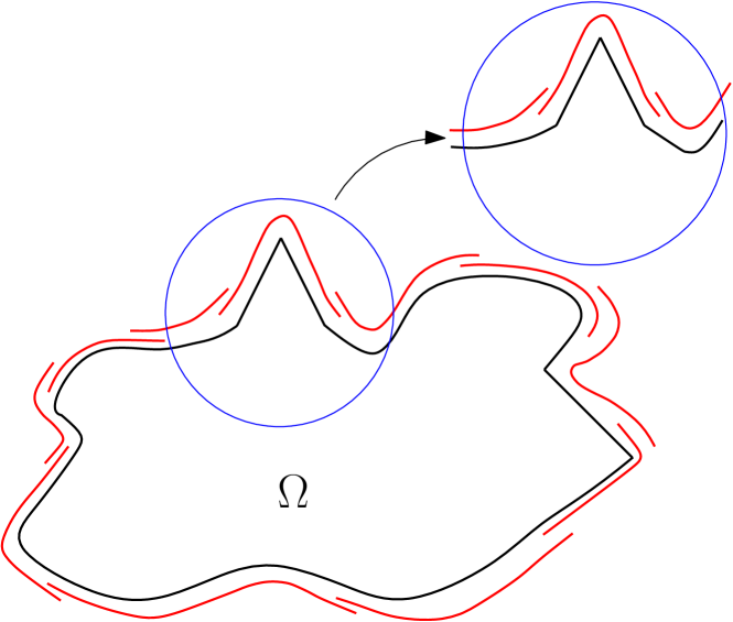
Outline of the proof. We fix a covering of , with corresponding partition of unity and local boundary charts , which are -Lipschitz continuous.
Then we regularize each function via convolution, and add (or subtract) a suitable constant, so that we obtain -smooth functions such that ( or ).
However, in the original reference system, the graphs of these smooth functions are not “glued” together, and thus their union is not the boundary of a domain, unlike the graphs whose union describes – see Figure 1 below.
To overcome this problem, we define a suitable -smooth function , built upon and – see equation (6.14) below– and define the regularized set as the sublevel set , so that
and by construction we will have .
The function is called boundary defining functions of – see [10, Section 5.4].
In order to show that is a smooth manifold, we prove that the gradient of along the directions of graphicality of is greater than a positive constant depending on – see estimate (6.20). This property of will be proven by exploiting the so-called transversality condition of , which is inherited via convolution by as well. Therefore, is strictly monotone along these directions, which entails that its zero-level set is a smooth manifold with local boundary charts defined on the same reference system as .
Thanks to the properties of convolution, we show that converge to the boundary defining function of built upon and – see equations (6.9) and (6.10)– and thus converge uniformly to .
Then, as in the proof of the implicit function theorem, we differentiate the identity , so that we may express the gradient (and its Hessian ) in terms of (and ), and then (3.4), (3.5) (and (3.6)) will be obtained by exploiting the convergence properties of convolution.
Finally, in order to get the isocapacitary estimate (3.7), we make use of the estimates on obtained in the previous steps, as to evaluate weighted Poincaré type quotients of the kind
in terms of the corresponding quotient with weight , and then (3.7) will follow from the celebrated isocapacitary equivalency Theorem of Maz’ya [15], [18, Theorem 2.4.1].
Our next and final result shows the flexibility of our approximation method, which takes into account even higher regularity of the domain .
Theorem 3.2.
Under the same notations as Theorem 3.1, we have that
-
(1)
if for some , then
-
(2)
if for some and , then
for all ;
-
(3)
if for some and , then
-
(4)
if for some , then
4. Auxiliary results
In this section, we state and prove a useful convergence property regarding the convolution of functions composed with a suitable family of bi-Lipschitz maps.
Proposition 4.1.
Let be a bounded domain, be a constant, and be a family of bi-Lipschitz maps on such that
| (4.1) |
and there exists a bi-Lipschitz map such that
| (4.2) |
Let open be such that , and for some . Then
| (4.3) |
Proof.
Set
By Lebesgue differentiation theorem and since is a bi-Lipschitz map, we have that is a subset of with full measure. Also, thanks to (4.2) and the fact that , we have that and are well defined on a neighbourhood of for large enough. Then, for all we have
Above we used the fact that is a Lebesgue point of , and as a consequence of (4.2).
Now fix , and take a function satisfying
| (4.4) |
Standard properties of convolutions ensure that
| (4.5) |
Then we have
| (4.6) |
By applying Jensen inequality, the change of variables and Fubini-Tonelli’s Theorem we obtain
We close this section recalling a variant of Lebesgue dominated convergence Theorem which will be useful later on.
Theorem 4.2 (Dominated convergence Theorem).
Let be a sequence of measurable functions on such that
-
(i)
almost everywhere on ;
-
(ii)
almost everywhere on , with for some ;
-
(iii)
there exists such that a.e. on , and .
Then , and
5. Transversality and graphicality
Throughout this section, we shall consider an isometry of , such that
| (5.1) |
where is an orthogonal matrix of , and . Let
where denotes the -th canonical vector of , i.e. , is the transpose matrix of , and is the unit sphere on .
Here we introduce the geometric notion of transversality, which was already used in [9] in a wider sense. The definition given here suffices to our purposes.
Definition 5.1 (Transversality).
Let be a Lipschitz continuous function on open. We say that a unit vector is transversal to if there exists such that
where denotes the outward normal to with respect to the subgraph .
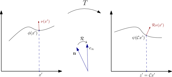
The next proposition shows a very interesting feature: the transversality of to a Lipschitz function is equivalent to the graphicality (and subgraphicality) of with respect to any reference system having , that is after performing a rotation of the axes through , the graph and subgraph of are mapped onto the graph and subgraph of another function – see identities (5.2) below.
Proposition 5.2.
Let be open, be a Lipschitz function, let be an isometry of the form (5.1), and let .
(i) If there exists an -Lipschitz function such that
| (5.2) |
then we have the transversality condition
| (5.3) |
(ii) Viceversa, if for some and (5.3) holds, then there exist open, and a function such that and (5.2) holds true.
Let us comment on this result. Part (i) states that if and are, respectively, the graph and subgraph of an -Lipschitz function with respect to the reference system having , then the quantitative transversality estimate (5.3) holds true.
Part (ii) states the opposite in the case: the transversality condition (5.3) implies the graphicality and subgraphicality of with respect to the coordinate system , and it also provides a Lipschitz estimate to .
Before starting the proof, we need to introduce the so-called transition map from to . Under the same notation as Proposition 5.2, the transition map is defined as
Here is the projection map . Observe that, when identities (5.2) hold true, by the very definition of we have the equation
In particular, this implies that is a bijection, with inverse function given by
Also, since are Lipschitz continuous, then is a bi-Lipschitz tranformation from to .
Proof of Proposition 5.2.
(i) By Rademacher’s theorem, the normal vector to outward with respect to is well defined -almost everywhere, and thanks to (5.2) and the definition of , we may write
| (5.4) |
Therefore, since and , from (5.4) we infer
| (5.5) |
(ii) Assume and that (5.3) is in force.
Consider the -function , defined as , so that
| (5.6) |
Now let be the function defined as for . Recalling , via the chain rule we compute
| (5.7) |
Thus, from expression (5.4) of and estimate (5.3), we obtain
| (5.8) |
Therefore, owing to (5.8) and the implicit function theorem, we immediately infer the existence of a function , with open, such that
Thereby, (5.2) follows from the very definition of and (5.6).
Finally, by using (5.5) we infer that for all , whence since the transition map is a bijection.
∎
Remark 5.3.
By making use of this information, we now show that the transversality condition (5.3) is inherited by the regularized function . This is the content of the following proposition
Proposition 5.4.
Let be open bounded , let be an isometry of the form (5.1), and . Let and be -Lipschitz functions satisfying (5.2). If we set
and for some sequence we define
then is -Lipschitz continuous on and
| (5.10) |
In addition, we have the transversality condition
| (5.11) |
and
| (5.12) |
where is the outward unit normal to with respect to the subgraph .
Proof.
Since we have proven that the regularized function satisfies the transversality condition, Part (ii) of Proposition 5.2 entails its “graphicality” with respect to the coordinate system having .
Proposition 5.5.
Under the same assumptions of Proposition 5.4, there exist open bounded such that
| (5.13) |
and a function satisfying
| (5.14) |
| (5.15) |
If in addition , then
| (5.16) |
and if is the transition map of , we have that
| (5.17) |
Proof.
From the results of Part (ii) of Proposition 5.2 and (5.12), there exist open bounded, and a function such that (5.15) holds. Also, owing to (5.3), we immediately obtain (5.14).
Now we recall that the transition map of is the function defined as , and for all we have
so that from (5.10) we infer
for all . In particular
| (5.18) |
The first inequality in (5.18) entails .
On the other hand, by definition of , for any we may find such that . Since and are -Lipschitz continuous, and is -Lipschitz continuous, it follows that
which implies since . Hence, by using the triangle inequality we get
that is (5.13).
Next, on assuming that , and being a bijection between and , we may take a point such that for some From (5.18) we find
and
By using these two estimates and the -Lipschitz continuity of , we obtain
that is (5.16). Finally, by making use of (5.16) and a similar argument as in the proof of (5.18), we obtain (5.17). ∎
The next proposition shows that if , then as well. Namely, graphicality preserves Sobolev second-order regularity for Lipschitz functions.
Proposition 5.6.
Proof.
Fix open, and set . Since due to (5.13), from [8, Proposition 2.2.17] we may find large enough such that
Now let
and set for . Then owing to (5.15), we have that for all . By differentiating this expression, we obtain
| (5.19) |
and from the chain rule, equation , the definition of and (5.11), we have
| (5.20) |
Moreover, thanks to (5.14) and the -Lipschitz continuity of , the maps are uniformly bi-Lipschitz, i.e.
Thanks to this piece of information and (5.17), we may apply Proposition 4.1 and get
| (5.21) |
By combining (5.19)-(5.21), and by using dominated convergence theorem, we find that converges in to some vector-valued function for all . It then follows from (5.16) and the uniqueness of the distributional limit that , hence
| (5.22) |
Next, we differentiate twice identity , and for we obtain
| (5.23) |
while from the chain rule and the properties of , we obtain
| (5.24) |
Then, another application of Proposition 4.1 entails that
in the Case . From this, (5.20), (5.22)-(5.24) and by using dominated convegence Theorem 4.2, we find that converges in to some matrix valued function . Whence due to the uniqueness of the distributional limit, and the proof in the Case is complete due to the arbitrariness of .
At last, we close this section with the following intrinsic property of domains.
Corollary 5.7.
Let be a bounded Lipschitz domains such that for some . Then any Lipschitz local chart of is of class .
Proof.
6. Proof of Theorem 3.1
This section is devoted to the proof of Theorem 3.1, which is divided into a few steps.
From here onward, and will denote positive integers, possibly changing from line to line.
6.1. Covering of
By Definition 2.1, for any , we may find an -Lipschitz function , and an isometry of such that , and
where . Let us consider the open covering of 111Any other open covering is allowed, as long as its sets are strictly contained in the coordinate cylinders . The open covering here chosen helps simplifying a few computations, especially in the isocapacitary estimate (3.7). . By compactness, we may find a finite sequence of points such that
| (6.1) |
as well as -Lipschitz functions and isometries satisfying
| (6.2) |
We denote by the orthogonal matrix of , i.e. can be written as
Notice also that the cardinality of this covering of may be chosen satisfying
| (6.3) |
We then set
so that by (6.1) we have
| (6.4) |
Starting from this point, we construct a suitable partition of unity: let
where is the standard, radially symmetric convolution kernel on , and denotes the indicator function of a set .
Standard properties of convolution ensure that , , ,
and
Therefore, by defining as
then we have that for , ,
| (6.5) |
and
| (6.6) |
6.2. Boundary defining function
Starting from the partition of unity , and the local charts , we can construct the boundary defining function of as in [10, Proposition 5.43].
For any and , we define the rotated cylinders
| (6.7) |
where . Let be the functions defined as
and observe that from (6.2) we have
| (6.8) |
A boundary defining function of is the function defined as
| (6.9) |
where the product is set equal to zero if . Since each is Lipschitz continuous, so is the function .
6.3. Regularization and definition of the smooth approximating sets
For , we can define the smooth functions as
| (6.11) | and | ||
From the results of Proposition 5.4, we deduce that are -Lipschitz functions, and
| (6.12) |
for all and . Taking inspiration from (6.8) and (6.10), we are led to define the functions
| (6.13) |
and functions defined as
| (6.14) |
where the products and have to be interpreted equal to zero when .
Clearly, and are -smooth functions on , and since
| (6.15) |
for all thanks to (6.12), we then have
| (6.16) |
The approximating open sets are thus defined as follows
| (6.17) |
with boundaries
| (6.18) |
In particular, since for all , owing to (6.10) we have
We now proceed to prove the remaining properties of Theorem 3.1 for the outer sets . The proofs for the inner sets are analogous.
6.4. are smooth manifolds .
Let us show that is a smooth manifold, with local charts defined on the same coordinate systems as .
We fix a constant , and for all we set
This piece of information will allow us to use the transversality property. Specifically, thanks to (6.19) we may apply Propositions 5.2-5.4 with functions , , isometry , and defining set
Claim 1. There exists such that, for all , for all and all , we have
| (6.20) |
Suppose by contradiction this is false; then for every , we may find and a sequence such that and
| (6.21) |
By compactness, we may extract a subsequence, still labeled as , such that , and in particular and , hence due to (6.10).
Then, by the chain rule we have
| (6.22) |
if , where .
We now distinguish two cases:
(i) is such that . Then , hence for all large enough.
(ii) is such that . In this case, it follows that , so that from (6.19) we have . By setting , we thus have
for all large enough. Recalling the remarks after (6.19), by applying Proposition 5.4, and in particular the transversality property (5.11) in (6.22), we infer
provided is large enough.
In both cases, we have found that
| (6.23) |
Also, owing to (6.15) and (6.8) we have
and since . By coupling this piece of information with (6.5), (6.21) and (6.23), we finally obtain
which is a contradiction, and thus (6.20) holds true.
Claim 2. There exists such that , , with satisfying .
Again, assume by contradiction this is false. Then for all , we may find sequences and such that
| (6.24) |
By compactness, we may find a subsequence, still labeled as , satisfying . Fix such that , and let be a sequence satisfying . Then , so that for large enough being open, and from (6.24) we have . By using (6.16) and the Lipschitz continuity of , it is readily shown that
whence for all as above, but this contradicts the fact that whenever due to (6.10), hence Claim 2 is proven.
Now let ; by (6.16) and since , we have . Thus, owing to Claim 2 we may find such that .
The monotonicity property (6.20) of Claim 1, and the fact that due to (6.16) ensure that such point is unique for all . This entails the existence of a function such that for all . Furthemore, owing to (6.10) and (6.16), we have that for all , and from the implicit function theorem we also infer that . Moreover, via a compactness argument as in Claim 1-2 and (6.1), one can prove that
| (6.25) |
so that, in particular, the cylinders are an open cover of , and provided is large enough.
We have thus proven that is a -smooth manifold for , with local boundary charts defined on the same coordinate cylinders as , that is
| (6.26) |
6.5. Approximation properties.
First, we show that there exists such that
| (6.27) |
Assume by contradiction this is false; then we may find sequences and such that
| (6.28) |
Up to a subsequence, we have , and . Furthermore, since , we readily infer that , whence due to (6.10) and (6.2). By continuity we also have , which implies that
Then, for all , we have
where denotes the Lipschitz constant of . This implies that for all large enough, the line segment
Therefore, by using (6.2), (6.10) (6.16), (6.20) and (6.28), we obtain
which is a contradiction, hence (6.27) holds true.
Now, recalling that is an open cover of and , from (6.2), (6.26) and (6.27), one can easily obtain that
This convergence property in the sense of Hausdorff immediately implies that , and –see for instance [8, Proposition 2.2.23]– and thus (3.1), (3.2) and (3.3) are proven.
Let us now introduce the transition maps related to the local charts of and .
For all , we define the set of indexes
If , then owing to (6.2) there exists such that . Since is -Lipschitz continuous and , we have , so it follows from (6.19), (6.26) and (6.27) that for all large enough.
Henceforth, for all , (6.19) and (6.29) allow us to define the transition maps from to and from to respectively, i.e.
| (6.30) |
which are defined on the open sets
In particular, by their definitions and the arguments of Section 5, we may write
| (6.31) |
and their inverse functions are and . Observe also that .
We now claim that for all , there exists an open set for which we have
| (6.33) |
and such that for all . This in particular implies that both and are defined on .
To this end, let
Then, owing to (6.27) it is immediate to verify that
| (6.34) |
whenever is large enough, and thus (6.33) is satisfied by our choice of set .
Clearly , so we are left to verify that . To this end, let ; then by (6.29) and (6.31) we may write
where in the latter inclusion we made use of the inequality . Therefore, thanks to (6.27), for we have , hence by (6.29) and the definition of , so the claim is proven.
We also remark that
| (6.35) |
since is an open cover of , and the projection map is a homeomorphism from (with the induced topology) to .
Our next goal is to obtain estimates on . To this end, we differentiate equation with respect to , for , and recalling (6.32) we find
| (6.37) |
where , .
For all , by using the chain rule and recalling the definition of , we find
| (6.38) |
for all such that . Since are -Lipschitz continuous, from (6.38) it follows that
| (6.39) |
Moreover, from (6.15), (6.27) and (6.8), we find that , where .
By making use of this piece of information, (6.39) and (6.20), from (6.37) we finally obtain the gradient estimate
| (6.40) |
for all and large enough. In particular, owing to (6.27), (6.26) and (6.40), it is readily seen that are -Lipschitz domains, with
and (3.4) is proven.
Next, the definition of and , (6.40) and the -Lipschitz continuity of imply
| (6.41) |
and in particular and are uniformly bi-Lipschitz transformations.
Hence, thanks to (6.36) and (6.41), we are in the position to apply Proposition 4.1 and get
| (6.42) |
From this, (6.20), (6.33), (6.35), (6.38) and identity (6.37) we find
where is a bounded vector valued function which can be explictly written. From (6.40) and on applying dominated convergence theorem, we get that in for all . On the other hand, (6.27) and the uniqueness of the distributional limit imply that , hence (3.5) is proven.
6.6. Curvature convergence
Assume now that for some . Then the local charts .
We differentiate twice the identity with respect to for , and find
| (6.43) |
Elementary computations and (6.32) show that, for , we have
| (6.44) |
where . We also have
| (6.45) |
for all such that .
Thanks to (6.15), (6.27) and (6.8), we readily find that and . From this, and by using (6.6), (6.20), (6.39), (6.40) and (6.43)-(6.45), we obtain
| (6.46) |
for all , provided is large enough.
Finally, recalling (6.33) and (6.35), the properties (6.20), (6.27), (6.38), (6.42), (6.43)-(6.47) and dominated convergence Theorem 4.2 entail
for some matrix valued function , which can be explictly written in terms of and . On the other hand, (6.27) and the uniqueness of the distributional limit imply that , hence (3.6) is proven.
6.7. Proof of the isocapacitary estimate (3.7)
In the following subsection, we will denote by the convolution of a function with respect to the first -variables, i.e.
We then have the following elementary lemma, which will be useful later.
Lemma 6.1.
Let . Then, if we set
we have that is Lipschitz continuous on , and
| (6.48) |
Proof.
By Hölder’s inequality, for we have
Therefore, on setting , for all we have that
| (6.49) |
Thus, the sequence is uniformly bounded in , and since on , we deduce that by weak- compactness, and the thesis follows by letting in (6.49) and by Rademacher’s Theorem. ∎
Now let ; then owing to (6.25) and (6.16), there exists such that . Therefore, we may write for some , and we also set . Let
for some fixed constant large enough, and consider , and . Then, since , we have
Consider the new set of indices
Owing to (2.8), (6.31), (6.33), (6.40) and the Hessian estimate (6.46), we obtain
| (6.50) |
By using , (6.3), (3.4) and the results of [2, Corollary 6.6], we get
| (6.51) |
On the other hand, via the change of variables , by making use of (6.41), (6.34), and observing that for all , and , we find
| (6.52) |
for some open set , where we also set
Since and for all , by using (6.40) it is readily seen that
and from the chain rule we find
| (6.53) |
Next, by using Fubini-Tonelli’s Theorem we obtain
We have thus found that
| (6.54) |
for some open set , provided is large enough.
Thanks to Lemma 6.1 and inequality (6.36), we easily infer
and
| (6.55) |
Finally, set
so that is Lipschitz continuous on . Moreover, thanks to (6.27), for all , we have that
for all sufficiently large and all , and thus we may write due to (6.31). Recalling that is -Lipschitz continous, it follows that
and from the chain rule
| (6.56) |
Owing to (2.8) and the definition of , we have
| (6.57) |
where the supremum above is taken over all functions .
Henceforth, by coupling (6.3) and estimates (6.50)-(6.57), for all we obtain
where in the second inequality we made use of Fubini-Tonelli’s Theorem, the supremum above is taken over all , and we set
| (6.58) |
Therefore, for all , , we have found
From this, (6.58) and the isocapacitary equivalence [18, Theorem 2.4.1], we finally obtain the desired estimate
| (6.59) |
for all and , and the proof is complete.
Acknowledgments
I would like to thank professors A. Cianchi, G. Ciraolo and A. Farina for suggesting the problem, and for useful discussions and observations on the topic.
The author has been partially supported by the “Gruppo Nazionale per l’Analisi Matematica, la Probabilità e le loro Applicazioni” (GNAMPA) of the “Istituto Nazionale di Alta Matematica” (INdAM, Italy).
Data availability statement. Data sharing not applicable to this article as no datasets were generated or analysed during the current study.
References
- [1] L. Ambrosio, N. Fusco, D. Pallara, Functions of bounded variation and free discontinuity problems, Oxford Mathematical Monographs. The Clarendon Press, Oxford University Press, New York, 2000. xviii+434 pp.
- [2] C.A. Antonini, A. Cianchi, G. Ciraolo, A. Farina, V.G. Maz’ya, Global second-order estimates in anisotropic elliptic problems, arXiv preprint (2023) arXiv:2307.03052.
- [3] A. Kh. Balci, A. Cianchi, L. Diening, V. G. Maz’ya, A pointwise differential inequality and second-order regularity for nonlinear elliptic systems, Math. Ann. 383 (2022), no. 3-4, 1775-1824
- [4] J. M. Ball, A. Zarnescu, Partial regularity and smooth topology-preserving approximations of rough domains, Calc. Var. Partial Differential Equations 56 (2017), no. 1, Paper No. 13, 32 pp.
- [5] A. Cianchi, V.G. Maz’ya, Optimal second-order regularity for the -Laplace system, J. Math. Pures Appl. (9) 132 (2019), 41-78.
- [6] P. Doktor, Approximation of domains with Lipschitzian boundary, Časopis Pěst. Mat. 101 (1976), no. 3, 237-255.
- [7] C. Gui, Y. Hu, Q. Li, On smooth interior approximation of sets of finite perimeter, Proc. Amer. Math. Soc. 151 (2023), no. 5, 1949-1962.
- [8] A. Henrot, M. Pierre, Shape variation and optimization, European Mathematical Society (EMS), Zürich, 2018. xi+365 pp.
- [9] S. Hofmann, M. Mitrea, T. Michael, Geometric and transformational properties of Lipschitz domains, Semmes-Kenig-Toro domains, and other classes of finite perimeter domains, J. Geom. Anal. 17 (2007), no. 4, 593-647.
- [10] J.M. Lee, Introduction to smooth manifolds, Second edition. Graduate Texts in Mathematics, 218. Springer, New York, 2013. xvi+708 pp.
- [11] J.M. Lee, Introduction to Riemannian manifolds, Second edition, Graduate Texts in Mathematics, 176. Springer, Cham, 2018. xiii+437 pp.
- [12] G. M. Lieberman, Regularized distance and its applications, Pacific J. Math. 117 (1985), no. 2, 329-352
- [13] F. Maggi, Sets of finite perimeter and geometric variational problems, An introduction to geometric measure theory. Cambridge Studies in Advanced Mathematics, 135. Cambridge University Press, Cambridge, 2012. xx+454 pp.
- [14] U. Massari, L. Pepe, Sull’approssimazione degli aperti lipschitziani di con varietá differenziabili, Boll. Un. Mat. Ital. (4) 10 (1974), 532-544.
- [15] V.G. Maz’ya, -conductivity and theorems on imbedding certain functional spaces into a -space, Dokl. Akad. Nauk SSSR 140 (1961), 299-302.
- [16] V. G. Maz’ya, Solvability in of the Dirichlet problem in a region with a smooth irregular boundary, Vestnik Leningrad. Univ. 22 (1967), no. 7, 87-95.
- [17] V. G. Maz’ya, The coercivity of the Dirichlet problem in a domain with irregular boundary, Izv. Vyss̆. Uc̆ebn. Zaved. Matematika (1973), no. 4 (131), 64-76.
- [18] V. G. Maz’ya, Sobolev spaces with applications to elliptic partial differential equations, Grundlehren der mathematischen Wissenschaften [Fundamental Principles of Mathematical Sciences] 342, Springer, Heidelberg, 2011, xxviii+866.
- [19] J. Nečas, On domains of type , Czechoslovak Math. J. 12 (87) (1962), 274-287.
- [20] T. Schmidt, Strict interior approximation of sets of finite perimeter and functions of bounded variation, Proc. Amer. Math. Soc. 143 (2015), no. 5, 2069-2084.