Expressive Modeling Is Insufficient for
Offline RL: A Tractable Inference Perspective

Abstract

A popular paradigm for offline Reinforcement Learning (RL) tasks is to first fit the offline trajectories to a sequence model, and then prompt the model for actions that lead to high expected return. While a common consensus is that more expressive sequence models imply better performance, this paper highlights that tractability, the ability to exactly and efficiently answer various probabilistic queries, plays an equally important role. Specifically, due to the fundamental stochasticity from the offline data-collection policies and the environment dynamics, highly non-trivial conditional/constrained generation is required to elicit rewarding actions. While it is still possible to approximate such queries, we observe that such crude estimates significantly undermine the benefits brought by expressive sequence models. To overcome this problem, this paper proposes Trifle (Tractable Inference for Offline RL), which leverages modern Tractable Probabilistic Models (TPMs) to bridge the gap between good sequence models and high expected returns at evaluation time. Empirically, Trifle achieves the most state-of-the-art scores in $9$ Gym-MuJoCo benchmarks against strong baselines. Further, owing to its tractability, Trifle significantly outperforms prior approaches in stochastic environments and safe RL tasks (e.g., with action constraints) with minimum algorithmic modifications.

1 Introduction

Recent advancements in deep generative models have opened up the possibility of solving offline Reinforcement Learning (RL) (Levine et al., 2020) tasks with sequence modeling techniques (termed RvS approaches). Specifically, we first fit the trajectories provided in an offline dataset to a sequence model. During evaluation, the model is tasked to sample actions with high expected returns given the current state. Leveraging modern deep generative models such as GPTs (Brown et al., 2020) and diffusion models (Ho et al., 2020), RvS algorithms have significantly boosted the performance on various discrete/continuous control problems (Ajay et al., 2022; Chen et al., 2021).

Despite its appealing simplicity, it is still unclear whether expressive modeling alone guarantees good performance of RvS algorithms, and if so, on what types of environments. Perhaps surprisingly, this paper discovers that many common failures of RvS algorithms are not caused by modeling problems. Instead, while useful information is encoded in the model during training, the model is unable to elicit such knowledge during evaluation. Specifically, this issue is reflected in two aspects: (i) inability to accurately estimate the expected return of a state and a corresponding action sequence to be executed given near-perfect learned transition dynamics and reward functions; (ii) even when accurate return estimates exist in the offline dataset and are learned by the model, it could still fail to sample rewarding actions during evaluation. At the heart of such inferior evaluation-time performance is the fact that highly non-trivial conditional/constrained generation is required to stimulate high-return actions (Paster et al., 2022; Brandfonbrener et al., 2022). Therefore, other than expressiveness, the ability to efficiently and exactly answer various queries (e.g., computing the expected cumulative rewards), termed tractability, plays an equally important role in RvS approaches.

Having observed that the lack of tractability is an essential cause of the underperformance of RvS algorithms, this paper studies whether we can gain practical benefits from using Tractable Probabilistic Models (TPMs) (Poon & Domingos, 2011; Choi et al., 2020; Kisa et al., 2014), which by design support exact and efficient computation of certain queries? We answer the question in its affirmative by showing that we can leverage a class of TPMs that support computing arbitrary marginal probabilities to significantly mitigate the inference-time suboptimality of RvS approaches. The proposed algorithm Trifle (Tractable Inference for Offline RL) has three main contributions:

Emphasizing the important role of tractable models in offline RL. This is the first paper that demonstrates the possibility of using TPMs on complex offline RL tasks. The superior empirical performance of Trifle suggests that expressive modeling is not the only aspect that determines the performance of RvS algorithms, and motivates the development of better inference-aware RvS approaches.

Competitive empirical performance. Compared against strong offline RL baselines (including RvS, imitation learning, and offline temporal-difference algorithms), Trifle achieves the most state-of-the-art scores on $9$ Gym-MuJoCo benchmarks (Fu et al., 2020).

Generalizability to stochastic environments and safe-RL tasks. Trifle can be extended to tackle stochastic environments as well as safe RL tasks with minimum algorithmic modifications. Specifically, we evaluate Trifle in a stochastic Taxi environment and action-space-constrained MuJoCo environments, and demonstrate superior performance against all baselines.

2 Preliminaries

Offline Reinforcement Learning

In Reinforcement Learning (RL), an agent interacts with an unknown environment at discrete time steps to maximize its cumulative reward. The environment is defined by a Markov Decision Process (MDP) $\langle\mathcal{S},\mathcal{A},\mathcal{R},\mathcal{P},d_{0}\rangle$, where $\mathcal{S}$ is the state space, $\mathcal{A}$ is the action space, $\mathcal{R}:\mathcal{S}\times\mathcal{A}\rightarrow\mathbb{R}$ is the reward function, $\mathcal{P}:\mathcal{S}\times\mathcal{A}\rightarrow\mathcal{S}$ is the transition dynamics, and $d_{0}$ is the initial state distribution. Our goal is to learn a policy $\pi(a|s)$ that maximizes the expected return $\mathbb{E}[\sum_{t=0}^{T}\gamma^{t}r_{t}]$, where $\gamma\in(0,1]$ is a discount factor and $T$ is the maximum number of steps.

Offline RL (Levine et al., 2020) aims to solve RL problems where we cannot freely interact with the environment. Instead, we receive a dataset of trajectories collected using unknown policies. An effective learning paradigm for offline RL is to treat it as a sequence modeling problem (termed RL via Sequence Modeling or RvS methods) (Janner et al., 2021; Chen et al., 2021; Emmons et al., 2021). Specifically, we first learn a sequence model on the dataset, and then sample actions conditioned on past states and high future returns. Since the models typically do not encode the entire trajectory, an estimated value or return-to-go (RTG) (i.e., the Monte Carlo estimate of the sum of future rewards) is also included for every state-action pair, allowing the model to estimate the return at any time step.

Tractable Probabilistic Models

Tractable Probabilistic Models (TPMs) are generative models that are designed to efficiently and exactly answer a wide range of probabilistic queries (Poon & Domingos, 2011; Choi et al., 2020; Rahman et al., 2014). One example class of TPMs is Hidden Markov Models (HMMs) (Rabiner & Juang, 1986), which support linear time (w.r.t. model size and input size) computation of marginal probabilities and more. Recent advancements have extensively pushed forward the expressiveness of modern TPMs (Liu et al., 2022; 2023; Correia et al., 2023), leading to competitive likelihoods on natural image and text datasets compared to even strong Variational Autoencoder (Vahdat & Kautz, 2020) and Diffusion model (Kingma et al., 2021) baselines. This paper leverages such advances and explores the benefits brought by TPMs in offline RL tasks.

3 Tractability Matters in Offline RL

Practical RvS approaches operate in two main phases – training and evaluation. In the training phase, a sequence model is adopted to learn a joint distribution over trajectories of length $T$: $\{(s_{t},a_{t},r_{t},\mathrm{RTG}_{t})\}_{t=0}^{T}$. During evaluation, at every time step $t$, the model is tasked to discover an action sequence $a_{t:T}:=\{a_{\tau}\}_{\tau=t}^{T}$ (or just $a_{t}$) that has high expected return as well as high probability in the prior policy ${p}(a_{t:T}|s_{t})$, which prevents it from generating out-of-distribution actions:

$${p}(a_{t:T}|s_{t},\mathbb{E}[V_{t}]\geq v):=\frac{1}{Z}\cdot\begin{cases}{p}(a_{t:T}|s_{t})&\text{if~{}}\mathbb{E}_{V_{t}\sim{p}(\cdot|s_{t},a_{t})}[V_{t}]\geq v,\\ 0&\text{otherwise},\end{cases}$$ (1)

where $Z$ is a normalizing constant, $V_{t}$ is an estimate of the value at time step $t$, and $v$ is a pre-defined scalar whose value is chosen to encourage high-return policies. Depending on the problem, $V_{t}$ could be the labeled RTG from the dataset (e.g., $\mathrm{RTG}_{t}$) or the sum of future rewards capped with a value estimate (e.g., $\sum_{\tau=t}^{T-1}r_{\tau}+\mathrm{RTG}_{T}$) (Emmons et al., 2021; Janner et al., 2021).

The above definition naturally reveals two key challenges in RvS approaches: (i) training-time optimality: how well can we fit the offline trajectories, and (ii) inference-time optimality: whether actions can be unbiasedly and efficiently sampled from Equation 1. While extensive breakthroughs have been achieved to improve the training-time optimality (Ajay et al., 2022; Chen et al., 2021; Janner et al., 2021), it remains unclear whether the non-trivial constrained/conditional generation task of Equation 1 hinders inference-time optimality. In the following, we present two general scenarios where existing RvS approaches underperform as a result of suboptimal inference-time performance. We attribute such failures to the fact that these models are limited to answering certain query classes (e.g., autoregressive models can only compute next token probabilities), and explore the potential of tractable probabilistic models for offline RL tasks in the following sections.

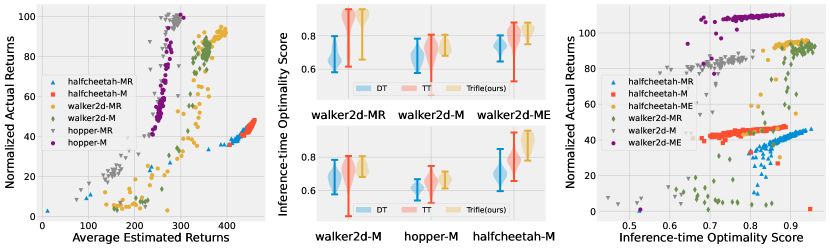
Figure 1: RvS approaches suffer from inference-time suboptimality. Left: There exists a strong positive correlation between the average estimated returns by Trajectory Transformers (TT) and the normalized actual returns in 6 Gym-MuJoCo environments (MR, M, and ME are short for medium-replay, medium, and medium-expert, respectively), which suggests that the sequence model can distinguish rewarding actions from bad ones. Middle: Despite being able to recognize high-return actions, both TT and DT (Chen et al., 2021) fail to consistently sample such action, leading to bad inference-time optimality; our method Trifle consistently improves the inference-time optimality score. Right: We substantiate the relationship between low inference-time optimality scores and unfavorable environmental outcomes by showing a strong positive correlation between them.

Scenario #1   We first consider the case where the labeled RTG belongs to a (near-)optimal policy. In this case, Equation 1 can be simplified to ${p}(a_{t}|s_{t},\mathbb{E}[V_{t}]\geq v)$ (choose $V_{t}:=\mathrm{RTG}_{t}$) since one-step optimality implies multi-step optimality. In practice, although the RTGs are suboptimal, the predicted values often match well with the actual returns achieved by the agent. Take Trajectory Transformer (TT) (Janner et al., 2021) as an example, Figure 1 (left) demonstrates a strong positive correlation between its predicted returns (x-axis) and the actual cumulative rewards (y-axis) on six MuJoCo (Todorov et al., 2012) benchmarks, suggesting that the model has learned the “goodness” of most actions. In such cases, the performance of RvS algorithms depends mainly on their inference-time optimality, i.e., whether they can efficiently sample actions with high predicted returns. Specifically, let $a_{t}$ be the action taken by a RvS algorithm at state $s_{t}$, and $R_{t}:=\mathbb{E}[\mathrm{RTG}_{t}]$ is the corresponding estimated expected value. We define a proxy of inference-time optimality as the quantile value of $R_{t}$ in the estimated state-conditioned value distribution ${p}(V_{t}|s_{t})$. The higher the quantile value, the more frequent the RvS algorithm samples actions with high estimated returns.

We evaluate the inference-time optimality of Decision Transformers (DT) (Chen et al., 2021) and Trajectory Transformers (TT) (Janner et al., 2021), two widely used RvS algorithms, on various environments and offline datasets from the Gym-MuJoCo benchmark suite (Fu et al., 2020). Perhaps surprisingly, as shown in Figure 1 (middle), the inference-time optimality is averaged (only) around $0.7$ (the maximum possible value is $1.0$) for most settings. And these runs with low inference-time optimality scores receive low environment returns (Fig. 1 (right)).

Scenario #2   Achieving inference-time optimality becomes even harder when the labeled RTGs are suboptimal (e.g., they come from a random policy). In this case, even estimating the expected future return of an action sequence becomes highly intractable, especially when the transition dynamics of the environment are stochastic. Specifically, to evaluate a state-action pair $(s_{t},a_{t})$, since $\mathrm{RTG}_{t}$ is uninformative, we need to resort to the multi-step estimate $V_{t}^{\mathrm{m}}:=\sum_{\tau=t}^{t^{\prime}-1}r_{\tau}+\mathrm{RTG}_{t^{\prime}}$ ($t^{\prime}>t$), where the actions $a_{t:t^{\prime}}$ are jointly chosen to maximize the expected return. Take autoregressive models as an example. Since the variables are arranged following the sequential order $\dots,s_{t},a_{t},r_{t},\mathrm{RTG}_{t},s_{t+1},\dots$, we need to explicitly sample $s_{t+1:t^{\prime}}$ before proceed to compute the rewards and the RTG in $V_{t}^{\mathrm{m}}$. When the transition dynamics are stochastic, estimating $\mathbb{E}[V_{t}^{\mathrm{m}}]$ could suffer from high variance as the stochasticity from the intermediate states accumulates over time.

As we shall illustrate in Section 6.2, compared to environments with near-deterministic transition dynamics (e.g., Fig. 1 (left)), estimating the expected returns in stochastic environments using intractable sequence models is hard, and Trifle can significantly mitigate this problem with its ability to marginalize out intermediate states and compute $\mathbb{E}[V_{t}^{\mathrm{m}}]$ in closed-form.

4 Exploiting Tractable Models

The previous section demonstrates that apart from modeling, inference-time suboptimality is another key factor that causes the underperformance of RvS approaches. Given such observations, a natural follow-up question is whether/how more tractable models can improve the evaluation-time performance in offline RL tasks? While there are different types of tractabilities (i.e., the ability to compute different types of queries), this paper focuses on studying the additional benefit of exactly computing arbitrary marginal/condition probabilities. This strikes a proper balance between learning and inference as we can train such a tractable yet expressive model thanks to recent developments in the TPM community (Liu et al., 2022; Correia et al., 2023). Note that in addition to proposing a competitive RvS algorithm, we aim to highlight the necessity and benefit of using more tractable models for offline RL tasks, and encourage future developments on both inference-aware RvS methods and better TPMs. As a direct response to the two failing scenarios identified in Section 3, in the following, we first demonstrate how tractability could help even when the labeled RTGs are (near-)optimal (Sec. 4.1). We then move on to the more general case where we need to use multi-step return estimates to account for biases in the labeled RTGs (Sec. 4.2).

4.1 From the Single-Step Case…

Consider the case where the RTGs are optimal. Recall from Section 3 that our goal is to sample actions from ${p}(a_{t}|s_{t},\mathbb{E}[V_{t}]\geq v)$ ($V_{t}:=\mathrm{RTG}_{t}$). Prior works use two typical ways to approximately sample from this distribution. The first approach directly trains a model to generate return-conditioned actions: ${p}(a_{t}|s_{t},\mathrm{RTG}_{t})$ (Chen et al., 2021). However, since the RTG given a state-action pair is stochastic, sampling from this RTG-conditioned policy could result in actions with a small probability of getting a high return, but with a low expected return (Paster et al., 2022; Brandfonbrener et al., 2022).

An alternative approach leverages the ability of sequence models to accurately estimate the expected return (i.e., $\mathbb{E}[\mathrm{RTG}_{t}]$) of state-action pairs (Janner et al., 2021). Specifically, we first sample from a prior distribution ${p}(a_{t}|s_{t})$, and then reject actions with low expected returns. Such rejection sampling-based methods typically work well when the action space is small (in which we can enumerate all actions) or the dataset contains many high-rewarding trajectories (in which the rejection rate is low). However, the action could be multi-dimensional and the dataset typically contains many more low-return trajectories in practice, rendering the inference-time optimality score low (cf. Fig. 1).

Having examined the pros and cons of existing approaches, we are left with the question of whether a tractable model can improve sampled actions (in this single-step case). We answer it with a mixture of positive and negative results: while computing ${p}(a_{t}|s_{t},\mathbb{E}[V_{t}]\geq v)$ is NP-hard even when ${p}(a_{t},V_{t}|s_{t})$ follows a simple Naive Bayes distribution, we can design an approximation algorithm that samples high-return actions with high probability in practice. We start with the negative result.

Theorem 1.

Let $a_{t}:=\{a_{t}^{i}\}_{i=1}^{k}$ be a set of $k$ boolean variables and $V_{t}$ be a categorical variables with two categories $0$ and $1$. For some $s_{t}$, assume the joint distribution over $a_{t}$ and $V_{t}$ conditioned on $s_{t}$ follows a Naive Bayes distribution: ${p}(a_{t},V_{t}|s_{t}):={p}(V_{t}|s_{t})\cdot\prod_{i=1}^{k}{p}(a_{t}^{i}|V_{t},s_{t})$, where $a_{t}^{i}$ denotes the $i$th variable of $a_{t}$. Computing ${p}(a_{t}|s_{t},\mathbb{E}[V_{t}]\geq v)$ is NP-hard.

The proof is given in Appx. A. While it seems hard to directly draw samples from ${p}(a_{t}|s_{t},\mathbb{E}[V_{t}]\geq v)$, we propose to improve the aforementioned rejection sampling-based method by adding a correction term to the original proposal distribution ${p}(a_{t}|s_{t})$ to reduce the rejection rate. Specifically, the prior is often represented by an autoregressive model such as GPT: ${p}_{\mathrm{GPT}}(a_{t}|s_{t}):=\prod_{i=1}^{k}{p}_{\mathrm{GPT}}(a_{t}^{i}|s_{t},a_{t}^{<i})$, where $k$ is the number of action variables and $a_{t}^{i}$ is the $i$th variable of $a_{t}$. We sample every dimension of $a_{t}$ autoregressively following:

$$\forall i\in\{1,\dots,k\}\quad\tilde{{p}}(a_{t}^{i}|s_{t},a_{t}^{<i};v):=\frac{1}{Z}\cdot{p}_{\mathrm{GPT}}(a_{t}^{i}|s_{t},a_{t}^{<i})\cdot{p}_{\mathrm{TPM}}(V_{t}\geq v|s_{t},a_{t}^{\leq i}),$$ (2)

where $Z$ is a normalizing constant and ${p}_{\mathrm{TPM}}(V_{t}\geq v|s_{t},a_{t}^{\leq i})$ is a correction term that leverages the ability of the TPM to compute the distribution of $V_{t}$ given incomplete actions. Note that while Equation 2 is mathematically identical to ${p}(a_{t}|s_{t},V_{t}\geq v)$, this formulation gives us the flexibility to use the prior policy (i.e., ${p}_{\mathrm{GPT}}(a_{t}^{i}|s_{t},a_{t}^{<i})$) represented by more expressive autoregressive generative models. Further, as shown in Figure 1 (middle), compared to using ${p}(a_{t}|s_{t})$ (as done by TT), the inference-time optimality scores increase significantly when using the distribution specified by Equation 2 (as done by Trifle) across various Gym-MuJoCo benchmarks.

4.2 …To the Multi-Step Case

Recall that when the labeled RTGs are suboptimal, our goal is to sample from ${p}(a_{t:t^{\prime}}|s_{t},\mathbb{E}[V_{t}^{\mathrm{m}}]\!\geq\!v)$ ($t^{\prime}>t$), where $V_{t}^{\mathrm{m}}:=\sum_{\tau=t}^{t^{\prime}-1}r_{\tau}+\mathrm{RTG}_{t^{\prime}}$ is the multi-step value estimate. However, as elaborated in the second scenario in Section 3, it is hard even to evaluate the expected return of an action sequence due to the inability to marginalize out intermediate states $s_{t+1:t^{\prime}}$. Empowered by TPMs, we can readily solve this problem thanks to the linearity of the expectation operator:

$$\mathbb{E}\big{[}V_{t}^{\mathrm{m}}\big{]}=\sum_{\tau=t}^{t^{\prime}-1}\mathbb{E}_{r_{\tau}\sim{p}(\cdot|s_{t},a_{t:t^{\prime}})}\big{[}r_{\tau}\big{]}+\mathbb{E}_{\mathrm{RTG}_{t^{\prime}}\sim{p}(\cdot|s_{t},a_{t:t^{\prime}})}\big{[}\mathrm{RTG}_{t^{\prime}}\big{]}.$$

We are now left with the same problem discussed in the single-step case — how to sample actions with high expected returns (i.e., $\mathbb{E}[V_{t}^{\mathrm{m}}]$). Following Equation 2, we sample potentially rewarding actions by conditioning the action sequence on $V_{t}^{\mathrm{m}}\geq v$:

$$\tilde{{p}}(a_{t:t^{\prime}}|s_{t};v)\!:=\!\prod_{\tau=t}^{t^{\prime}}\tilde{{p}}(a_{\tau}|s_{t},a_{<\tau};v),\text{~{}where~{}}\,\tilde{{p}}(a_{\tau}|s_{t},a_{<\tau};v)\propto{p}(a_{\tau}|s_{t},a_{<\tau}\!)\cdot{p}(V_{t}^{\mathrm{m}}\!\geq\!v|s_{t},a_{\leq\tau}\!),$$

$a_{<\tau}$ and $a_{\leq\tau}$ represent $a_{t:\tau-1}$ and $a_{t:\tau}$, respectively. In practice, while we compute ${p}(V_{t}\geq v|s_{t},a_{\leq\tau})$ using the TPM, ${p}(a_{\tau}|s_{t},a_{<\tau})=\mathbb{E}_{s_{t+1:\tau}}[{p}(a_{\tau}|s_{\leq\tau},a_{<\tau})]$ can either be computed exactly with the TPM or approximated (via Monte Carlo estimation over $s_{t+1:\tau}$) using an autoregressive neural network. In summary, we approximate samples from ${p}(a_{t:t^{\prime}}|s_{t},\mathbb{E}[V_{t}]\geq v)$ by first sampling from $\tilde{{p}}(a_{t:t^{\prime}}|s_{t};v)$, and then rejecting samples whose (predicted) expected return is smaller than $v$.

5 Practical Implementation with TPMs

The previous section has demonstrated how to efficiently sample from the expected-value-conditioned policy (Eq. 1). Based on this sampling algorithm, this section further introduces the proposed algorithm Trifle (Tractable Inference for Offline RL). The high-level idea of Trifle is to obtain good action (sequence) candidates from ${p}(a_{t}|s_{t},\mathbb{E}[V]\geq v)$, and then use beam search to further single out the most rewarding action. Intuitively, by the definition in Equation 1, the candidates are both rewarding and have relatively high likelihoods in the offline dataset, which ensures the actions are within the offline data distribution and prevents overconfident estimates during beam search.

Beam search maintains a set of $N$ (incomplete) sequences each starting as an empty sequence. For ease of presentation, we assume the current time step is $0$. At every time step $t$, beam search replicates each of the $N$ actions sequences into $\lambda\in\mathbb{Z}^{+}$ copies and appends an action $a_{t}$ to every sequence. Specifically, for every partial action sequence $a_{<t}$, we sample an action following ${p}(a_{t}|s_{0},a_{<t},\mathbb{E}[V_{t}]\geq v)$, where $V_{t}$ can be either the single-step or the multi-step estimate depending on the task. Now that we have $\lambda\cdot N$ trajectories in total, the next step is to evaluate their expected return, which can be computed exactly using the TPM (see Sec. 4.2). The $N$-best action sequences are kept and proceed to the next time step. After repeating this procedure for $H$ time steps, we return the best action sequence. The first action in the sequence is used to interact with the environment.

Another design choice is the threshold value $v$. While it is common to use a fixed high return throughout the episode, we follow Ding et al. (2023) and use an adaptive threshold. Specifically, at state $s_{t}$, we choose $v$ to be the $\epsilon$-quantile value of ${p}(V_{t}|s_{t})$, which is computed using the TPM.

Details of the adopted TPM   This paper uses Probabilistic Circuits (PCs) (Choi et al., 2020) as an example TPM to demonstrate the effectiveness of Trifle. PCs can compute any marginal or conditional probability in time linear with respect to its size. We use a state-of-the-art PC structure called HCLT (Liu & Van den Broeck, 2021) and optimize its parameters using the latent variable distillation technique (Liu et al., 2022). Additional training/inference details are provided in Appx. B.

6 Experiments

This section takes gradual steps to study whether Trifle can mitigate the inference-time suboptimality problem in different settings. First, in the case where the labeled RTGs are good performance indicators (i.e., the single-step case), we examine whether Trifle can consistently sample more rewarding actions (Sec. 6.1). Next, we further challenge Trifle in highly stochastic environments, where existing RvS algorithms fail catastrophically due to the failure to account for the environmental randomness (Sec. 6.2). Finally, we demonstrate that Trifle can be directly applied to safe RL tasks (with action constraints) by effectively conditioning on the constraints being satisfied (Sec. 6.3). Collectively, this section highlights the potential of TPMs on offline RL tasks.

6.1 Comparison with the State of the Art

Table 1: Normalized Scores on the standard Gym-MuJoCo benchmarks. The results of Trifle are averaged over 12 random seeds, and mean as well as standard deviations are reported. Results of the baselines are acquired from their respective papers. “$\#$ Wins of Trifle” denotes the number of environments out of 9 where Trifle outperforms each baseline. Bold indicates the best result.

Dataset	Environment	RvS					IL			Offline-TD
		Trifle	BR-RCRL	DD	TT	DT	BC	10%BC	TD3+BC	IQL	CQL	BEAR
Med-Expert	HalfCheetah	95.1$\pm$0.3	95.2	90.6	95.0	86.8	55.2	92.9	90.7	86.7	91.6	53.4
Med-Expert	Hopper	113.0$\pm$0.4	112.9	111.8	110.0	107.6	52.5	110.9	98.0	91.5	105.4	96.3
Med-Expert	Walker2d	109.3$\pm$0.1	111.0	108.8	101.9	108.1	107.5	109.0	110.1	109.6	108.8	40.1
Medium	HalfCheetah	49.5$\pm$0.2	48.6	49.1	46.9	42.6	42.6	42.5	48.3	47.4	44.0	41.7
Medium	Hopper	67.1$\pm$4.3	78.0	79.3	61.1	67.6	52.9	56.9	59.3	66.3	58.5	52.1
Medium	Walker2d	83.1$\pm$0.8	82.3	82.5	79.0	74.0	75.3	75.0	83.7	78.3	72.5	59.1
Med-Replay	HalfCheetah	45.0$\pm$0.3	42.3	39.3	41.9	36.6	36.6	40.6	44.6	44.2	45.5	38.6
Med-Replay	Hopper	97.8$\pm$0.3	98.3	100.0	91.5	82.7	18.1	75.9	60.9	94.7	95.0	33.7
Med-Replay	Walker2d	88.3$\pm$3.8	80.6	75.0	82.6	66.6	26.0	62.5	81.8	73.9	77.2	19.2
# Wins of Trifle		Reference	5	7	9	8	9	9	8	8	8	9

As demonstrated in Section 3 and Figure 1, although the labeled RTGs in the Gym-MuJoCo (Fu et al., 2020) benchmarks are accurate enough to reflect the actual environmental return, existing RvS algorithms fail to effectively sample such actions due to their large and multi-dimensional action space. Figure 1 (middle) has demonstrated that Trifle achieves better inference-time optimality. This section further examines whether higher inference-time optimality scores lead to better performance.

Environment setup   The Gym-MuJoCo benchmark suite collects trajectories in $3$ locomotion environments (HalfCheetah, Hopper, Walker2D) and constructs $3$ datasets (Medium-Expert, Medium, Medium-Replay) for every environment, which results in $3\times 3=9$ tasks. For every environment, the main difference between the datasets is the quality of its trajectories. Specifically, the dataset “Medium” records 1 million steps collected from a Soft Actor-Critic (SAC) (Haarnoja et al., 2018) agent. The “Medium-Replay” dataset contains all samples in the replay buffer recorded during the training process of the SAC agent. The “Medium-Expert” dataset mixes 1 million steps of expert demonstrations and 1 million suboptimal steps generated by a partially trained SAC policy or a random policy. The results are normalized to ensure that the well-trained SAC model has a 100 score and the random policy has a 0 score.

Baselines   We compare Trifle against three main classes of offline RL methods: (i) RvS approaches including Trajectory Transformer (TT) (Janner et al., 2021), Decision Transformer (DT) (Chen et al., 2021), Decision Diffuser (DD) (Ajay et al., 2022), and Bayesian Reprameterized RCRL (BR-RCRL) (Ding et al., 2023); (ii) Offline TD learning methods (Offline-TD) including IQL (Kostrikov et al., 2021), CQL (Kumar et al., 2020), and BEAR (Kumar et al., 2019a); (iii) Imitation learning methods (IL) that do not explicitly encode reward or value information. Specifically, we consider Behavior Cloning (BC) (Pomerleau, 1988), its variant 10% BC which only uses 10% of trajectories with the highest return, and TD3+BC (Fujimoto et al., 2019) for comparison.

Since the labeled RTGs are informative enough about the “goodness” of actions, we implement Trifle by adopting the single-step value estimate (i.e., $V_{t}=\mathrm{RTG}_{t}$), for both the action evaluation step and the action sampling step as described in Section 5. See Section C.1 for more algorithmic details.

Empirical Insights   Results are shown in Table 1. First, Trifle achieves the most state-of-the-art scores and especially performs well in Med-Replay datasets which consist of much more suboptimal trajectories compared to the two other types of datasets. Next, compared to every individual baseline, Trifle achieves better results in $5$ to $9$ out of $9$ benchmarks. To further examine the benefit brought by TPMs, we compare Trifle with TT since in this setup, their main algorithmic difference is the use of the improved proposal distribution (Eq. 2) for sampling actions. We can see that Trifle outperforms TT by a large margin in all environments, indicating that Trifle can robustly sample better actions from the high-dimensional action space.

6.2 A Stochastic Environment: The Modified Gym-Taxi Environment

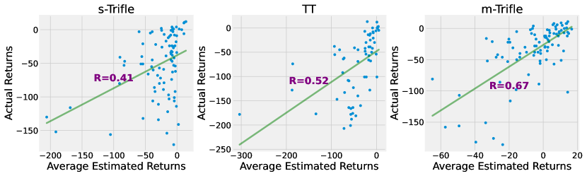
Figure 2: Correlation between average estimated returns and true environmental returns for s-Trifle (w/ single-step value estimates), TT, and m-Trifle (w/ multi-step value estimates) in the stochastic Taxi domain. $R$ denotes the correlation coefficient. The results demonstrate that (i) multi-step value estimates (TT and m-Trifle) are better than single-step estimates (s-Trifle), and (ii) exactly computed multi-step estimates (m-Trifle) are better than approximated ones (TT) in stochastic environments.

This section further challenges Trifle on stochastic environments with highly suboptimal trajectories as well as labeled RTGs in the offline dataset. As demonstrated in Section 3, in this case, it is even hard to obtain accurate value estimates due to the stochasticity of transition dynamics. Section 4.2 demonstrates the potential of Trifle to more reliably estimate and sample action sequences under suboptimal labeled RTGs and stochastic environments. This section examines this claim by comparing the four following algorithms: (i) Trifle that adopts $V_{t}=\mathrm{RTG}_{t}$ (termed single-step Trifle or s-Trifle); (ii) Trifle equipped with $V_{t}=\sum_{\tau=t}^{t^{\prime}}r_{\tau}+\mathrm{RTG}_{t^{\prime}}$ (termed multi-step Trifle or m-Trifle); (iii) Trajectory Transformers (TT) (Janner et al., 2021); (iv) Decision Transformers (DT) (Chen et al., 2021). Among the four algorithms, s-Trifle and DT do not compute the “more accurate” multi-step value, and TT approximates the value by Monte Carlo samples. Therefore, we expect their relative performance to be $\text{DT}\approx\text{s-Trifle}<\text{TT}<\text{m-Trifle}$.

Environment setup   We create a stochastic variant of the Gym-Taxi Environment (Dietterich, 2000). As shown in Figure 3(a), a taxi resides in a grid world consisting of a passenger and a destination. The taxi is tasked to first navigate to the passenger’s position and pick them up, and then drop them off at the destination. There are $6$ discrete actions available at every step: (i) $4$ navigation actions (North, South, East, or West), (ii) Pick-up, (iii) Drop-off. Whenever the agent attempts to execute a navigation action, it has $0.3$ probability of moving toward a randomly selected unintended direction. At the beginning of every episode, the taxi, the passenger, and the destination are randomly initialized in one of 25, 5, and 4 locations, respectively. The reward function is defined as follows: (i) -1 for each action undertaken; (ii) an additional +20 for successful passenger delivery; (iii) -4 for hitting the walls; (iv) -5 for hitting the boundaries; (v) -10 for executing Pick-up or Drop-off actions unlawfully (e.g., executing Drop-off when the passenger is not in the taxi).

Following the Gym-MuJoCo benchmarks, we collect offline trajectories by running a Q-learning agent (Watkins & Dayan, 1992) in the above environment and recording the first 1000 trajectories that successfully drop off the passenger at the desired location.

(a) The stochastic Taxi environment.

Methods	Episode return	# penalty	$P(\text{failure})$
s-Trifle	-99	0.14	0.11
m-Trifle	-57	0.38	0.02
TT	-182	2.57	0.34
DT	-388	14.2	0.66
dataset	-128	2.41	0

(a) Empirical performance on the stochastic Taxi environment.

Figure 3: Results on the stochastic Taxi environment. All the reported numbers are averaged over 1000 trials. $\#$penalty denotes the average number of receiving a penalty for executing illegal actions within an episode, and $P(\mathtt{failure})$ represents the probability of failing to transport the passenger to the destination.

Empirical Insights   We first examine the accuracy of estimated returns for s-Trifle, m-Trifle, and TT. DT is excluded since it does not explicitly estimate the value of action sequences. Figure 2 illustrates the correlation between predicted and ground-truth returns of the three methods. First, s-Trifle performs the worst since it merely uses the inaccurate $\mathrm{RTG}_{t}$ to approximate the ground-truth return. Next, thanks to its ability to exactly compute the multi-step value estimates, m-Trifle outperforms TT, which approximates the multi-step value with Monte Carlo samples.

We proceed to evaluate their performance in the stochastic Taxi environment. Besides the episode return, we adopt two metrics to better evaluate the adopted methods: (i) $\#$penalty: the average number of executing illegal actions within an episode; (ii) $P(\mathtt{failure})$: the probability of failing to transport the passenger within $300$ steps. As shown in Table 2(a), the relative performance of the four algorithms is $\text{DT}<\text{TT}<\text{s-Trifle}<\text{m-Trifle}$, which largely aligns with the anticipated results. The only “surprising” result is the superior performance of s-Trifle compared to TT. One plausible explanation for this behavior is that while TT can better estimate the given actions, the inferior performance is caused by its inability to efficiently sample rewarding actions.

6.3 Action-Space-Constrained Gym-MuJoCo Variants

This section demonstrates that Trifle can be readily extended to safe RL tasks thanks to the TPM’s ability to compute conditional probabilities. Specifically, besides achieving high expected returns, safe RL tasks require additional constraints on the action or future states to be satisfied. Therefore, define the constraint as $c$, our goal is to sample actions from ${p}(a_{t}|s_{t},\mathbb{E}[V_{t}]\geq v,c)$, which can be achieved by additionally conditioning on $c$ in the candidate action sampling process.

Environment setup   In MuJoCo environments, each dimension of $a_{t}$ represents the torque applied on a certain rotor of the hinge joints at timestep $t$. We consider action space constraints in the form of “value of the torque applied to the foot rotor $\leq A$”, where $A=0.5$ is a threshold value, for three MuJoCo environments: Halfcheetah, Hopper, and Walker2d. Note that there are multiple foot joints in Halfcheetah and Walker2d, so the constraint is applied to multiple action dimensions. For all settings, we adopt the “Medium-Expert” offline dataset as introduced in Section 6.1.

Empirical Insights   The key challenge in these action-constrained tasks is the need to account for the constraints applied to other action dimensions when sampling the value of some action variable. For example, autoregressive models cannot take into account constraints added to variable $a_{t}^{i+1}$ when sampling $a_{t}^{i}$. Therefore, while enforcing the action constraint is simple, it remains hard to simultaneously guarantee good performance. As shown in Table 2, owing to its ability to exactly condition on the action constraints, Trifle outperforms TT significantly across all three environments.

Table 2: Normalized Scores on the Action-Space-Constrained Gym-MuJoCo Variants. The results of Trifle and TT are both averaged over 12 random seeds, with mean and standard deviations reported.

Dataset	Environment	Trifle	TT
Med-Expert	Halfcheetah	81.9±4.8	77.8±5.4
Med-Expert	Hopper	109.6±2.4	100.0±4.2
Med-Expert	Walker2d	105.1±2.3	103.6±4.9

7 Related Work and Conclusion

In offline RL tasks, our goal is to utilize a dataset collected by unknown policies to derive an improved policy without further interactions with the environment. Under this paradigm, we wish to generalize beyond naive imitation learning and stitch good parts of the behavior policy. To pursue such capabilities, many recent works frame offline RL tasks as conditional modeling problems that generate actions with high expected returns (Chen et al., 2021; Ajay et al., 2022; Ding et al., 2023) or its proxies such as immediate rewards (Kumar et al., 2019b; Schmidhuber, 2019; Srivastava et al., 2019). Recent advances in this line of work can be highly credited to the powerful expressivity of modern sequence models, since by accurately fitting past experiences, we can obtain 2 types of information that potentially imply high expected returns: (i) transition dynamics of the environment, which serves as a necessity for planning in model-based fashion (Chua et al., 2018), (ii) a decent policy prior which act more reasonably than a random policy to improve from (Janner et al., 2021).

While prior works on model-based RL (MBRL) also leverage models of the transition dynamics and the reward function (Kaiser et al., 2019; Heess et al., 2015; Amos et al., 2021), the above-mentioned RvS approaches focus more on directly modeling the correlation between actions and their end-performance. Specifically, MBRL approaches focus on planning only with the environment model. Despite being theoretically appealing, MBRL requires heavy machinery to account for the accumulated errors during rollout (Jafferjee et al., 2020; Talvitie, 2017) and out-of-distribution problems (Zhao et al., 2021; Rigter et al., 2022). All these problems add a significant burden on the inference side, which makes MBRL algorithms less appealing in practice. In contrast, while RvS algorithms can mitigate this inference-time burden by directly learning the correlation between actions and their returns, the suboptimality of the labeled returns could significantly degrade their performance. One potential solution to this problem is by combining RvS algorithms with temporal-difference learning methods that can correct errors in the labeled returns/RTGs (Zheng et al., 2022; Yamagata et al., 2023).

While also aiming to mitigate the problem caused by suboptimal labeled RTGs, our work takes a substantially different route — by leveraging TPMs to mitigate the inference-time computational burden (e.g., by efficiently computing the multi-step estimates). Specifically, we identified two major problems that are caused by the lack of tractability in the sequence models: one regarding estimating expected returns and the other for conditionally sampling actions. We show that with the ability to compute more queries efficiently, we can partially solve both identified problems. In summary, this work provides positive evidence of the potential benefit of tractable models on RvS algorithms, and encourages the development of more inference-aware RvS methods.

8 Reproducibility Statement

Complete proofs of the theoretical results are provided in Appx. A. For the empirical results, the model architectures and hyperparameters are documented in Section B.3 and Appx. C. We plan to release our code as open source.

Acknowledgements

This work was funded in part by the National Key R&D Program of China (2022ZD0114900), DARPA PTG Program under award HR00112220005, the DARPA ANSR program under award FA8750-23-2-0004, NSF grants #IIS-1943641, #IIS-1956441, #CCF-1837129, and a gift from RelationalAI. GVdB discloses a financial interest in RelationalAI.

Supplementary Material

Appendix A Proof of Theorem 1

To improve the clarity of the proof, we first simplify the notations in Thm. 1: define $\mathbf{X}$ as the boolean action variables $a_{t}:=\{a_{t}^{i}\}_{i=1}^{k}$, and $Y$ as the variable $V_{t}$, which is a categorical variable with two categories $0$ and $1$. We can equivalently interpret $Y$ as a boolean variable where the category $0$ corresponds to $\mathtt{F}$ and $1$ corresponds to $\mathtt{T}$. Dropping the condition on $s_{t}$ everywhere for notation simplicity, we have converted the problem into the following one:

Assume boolean variables $\mathbf{X}:=\{X_{i}\}_{i=1}^{k}$ and $Y$ follow a Naive Bayes distribution: ${p}(\bm{x},y):={p}(y)\cdot\prod_{i}{p}(x_{i}|y)$. We want to prove that computing ${p}(\bm{x}|\mathbb{E}[y]\geq v)$, which is defined as follows, is NP-hard.

$${p}(\bm{x}|\mathbb{E}[y]\geq v):=\frac{1}{Z}\begin{cases}{p}(\bm{x})&\text{if~{}}\mathbb{E}_{y\sim{p}(\cdot|\bm{x})}[y]\geq v,\\ 0&\text{otherwise}.\end{cases}$$ (3)

By the definition of $Y$ as a categorical variable with two categories $0$ and $1$, we have

$$\mathbb{E}_{y\sim{p}(\cdot|\bm{x})}[y]={p}(y=\mathtt{T}|\bm{x})\cdot 1+{p}(y=\mathtt{F}|\bm{x})\cdot 0={p}(y=\mathtt{T}|\bm{x}).$$

Therefore, we can rewrite ${p}(\bm{x}|\mathbb{E}[y]\geq v)$ as

$${p}(\bm{x}|\mathbb{E}[y]\geq v):=\frac{1}{Z}\cdot{p}(\bm{x})\cdot\mathbbm{1}[{p}(y=\mathtt{T}|\bm{x})\geq v],$$

where $\mathbbm{1}[\cdot]$ is the indicator function. In the following, we show that computing the normalizing constant $Z:=\sum_{\bm{x}}{p}(\bm{x})\cdot\mathbbm{1}[{p}(y=\mathtt{T}|\bm{x})\geq v]$ is NP-hard by reduction from the number partition problem, which is a known NP-hard problem. Specifically, for a set of $k$ numbers $n_{1},\dots,n_{k}$ ($\forall i,n_{i}\in\mathbb{Z}^{+}$), the number partition problem aims to decide whether there exists a subset $S\subseteq[k]$ (define $[k]:=\{1,\dots,k\}$) that partition the numbers into two sets with equal sums: $\sum_{i\in S}n_{i}=\sum_{j\not\in S}n_{j}$.

For every number partition problem $\{n_{i}\}_{i=1}^{k}$, we define a corresponding Naive Bayes distribution ${p}(\bm{x},y)$ with the following parameterization: ${p}(y=\mathtt{T})=0.5$ and

$$\forall i\in[k],\;{p}(x_{i}=\mathtt{T}|y=\mathtt{T})=\frac{1-e^{-n_{i}}}{e^{n_{i}}-e^{-n_{i}}}\;\text{~{}and~{}}\;{p}(x_{i}=\mathtt{T}|y=\mathtt{F})=e^{n_{i}}\cdot\frac{1-e^{-n_{i}}}{e^{n_{i}}-e^{-n_{i}}}.$$

It is easy to verify that the above definitions lead to a valid Naive Bayes distribution. Further, we have

$$\forall i\in[k],\;\log\frac{{p}(x_{i}=\mathtt{T}|y=\mathtt{T})}{{p}(x_{i}=\mathtt{T}|y=\mathtt{F})}=n_{i}\;\text{~{}and~{}}\;\log\frac{{p}(x_{i}=\mathtt{F}|y=\mathtt{T})}{{p}(x_{i}=\mathtt{F}|y=\mathtt{F})}=-n_{i}.$$ (4)

We pair every partition $S$ in the number partition problem with an instance $\bm{x}$ such that $\forall i$, $x_{i}=\mathtt{T}$ if $i\in S$ and $x_{i}=\mathtt{F}$ otherwise. Choose $v=2/3$, the normalizing constant $Z$ can be written as

$$Z =\sum_{\bm{x}\in\mathsf{val}(\mathbf{X})}{p}(\bm{x})\cdot\mathbbm{1}\big{[}{p}(y=\mathtt{T}|\bm{x})\geq 2/3\big{]}.$$ (5)

Recall the one-to-one correspondence between $S$ and $\bm{x}$, we rewrite ${p}(y=\mathtt{T}|\bm{x})$ with the Bayes formula:

$${p}(y=\mathtt{T}|\bm{x}) =\frac{{p}(y=\mathtt{T})\prod_{i}{p}(x_{i}|y=\mathtt{T})}{{p}(y=\mathtt{T})\prod_{i}{p}(x_{i}|y=\mathtt{T})+{p}(y=\mathtt{F})\prod_{i}{p}(x_{i}|y=\mathtt{F})},$$

$$=\frac{1}{1+e^{-\sum_{i}\log\frac{{p}(x_{i}|y=\mathtt{T})}{{p}(x_{i}|y=\mathtt{F})}}},$$

$$=\frac{1}{1+e^{-(\sum_{i\in S}n_{i}-\sum_{j\not\in S}n_{j})}},$$

where the last equation follows from Equation 4. After some simplifications, we have

$$\mathbbm{1}\big{[}{p}(y=\mathtt{T}|\bm{x})\geq 2/3\big{]}=\mathbbm{1}\big{[}\sum_{i\in S}n_{i}-\sum_{j\not\in S}n_{j}\geq 1\big{]}.$$

Plug back to Equation 5, we have

$$Z =\sum_{S\subseteq[k]}{p}(\bm{x})\cdot\mathbbm{1}\big{[}\sum_{i\in S}n_{i}-\sum_{j\not\in S}n_{j}\geq 1\big{]},$$

$$=\frac{1}{2}\sum_{S\subseteq[k]}{p}(\bm{x})\cdot\mathbbm{1}\big{[}\sum_{i\in S}n_{i}-\sum_{j\not\in S}n_{j}\neq 0\big{]},$$

where the last equation follows from the fact that (i) if $\bm{x}$ satisfy $\sum_{i\in S}n_{i}-\sum_{j\not\in S}n_{j}\geq 1$ then $\bar{\bm{x}}$ has $\sum_{i\in S}n_{i}-\sum_{j\not\in S}n_{j}\leq-1$ and vise versa, and (ii) $\sum_{i\in S}n_{i}-\sum_{j\not\in S}n_{j}$ must be an integer.

Note that for every solution $S$ to the number partition problem, $\sum_{i\in S}n_{i}-\sum_{j\not\in S}n_{j}=0$ holds. Therefore, there exists a solution to the defined number partition problem if $Z<\frac{1}{2}$. $\square$

Appendix B Details of the Adopted TPM

This section introduces details of Probabilistic Circuits (PCs), the adopted TPM, as well as details of the training and inference algorithms.

B.1 Definition of PC

Probabilistic circuits (PCs) represent a wide class of TPMs that model probability distributions with a parameterized directed acyclic computation graph (DAG). Specifically, a PC $p(\mathbf{X})$ defines a joint distribution over a set of random variables $\mathbf{X}$ by a single root node $n_{r}$. A PC contains three kinds of computational nodes: input, sum, and product. Each leaf node in the DAG serves as an input node that encodes a univariate distribution (e.g., Guassian, Categorical), while sum nodes or product nodes are inner nodes, distinguished by whether they are doing mixture or factorization over their child distributions (denoted $\mathsf{in}(n)$). A PC defines a probability distribution in the following recursive way:

$$p_{n}(\bm{x}):=\begin{cases}f_{n}(\bm{x})&\text{ if }n\text{ is an input unit, }\\ \sum_{c\in\operatorname{in}(n)}\theta_{n,c}\cdot p_{c}(\bm{x})&\text{ if }n\text{ is a sum unit, }\\ \prod_{c\in\operatorname{in}(n)}p_{c}(\bm{x})&\text{ if }n\text{ is a product unit, }\end{cases}$$

where $\theta_{n,c}$ represents the parameter corresponding to edge $(n,c)$ in the DAG. For sum units, we have $\sum_{c\in\mathsf{in}(n)}\theta_{n,c}=1,\theta_{n,c}\geq 0$, and we assume w.l.o.g. that a PC alternates between the sum and product layers before reaching its inputs.

B.2 Tractability

To enable PCs’ tractability, i.e., the ability to answer numerous probabilistic queries (we mainly exploit marginals and conditional probability in this paper) (Vergari et al., 2021) exactly and efficiently, certain structural constraints have to be imposed on their DAG structure. For instance, smoothness together with decomposability ensure that a PC can compute arbitrary marginal/conditional probabilities in linear time w.r.t. its size, i.e., the number of edges in its DAG. These are properties of the variable scope $\phi(n)$ of PC unit $n$, that is, the variable set comprising all its descendent nodes.

Definition 1 (Decomposability).

A PC is decomposable if for every product unit $n$, its children have disjoint scopes:

$$\forall c_{1},c_{2}\in\mathsf{in}(n)\,(c_{1}\neq c_{2}),\;\phi(c_{1})\cap\phi(c_{2})=\varnothing.$$

Definition 2 (Smoothness).

A PC is smooth if for every sum unit $n$, its children have the same scope:

$$\forall c_{1},c_{2}\in\mathsf{in}(n),\;\phi(c_{1})=\phi(c_{2}).$$

B.3 Training PC with Quantile-discretized MuJoCo Dataset

For the PC implemented in Trifle, we adopt the Hidden Chow-Liu Tree (HCLT) structure (Liu & Van den Broeck, 2021) and categorical distributions for its input nodes. We use the same quantile dataset discretized from the original Gym-MuJoCo dataset as TT, where each raw continuous variable is divided into 100 categoricals, and each categorical represents an equal amount of probability mass under the empirical data distribution (Janner et al., 2021).

During training, we first derive an HCLT structure given the data distribution and then utilize the latent variable distillation technique (LVD) to do parameter learning (Liu et al., 2022). Specifically, the neural embeddings used for LVD are acquired by a BERT-like Transformer (Devlin et al., 2018) trained with the Masked Language Model task. To acquire the embeddings of a subset of variables $\phi$, we feed the Transformer with all other variables and concatenate the last Transformer layer’s output for the variables $\phi$. Please refer to the original paper for more details.

Appendix C Additional Algorithmic Details of Trifle

C.1 Gym-MuJoCo

Sampling Details. We take the single-step value estimate by setting $V_{t}=\mathrm{RTG_{t}}$ and sample $a_{t}$ from Equation 2. When training the GPT used for querying $p_{GPT}(a_{t}^{i}|s_{t},a_{t}^{<i})$, we adopt the same model specification and training pipeline as TT. When computing $p_{TPM}(V_{t}\geq v|s_{t},a_{t}^{\leq i})$, we first use the learned PC to estimate $p(V_{t}|s_{t})$ by marginalizing out intermediate actions $a_{t:t^{\prime}}$ and select the $\epsilon$-quantile value of $p(V_{t}|s_{t})$ as our prediction threshold $v$ for each inference step. Empirically we fixed $\epsilon$ for each environment and $\epsilon$ ranges from 0.1 to 0.3.

Beam Search Hyperparameters. The maximum beam width $N$ and planning horizon $H$ that Trifle uses across 9 MuJoCo tasks are 15 and 64, respectively.

C.2 Stochastic Taxi Environment

Except for s-Trifle, the sequence length $K$ modeled by TT, DT, and m-Trifle is all equal to 7. The inference algorithm of TT follows that of the MuJoCo experiment and DT follows its implementation in the Atati benchmark. Notably, during evaluation, we condition the pretrained DT on 6 different RTGs ranging from -100 to -350 and choose the best policy resulting from RTG=-300 to report in Table 2(a). Beam width $N=8$ and planning horizon $H=3$ hold for TT and m-Trifle.

References

- Ajay et al. (2022) Anurag Ajay, Yilun Du, Abhi Gupta, Joshua B Tenenbaum, Tommi S Jaakkola, and Pulkit Agrawal. Is conditional generative modeling all you need for decision making? In The Eleventh International Conference on Learning Representations, 2022.
- Amos et al. (2021) Brandon Amos, Samuel Stanton, Denis Yarats, and Andrew Gordon Wilson. On the model-based stochastic value gradient for continuous reinforcement learning. In Learning for Dynamics and Control, pp. 6–20. PMLR, 2021.
- Brandfonbrener et al. (2022) David Brandfonbrener, Alberto Bietti, Jacob Buckman, Romain Laroche, and Joan Bruna. When does return-conditioned supervised learning work for offline reinforcement learning? Advances in Neural Information Processing Systems, 35:1542–1553, 2022.
- Brown et al. (2020) Tom Brown, Benjamin Mann, Nick Ryder, Melanie Subbiah, Jared D Kaplan, Prafulla Dhariwal, Arvind Neelakantan, Pranav Shyam, Girish Sastry, Amanda Askell, et al. Language models are few-shot learners. Advances in neural information processing systems, 33:1877–1901, 2020.
- Chen et al. (2021) Lili Chen, Kevin Lu, Aravind Rajeswaran, Kimin Lee, Aditya Grover, Misha Laskin, Pieter Abbeel, Aravind Srinivas, and Igor Mordatch. Decision transformer: Reinforcement learning via sequence modeling. Advances in neural information processing systems, 34:15084–15097, 2021.
- Choi et al. (2020) YooJung Choi, Antonio Vergari, and Guy Van den Broeck. Probabilistic circuits: A unifying framework for tractable probabilistic models. oct 2020. URL http://starai.cs.ucla.edu/papers/ProbCirc20.pdf.
- Chua et al. (2018) Kurtland Chua, Roberto Calandra, Rowan McAllister, and Sergey Levine. Deep reinforcement learning in a handful of trials using probabilistic dynamics models. Advances in neural information processing systems, 31, 2018.
- Correia et al. (2023) Alvaro HC Correia, Gennaro Gala, Erik Quaeghebeur, Cassio de Campos, and Robert Peharz. Continuous mixtures of tractable probabilistic models. In Proceedings of the AAAI Conference on Artificial Intelligence, volume 37, pp. 7244–7252, 2023.
- Devlin et al. (2018) Jacob Devlin, Ming-Wei Chang, Kenton Lee, and Kristina Toutanova. Bert: Pre-training of deep bidirectional transformers for language understanding. arXiv preprint arXiv:1810.04805, 2018.
- Dietterich (2000) Thomas G Dietterich. Hierarchical reinforcement learning with the maxq value function decomposition. Journal of artificial intelligence research, 13:227–303, 2000.
- Ding et al. (2023) Wenhao Ding, Tong Che, Ding Zhao, and Marco Pavone. Bayesian reparameterization of reward-conditioned reinforcement learning with energy-based models. arXiv preprint arXiv:2305.11340, 2023.
- Emmons et al. (2021) Scott Emmons, Benjamin Eysenbach, Ilya Kostrikov, and Sergey Levine. Rvs: What is essential for offline rl via supervised learning? In International Conference on Learning Representations, 2021.
- Fu et al. (2020) Justin Fu, Aviral Kumar, Ofir Nachum, George Tucker, and Sergey Levine. D4rl: Datasets for deep data-driven reinforcement learning, 2020.
- Fujimoto et al. (2019) Scott Fujimoto, David Meger, and Doina Precup. Off-policy deep reinforcement learning without exploration. In International conference on machine learning, pp. 2052–2062. PMLR, 2019.
- Haarnoja et al. (2018) Tuomas Haarnoja, Aurick Zhou, Kristian Hartikainen, George Tucker, Sehoon Ha, Jie Tan, Vikash Kumar, Henry Zhu, Abhishek Gupta, Pieter Abbeel, et al. Soft actor-critic algorithms and applications. arXiv preprint arXiv:1812.05905, 2018.
- Heess et al. (2015) Nicolas Heess, Gregory Wayne, David Silver, Timothy Lillicrap, Tom Erez, and Yuval Tassa. Learning continuous control policies by stochastic value gradients. Advances in neural information processing systems, 28, 2015.
- Ho et al. (2020) Jonathan Ho, Ajay Jain, and Pieter Abbeel. Denoising diffusion probabilistic models. Advances in neural information processing systems, 33:6840–6851, 2020.
- Jafferjee et al. (2020) Taher Jafferjee, Ehsan Imani, Erin Talvitie, Martha White, and Micheal Bowling. Hallucinating value: A pitfall of dyna-style planning with imperfect environment models. arXiv preprint arXiv:2006.04363, 2020.
- Janner et al. (2021) Michael Janner, Qiyang Li, and Sergey Levine. Offline reinforcement learning as one big sequence modeling problem. Advances in neural information processing systems, 34:1273–1286, 2021.
- Kaiser et al. (2019) Lukasz Kaiser, Mohammad Babaeizadeh, Piotr Milos, Blazej Osinski, Roy H Campbell, Konrad Czechowski, Dumitru Erhan, Chelsea Finn, Piotr Kozakowski, Sergey Levine, et al. Model-based reinforcement learning for atari. arXiv preprint arXiv:1903.00374, 2019.
- Kingma et al. (2021) Diederik Kingma, Tim Salimans, Ben Poole, and Jonathan Ho. Variational diffusion models. Advances in neural information processing systems, 34:21696–21707, 2021.
- Kisa et al. (2014) Doga Kisa, Guy Van den Broeck, Arthur Choi, and Adnan Darwiche. Probabilistic sentential decision diagrams. In Fourteenth International Conference on the Principles of Knowledge Representation and Reasoning, 2014.
- Kostrikov et al. (2021) Ilya Kostrikov, Ashvin Nair, and Sergey Levine. Offline reinforcement learning with implicit q-learning. arXiv preprint arXiv:2110.06169, 2021.
- Kumar et al. (2019a) Aviral Kumar, Justin Fu, Matthew Soh, George Tucker, and Sergey Levine. Stabilizing off-policy q-learning via bootstrapping error reduction. Advances in Neural Information Processing Systems, 32, 2019a.
- Kumar et al. (2019b) Aviral Kumar, Xue Bin Peng, and Sergey Levine. Reward-conditioned policies. arXiv preprint arXiv:1912.13465, 2019b.
- Kumar et al. (2020) Aviral Kumar, Aurick Zhou, George Tucker, and Sergey Levine. Conservative q-learning for offline reinforcement learning. Advances in Neural Information Processing Systems, 33:1179–1191, 2020.
- Levine et al. (2020) Sergey Levine, Aviral Kumar, George Tucker, and Justin Fu. Offline reinforcement learning: Tutorial, review, and perspectives on open problems. arXiv preprint arXiv:2005.01643, 2020.
- Liu & Van den Broeck (2021) Anji Liu and Guy Van den Broeck. Tractable regularization of probabilistic circuits. Advances in Neural Information Processing Systems, 34:3558–3570, 2021.
- Liu et al. (2022) Anji Liu, Honghua Zhang, and Guy Van den Broeck. Scaling up probabilistic circuits by latent variable distillation. In The Eleventh International Conference on Learning Representations, 2022.
- Liu et al. (2023) Xuejie Liu, Anji Liu, Guy Van den Broeck, and Yitao Liang. Understanding the distillation process from deep generative models to tractable probabilistic circuits. In International Conference on Machine Learning, pp. 21825–21838. PMLR, 2023.
- Paster et al. (2022) Keiran Paster, Sheila McIlraith, and Jimmy Ba. You can’t count on luck: Why decision transformers and rvs fail in stochastic environments. Advances in Neural Information Processing Systems, 35:38966–38979, 2022.
- Pomerleau (1988) Dean A Pomerleau. Alvinn: An autonomous land vehicle in a neural network. Advances in neural information processing systems, 1, 1988.
- Poon & Domingos (2011) Hoifung Poon and Pedro Domingos. Sum-product networks: a new deep architecture. In Proceedings of the Twenty-Seventh Conference on Uncertainty in Artificial Intelligence, pp. 337–346, 2011.
- Rabiner & Juang (1986) Lawrence Rabiner and Biinghwang Juang. An introduction to hidden markov models. ieee assp magazine, 3(1):4–16, 1986.
- Rahman et al. (2014) Tahrima Rahman, Prasanna Kothalkar, and Vibhav Gogate. Cutset networks: A simple, tractable, and scalable approach for improving the accuracy of chow-liu trees. In Machine Learning and Knowledge Discovery in Databases: European Conference, ECML PKDD 2014, Nancy, France, September 15-19, 2014. Proceedings, Part II 14, pp. 630–645. Springer, 2014.
- Rigter et al. (2022) Marc Rigter, Bruno Lacerda, and Nick Hawes. Rambo-rl: Robust adversarial model-based offline reinforcement learning. Advances in neural information processing systems, 35:16082–16097, 2022.
- Schmidhuber (2019) Juergen Schmidhuber. Reinforcement learning upside down: Don’t predict rewards–just map them to actions. arXiv preprint arXiv:1912.02875, 2019.
- Srivastava et al. (2019) Rupesh Kumar Srivastava, Pranav Shyam, Filipe Mutz, Wojciech Jaśkowski, and Jürgen Schmidhuber. Training agents using upside-down reinforcement learning. arXiv preprint arXiv:1912.02877, 2019.
- Talvitie (2017) Erin Talvitie. Self-correcting models for model-based reinforcement learning. In Proceedings of the AAAI Conference on Artificial Intelligence, volume 31, 2017.
- Todorov et al. (2012) Emanuel Todorov, Tom Erez, and Yuval Tassa. Mujoco: A physics engine for model-based control. In 2012 IEEE/RSJ international conference on intelligent robots and systems, pp. 5026–5033. IEEE, 2012.
- Vahdat & Kautz (2020) Arash Vahdat and Jan Kautz. Nvae: A deep hierarchical variational autoencoder. Advances in neural information processing systems, 33:19667–19679, 2020.
- Vergari et al. (2021) Antonio Vergari, YooJung Choi, Anji Liu, Stefano Teso, and Guy Van den Broeck. A compositional atlas of tractable circuit operations for probabilistic inference. In Advances in Neural Information Processing Systems 34 (NeurIPS), dec 2021.
- Watkins & Dayan (1992) Christopher JCH Watkins and Peter Dayan. Q-learning. Machine learning, 8:279–292, 1992.
- Yamagata et al. (2023) Taku Yamagata, Ahmed Khalil, and Raul Santos-Rodriguez. Q-learning decision transformer: Leveraging dynamic programming for conditional sequence modelling in offline rl. In International Conference on Machine Learning, pp. 38989–39007. PMLR, 2023.
- Zhao et al. (2021) Mingde Zhao, Zhen Liu, Sitao Luan, Shuyuan Zhang, Doina Precup, and Yoshua Bengio. A consciousness-inspired planning agent for model-based reinforcement learning. Advances in neural information processing systems, 34:1569–1581, 2021.
- Zheng et al. (2022) Qinqing Zheng, Amy Zhang, and Aditya Grover. Online decision transformer. In international conference on machine learning, pp. 27042–27059. PMLR, 2022.