Convolution Quadrature for the quasilinear subdiffusion equation

Abstract

We construct a Convolution Quadrature (CQ) scheme for the quasilinear subdiffusion equation and supply it with the fast and oblivious implementation. In particular we find a condition for the CQ to be admissible and discretize the spatial part of the equation with the Finite Element Method. We prove the unconditional stability and convergence of the scheme and find a bound on the error. As a passing result, we also obtain a discrete Grönwall inequality for the CQ, which is a crucial ingredient of our convergence proof based on the energy method. The paper is concluded with numerical examples verifying convergence and computation time reduction when using fast and oblivious quadrature.

Keywords: convolution quadrature, subdiffusion, quasilinear equation, Caputo derivative, backward differentiation formula

1 Introduction

Consider the following quasilinear subdiffusion equation with vanishing Dirichlet condition on a smooth domain $\Omega\subseteq\mathbb{R}^{d}$

$$\begin{cases}\partial^{\alpha}_{t}u=\nabla\cdot\left(D(x,t,u)\nabla u\right)+f(x,t,u),&x\in\Omega,\;t>0,\;\alpha\in(0,1),\\ u(x,0)=0,&x\in\Omega,\\ u(x,t)=0,&x\in\partial\Omega,\end{cases}$$ (1)

where $\partial^{\alpha}_{t}$ is the partial Caputo time derivative

$$\partial_{t}^{\alpha}u(x,t):=\frac{\partial}{\partial t}I^{1-\alpha}u(x,t)=\frac{1}{\Gamma(1-\alpha)}\int_{0}^{t}(t-s)^{-\alpha}\frac{\partial u}{\partial t}(x,s)ds,\quad 0<\alpha<1,$$ (2)

defined with the help of the fractional integral

$$I^{\alpha}u(x,t):=\frac{1}{\Gamma(\alpha)}\int_{0}^{t}(t-s)^{\alpha-1}u(x,s)ds,\quad\alpha>0,$$ (3)

Note that the vanishing of the initial condition in (1) can be assumed without any loss of generality. To wit, assume that $u(x,0)=u_{0}(x)$, then by introducing $v=u-u_{0}$ we can easily show that $v$ satisfies (1) with a new diffusivity $\widetilde{D}(x,t,v)=D(x,t,v+u_{0})$ and a new source $\widetilde{f}(x,t,v)=f(x,t,v+u_{0})+\nabla\cdot(D(x,t,v+u_{0})\nabla u_{0})-\partial^{\alpha}_{t}u_{0}$. Therefore, in what follows, we will consider the general case (1).

Our assumptions on the regularity of the coefficients are as follows. Let $D\in C(\Omega,\mathbb{R}_{+},\mathbb{R})$ and $f\in C^{2}(\Omega,\mathbb{R}_{+},\mathbb{R})$ with

$$0<D_{-}\leq D(x,t,u)\leq D_{+},\quad|D(x,t,u)-D(x,t,v)|+|f(x,t,u)-f(x,t,v)|\leq L|u-v|,$$ (4)

and this guarantees well-posedness of the problem. However, even with weaker conditions, it has been proven in [49] that (1) has a unique strong solution. More specifically, for a $C^{2}$-smooth domain $\Omega$ and with $p>d+2/\alpha$ we have $u\in W^{\alpha,p}([0,T];L^{p}(\Omega))\cap L^{p}\left([0,T];W^{2,p}(\Omega)\right)$. Additional solvability results can be found in [1]. Furthermore, large-time decay estimates have been established in [46, 10]. On the other hand, viscosity solutions to (1) have been studied in [45]. In particular it has been shown that $|u(x,t)|\leq Ct^{\alpha}$ for $t\in[0,T]$, suggesting $\alpha$-Hölder continuity at the time origin. Some additional results that are also valid in the degenerate case when diffusivity can vanish were proved in the weak setting in [1, 48, 4]. The semilinear constant coefficient case, that is when $D=$const. and $f=f(x,t,u)$, has been investigated, for example, in [2] where $\alpha$-Hölder continuity of the solution was established under sufficient regularity conditions on the source. The linear case is very well understood in the constant and $x$-dependent diffusivity. Details on the solution can be found in [40, 21]. The most spectacular difference between a solution to classical diffusion and its slower, subdiffusive version is the amount of smoothing of the initial data. To be precise, it is known that for the linear PDE with $D=$ const. and $f\in C^{m-1}([0,T];L^{2}(\Omega))$ with $I_{t}^{\alpha}(\|\partial^{(m)}_{t}f(t)\|)<\infty$ we have [15] (Theorem 2.1, (iii))

$$\|u^{(m)}(t)\|\leq C\sum_{k=0}^{m-1}t^{\alpha-(m-k)}\|\partial^{(k)}_{t}f(0)\|+I_{t}^{\alpha}(\|\partial^{(m)}_{t}f(t)\|),$$ (5)

where the superscript denotes the time derivative of the solution regarded as a mapping from $[0,T]$ into the $L^{2}(\Omega)$ space. This means that even for very smooth $f$, the solution can still be of limited regularity at $t=0$ unless sufficiently many time derivatives of $f$ initially vanish. It is also known from [2] that the solution to the semilinear equation with an initial condition $u_{0}\in H^{\nu}$ with $\nu\in(0,2]$ satisfies the following regularity estimates

$$\begin{cases}u\in C^{\frac{\alpha\nu}{2}}([0,T];L^{2}(\Omega))\cap C([0,T];H^{\nu}(\Omega))\cap C((0,T];H^{2}(\Omega)),&\\ \|u^{(m)}(t)\|\leq C(u)t^{\alpha-m},&m=0,1.\end{cases}$$ (6)

Although the solution is continuous on $[0,T]$ it has a singular time derivative, and we have to expect that for our quasilinear problem the situation can be at most as regular as above. However, in what follows we will assume the following much relaxed regularity requirement

$$\|u(t)-u(s)\|\leq C(1+\max\{t,s\}^{\alpha-1})|t-s|.$$ (7)

The above means that the function is Lipschitz continuous far from the origin while the regularity deteriorates near it. This modulus of continuity captures the typical and realistic behavior of solutions to subdiffusion equation [41]. Note, however, that in contrast to (6) in this paper we do not assume existence of higher-order derivatives.

The governing equation (1) arises in many areas of science as a model of subdiffusive phenomena. Roughly speaking, subdiffusion denotes a slower than usual random motion of a collection of particles in contrast to classical diffusion and faster evolution known as superdiffusion. To be more precise, if we consider a randomly moving particle with a mean-squared displacement proportional to $t^{\alpha}$, then we say that it is classically dispersing when $\alpha=1$. Sub- and superdiffusive evolution occurs when $0<\alpha<1$ and $1<\alpha<2$, respectively [35, 18]. Another important application of (1) arises in hydrology when considering moisture percolation inside a porous medium [12, 22]. A derivation of our governing equation in the hydrological setting has been given in [37] where it has been shown that the slower than classical evolution can be a consequence of the fluid being trapped in some regions of the porous medium. This can be the result of nonhomogeneity or chemical reactions taking place in the domain [12]. Note that it has been observed that the evolution of moisture inside a porous medium necessarily has to be described by a nonlinear equation since the diffusivity can change by orders of magnitude when the pores are filled with water [8]. Other important applications of the subdiffusion equation can be found, for example, in: biology [43], finance [34], and chemistry [47] to name only a few examples.

Fractional differential equations are being extensively investigated both analytically and numerically. In order not to go too far in reviewing the previous results, we will focus only on numerical methods for the subdiffusion equation in its various forms. Several numerical schemes have been devised to study (1). As mentioned above, the L1 scheme was applied in [39] along with convergence proofs. An interesting account of an even more general problem - including a stochastic term - has been investigated numerically in [28]. According to our knowledge, this is just the beginning of rigorous numerical analysis of the quasilinear subdiffusion equation, and several authors are making progress in this field. For the time-fractional parabolic PDEs of a simpler form, one can also find many interesting results. For example, a semilinear equation with constant diffusivity has been discretized with the backward Euler scheme in time and FEM in space in [2] and with higher order convolution quadratures in [23]. In these papers, the authors allowed for nonsmooth initial data, which is a realistic and more difficult case. The numerical analysis of this problem was later expanded to include the variable in space and time diffusivity, with a linear source in [17, 36]. Lately, optimal-order estimates for the semidiscrete Galerkin numerical method with nonsmooth data and fully general semilinear subdiffusion equation have been obtained in [38] under weak assumptions. Finally, we mention a few notable papers that introduced and analyzed various numerical methods for purely linear equations with the Caputo time derivative. In [14] two fully discrete schemes based on modified convolution quadrature have been developed and have been shown to achieve the optimal order of convergence with respect to the smoothness of the initial data. The L1 method has been utilized, for example, in [19, 26, 42], where optimal order estimates have also been given even for nonuniform grids.

We discretize (1) in space by applying the Finite Element Method with piecewise linear elements and consider for the temporal approximation of the semidiscrete problem a semi-implicit scheme where the fractional derivative is approximated by Lubich’s Convolution Quadrature (CQ) method [29]. We derive sufficient conditions for the CQ that guarantee the stability and convergence of the resulting scheme. As a side result, we are able to obtain a new version of the Grönwall’s inequality that is suitable for use in the context of admissible convolution quadratures. To the best of our knowledge, this is the first CQ approach to discretization of the time-fractional quasilinear diffusion equation. A crucial point in our convergence proof is based on the aforementioned Grönwall’s lemma and a new coercivity result for the CQ methods (other results concerning a different approach to CQ coercivity can be found in [6] and in the monograph [7], Section 2.6). Thanks to these, the quasilinear case can be analyzed via the energy method as opposed with previous operator approaches that are not suitable in this case. Therefore, we are able to present a rigorous analysis of a nonlinear subdiffusion equation based on a CQ scheme that allows for a fast and oblivious implementation. Indeed, by applying the algorithm in [5], the memory requirements can be reduced from the $O(N)$ required by a straightforward implementation of the CQ, see [30], to $O(\log(N))$, being $N$ the total number of time steps, and the complexity can be reduced from $O(N^{2})$ to $O(N\log(N))$. Moreover, for BDF$(p)$ quadratures, the order of convergence of our method remains optimal, having the same form as in linear subdiffusion equations. That is, the error in time behaves as $t_{n}^{\alpha-1}h$, where $h$ is the time step (for the Euler scheme we also observe a logarithmic factor). Away from $t=0$ the method exhibits the first order of convergence which deteriorates to order $\alpha$ when $t\rightarrow 0^{+}$. This behavior is typical for linear equations [9, 14], also for formulas of higher order [16], and it is visible in the L1 method discretization [19], too. We are able to extend this result to quasilinear equations with minimal regularity assumptions on the solutions.

The paper is organized as follows. In Section 2 we prove a coercivity result for the CQ discretization of the fractional derivative and a suitable version of Grönwall’s lemma for the analysis of (1). In Section 3 we present our numerical scheme and provide complete error estimates in both time and space. Section 4 describes the implementation in time of our method and the application of the fast and oblivious algorithm from [5] in this setting. The numerical results confirming our theoretical results are shown in Section 5, together with some comparisons of complexity requirements with other schemes in the recent literature.

2 Properties of convolution quadratures for the Caputo derivative

We will start by discussing some properties of CQ that will be useful for the energy method. Fix the uniform time mesh $0\leq t_{n}:=nh\leq T$, with step $h>0$, and a function $y(t)$. Provided that the initial condition vanishes, that is $y(0)=0$, the CQ approximation of the Caputo derivative (2) is given by

$$\partial_{h}^{\alpha}y^{n}=\sum_{j=0}^{n}w_{n-j}y(t_{j}),\quad\mbox{ with the CQ weights given by}\sum_{j=0}^{\infty}w_{j}\zeta^{j}=\left(\frac{\delta(\zeta)}{h}\right)^{\alpha},$$ (8)

with $\delta(\zeta)$ the symbol of the underlying ODE solver. For the implicit Euler-based CQ it is $\delta(\zeta)=1-\zeta$, while for the CQ based on the BDF2 method it is $\delta(\zeta)=1-\zeta+\frac{1}{2}(1-\zeta)^{2}$. CQ based on high–order Runge–Kutta methods are also available [31], but will not be considered in the present work. The notation in (8) for the CQ discretization extends in a straightforward way to vectors $v=(v^{j})_{j=1}^{N}$, so that we will also denote $\partial_{h}^{\alpha}v$ the vector with components given by

$$\partial_{h}^{\alpha}v^{n}=\sum_{j=0}^{n}w_{n-j}v^{j},\quad n=0,\dots,N.$$ (9)

In what follows we will always assume that the weights have the following signs

$$w_{0}:=h^{-\alpha}\delta(0)^{\alpha}>0,\quad w_{j}<0\quad\text{for}\quad j\geq 1.$$ (A)

This assumption is motivated by our subsequent results in this section. The simplest example of the above condition is the Backward Euler scheme for which we have $\delta(\zeta)=1-\zeta$. From the binomial series we have the weights

$$\begin{split}w_{0}&=h^{-\alpha}>0,\\ w_{j}&=(-1)^{j}\binom{\alpha}{j}h^{-\alpha}=(-1)^{j}\frac{\alpha(\alpha-1)...(\alpha-j+1)}{j!}=-\frac{\alpha(1-\alpha)...(j-1-\alpha)}{j!}h^{-\alpha}<0,\end{split}$$ (10)

where in the last equality we have taken the minus sign from all $j$ factors canceling the $(-1)^{j}$ term. The overall sign follows due to the fact that all parentheses are positive for $\alpha\in(0,1)$. For the BDF2 weights can also be written explicitly.

Proposition 1.

Let $w_{j}$ given by (8) be the weights associated with the BDF2 formula. Then,

$$w_{j}=(-1)^{j}2^{-\alpha}3^{\alpha-j}\binom{\alpha}{j}\,_{2}F_{1}\left(-j,-\alpha;1-j+\alpha;3\right)h^{-\alpha},$$ (11)

where the hypergeometric function is defined by

$${}_{2}F_{1}(a,b,c;z)=\sum_{k=0}^{\infty}\frac{(a)_{k}(b)_{k}}{(c)_{k}}\frac{z^{k}}{k!},$$ (12)

with the Pochhammer symbol $(a)_{k}=a(a+1)...(a+k-1)$.

Proof.

The symbol for BDF2 can be factored as $\delta(\zeta)=1-\zeta+(1-\zeta)^{2}/2=0.5(1-\zeta)(3-\zeta)$. Therefore, by the definition of the weights (8) we have

$$\sum_{j=0}^{\infty}w_{j}\zeta^{j}=\left(\frac{\delta(\zeta)}{h}\right)^{\alpha}=2^{-\alpha}3^{\alpha}h^{-\alpha}\sum_{j=0}^{\infty}\left(\sum_{k=0}^{j}\binom{\alpha}{k}\binom{\alpha}{j-k}3^{-k}\right)\zeta^{j},$$ (13)

where we have used the Cauchy product formula for Taylor series for $(1-\zeta)^{\alpha}$ and $(1-\zeta/3)^{\alpha}$. Therefore, it is sufficient to evaluate the inner sum. First, notice that

$$k!\binom{\alpha}{k}=\alpha(\alpha-1)...(\alpha-k+1)=(-1)^{k}(-\alpha)(-\alpha+1)...(-\alpha+k-1)=(-1)^{k}(-\alpha)_{k}.$$ (14)

Therefore, by the definition of the binomial coefficient,

$$\begin{split}w_{j}&=2^{-\alpha}3^{\alpha}h^{-\alpha}\sum_{k=0}^{j}(-1)^{k}(-\alpha)_{k}\binom{\alpha}{j-k}\frac{3^{-k}}{k!}\\ &=2^{-\alpha}3^{\alpha}h^{-\alpha}\binom{\alpha}{j}\sum_{k=0}^{j}(-1)^{k}(-\alpha)_{k}\frac{j!}{(j-k)!}\frac{\Gamma(\alpha+1-j)}{\Gamma(\alpha+1-j+k)}\frac{3^{-k}}{k!}.\end{split}$$ (15)

The above is precisely the definition of the hypergeometric function and this can be seen by noticing that

$$\frac{j!}{(j-k)!}=j(j-1)...(j-k+1)=(-1)^{k}(-j)_{k},$$ (16)

and

$$\frac{\Gamma(\alpha+1-j)}{\Gamma(\alpha+1-j+k)}=\frac{1}{(\alpha+1-j)...(\alpha-j+k)}=\frac{1}{(\alpha+1-j)_{k}}.$$ (17)

The proof is complete since due to the factor $(-j)_{k}$, the series terminates after $k=j$. ∎

It is not straightforward to prove that the BDF2 weights satisfy the condition (A), however, we can easily see that

$$w_{1}=-2^{2-\alpha}3^{\alpha-1}\alpha h^{-\alpha},w_{2}=-2^{-\alpha}3^{-2+\alpha}(5-8\alpha)h^{-\alpha},\quad w_{3}=-2^{2-\alpha}3^{4-\alpha}\alpha(1-\alpha)(7-8\alpha)h^{-\alpha},$$ (18)

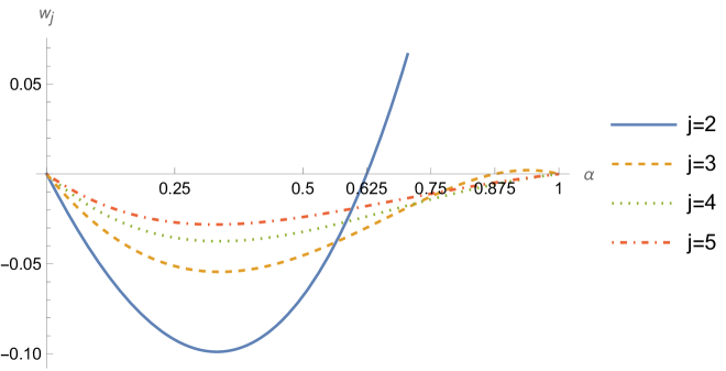
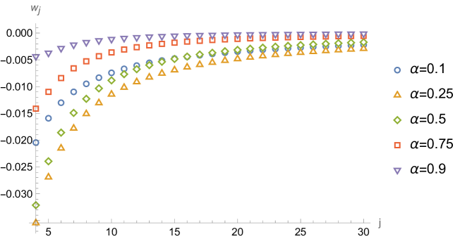
and hence, the first weight is negative, the second one only for $0<\alpha<5/8=0.625$, while the third one for $0<\alpha<7/8=0.875$. We have numerically checked the sign of a number of subsequent weights and it confirmed that all of them satisfy our assumption (A). That is to say, all BDF2 weights are admissible for $0<\alpha<5/8$. This can also be visualized numerically. In Fig. 1 we have plotted the respective weights $w_{j}$ for all $0<\alpha<1$. Computations confirm that $|w_{j}|$ are also $j-$decreasing, as can be seen in Fig. 2. It can be seen that the numerical calculations confirm our hypothesis.

Figure 1: Plot of the BDF(2) weights $w_{j}$ as in (18) for different $0<\alpha<1$ with $h=1$. Weight $w_{2}$ is negative for $0<\alpha<5/8$, weight $w_{3}$ is negative for $0<\alpha<7/8$, while all other weights are always negative.

Figure 2: Plot of the BDF(2) weights $w_{j}$ as in (18) for different $j\geq 4$ with $h=1$.

Remark 1.

We note that obtaining exact explicit formulas for the weights for the general CQ quadratures can be impossible, but only proving that they have a sign satisfying (A). However, according to the general theory of CQ we have the following (see [32], Theorem 2.1)

$$h^{-1}w_{j}=\frac{1}{\Gamma(1-\alpha)}\frac{d}{dt}t^{-\alpha}|_{t=t_{j}}+O(h^{p})=-\frac{\alpha}{\Gamma(1-\alpha)}t_{j}^{-\alpha-1}+O(h^{p}),$$ (19)

for $p\geq 1$ depending on the order of the CQ formula. From the above we can see that for $j$ sufficiently large and $h$ small, the sign of the weights is the same as the sign of $-\alpha/\Gamma(1-\alpha)$, that is, negative. Note that this conclusion is not necessarily valid for small $j$ which is precisely the case for BDF2 weights.

Going back to the general case, by the very construction of the approximation to $\partial_{t}^{\alpha}$ we have the consistency condition

$$\sum_{j=0}^{\infty}w_{j}=0\quad n\geq 1,$$ (20)

which follows by putting $\zeta=1$ into (8) or by requiring that any CQ scheme for the Caputo derivative is exact for constant functions (and hence, identically equals zero). From this it follows that for any $n\geq 1$ we have

$$\sum_{j=0}^{n}w_{j}=\sum_{j=0}^{\infty}w_{j}-\sum_{j=n+1}^{\infty}w_{j}\geq 0,$$ (21)

by the assumption (A) that the weights $w_{j}$ are negative for $j\geq 1$. We also have the truncation error

$$\partial_{t}^{\alpha}u(x,t_{n})=\partial_{h}^{\alpha}u(x,t_{n})+\zeta_{n}(h).$$ (22)

The term $\zeta_{n}(h)$ can be estimated with the help of [32], Theorem 2.2. Under the assumption that the solution has the typical regularity near the origin, that is $\|u(t)\|\leq Ct^{\alpha}$ we have

$$\|\zeta_{n}(h)\|\leq C\begin{cases}t_{n}^{-1}h,&p=1,\\ t_{n}^{-\alpha-1}h^{\alpha+1},&p\geq 2.\end{cases}$$ (23)

This clearly states how the error deteriorates near the origin due to the lack of smoothness of the solution.

We will now prove two auxiliary results that are discrete generalizations of known continuous inequalities for the Caputo derivative. They will be used later in the following section, but they are also interesting on their own. First, it is clear that the first ordinary derivative satisfies $\frac{1}{2}\frac{d}{dt}y(t)^{2}=y(t)\frac{dy}{dt}$. For the continuous Caputo derivative, it becomes an inequality $\frac{1}{2}D^{\alpha}y(t)^{2}\leq y(t)D^{\alpha}y(t)$ which is very useful when applied in the energy method (see [3, 46, 20] for recent proofs in the case where $y=y(t)\in L^{2}$ is a time-dependent mapping from the Hilbert space). As the following proposition states, this inequality is still valid for the convolution quadrature constructed above (the L1 scheme version has recently been proved in [24]).

Proposition 2.

Let the weights $w_{j}$ for the convolution quadrature (8) satisfy (A). Then, for any sequence of functions $(y^{n})_{n}\subseteq L^{2}$ with $y(0)=0$ we have

$$\frac{1}{2}\partial_{h}^{\alpha}\|y^{n}\|^{2}\leq\|y^{n}\|(\partial_{h}^{\alpha}\|y^{n}\|)\leq(\partial_{h}^{\alpha}y^{n},y^{n}).$$ (24)

Proof.

By using the definition of weights (8) we can write

$$(\partial_{h}^{\alpha}y^{n},y^{n})=w_{0}\|y^{n}\|^{2}+\sum_{j=1}^{n-1}w_{j}(y^{j},y^{n}).$$ (25)

Since by assumption (A) the negativity of $w_{j}$ for $j\geq 1$ holds, we can use the Cauchy-Schwarz inequality to obtain

$$(\partial_{h}^{\alpha}y^{n},y^{n})\geq w_{0}\|y^{n}\|^{2}+\|y^{n}\|\sum_{j=1}^{n-1}w_{j}\|y^{j}\|=\|y^{n}\|(\partial_{h}^{\alpha}\|y^{n}\|),$$ (26)

which is the first inequality that we had to prove. Furthermore, by the Cauchy inequality $ab\leq(a^{2}+b^{2})/2$ we can estimate each product with $\|y^{n}\|$ by the sum of squares

$$\|y^{n}\|(\partial_{h}^{\alpha}\|y^{n}\|)\geq\left(w_{0}+\frac{1}{2}w_{n}+\frac{1}{2}\sum_{j=1}^{n-1}w_{j}\right)\|y^{n}\|^{2}+\frac{1}{2}\sum_{j=1}^{n-1}w_{j}\|y^{j}\|^{2},$$ (27)

or, by gathering terms into the first sum with the use of the fact that $w_{0}>0$ we obtain

$$\|y^{n}\|(\partial_{h}^{\alpha}\|y^{n}\|)\geq\frac{1}{2}\|y^{n}\|^{2}\sum_{j=0}^{n}w_{j}+\frac{1}{2}\sum_{j=0}^{n}w_{j}\|y^{j}\|^{2}.$$ (28)

But, according to the consistency (21) the first term is positive leading us to the assertion. ∎

The next result concerns the discrete Grönwall inequality for the Caputo derivative. Its version for the L1 discretization has been proved, for example, in [25, 26]. The proof is based on two steps: first, we invert the derivative and then use the following classical lemma, which is a generalization of the discrete integral Grönwall inequality.

Proposition 3 (Discrete fractional Grönwall inequality (integral version) ([11], Theorem 2.1)).

Let $(y^{n})_{n}$ be a positive sequence satisfying

$$y^{n}\leq M_{0}t_{n}^{\alpha-1}+M_{1}h^{\alpha}\sum_{k=0}^{n-1}(n-k)^{\alpha-1}y^{k}+M_{2},$$ (29)

for some positive constants $M_{1,2,3}$, which may depend on $h$. Then, for $0<\alpha<1$ we have

$$y^{n}\leq M_{0}\Gamma(\alpha)t_{n}^{\alpha-1}E_{\alpha,\alpha}(M_{1}\Gamma(\alpha)t_{n}^{\alpha})+M_{2}E_{\alpha}(M_{1}\Gamma(\alpha)t_{n}^{\alpha}),$$ (30)

where the Mittag-Leffler function is defined by

$$E_{\alpha,\beta}(z)=\sum_{k=0}^{\infty}\frac{z^{k}}{\Gamma(\alpha k+\beta)},\quad E_{\alpha}:=E_{\alpha,1}.$$ (31)

Now, we can proceed to our result.

Lemma 1 (Discrete Grönwall inequality for the convolution quadrature).

Let $(y^{j})_{j=0}^{\infty}$ and $(F^{j})_{j=0}^{\infty}$ be positive sequences of numbers such that there exist $F(h)>0$ bounding the discrete fractional integral of $F$, that is,

$$h^{\alpha}\sum_{j=0}^{n-1}(n-j)^{\alpha-1}F^{j+1}\leq A(h)+B(h)t_{n}^{\alpha-1},\quad n\geq 1.$$ (32)

Assume that $y(0)=0$ and the discrete Caputo derivative $\partial_{h}^{\alpha}$ is constructed as the convolution quadrature (8) with weights that satisfy (A). Then, the inequality

$$\partial_{h}^{\alpha}y^{n}\leq\lambda_{0}y^{n}+\lambda_{1}y^{n-1}+F^{n},\quad\lambda\geq 0,$$ (33)

implies that there exists a constant $C(\alpha,\lambda_{0,1},T)>0$ and a time-step $h_{0}>0$ such that

$$y^{n}\leq C(\alpha,\lambda_{0,1},T)(A(h)+B(h)t_{n}^{\alpha-1})$$ (34)

for all $0<h\leq h_{0}<1$. For $\lambda_{0}=0$ the above is valid without any restriction on the time step $h$.

Proof.

The proof proceeds by mathematical induction. First, we will show that

$$y^{n}\leq\sum_{j=1}^{n}b_{n-j}\left(\lambda_{0}y^{j}+\lambda_{1}y^{j-1}+F^{j}\right),$$ (35)

where $b_{j}$ is defined as the CQ weight for the fractional integral (3) with the same symbol as in (8), that is

$$I^{\alpha}y(t_{n})\approx\sum_{j=0}^{n}b_{n-j}y(t_{k}),\quad\sum_{j=0}^{\infty}b_{j}\zeta^{n}=\left(\frac{\delta(\zeta)}{h}\right)^{-\alpha}$$ (36)

For $n=1$ from (8) and (A) we have

$$y^{1}\leq\frac{1}{w_{0}}\left(\lambda_{0}y^{1}+F^{1}\right),$$ (37)

but $w_{0}=-w_{1}=h^{-\alpha}\delta(0)^{-\alpha}=b_{0}^{-1}$ and, hence, $y^{1}\leq\lambda_{0}b_{0}y^{1}+b_{0}F^{1}$. This proves the initial step. Next, for convenience, set $a^{j}:=\lambda_{0}y^{j}+\lambda_{1}y^{j-1}+F^{j}$. We then assume that (35) holds for $j=1,...,n-1$. Then, by the definition of the quadrature (8) and our assumption (33) we have

$$y^{n}\leq\frac{1}{w_{0}}\left(-\sum_{j=1}^{n-1}w_{n-j}y^{j}+a^{n}\right).$$ (38)

Since $w_{j}<0$ for $j\geq 1$, the inductive assumption then gives

$$y^{n}\leq\frac{1}{w_{0}}\left(-\sum_{j=1}^{n-1}\sum_{k=1}^{j}w_{n-j}b_{j-k}a^{k}+a^{n}\right),$$ (39)

or, by changing the order of summation,

$$y^{n}\leq\frac{1}{w_{0}}\left(-\sum_{k=1}^{n-1}\left(\sum_{j=k}^{n-1}w_{n-j}b_{j-k}\right)a^{k}+a^{n}\right),$$ (40)

and we can focus on the resulting double sum. If we change the variable to $i=n-j$ we can write

$$\sum_{j=k}^{n-1}w_{n-j}b_{j-k}=\sum_{i=1}^{n-k}w_{i}b_{n-k-i}.$$ (41)

The series above can be computed using generating functions. To see this, consider the following Cauchy product of power series

$$1=\left(\frac{\delta(\zeta)}{h}\right)^{\alpha}\left(\frac{\delta(\zeta)}{h}\right)^{-\alpha}=\left(\sum_{m=0}^{\infty}w_{m}\zeta^{m}\right)\left(\sum_{m=0}^{\infty}b_{m}\zeta^{m}\right)=\sum_{m=0}^{\infty}\left(\sum_{i=0}^{m}w_{i}b_{m-i}\right)\zeta^{m}.$$ (42)

Therefore, when $m>0$ the coefficients of the rightmost power series vanish, leading to

$$-\sum_{i=1}^{n-k}w_{i}b_{n-k-i}=w_{0}b_{n-k},$$ (43)

hence,

$$y^{n}\leq\sum_{k=1}^{n-1}b_{n-k}a^{k}+\frac{1}{w_{0}}a^{n}.$$ (44)

An observation that $w_{0}=b_{0}^{-1}$ finishes the inductive step, and we have proved (35).

To proceed further we will use the fact known from the convolution quadrature theory that the weights $b_{j}$ approximate the continuous kernel, that is (see for example [32], formula (2.6))

$$|b_{0}|\leq Ch^{\alpha-1},\quad|b_{j}|\leq Ch(jh)^{\alpha-1}=Ch^{\alpha}j^{\alpha-1},\quad j\geq 1,$$ (45)

for some constant $C=C(\alpha)$. Therefore, separating the last term in the sum (35) yields

$$\begin{split}y^{n}&\leq C(\alpha)h^{\alpha}\left(\lambda_{0}y^{n}+\lambda_{0}\sum_{j=1}^{n-1}(n-j)^{\alpha-1}y^{j}+\lambda_{1}y^{n-1}+\lambda_{1}\sum_{j=1}^{n-1}(n-j)^{\alpha-1}y^{j-1}\right.\\ &\left.+F^{n}+\sum_{j=1}^{n-1}(n-j)^{\alpha-1}F^{j}\right).\end{split}$$ (46)

All terms involving $y^{j}$ for $j\leq n-1$ can be estimated by a common sum. To see this observe that in the sum of $y^{j-1}$ we can change the summation variable $j-1\mapsto j$ and use the elementary inequality

$$(n-j-1)^{\alpha-1}\leq 2^{1-\alpha}(n-j)^{\alpha-1},\quad\mbox{for}\quad 0\leq j\leq n-2,$$ (47)

to obtain

$$\begin{split}\lambda_{0}&\sum_{j=1}^{n-1}(n-j)^{\alpha-1}y^{j}+\lambda_{1}y^{n-1}+\lambda_{1}\sum_{j=0}^{n-2}(n-j-1)^{\alpha-1}y^{j}\\ &\leq\lambda_{0}\sum_{j=1}^{n-1}(n-j)^{\alpha-1}y^{j}+\lambda_{1}y^{n-1}+2^{1-\alpha}\lambda_{1}\sum_{j=0}^{n-2}(n-j)^{\alpha-1}y^{j}\leq(\lambda_{0}+2^{1-\alpha}\lambda_{1})\sum_{j=0}^{n-1}(n-j)^{\alpha-1}y^{j}\end{split}$$ (48)

Next, fix any time-step $h_{0}>0$ for which $1-C(\alpha)\lambda_{0}h_{0}^{\alpha}>0$. Then, for $0<h\leq h_{0}$ we can factor out $y^{n}$,

$$y^{n}\leq\frac{C(\alpha)(\lambda_{0}+2^{1-\alpha}\lambda_{1})}{1-C(\alpha)\lambda_{0}h_{0}^{\alpha}}h^{\alpha}\sum_{j=0}^{n-1}(n-j)^{\alpha-1}y^{j}+\frac{C(\alpha)2^{1-\alpha}}{1-C(\alpha)\lambda_{0}h_{0}^{\alpha}}h^{\alpha}\sum_{j=1}^{n}(n-j+1)^{\alpha-1}F^{j},$$ (49)

where we have used again (47), with the index shifted by one, in the sum with $F^{j}$. This can be further estimated with the use of the assumption of bounded fractional integral of $F^{n}$, that is, using (32) we obtain (after changing the summation variable $j\mapsto j+1$)

$$y^{n}\leq\frac{C(\alpha)(\lambda_{0}+2^{1-\alpha}\lambda_{1})}{1-C(\alpha)\lambda_{0}h_{0}^{\alpha}}\sum_{j=0}^{n-1}(n-j)^{\alpha-1}y^{j}+\frac{C(\alpha)2^{1-\alpha}}{1-C(\alpha)\lambda_{0}h_{0}^{\alpha}}(A(h)+B(h)t_{n}^{\alpha-1}).$$ (50)

Set $M=C(\alpha)/(1-C(\alpha)\lambda_{0}h_{0}^{\alpha})$. We can now invoke Proposition 3 with $M_{0}=B(h)M2^{1-\alpha}$ , $M_{1}=(\lambda_{0}+2^{1-\alpha}\lambda_{1})M$, and $M_{2}=A(h)M2^{1-\alpha}$, to obtain

$$y^{n}\leq M\Gamma(\alpha)E_{\alpha,\alpha}(M_{1}\Gamma(\alpha)t_{n}^{\alpha})t_{n}^{\alpha-1}B(h)+ME_{\alpha}\left(M_{1}\Gamma(\alpha)t_{n}^{\alpha}\right)A(h).$$ (51)

Finally, we have $t_{n}\leq T$ and after redefinition of the constant $C(\alpha,\lambda_{0,1},T)$ we arrive at the conclusion. ∎

3 Fully discrete scheme for the quasilinear subdiffusion equation

We can now proceed to the derivation of the fully discrete scheme to solve (1). Take any test function $\chi\in H^{1}(\Omega)$, then by integrating by parts, we can obtain the following

$$(\partial^{\alpha}_{t}u,\chi)+a(D(t,u);u,\chi)=(f(t,u),\chi),\quad\chi\in H^{1}(\Omega),$$ (52)

with $u(0)=\varphi$. Here, we defined the form

$$a(w;u,v):=\int_{\Omega}w(x)\nabla u\nabla vdx.$$ (53)

To discretize the above in time, we use the convolution quadrature (8) for the Caputo derivative and the finite element method (FEM) for the spatial variables. Let $\mathcal{T}_{h}$ be the family of shape-regular quasi-uniform triangulations of $\overline{\Omega}$ with the maximal diameter $k=\max_{K\in\mathcal{T}_{k}}\text{diam}K$. By $V_{k}\subset H_{0}^{1}(\Omega)$ denote the standard continuous piecewise linear function space over $\mathcal{T}_{k}$ that vanish on the boundary $\partial\Omega$

$$V_{k}:=\left\{\chi_{k}\in C^{0}(\overline{\Omega}):\;\chi_{k}|_{K}\text{ is linear for all }K\in\mathcal{T}_{k}\text{ and }\chi_{k}|_{\partial\Omega}=0\right\}.$$ (54)

Therefore, denoting by $U^{n}\in V_{k}$ the numerical approximation of $u(t_{n})$ we devise the semi-implicit scheme

$$\begin{cases}(\partial_{h}^{\alpha}U^{n},\chi)+a(D(t_{n},U^{n-1});U^{n},\chi)=(f(t_{n},U^{n-1}),\chi),&\chi\in V_{k},\;n\geq 1,\\ U^{0}=0,&\\ \end{cases}$$ (55)

In what follows, we will utilize some notions of projecting a function on a finite-dimensional space. For example, we can use the orthogonal projection $P_{k}$ defined as

$$(P_{k}u-u,\chi)=0,\quad\chi\in V_{k},$$ (56)

or the Ritz elliptic projection $R_{k}$ for fixed $0\leq t\leq T$

$$a(D(t,u);R_{k}u(t)-u(t),\chi)=0,\quad\chi\in V_{k}.$$ (57)

The latter is particularly useful in the convergence proof. Observe that to find $R_{n}u(t)$ it is necessary to solve a linear elliptic problem. From the general theory of PDEs we know the error estimates on these projections when $u\in C([0,T];H^{m}(\Omega))$ [44, 33]

$$\|u-P_{k}u\|_{p}\leq Ck^{m-p}\|u\|_{m},\quad\|u-R_{k}u\|_{p}\leq Ck^{m-p}\|u\|_{m},\quad\|(u-R_{k}u)_{t}\|_{p}\leq Ck^{m-p}\|u\|_{m}$$ (58)

Moreover, for $u\in L^{\infty}(\Omega)$ we have

$$\|R_{k}u\|_{\infty}\leq C.$$ (59)

Finally, note also that in all nonlinearities of the equation, that is, $D$ and $f$, the time step has been delayed by one in order to obtain a fully linear scheme for the solution to the nonlinear equation. Having the results from the previous section, it is straightforward to prove that the scheme is stable.

Proposition 4 (Stability).

Let $U^{n}$ be the solution of (55). Suppose that there exists a function $g=g(t)$ such that $\|f(t,u)\|\leq g(t)$ with $I^{\alpha}g(t)\leq F$. Then, we have

$$\|U^{n}\|\leq C(\alpha,T)F.$$ (60)

Proof.

Let $\chi=U^{n}\in V_{k}$ in (55), then from the Proposition 2 and the Cauchy inequality 2 we have

$$\|U^{n}\|(\partial_{h}^{\alpha}\|U^{n}\|)+a(D(t,U^{n-1}),U^{n},U^{n})\leq\|U^{n}\|g(t_{n}).$$ (61)

Since, by definition (53) the $a$-form is positive-definite we further have

$$\|U^{n}\|(\partial_{h}^{\alpha}\|U^{n}\|)\leq\|U^{n}\|g(t_{n}),$$ (62)

or

$$\partial_{h}^{\alpha}\|U^{n}\|\leq g(t_{n}).$$ (63)

Now, notice that there exists a constant $C$ such that

$$h^{\alpha}\sum_{j=0}^{n-1}(n-j)^{\alpha-1}g(t_{j})\leq CI^{\alpha}g(t_{n})\leq CF,$$ (64)

since the rectangle discretization of the fractional integral converges to the continuous one. The application of Lemma 1 ends the proof. ∎

Now, we can proceed to the convergence proof. As mentioned in the Introduction, the regularity assumption on the solution is the typical for the subdiffusion equation. Due to the lack of relevant results in the literature for quasilinear equations, we have to put this regularity requirement as an assumption. Investigating this issue further is the subject of our future work.

Theorem 1 (Convergence).

Let $U^{n}$ be the solution of the scheme (55) as a numerical approximation at $t=t_{n}$ to the solution $u$ of (1). Assume that for all $t,s\in[0,T]$ the solution satisfies the assumption of time regularity (7) and is $H_{0}^{1}(\Omega)\cap H^{2}(\Omega)$ in space. Then, for sufficiently small $h>0$ we have

$$\|u(t_{n})-U^{n}\|\leq C(\alpha,T,u)\left(A(h)+(h^{2-\alpha}+B(h))t_{n}^{\alpha-1}+k^{2}\right),$$ (65)

where $A(h)$ and $B(h)$ satisfy

$$h^{\alpha}\sum_{j=0}^{n-1}(n-j)^{\alpha-1}\|\zeta_{j+1}(h)\|\leq A(h)+B(h)t_{n}^{\alpha-1}.$$ (66)

and $\zeta_{j+1}(h)$ is the truncation error (22) for the convolution quadrature for the Caputo derivative defined in (8) with assumptions (A).

Proof.

We will start by writing the error equation for the problem. Set in a standard way $e^{n}:=u(t_{n})-U^{n}=u(t_{n})-R_{k}u(t_{n})+R_{k}u(t_{n})-U^{n}=:\rho^{n}+\theta^{n}$. The decomposition of $e^{n}$ into $\rho^{n}$ and $\theta^{n}$ is very useful since the estimate on $\rho^{n}$ follows from general theory (58) while $\theta^{n}$ belongs to the finite-dimensional space $V_{k}$. Therefore, it is sufficient to find a bound on the latter error. Hence, observe that for any $\chi\in V_{k}$ from the definition of error decomposition into $\rho^{n}$ and $\theta^{n}$ we have

$$\begin{split}(\partial_{h}^{\alpha}&\theta^{n},\chi)+a(D(t_{n},U^{n-1});\theta^{n},\chi)\\ &\stackrel{{\scriptstyle\text{def. of }\theta^{n}}}{{=}}(\partial_{h}^{\alpha}R_{k}u(t_{n}),\chi)-(\partial_{h}^{\alpha}U^{n},\chi))+a(D(t_{n},U^{n-1});R_{k}u(t_{n}),\chi)-a(D(t_{n},U^{n-1});U^{n},\chi).\end{split}$$ (67)

Now, using the numerical scheme (55) we can identify the source term

$$\begin{split}(\partial_{h}^{\alpha}&\theta^{n},\chi)+a(D(t_{n},U^{n-1});\theta^{n},\chi)\\ &\stackrel{{\scriptstyle\eqref{eqn:NumericalScheme}}}{{=}}(\partial_{h}^{\alpha}R_{k}u(t_{n}),\chi)+a(D(t_{n},U^{n-1});R_{k}u(t_{n}),\chi)-(f(t_{n},U^{n-1}),\chi).\end{split}$$ (68)

Next, the definition of $\rho^{n}$ and the PDE itself (52) leads to

$$\begin{split}(\partial_{h}^{\alpha}\theta^{n},\chi)+&a(D(t_{n},U^{n-1});\theta^{n},\chi)\stackrel{{\scriptstyle\text{def. of }\rho^{n}}}{{=}}-(\partial_{h}^{\alpha}\rho^{n},\chi)+((\partial_{h}^{\alpha}-\partial_{t}^{\alpha})u(t_{n}),\chi)+(\partial_{t}^{\alpha}u(t_{n}),\chi)\\ &+a(D(t_{n},U^{n-1});R_{k}u(t_{n}),\chi)-(f(t_{n},U^{n-1}),\chi)\\ &\stackrel{{\scriptstyle\eqref{eqn:MainPDEWeak}}}{{=}}-(\partial_{h}^{\alpha}\rho^{n},\chi)+((\partial_{h}^{\alpha}-\partial_{t}^{\alpha})u(t_{n}),\chi)-a(D(t_{n},u(t_{n}));u(t_{n}),\chi)+a(D(t_{n},U^{n-1});R_{k}u(t_{n}),\chi)\\ &+(f(t_{n},u(t_{n}))-f(t_{n},U^{n-1}),\chi).\end{split}$$ (69)

Now, we can use the definition of the Ritz projection (57) to write $R_{k}u$ instead of $u$ in the $a$-form

$$\begin{split}(\partial_{h}^{\alpha}\theta^{n},\chi)&+a(D(t_{n},U^{n-1});\theta^{n},\chi)=-(\partial_{h}^{\alpha}\rho^{n},\chi)+((\partial_{h}^{\alpha}-\partial_{t}^{\alpha})u(t_{n}),\chi)\\ &+a(D(t_{n},U^{n-1})-D(t_{n},u(t_{n}));R_{k}u(t_{n}),\chi)+(f(t_{n},u(t_{n}))-f(t_{n},U^{n-1}),\chi).\end{split}$$ (70)

We see that the right hand side in the equation for the error $\theta^{n}$ above decomposes into four terms:

1. Ritz projection error,

2. truncation error of the Caputo derivative,

3. nonlinearity of the diffusivity,

4. nonlinearity of the source.

Therefore, by setting $\chi=\theta^{n}\in V_{k}$ we can obtain

$$\begin{split}(\partial_{h}^{\alpha}\theta^{n},\theta^{n})&+a(D(t_{n},U^{n-1});\theta^{n},\theta^{n})\leq\|\partial_{h}^{\alpha}\rho^{n}\|\|\theta^{n}\|+|(\partial_{h}^{\alpha}-\partial_{t}^{\alpha})u(t_{n})\|\|\theta^{n}\|\\ &+|a(D(t_{n},U^{n-1})-D(t_{n},u(t_{n}));R_{k}u(t_{n}),\theta^{n})|+L\|u(t_{n})-U^{n-1}\|\|\theta^{n}\|,\end{split}$$ (71)

where we have used the assumption of Lipschitz continuity of $f$ as in (4). Now, from the definition of the $a$-form (53) we can further estimate

$$\begin{split}|a(D(t_{n},U^{n-1})&-D(t_{n},u(t_{n}));R_{k}u(t_{n}),\theta^{n})|\leq\int_{\Omega}|D(t_{n},U^{n-1})-D(t_{n},u(t_{n}))||\nabla R_{k}u(t_{n})||\nabla\theta^{n}|dx\\ &\leq C(u)\|R_{k}u(t_{n})\|_{\infty}\int_{\Omega}|D(t_{n},U^{n-1})-D(t_{n},u(t_{n}))||\nabla\theta^{n}|dx\\ &\leq C(u)\|U^{n-1}-u(t_{n})\|\|\nabla\theta^{n}\|,\end{split}$$ (72)

where we have used (59) and the Lipschitz continuity of $D$ and Schwartz inequality. Now, since by (4) we have $D(x,t,u)\geq D_{-}$, it follows that

$$(\partial_{h}^{\alpha}\theta^{n},\theta^{n})+D_{-}\|\nabla\theta^{n}\|^{2}\leq\|\partial_{h}^{\alpha}\rho^{n}\|\|\theta^{n}\|+C(u)\left(|\zeta_{n}(h)|\|\theta^{n}\|+\|U^{n-1}-u(t_{n})\|\left(\|\nabla\theta^{n}\|+\|\theta^{n}\|\right)\right),$$ (73)

where we have explicitly written down the truncation error (22) for the quadrature. The next step is to bound the difference of solutions at a retarded time

$$\|U^{n-1}-u(t_{n})\|\leq\|U^{n-1}-u(t_{n-1})\|+\|u(t_{n-1})-u(t_{n})\|\leq\|\rho^{n-1}\|+\|\theta^{n-1}\|+\|u(t_{n-1})-u(t_{n})\|.$$ (74)

Due to the assumed temporal regularity (7) we have

$$\|u(t_{n-1})-u(t_{n})\|\leq C(u)t_{n}^{\alpha-1}h,\quad n\geq 1,$$ (75)

whence,

$$\begin{split}(\partial_{h}^{\alpha}\theta^{n},\theta^{n})+D_{-}\|\nabla\theta^{n}\|^{2}&\leq\|\partial_{h}^{\alpha}\rho^{n}\|\|\theta^{n}\|+\\ &C(u)\left(|\zeta_{n}(h)|\|\theta^{n}\|+\left(\|\rho^{n-1}\|+\|\theta^{n-1}\|+t_{n}^{\alpha-1}h\right)\left(\|\nabla\theta^{n}\|+\|\theta^{n}\|\right)\right).\end{split}$$ (76)

By using Poincaré-Friedrichs inequality we can write $\|\theta^{n}\|\leq C\|\nabla\theta^{n}\|$ and factor out the norm of the gradient

$$(\partial_{h}^{\alpha}\theta^{n},\theta^{n})+D_{-}\|\nabla\theta^{n}\|^{2}\leq C(u)\left(\|\partial_{h}^{\alpha}\rho^{n}\|+|\zeta_{n}(h)|+\|\rho^{n-1}\|+\|\theta^{n-1}\|+t_{n}^{\alpha-1}h\right)\|\nabla\theta^{n}\|.$$ (77)

Furthermore, we can use the $\epsilon$-Cauchy inequality $ab\leq\frac{\epsilon}{2}a^{2}+\frac{1}{2\epsilon}b^{2}$, with an appropriate choice of $\epsilon$ to cancel the gradient term

$$(\partial_{h}^{\alpha}\theta^{n},\theta^{n})+D_{-}\|\nabla\theta^{n}\|^{2}\leq C(u)\left(\|\partial_{h}^{\alpha}\rho^{n}\|+|\zeta_{n}(h)|+\|\rho^{n-1}\|+\|\theta^{n-1}\|+t_{n}^{\alpha-1}h\right)^{2}+D_{-}\|\nabla\theta^{n}\|^{2},$$ (78)

or by using Proposition 2 and a simple inequality $(a+b)^{2}\leq 2(a^{2}+b^{2})$

$$\partial_{h}^{\alpha}\|\theta^{n}\|^{2}\leq C(u)\left(\left(\|\partial_{h}^{\alpha}\rho^{n}\|+|\zeta_{n}(h)|+\|\rho^{n-1}\|+t_{n}^{\alpha-1}h\right)^{2}+\|\theta^{n-1}\|^{2}\right).$$ (79)

The above form is almost ready for the discrete fractional Grönwall inequality (Lemma 1). Before doing that, we have to estimate the $\rho$ terms in the first inner parentheses. To this end, notice that by (58) we immediately have $\|\rho^{n}\|\leq C(u,T)k^{2}$ since $t\in[0,T]$ and $u$ is continuous on $[0,T]$. Denoting $\rho(t)=u(t)-R_{k}u(t)$, so that $\rho^{n}=\rho(t_{n})$, we can bound

$$\begin{split}\|\partial_{h}^{\alpha}\rho^{n}\|&\leq\|(\partial_{h}^{\alpha}-\partial^{\alpha}_{t})\rho(t_{n})\|+\|\partial_{t}^{\alpha}\rho(t_{n})\|\leq|\zeta_{n}(h)|+\frac{1}{\Gamma(1-\alpha)}\int_{0}^{t_{n}}(t_{n}-s)^{-\alpha}\|(u-R_{k}u)_{t}(s)\|ds\\ &\leq|\zeta_{n}(h)|+C(u)\frac{k^{2}}{\Gamma(1-\alpha)}\int_{0}^{t_{n}}(t_{n}-s)^{-\alpha}ds=|\zeta_{n}(h)|+C(u)k^{2}\frac{t_{n}^{1-\alpha}}{\Gamma(2-\alpha)}\\ &\leq|\zeta_{n}(h)|+C(\alpha,T,u)k^{2}.\end{split}$$ (80)

Whence,

$$\partial_{h}^{\alpha}\|\theta^{n}\|^{2}\leq C(\alpha,T,u)\left(\left(|\zeta_{n}(h)|+t_{n}^{\alpha-1}h+k^{2}\right)^{2}+\|\theta^{n-1}\|^{2}\right).$$ (81)

Now, by invoking Lemma 1 and using some elementary estimates on $(a+b)^{2}$ we obtain

$$\|\theta^{n}\|^{2}\leq C(\alpha,T,u)\left(\left(A(h)+B(h)t_{n}^{\alpha-1}+E(h)+k^{2}\right)^{2}\right),$$ (82)

where $A(h)$, and $B(h)$ are defined in (66) and the quantity $E(h)$ is

$$\begin{split}E(h)&=h^{2\alpha}\sum_{j=0}^{n-1}(n-j)^{\alpha-1}(j+1)^{\alpha-1}=h^{2\alpha}n^{2\alpha-1}\frac{1}{2}\sum_{j=0}^{n-1}\left(1-\frac{j}{n}\right)^{\alpha-1}\left(\frac{j}{n}+\frac{1}{n}\right)^{\alpha-1}\\ &\leq Ch^{2\alpha}n^{2\alpha-1}\int_{0}^{1}(1-x)^{\alpha-1}x^{\alpha-1}dx=Ct_{n}t_{n}^{\alpha-1}h\leq CTt_{n}^{\alpha-1}h.\end{split}$$ (83)

Finally, by definition we have $\theta^{0}=R_{k}u(0)-U^{0}=0$ since our initial condition vanishes, and this brings us to

$$\|\theta^{n}\|^{2}\leq C(\alpha,T,u)\left(A(h)+B(h)t_{n}^{\alpha-1}+t_{n}^{\alpha-1}h+k^{2}\right)^{2},$$ (84)

and the proof is complete. ∎

For the BDF$(p)$ CQ of the order $p\geq 1$ we can infer the exact order of the convergence of our numerical scheme.

Corollary 1.

Let the assumptions of Theorem 1 be satisfied. Then, when the Caputo derivative is discretized with the BDF$(p)$ CQ we have the following

$$\|u(t_{n})-U^{n}\|\leq C(\alpha,T,u)\begin{cases}t_{n}^{\alpha-1}h\ln h^{-1}+k^{2},&p=1,\\ t_{n}^{\alpha-1}h+k^{2},&p\geq 2,\\ \end{cases}$$ (85)

for $n$ large enough and sufficiently small $h$.

Proof.

To prove the assertion, we have to find out the form of $A(h)$ and $B(h)$ defined in Theorem 1. They come from the bound of the discrete fractional integral of $\zeta_{n}(h)$, that is, the truncation error of the Caputo derivative as in (22). First, assume that $p=1$, that is, we consider the Euler scheme. From (23) we have

$$h^{\alpha}\sum_{j=0}^{n-1}(n-j)^{\alpha-1}\|\zeta_{j+1}(h)\|\leq Ch^{\alpha}\sum_{j=0}^{n-1}(n-j)^{\alpha-1}(j+1)^{-1}\leq Ch^{\alpha}n^{\alpha-1}\frac{1}{n}\sum_{j=1}^{n}\left(1+\frac{1}{n}-\frac{j}{n}\right)^{\alpha-1}\left(\frac{j}{n}\right)^{-1},$$ (86)

where we have changed the summation order via $j\mapsto j-1$. As can be seen, the resulting expression is the Riemann sum of a convergent integral, hence with a suitable choice of the constant

$$h^{\alpha}\sum_{j=0}^{n-1}(n-j)^{\alpha-1}\|\zeta_{j+1}(h)\|\leq Ch^{\alpha}n^{\alpha-1}\int_{\frac{1}{n}}^{1}(1-x)^{\alpha-1}\frac{dx}{x}.$$ (87)

This integral can be evaluated exactly with the help of the hypergeometric function, but for our needs, we only have to find its leading order behavior for large $n$. To this end, for arbitrary $\frac{1}{n}<\epsilon<1$, we split the integral into two parts

$$\begin{split}\int_{\frac{1}{n}}^{1}(1-x)^{\alpha-1}\frac{dx}{x}&=\int_{\frac{1}{n}}^{\epsilon}(1-x)^{\alpha-1}\frac{dx}{x}+\int_{\epsilon}^{1}(1-x)^{\alpha-1}\frac{dx}{x}\leq(1-\epsilon)^{\alpha-1}\int_{\frac{1}{n}}^{\epsilon}\frac{dx}{x}+\frac{1}{\epsilon}\int_{\epsilon}^{1}(1-x)^{\alpha-1}dx\\ &=(1-\epsilon)^{\alpha-1}\ln\left(n\epsilon\right)+\frac{(1-\epsilon)^{\alpha}}{\epsilon\alpha}\leq C\ln n,\end{split}$$ (88)

and, hence, for sufficiently small $h>0$

$$\begin{split}h^{\alpha}\sum_{j=0}^{n-1}(n-j)^{\alpha-1}\|\zeta_{j+1}(h)\|&\leq C(nh)^{\alpha-1}h\ln n=Ct_{n}^{\alpha-1}h(\ln(nh)-\ln h)\\ &\leq Ct_{n}^{\alpha-1}h(\ln T-\ln h)\leq Ct_{n}^{\alpha-1}h\ln h^{-1}.\end{split}$$ (89)

This gives us $A(h)=0$, $B(h)=Ch\ln h^{-1}$ and proves the case with $p=1$.

Now, assume that $p\geq 2$. By a similar reasoning we can identify the Riemann sum of the corresponding integral and obtain

$$\begin{split}h^{\alpha}\sum_{j=0}^{n-1}(n-j)^{\alpha-1}\|\zeta_{j+1}(h)\|&\leq Ch^{1+\alpha}\int_{0}^{t_{n}}(t_{n}-s)^{\alpha-1}(s+h)^{-\alpha-1}ds\\ &=C(nh)^{\alpha-1}\frac{nh}{\alpha(1+n)}\leq\frac{1}{\alpha}Ct_{n}^{\alpha-1}h\end{split}$$ (90)

since the appearing integral has an exact primitive $-\frac{1}{\alpha(t_{n}+h)}\left(\frac{t_{n}-s}{h+s}\right)^{\alpha}$. This time we have $A(h)=0$ and $B(h)=Ch$. Combining the case $p\geq 2$ with (65) finishes the proof. ∎

As can be seen, the overall error for our scheme based on BDF1-CQ is equal to $t_{n}^{\alpha-1}h\ln h^{-1}+k^{2}$, which is always second order in space. For a fixed time $t_{n}>0$, that is, locally, the order in time is $1$ (apart from the logarithmic term). On the other hand, the global (maximal) error in time is of the order $\alpha$. This behavior is precisely what can be expected from the same scheme applied to the linear subdiffusion equation, due to lower regularity of the solution near the origin. However, note that our assumption (7) does not require the existence of higher derivatives as opposed to the various requirements found in the literature.

4 Fast and oblivious implementation

To implement our numerical scheme (55) , we fix a basis of the $V_{k}$ space and expand the solution $U^{n}$, that is

$$U^{n}=\sum_{k=1}^{M}y_{k}^{n}\Phi_{k}.$$ (91)

Taking $\chi=\Phi_{j}$, denoting $\textbf{y}^{n}=(y_{1}^{n},...,y_{M}^{n})$, and plugging the above into (55) we obtain the following

$$B\partial_{h}^{\alpha}\textbf{y}^{n}+A(\textbf{y}^{n-1})\textbf{y}^{n}=\textbf{f}^{n}(\textbf{y}^{n-1}),$$ (92)

where the mass matrix $B=\left\{B_{ij}\right\}_{i,j=1}^{M}$, the stiffness matrix $A=\left\{A_{ij}\right\}_{i,j=1}^{M}$, and the load vector $\textbf{f}^{n}=\left\{f_{i}^{n}\right\}_{i=1}^{M}$ are defined by

$$B_{ij}=(\Phi_{i},\Phi_{j}),\quad A_{ij}(\textbf{y}^{n-1})=a\left(D\left(\sum_{k=1}^{M}y_{k}^{n-1}\Phi_{k}\right);\Phi_{i},\Phi_{j}\right),\quad f_{i}^{n-1}=\left(f\left(t_{n},\sum_{k=1}^{M}y_{k}^{n-1}\Phi_{k}\right),\Phi_{i}\right).$$ (93)

Finally, we discretize the Caputo derivative according to the CQ scheme (8) to arrive at a linear system of algebraic equations

$$\left(w_{0}B+A(\textbf{y}^{n-1})\right)\textbf{y}^{n}=-B\sum_{j=0}^{n-1}w_{n-j}\textbf{y}^{j}+\textbf{f}^{n}(\textbf{y}^{n-1}),$$ (94)

which clearly indicates the non locality in time: the right-hand side depends on the historical values of the solution $\textbf{y}^{i}$ for $i=0,1,...,n-1$. As a simple example of the basis, in one spatial dimension we can have $\Omega=(0,1)$ for which we can take the usual tent functions

$$\Phi_{j}(x)=\begin{cases}1-\left|\dfrac{x-x_{j}}{k}\right|,&|x-x_{j}|\leq k,\\ 0,&|x-x_{j}|>k.\\ \end{cases}$$ (95)

However, we do not directly implement (94). Instead, we apply the fast algorithm developed in [5] for the evaluation of the fractional integral, in order to deal with memory more efficiently and reduce computational cost. To do this, we use the preservation of the composition rule by all CQ schemes, which implies

$$\partial_{h}^{\alpha}\textbf{y}^{n}=\partial_{h}^{\alpha-1}\partial_{h}^{1}\textbf{y}^{n}.$$

In the case of the Euler based CQ, this yields

$$\partial_{h}^{\alpha}\textbf{y}^{n}=\partial_{h}^{\alpha-1}\textbf{v}^{n},\quad\mbox{with }\quad\textbf{v}^{n}:=\frac{\textbf{y}^{n}-\textbf{y}^{n-1}}{h}.$$

Setting $\widetilde{\omega}_{j}$ the Euler based CQ weights associated with the fractional integral $\partial_{h}^{\alpha-1}$, for $j=0,\dots,N$, we obtain from (8)

$$B\sum_{j=0}^{n}\widetilde{\omega}_{n-j}\textbf{v}_{j}+A(\textbf{y}^{n-1})\textbf{y}^{n}=\textbf{f}^{n}(\textbf{y}^{n-1}),$$ (96)

which leads to the linear system

$$\left(\frac{1}{h}B\widetilde{\omega}_{0}+A(\textbf{y}^{n-1})\right)\textbf{y}^{n}=\frac{1}{h}\widetilde{\omega}_{0}B\textbf{y}^{n-1}+\textbf{f}^{n}(\textbf{y}^{n-1})-B\sum_{j=0}^{n-1}\widetilde{\omega}_{n-j}\textbf{v}_{j}.$$ (97)

The computation of the memory term on the right-hand side requires in principle the precomputation and storage of all the CQ weights $\widetilde{\omega}_{j}$, $j=0,\dots,N$, the storage of all vectors $\textbf{v}_{j}$, with $j=0,\dots,n-1$, and $2n$ operations per time step, implying a total complexity growing like $O(N^{2})$, as $N\to\infty$. The algorithm in [5] uses a special integral representation and quadrature to compute the CQ weights within a prescribed precision $\varepsilon$ and manages to reduce the complexity to $O(N\log{N}\log(\frac{1}{\varepsilon}))$. Moreover, if we are only interested in the solution at the final time $T$, the memory in the evaluation of the right-hand side grows like $O(\log{N}\log(\frac{1}{\varepsilon}))$, since the algorithm does not need to store the entire history $\textbf{v}_{j}$, for all $j<n$, and all the CQ weights. Instead, for a moderate value of $n_{0}$, such as $n_{0}=4,5$, only the first $n_{0}+1$ CQ weights $\widetilde{\omega}_{j}$ and the last $n_{0}+2$ values of $\textbf{v}_{n-j}$, with $0\leq j\leq n_{0}+2$, are required in storage, together with $O(\log{N}\log(\frac{1}{\varepsilon}))$ linear combinations of the history $\textbf{v}_{n-j}$, with $j>n_{0}+1$. Although the main part of the computational cost of the method (97) lays in the assembly of the stiffness matrix $A(\textbf{y}^{n-1})$ at every time step, we can see from the results reported in the next Section that the application of the algorithm in [5] is advantageous from the complexity point of view. CPU times are globally reduced by a factor of almost two, as shown in Figure 4. Since in the present paper we are mostly interested in the verification of our error estimates, both pointwise and uniform in time, we compute and store the numerical solution $y^{n}$ for every $1\leq n\leq N$ and do not use an oblivious version of the algorithm.

5 Numerical examples

We will illustrate our results with some numerical examples. For illustration purposes, we take $\Omega=(0,1)$ as our spatial domain and focus only on the temporal features of the solved solution. The discretization in space has been implemented as the finite element method described in the previous section. The grid has been taken to be sufficiently fine to be able to neglect all errors of spatial nature when compared to temporal discretization. The discretization of the fractional derivative is done using Euler based CQ since, due to low regularity of the solution, higher-order methods do not have any advantage over this one.

We consider two exemplary problems: one will be chosen artificially in order to have an exact solution

$$\begin{split}D(x,t,u)&=1+u,\quad f(x,t,u)=\pi^{2}\left(u+2u^{2}-t^{2\alpha}\right)+\Gamma(1+\alpha)\sin(\pi x),\\ u(x,t)&=t^{\alpha}\sin(\pi x),\end{split}$$ (98)

which models the typical solution’s behavior at $t=0$. The second example is a more realistic model of a porous medium with exponential diffusivity and a simple concentrated source. The diffusivity in porous media strongly depends on the moisture content (for example, see [13]) and exponential model is one of the typical choices

$$D(x,t,u)=e^{-u},\quad f(x,t,u)=\frac{1}{\sqrt{4\pi\delta}}e^{-\frac{(x-x_{0})^{2}}{4\delta}},\quad u(x,0)=0.$$ (99)

Parameters $k$, $x_{0}$, and $\delta$ are chosen accordingly for a particular simulation. Note that in this case, we do not possess an exact analytic solution.

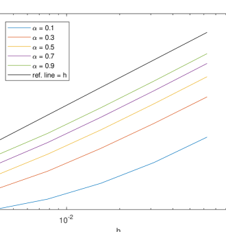
In the first example (98) we can compare the numerical solution with the exact one and compute the error at the final time of the simulation $t=T$, that is, for each $\alpha$ we find $\|u(T)-U^{n}\|$, where $nh=T$. Note, however, that this error is limited by the spatial discretization error that can be eliminated by choosing a sufficiently small grid spacing. The results of our calculations are presented in Fig. 3. As we can see, numerical computations verify that the scheme is convergent even for the nonsmooth in time case. The real order of convergence is consistent with $1$ for most values of $\alpha$, which is the order of Euler discretization. This is consistent with the results of Corollary 1 apart from the logarithmic part, which is difficult to resolve numerically and can cause certain discrepancies for small $h$. However, we can conclude that numerical simulations confirm the theoretical results.

Figure 3: Error $\|u(T)-U^{n}\|$ with $nh=T=1$ for the problem (98).

For the second example (99) the error cannot be computed directly and we will estimate the order of convergence by the Aitken extrapolation [27]. Assume that the error can be estimated with $\max_{n}\|U^{n}_{h}-U^{n}_{h/2}\|\approx Ch^{p}$, where as a reference solution we take the one computed on a twice finer grid. Then, by halving the grid once more and taking the logarithm we can write

$$p\approx\log_{2}\frac{\|U^{n}_{h}-U^{n}_{h/2}\|}{\|U^{n}_{h/2}-U^{n}_{h/4}\|},\quad\text{with fixed}\quad nh=t_{n}=T.$$ (100)

That is to say, the order is estimated based on the pointwise norm in time and the $L^{2}$ norm in space, in line with our results from previous sections. The results of our computations are gathered in Tab. 1. As we can see, the estimated order is close to $1$ for all values of $\alpha$, again consistent with the Euler discretization measured pointwise in time.

$\alpha$	0.1	0.2	0.3	0.4	0.5	0.6	0.7	0.8	0.9
order	0.77	0.90	1.06	1.08	0.93	0.93	1.03	0.93	1.11

Table 1: Estimated order of convergence for the second example (99) for different $\alpha$. The basis of our calculation has been taken $h=2^{-8}$ for the formula (100) and $T=1$.

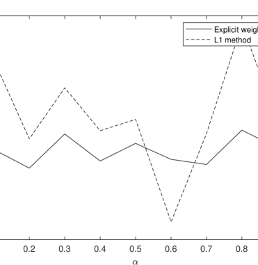
The final example concerns the temporal complexity of our algorithm. We have compared the computation times of three ways of implementing the time integration of our PDE: with and without fast and oblivious algorithm described in the previous section, and the L1 scheme. In Fig. 4 we can see the following ratio computed for different values of $\alpha$

$$\frac{\text{computation time of a standard or L1 implementation}}{\text{computation time of the fast and obliovious implementation}}.$$ (101)

The problem tested is our second example (99). In our calculations, we have taken $h=2^{-9}$ but also tested other values. Also, to obtain Fig. 4 independent of various computer background processes, we have conducted simulations $100$ times and taken the mean values. The results are uniform with respect to $\alpha$ (note the vertical scale) and indicate that the fast and oblivious implementation is on average twice as fast as the standard implementation.

Figure 4: Mean ratio of calculation times: without and with the implementation of the fast and oblivious algorithm. The comparison with the L1 scheme is also presented.

6 Conclusion

The Convolution Quadrature can be applied to the quasilinear subdiffusion equation yielding a convergent scheme for quadratures satisfying (4). When supplied with fast and oblivious implementation, the computation time can be reduced by at least twice, which is much desired in the time-fractional setting.

Numerical computations opened up the problem of carefully investigating the behavior of the error in the quasilinear case as part of future work. In particular, it would be interesting to find optimal error estimates for nonsmooth data in which quasilinearity can produce significant difficulties. The semilinear problem was investigated in the L1 scheme discretization in [38], and this work needs to be carried over to the CQ methods.

References

- [1] Goro Akagi. Fractional flows driven by subdifferentials in Hilbert spaces. Israel Journal of Mathematics, 234(2):809–862, 2019.
- [2] Mariam Al-Maskari and Samir Karaa. Numerical approximation of semilinear subdiffusion equations with nonsmooth initial data. SIAM Journal on Numerical Analysis, 57(3):1524–1544, 2019.
- [3] AA Alikhanov. A priori estimates for solutions of boundary value problems for fractional-order equations. Differential equations, 46(5):660–666, 2010.
- [4] Mark Allen, Luis Caffarelli, and Alexis Vasseur. A parabolic problem with a fractional time derivative. Archive for Rational Mechanics and Analysis, 221(2):603–630, 2016.
- [5] L. Banjai and M. López-Fernández. Efficient high order algorithms for fractional integrals and fractional differential equations. Numer. Math., 141(2):289–317, 2019.
- [6] Lehel Banjai and Christian Lubich. Runge–kutta convolution coercivity and its use for time-dependent boundary integral equations. IMA Journal of Numerical Analysis, 39(3):1134–1157, 2019.
- [7] Lehel Banjai and Francisco-Javier Sayas. Integral equation methods for evolutionary PDE: A convolution quadrature approach, volume 59. Springer Nature, 2022.
- [8] Jacob Bear. Dynamics of fluids in porous media. Courier Corporation, 2013.
- [9] Eduardo Cuesta, Christian Lubich, and Cesar Palencia. Convolution quadrature time discretization of fractional diffusion-wave equations. Mathematics of Computation, 75(254):673–696, 2006.
- [10] Serena Dipierro, Enrico Valdinoci, and Vincenzo Vespri. Decay estimates for evolutionary equations with fractional time-diffusion. Journal of Evolution Equations, 19(2):435–462, 2019.
- [11] Jennifer Dixon. On the order of the error in discretization methods for weakly singular second kind non-smooth solutions. BIT Numerical Mathematics, 25(4):623–634, 1985.
- [12] A El Abd, SE Kichanov, M Taman, KM Nazarov, DP Kozlenko, and Wael M Badawy. Determination of moisture distributions in porous building bricks by neutron radiography. Applied Radiation and Isotopes, 156:108970, 2020.
- [13] WR Gardner. Solutions of the flow equation for the drying of soils and other porous media. Soil Science Society of America Journal, 23(3):183–187, 1959.
- [14] Bangti Jin, Raytcho Lazarov, and Zhi Zhou. Two fully discrete schemes for fractional diffusion and diffusion-wave equations with nonsmooth data. SIAM journal on scientific computing, 38(1):A146–A170, 2016.
- [15] Bangti Jin, Raytcho Lazarov, and Zhi Zhou. Numerical methods for time-fractional evolution equations with nonsmooth data: a concise overview. Computer Methods in Applied Mechanics and Engineering, 346:332–358, 2019.
- [16] Bangti Jin, Buyang Li, and Zhi Zhou. Correction of high-order bdf convolution quadrature for fractional evolution equations. SIAM J. Sci. Comput., 39(6):A3129–A3152, 2017.
- [17] Bangti Jin, Buyang Li, and Zhi Zhou. Subdiffusion with a time-dependent coefficient: analysis and numerical solution. Mathematics of Computation, 88(319):2157–2186, 2019.
- [18] Joseph Klafter, SC Lim, and Ralf Metzler. Fractional dynamics: recent advances. World Scientific, 2012.
- [19] Natalia Kopteva. Error analysis of the l1 method on graded and uniform meshes for a fractional-derivative problem in two and three dimensions. Mathematics of Computation, 88(319):2135–2155, 2019.
- [20] Natalia Kopteva. Pointwise-in-time a posteriori error control for time-fractional parabolic equations. Applied Mathematics Letters, 123:107515, 2022.
- [21] Adam Kubica, Katarzyna Ryszewska, and Masahiro Yamamoto. Time-Fractional Differential Equations: A Theoretical Introduction. Springer, 2020.
- [22] Michel Küntz and Paul Lavallée. Experimental evidence and theoretical analysis of anomalous diffusion during water infiltration in porous building materials. Journal of Physics D: Applied Physics, 34(16):2547, 2001.
- [23] Buyang Li and Shu Ma. Exponential convolution quadrature for nonlinear subdiffusion equations with nonsmooth initial data. SIAM Journal on Numerical Analysis, 60(2):503–528, 2022.
- [24] Dongfang Li, Hong-Lin Liao, Weiwei Sun, Jilu Wang, and Jiwei Zhang. Analysis of L1-Galerkin FEMs for time-fractional nonlinear parabolic problems. Communications in Computational Physics, 24(1):86–103, 2018.
- [25] Dongfang Li, Hong-Lin Liao, Weiwei Sun, Jilu Wang, and Jiwei Zhang. Analysis of L1-Galerkin FEMs for time-fractional nonlinear parabolic problems. Communications in Computational Physics, 24(1):86–103, 2018.
- [26] Hong-lin Liao, Dongfang Li, and Jiwei Zhang. Sharp error estimate of the nonuniform L1 formula for linear reaction-subdiffusion equations. SIAM Journal on Numerical Analysis, 56(2):1112–1133, 2018.
- [27] Peter Linz. Analytical and numerical methods for Volterra equations. SIAM, 1985.
- [28] Wei Liu, Michael Röckner, and José Luís da Silva. Quasi-linear (stochastic) partial differential equations with time-fractional derivatives. SIAM Journal on Mathematical Analysis, 50(3):2588–2607, 2018.
- [29] C. Lubich. Convolution quadrature and discretized operational calculus. I. Numer. Math., 52(2):129–145, 1988.
- [30] C. Lubich. Convolution quadrature and discretized operational calculus. II. Numer. Math., 52(4):413–425, 1988.
- [31] Ch. Lubich and A. Ostermann. Runge-Kutta methods for parabolic equations and convolution quadrature. Math. Comp., 60(201):105–131, 1993.
- [32] Christian Lubich. Convolution quadrature revisited. BIT Numerical Mathematics, 44(3):503–514, 2004.
- [33] Mitchell Luskin and Rolf Rannacher. On the smoothing property of the galerkin method for parabolic equations. SIAM Journal on Numerical Analysis, 19(1):93–113, 1982.
- [34] Marcin Magdziarz. Black-scholes formula in subdiffusive regime. Journal of Statistical Physics, 136:553–564, 2009.
- [35] Ralf Metzler and Joseph Klafter. The random walk’s guide to anomalous diffusion: a fractional dynamics approach. Physics reports, 339(1):1–77, 2000.
- [36] Kassem Mustapha. FEM for time-fractional diffusion equations, novel optimal error analyses. Mathematics of Computation, 87(313):2259–2272, 2018.
- [37] Łukasz Płociniczak. Analytical studies of a time-fractional porous medium equation. derivation, approximation and applications. Communications in Nonlinear Science and Numerical Simulation, 24(1):169–183, 2015.
- [38] Łukasz Płociniczak. Error of the galerkin scheme for a semilinear subdiffusion equation with time-dependent coefficients and nonsmooth data. Computers & Mathematics with Applications, 127:181–191, 2022.
- [39] Łukasz Płociniczak. A linear galerkin numerical method for a quasilinear subdiffusion equation. Applied Numerical Mathematics, 185:203–220, 2023.
- [40] Kenichi Sakamoto and Masahiro Yamamoto. Initial value/boundary value problems for fractional diffusion-wave equations and applications to some inverse problems. Journal of Mathematical Analysis and Applications, 382(1):426–447, 2011.
- [41] Kenichi Sakamoto and Masahiro Yamamoto. Initial value/boundary value problems for fractional diffusion-wave equations and applications to some inverse problems. Journal of Mathematical Analysis and Applications, 382(1):426–447, 2011.
- [42] Martin Stynes, Eugene O’Riordan, and José Luis Gracia. Error analysis of a finite difference method on graded meshes for a time-fractional diffusion equation. SIAM Journal on Numerical Analysis, 55(2):1057–1079, 2017.
- [43] Titiwat Sungkaworn, Marie-Lise Jobin, Krzysztof Burnecki, Aleksander Weron, Martin J Lohse, and Davide Calebiro. Single-molecule imaging reveals receptor–G protein interactions at cell surface hot spots. Nature, 550(7677):543, 2017.
- [44] Vidar Thomée. Galerkin finite element methods for parabolic problems, volume 25. Springer Science & Business Media, 2007.
- [45] Erwin Topp and Miguel Yangari. Existence and uniqueness for parabolic problems with Caputo time derivative. Journal of Differential Equations, 262(12):6018–6046, 2017.
- [46] Vicente Vergara and Rico Zacher. Optimal decay estimates for time-fractional and other nonlocal subdiffusion equations via energy methods. SIAM Journal on Mathematical Analysis, 47(1):210–239, 2015.
- [47] Eric R Weeks and David A Weitz. Subdiffusion and the cage effect studied near the colloidal glass transition. Chemical physics, 284(1-2):361–367, 2002.
- [48] Petra Wittbold, Patryk Wolejko, and Rico Zacher. Bounded weak solutions of time-fractional porous medium type and more general nonlinear and degenerate evolutionary integro-differential equations. Journal of Mathematical Analysis and Applications, 499(1):125007, 2021.
- [49] Rico Zacher. Global strong solvability of a quasilinear subdiffusion problem. Journal of Evolution Equations, 12(4):813–831, 2012.