Chemical evolution models: the role of type Ia supernovae in the $\alpha$-elements over Iron relative abundances and their variations in time and space

Abstract

The role of type Ia supernovae, mainly the Delay Time Distributions (DTDs) determined by the binary systems, and the yields of elements created by different explosion mechanisms, are studied by using the MulChem chemical evolution model, applied to our Galaxy. We explored 15 DTDs, and 12 tables of elemental yields produced by different SN Ia explosion mechanisms, doing a total of 180 models. Chemical abundances for $\alpha$-elements (O, Mg, Si, S, Ca) and Fe derived from these models, are compared with recent observational data of $\alpha$-elements over Iron relative abundances, [X/Fe]. These data have been compiled and binned in 13 datasets. By using a $\chi^{2}$-technique, no model is able to fit simultaneously these datasets. A model computed with the 13 individual best models is good enough to reproduce them. Thus, a power law with a logarithmic slope $\sim-1.1$ and a delay in the range $\Delta\,\tau=40\text{--}350$ Myr is a possible DTD, but a combination of several channels is more probable. Results of this average model for other disc regions show a high dispersion, as observed, which might be explained by the stellar migration. The dispersion might also come from a combination of DTDs or of explosion channels. The stellar migration joined to a combination of scenarios for SNIa is the probable cause of the observed dispersion.

1 Introduction

Supernovae (SNe) explosions are one of the key ingredients in chemical evolution models, since they produce most of elements heavier than N. However, each SN type produces different proportions of elements. As an example, a typical type Ia supernova (SN Ia) produces around 0.01 M_☉ of Ca (Seitenzahl et al., 2013a), while a core collapse (CC) SN progenitor produces between 0.05 to 0.10 M_☉ (Nomoto et al., 2013). Massive stars are the main source of production of the so-called $\alpha$-elements as O, Mg, S, Ca,… (Weinberg et al., 2017). When these stars explode as CC SNe, they also synthesise a quantity of Fe-peak group elements (Fe, Ni, Mn…). On the other hand, SNe Ia produce mainly the Fe-peak group elements, ejected when the corresponding explosions take place.

The importance of SNe Ia in the chemical evolution of galaxies resides in this amount of Fe released in these events. The mean Fe yield for a SN Ia is $y_{\rm Fe,Ia}\sim 0.7$ M_☉ (Iwamoto et al., 1999; Mazzali et al., 2007; Howell et al., 2009). Recent works give values in the range $[0.622-0.790]$ M_☉ per event (see Section 3.3), while for a typical CC SNe, it is a factor of ten lower. When considering the percentage of explosions of all types of CC SNe (II, Ib, Ic, ..), (Li et al., 2011b; Graur et al., 2017a; Graur et al., 2017; Shivvers et al., 2017), an average yield $<y_{\rm Fe,CC}>=0.066$ M_☉ is obtained.

Besides the yield of each individual SNe, it is necessary to consider their rates of production: there are between 7 and 8 times more CC SNe than SNe Ia, given their Hubble-time integrated production efficiency $N/M_{*}$, i.e., the expected SN number by solar mass formed. For CC SNe, this number is $N_{CC}/M_{*}\sim 0.01$ M_☉^-1, depending on the assumed Initial Mass Function (IMF), while for SNe Ia it is in the range $N_{Ia}/M_{*}\sim[0.0016-0.054]$ M_☉^-1, with field galaxies displaying the lowest value (Maoz & Graur, 2017). This way, SNe Ia and CC SNe contribute approximately to half of the Fe that is formed in a typical galaxy.

The stellar abundances may reflect this production of Fe through the relative abundance [$\alpha$/Fe], which retains the CC SN and massive stars production plus the contribution of SNe Ia. In other words, for any $\alpha$-element as O, Mg, Si, S, Ca, or Ne, the relative abundances [$\alpha$/Fe] depend on the number of SNe Ia that have exploded compared with the number of CC SNe. The ratio [$\alpha$/Fe] is, therefore, an indicator of the evolution of the region, mostly how the different SN rates have varied over time. If CC SN events were the only contributor to the Fe yield, there would exist a plateau in approximately [$\alpha$/Fe] $\sim 0.3$– 0.5 (Maoz & Graur, 2017), defined by the corresponding yields of $\alpha$-elements and Fe from massive stars and CC SNe. In fact, this is the observed value for the metal-poorest stars of the Milky Way Galaxy (MWG). This [$\alpha$/Fe] ratio decreases once SNe Ia explode.

SN Ia progenitors are expected to reside in binary stellar systems, involving at least one white dwarf (WD) that accretes mass from a companion star increasing its mass, which approaches to the Chandrasekhar mass (MCh). The WD will explode after the evolution of the most massive component; that is, there is a delay time after the creation of the binary system before the Fe created in that SNe Ia would be ejected to the interstellar medium (ISM). This delay depends on the scenario involving the evolution of the binary system to reach the explosion. The final consequence is a decreasing in [$\alpha$/Fe] from the initial ratio 0.3-0.5 from massive stars, once the Fe from SN Ia appears in the ISM. Thus, the chemical evolution may give clues about the proportions of both types of contributors.

The time distributions of SN rates are evaluated by using the so-called Delay Time Distribution (DTD) function, which is the expected SN rate (SNR) after an instantaneous star-formation burst or simple stellar population (SSP). A minimum time of delay is necessary to allow the most massive star to evolve, which would be a few tens of Myr for a star of 8 M_☉. Then, the DTD must be modulated by the star-formation rate (SFR) of each region or galaxy in order to compute the total SNR within it. In recent years, improved estimates for DTDs of different SN species (CC and Ia) have been available. There are different methods to empirically infer the SN Ia DTD (see Maoz et al., 2014, for a review) from the existing data. From the theoretical side, the SN Ia DTD was computed some years ago using binary star population synthesis (BPS) models (Yungelson & Livio, 2000; Greggio, 2005). These simulations computed the DTD of the different scenarios by using probability distribution functions for stellar orbital parameters and following the mass transfer in the system.

There are important differences in the evolution after the birth of the binary system until the explosion, depending on the assumed scenarios for that system. The two common ones are the single degenerate (SD) systems, where a single WD accretes mass from a non-WD star, such as a main sequence star, a red super giant (RSG), or a He-rich star; and the double degenerate (DD) systems, where both stars are WD, with at least one CO WD.

For the DD case, the time to reach the merger strongly depends on the separation of the WDs in the post-common envelope phase (Totani et al., 2008). The BPS models give for this case a DTD $\propto t^{-1}$ (Katz & Dong, 2012; Toonen et al., 2012) after a certain delay. There exist models showing a great variety of results depending on their parameters but, in general, they predict the same time dependence proportional to $\sim t^{-1}$, even for short delays (Meng & Yang, 2010; Mennekens et al., 2010; Hachisu et al., 2008; Bours et al., 2013). For times shorter than 30 – 40 Myr, which is the mean lifetime of stars with 8 M_☉, we do not expect any SN Ia event, since this is the necessary time for the binary system, assuming it has a total mass in the range [3 – 16] M_☉, evolves.

For the SD scenario, the mass of the non-degenerate donor star was very restricted in the early models, only 2–3 M_☉, by the accretion conditions (Langer et al., 2000). Recent studies, however, include different interactions in their BPS codes such as Roche-lobe overflows or wind ejecta interactions, expanding the mass range up to 8 M_☉ stars and some red giant stars. Depending on this mass, the resulting delay may be as short as $\sim$ 100 Myr or even 40 Myr(Greggio, 2005).

Other studies use different approaches to recover the DTD. Most of these observational DTDs find a similar dependence $\propto t^{-1}$ in a continuous way with no cut-off times, which supports the DD scenario. Sometimes a prompt population of the order of the 50% of SNe Ia taking place with delay times shorter than 500 Myr is found, which seems indicate as probable a SD scenario. There exist, however, some tension about the existence or not of such short delays, without a consensus about the dominant channel for the SNe Ia.

On the other hand, the nucleosynthetic yields produced by SNe Ia are dependent on the explosion mechanisms, and finally determined by the density of the matter at which the thermonuclear burning starts. According to this, the yields of elements ejected by SNe Ia are usually divided in two categories depending on the mass of the WD: some SNe Ia explode when the Chandrasekhar mass is reached –or almost reached– (MCh explosions), but there also exists the possibility that the WD explodes before to reach that MCh, giving place to a sub-MChandrasekhar (sub-MCh) explosion

The relationship between the SN Ia formation scenarios and the WD masses involved in the explosions (sub-MCh and MCh) is a complex question and a current open debate in astronomy (e.g Ruiter 2020; Pakmor et al. 2022; Liu, Röpke, & Han 2023. There is no clear consensus either about the SN Ia progenitor system and the actual explosion mechanisms, that is, the two unknown points: which is the companion star donating the mass to the WD, (and the process of mass transfer and its timescale) and which is the WD mass or density when the SN Ia explodes are still unclear. Therefore, this dichotomy SD/DD or sub-MCh/MCh has changed very much in the last years. The idea that SN Ia originating in a given scenario tend to be associated with WD reaching a certain mass, is beginning to be considered too simple. In practice, it is not always easy to determine the exact mass of a WD before its explosion as a SN Ia. Actually, the diversity of the observed SN Ia is large, as it is shown in Figure 1 from Taubenberger (2017), what makes it difficult to classify them in only two categories.

In last years, there have been a lot of work developed around the explosion mechanisms besides the classic near-MCh explosion of a WD in a SD binary system (Gilfanov & Bogdán, 2010; Sim et al., 2013), or the violent merger of two WDs in a DD systems (Iben & Tutukov, 1984; Guillochon et al., 2010; Pakmor et al., 2013), the two old basic channels. The mass accretion process and conditions in binary systems can vary widely. In some SD systems, the WD can accumulate enough mass to reach MCh, while in other cases, it can explode before reaching that critical mass (see for instance the SD models for both sub-MCh and MCh from Greggio 2005). In the DD scenario, although the WDs involved are expected to be less massive than MCh, not all mergers will result in sub-MCh explosions, as the details of the merger are complex and may vary. There are some studies that support that a large fraction of SNe Ia comes from this sub-MCh channel, either by SD or DD He mass transfer scenario or through DD violent mergers (Ruiter et al., 2009; Gilfanov & Bogdán, 2010; Shappee et al., 2013; Goldstein & Kasen, 2018; Kuuttila et al., 2019; Flörs et al., 2020). Calculations of DTD with a DD scenario for MCh are also available (Ruiter et al., 2011).

Soker (2019, see his Table 1) claims that now there are until five or more different explosions channels, such as: 1) single degenerate with a time of delay until the explosion from the merger (SD with MED); 2) Core degenerate (CD); 3) Double degenerate (DD with MED); 4) Double detonation (DDet); and 5) WD-WD collision. The CD and DD-MED models explode with MCh, while DD, SD-MED and DDet do that with sub-MCh. In turn, Ruiter (2020,  see Table 1) established that a SN Ia may take place by: a) a MCh WD that accretes mass in a SD scenario by a delayed detonation (or failed detonation) also named deflagration-to-denotation transition -DDT- model; b) a sub-MCh WD accreting helium-rich material that explodes by a double detonation in a SD scenario (DDet), through the He mass accretion from a companion (Nomoto, 1982; Greggio, 2005; Woosley & Kasen, 2011; Bildsten et al., 2007; Kromer et al., 2010; Ruiter et al., 2011); or c) a double WD merger with MCh or sub-MCh through a delayed detonation or double detonation. Nomoto & Leung (2019) clarified that "The sub-MCh mass explosions could occur in both SD and DD detonations" . In their recent review, Liu, Röpke, & Han (2023, see their Fig.3) give a detailed explanation of these mechanisms about the different channels, where the authors specify that it is possible to have sub-MCh explosions in both SD and DD scenarios, and there are new scenarios with either one or two degenerate WD that allow explosions with MCh or sub-MCh. Several of these research groups have calculated different explosions with sophisticated burning and explosion simulations, obtaining the corresponding SN Ia yields (Iwamoto et al., 1999; Shen et al., 2018; Leung & Nomoto, 2018, 2020; Eitner et al., 2020; Gronow et al., 2020, see details in Section 3.3).

Thus, our idea is to use the fact that the [$\alpha$/Fe] vs. age and/or [$\alpha$/Fe] vs. [Fe/H] relations are able to trace the chemical enrichment produced by SNe Ia along the evolution, seeking to distinguish among the described scenarios, in order to clarify which DTD is the most probable. Furthermore, we will vary the sets of yields for SN Ia coming from different authors by assuming different explosion mechanisms. Therefore, the basic objective of this work is to compute the same chemical evolution model for the MWG varying the DTD prescriptions as well as the SNe Ia yields, in order to, after comparing results with observations of the solar neighbourhood, to search for the best model, in particular which DTD and explosion mechanism are the most probable. We assume in this work that both inputs are independent, since most of works devoted to DTD or SN Ia yields give this information in a separated way, by computing all possible combinations DTD$+$yields; however, we are conscious that some models/combinations could be less realistic than others. We will comment this problem when analyzing the results.

The relative abundance [$\alpha$ /Fe], sensitive to the SN rates and this way to the DTD, deconvoluted by its SFH, has been previously used in other chemical evolution models (Tinsley, 1979; Matteucci & Greggio, 1986; De Donder & Vanbeveren, 2004; Matteucci et al., 2006; Kobayashi & Nomoto, 2009; Tsujimoto & Shigeyama, 2012) in MWG or in other nearby galaxies (Walcher et al., 2016a). As an example, Calura et al. (2007) find some evidence of SN Ia with short delays from the abundance–age relation. More recently, Palla (2021) have contributed to this subject by computing chemical evolution models with a set of SN Ia yields from different authors and simulating the three more probable explosion mechanisms within a model with only one DTD. They found that the classical W7+WDD models (2 channels) produce similar patterns that near-MCh and sub-MCh mass models.

Our compilation of observational data is presented in Section 2. Section 3 describes our MWG chemical evolution model, in particular the different DTD prescriptions under study, discussed in Section 3.2, and the yields used for SNe Ia described in Section 3.3. The results of the comparison model vs. data are discussed in Section 4. Our main conclusions are summarised in Section  5. Furthermore, we give as Supporting Material, the binning and normalization process of the observational data sets in Appendix A; and the calibration of the MWG model in Apppendix LABEL:AppB.

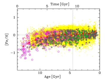
Figure 1: Observed Iron abundances [Fe/H] as a function of the stellar age, or the evolutionary time, upper-axis, for different authors as used in this work: small yellow dots from DR3-GALAH survey (Buder et al., 2018), green squares from Chen et al. (2000), orange triangles from GAIA (Bergemann et al., 2014), grey stars from HARPS-GTP (Bertran de Lis et al., 2015; Suárez-Andrés et al., 2016, 2017; Delgado Mena et al., 2017, 2019; Costa Silva et al., 2020), magenta open dots from AMBRE (Santos-Peral et al., 2020); (see summary Table 1). The binned values (computed in Appendix A) are overplotted on the series of data as red dots with error bars.

Table 1: Set of catalogues and references of used data.

Reference	Survey/Name	[Fe/H]	[O/Fe]	[Mg/Fe]	[Si/Fe]	[S/Fe]	[Ca/Fe]	[$\alpha$/Fe]	Age	[C/H]	[N/H]	Symbol
(1)	CHEN00	X	X	X	X	—	X	X	X	—	—	green square
(2)	GAIA-BER14	X	—	X	—	—	—	—	X	—	—	orange triangle
(3)	HYPATIA	X	X	X	X	X	X	X	—	X	X	cyan asterisk
(4,5,6,7,9,10)	HARPS-GTO	X	X	X	X	X	X	X	X	—	—	grey star
(8)	GALAH	X	X	X	X	—	—	X	X	X	—	yellow small dot
(11)	AMBRE	X	—	X	—	—	—	—	X	—	—	magenta open dot

(1):Chen et al. (2000); (2) Bergemann et al. (2014); (3): (Hinkel et al.2014); (4):Bertran de Lis et al. (2015); (5) Suárez-Andrés et al. (2016); (6): Suárez-Andrés et al. (2017); (7): Delgado Mena et al. (2017); (8): Buder et al. (2018); (9): Delgado Mena et al. (2019); (10): Costa Silva et al. (2020); (11):Santos-Peral et al. (2020)

2 Observational data: stellar catalogues

Stellar data will be used to compare with the [X/Fe] relative abundance from models and to be able to determine which of them is the best one to fit these data, the most ones affected by variations in DTDs and SN Ia yields. Here, we describe these data sets.

To compare the model predictions for the time evolution of the disc, we searched for observations of stars with available elemental abundances for Fe and for $\alpha$ elements (as many of them as possible) and also age estimates. We used here the stellar data from several authors/surveys, as given in Table 1, in particular those from Chen et al. (2000), the Hypatia catalogue (, Hinkel et al.2014), and the HARPS and GALAH samples, which fulfil these conditions.

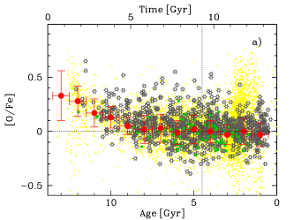
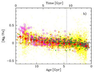
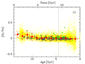
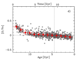
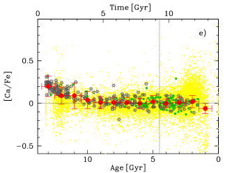
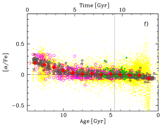
Figure 2: Observed $alpha$-elements over Iron abundances, [$X$/Fe], as a function of the stellar age, or evolutionary time in upper-axis, both in Gyr. Data correspond to different sets as summarized in Table 1 for each element $X$: Small yellow dots from DR2-GALAH survey (Buder et al., 2018), green squares from Chen et al. (2000), grey stars from HARPS-GTP (Bertran de Lis et al., 2015; Suárez-Andrés et al., 2016, 2017; Delgado Mena et al., 2017, 2019; Costa Silva et al., 2020), orange triangles from GAIA (Bergemann et al., 2014), magenta open dots from AMBRE (Santos-Peral et al., 2020). The binned values (computed in Appendix A) are overplotted over each series of data as red dots with error bars.

Chen et al. (2000) gathered high-resolution and high signal-to-noise (S/N) spectra for a sample of 90 F and G main-sequence disc stars. The observations were performed with the Coudé Echelle Spectrograph attached to the 2.16 m telescope at Beijing Astronomical Observatory (Xinglong, PR China). They provide metallicities in the range $-1.0<$ [Fe/H] $<+0.1$, with approximately the same number of stars in each metallicity bin of 0.1 dex. Stellar ages are also provided from interpolated evolutionary tracks. Their $\alpha$-chemical abundances for O, Mg, Si, Ca were used to compute the $[\alpha/\mbox{H}]$ ratio by assuming that $\alpha$-abundances are represented by the average of the aforementioned abundances.

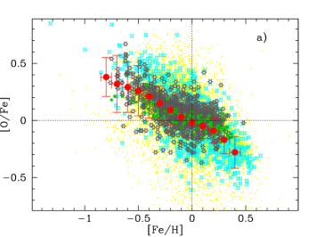
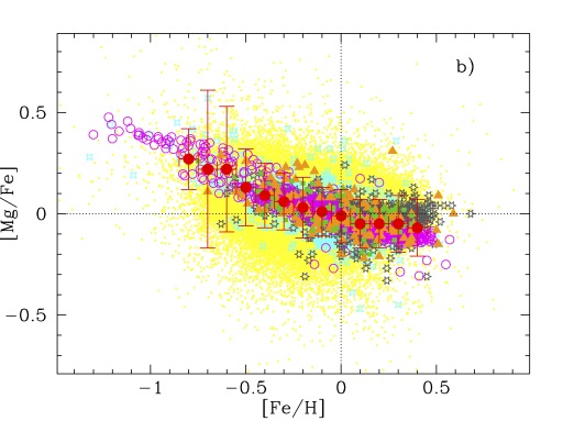
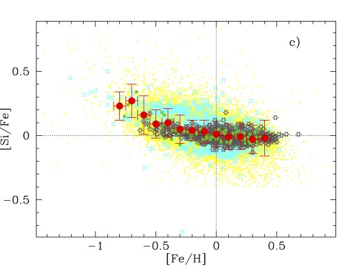
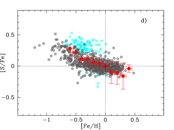
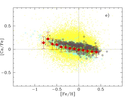
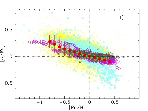
Figure 3: Observed alpha-elements abundances, [X/Fe], as a function of [Fe/H]. Data correspond to different sets as summarized in Table 1 for each element $X$: Small yellow dots from DR2-GALAH survey (Buder et al., 2018), green squares from Chen et al. (2000), grey stars from HARPS-GTP (Bertran de Lis et al., 2015; Suárez-Andrés et al., 2016, 2017; Delgado Mena et al., 2017, 2019; Costa Silva et al., 2020), orange triangles from GAIA (Bergemann et al., 2014), magenta open dots from AMBRE (Santos-Peral et al., 2020), and cyan asterisks from HYPATIA catalogue (, Hinkel et al.2014). The binned values (computed in Appendix A;) are overplotted over each series of data as red dots with error bars.

The stellar data from the Hypatia catalogue, as compiled by (Hinkel et al.2014) have been also taken. These authors compiled spectroscopic data from 84 literature sources with almost 10000 stars withing 500 pc around the Sun, for which they estimated abundances of different elements. Actually, for our plots we have taken the reduced version from the CDS-Strasbourg, with a total of 3058 stars in the solar neighbourhood, within 150 pc of the Sun, sufficient for our purposes. Since the catalogue is a compilation of a wide variety of sources that use different telescopes and instrumental configurations, as well as methods to derive abundances, we expect a larger spread in the chemical abundances than for others smaller and more homogeneous samples.

The HARPS (HARPS-GTO) sample is composed by the stellar data given in Delgado Mena et al. (2010, 2015); Bertran de Lis et al. (2015); Suárez-Andrés et al. (2016, 2017); Delgado Mena et al. (2017, 2019) and Costa Silva et al. (2020), which are compilations from the HARPS planet search programme, HARPS-1, observed with the UVES spectrograph installed at the VLT/UT2 Kueyen telescope (Paranal Observatory, ESO, Chile) during several campaigns. We have used the catalogues taken from the CDS-Strasbourg. Bertran de Lis et al. (2015) provide stellar parameters and abundances for 762 stars observed at high-resolution and high S/N. We prefer to use their oxygen abundances derived from both Oi 6300 Å  and Oi 6158 Å  lines, since they agreed within 0.1 dex in 58% cases. By using both lines, we incorporate the uncertainties in the oxygen abundance determinations in the data plots. We selected [N/H] and [Fe/H] abundances and stellar ages for 65 disc dwarf stars from Suárez-Andrés et al. (2016). In Suárez-Andrés et al. (2017) the [C/H], [Fe/H] abundances and stellar ages for 1058 FGK solar-type disc stars were selected. Delgado Mena et al. (2017, 2019) give abundances for Mg, Si, Ca and Costa Silva et al. (2020) for S. The HARPS data from these different authors are, in principle, compatible, since the abundances are calculated with the same methods and codes. Using all sets together, we will simulate the real dispersion of data due to different methods and instruments. Finally, in Delgado Mena et al. (2019) the stellar ages are obtained, allowing the analysis of the time evolution in the Solar vicinity.

We have also used the second data release of the European Space Agency Gaia astrometric survey, as obtained by the high-resolution Galactic Archaeology with HERMES (GALAH) spectroscopic survey (Buder et al., 2018). This survey aims at to analyse the structure of our Galaxy’s disc components using a large number of stars in the MWG by studying the kinematics and chemical abundances. The total number of stars from this DR2 is $\sim$ 340 000. However, not all of them have similar precision for stellar ages and abundances. We have selected stars with error in ages smaller than a 30%. We have also selected stars with height over the galactic plane $|z|<0.2$ kpc, and within the Solar distance, galactocentric distances in the range $7.5\leq R_{gal}\leq 9$ kpc, and we have restricted to good parallaxes with $eplx/plx<0.1$. Even with these cuts, the ages have large errors which, for the oldest stars, reaches to be as high as 3 Gyr, although the average value is slightly higher than 1 Gyr. This subsample, which consists of $\sim$ 105 000 stars, is used in our Fig. 1, and Fig. 2 and 3.

All these data are given using different Solar abundances, as shown in the Appendix A;, Supporting Information, Table 6. Therefore, in order to compare all of them, we have renormalized the data to the same Solar abundances scale from Lodders (2019). After this, differences in their scale could still be seen, since we consider that all abundances [Fe/H] and [X/Fe] must be zero for ${\rm[Fe/H]=0}$ and $\tau=4.6$ Gyr when $t=8.5$ Gyr, the time of the Sun’s birth. That is, the data must be around the Solar values at the Solar metallicity and age. We have therefore shifted each cloud of data to locate the Solar value in its centre.

Once in the same scale, abundances were binned, with values for each Gyr in the time evolution of [Fe/H] and [X/Fe] abundances, and for each dex as a function of [Fe/H]. The resulting data are represented in Figs. 1, 2 and 3 for the age-metallicity relation, and for the [X/Fe] relative abundances as a function of age and of [Fe/H], respectively. These bins are overplotted over the sets of data used with different symbols as given in Table 1, and are given in Tables  7, 8 and 9 of Appendix A where details about this process of normalization and binning of data are given.

3 Summary description of galaxy evolutionary models

Our MulChem chemical evolution models, particularly the one applied to the MWG, have been described in Mollá et al. (2015, 2016, 2017, 2019, hereinafter MOL15, MOL16, MOL17 and MOL19, respectively), updating the models from Ferrini et al. (1994); Mollá & Díaz (2005) for what refers to the inputs for modelling a given galaxy. We summarise the changes done in this new version of the Galaxy model, related with stellar yields and SN Ia DTD’s. The other model hypotheses and equations are described in the cited references.

3.1 Stellar yields.

To compute the elemental abundances, we use the technique based on the $Q$-matrix formalism (Talbot & Arnett, 1973; Ferrini et al., 1992; Portinari et al., 1998). Each element $(i,j)$ of a matrix, $Q_{i,j}$ gives the proportion of a star which was initially element $j$, ejected as $i$ when the star dies. Thus,

$$Q_{i,j}(m) = \frac{m_{i,j,exp}}{m_{j}},$$ (1)

$$Q_{i,j}(m)X_{j} = \frac{m_{i,j,exp}}{m},$$ (2)

where $m_{i,j,exp}$ is the ejected mass of an element $i$ initially being other $j$. These numbers must be multiplied by the number of stars of mass $m$, given by the used IMF, here being the one from Kroupa (2001, hereinafter KRO) with limits $m_{\rm low}=0.15$ M_☉ and $m_{\rm up}=40$ M_☉

In this work, the ejected mass from stars we use are the stellar yield sets from Cristallo et al. (2011, 2015), the FRUITY set, for low and intermediate mass stars, and from Limongi & Chieffi (2018) for massive stars. The first ones produced a first set of stellar yields for stars between 1 and 3 M_☉ in their work Cristallo et al. (2011), which is complemented with other set for masses in the range from 4 to 6 M_☉ (Cristallo et al., 2015). They follow carefully the evolution of each star, particularly the AGB phases with successive thermal pulses and dredge-ups. They give in their FRUITY web page (http://fruity.oa-teramo.inaf.it/) the complete information, stellar masses and core and surface abundances in each step, as well as the net and total yields for 400 isotopes and 10 metallicities. We have used their so-called total yields, which actually are the total ejected mass (new and already existing in the star when formed) of each isotope to include in our code, and this way to obtain the Q’s matrices for the eight stellar masses given by the authors. Moreover, using the information of the successive steps of the AGB stars evolution, that is, each remaining mass and the corresponding surface abundance, we have computed the secondary and primary components for ¹⁴N and ¹³C, by assuming that the production during the third dredge-up may be considered as primary and the rest is secondary. For massive stars, Limongi & Chieffi (2018) give the stellar yields for four metallicities ([Fe/H]=0, -1, -2, -3) and for nine stellar masses, from 13 to 120  M_☉ (http://orfeo.iaps.inaf.it). They calculated the same sets for three different values of the stellar rotation velocity: 0, 150 and 300 km s^-1, finding, in agreement with previous works (Meynet et al., 2006; Chiappini et al., 2011), that the rotation modifies the stellar yields, mainly the one for ¹⁴N, which appears as primary for low metallicities. In fact, since not all stars rotate at the same velocity, it is necessary to use a distribution of them for each metallicity. Following the recommendations of these authors, we have used the distribution shown in Fig.4 from Prantzos et al. (2018). Therefore, we have finally a mix of stellar yields at each rotation velocity for each one of the 4 metallicities. Then, we have interpolated at the same 10 metallicities as FRUITY for low and intermediate mass stars, to obtain a set of ejected masses for the whole mass range from 1 to 120  M_☉ and 10 metallicities. The stellar yield given by the authors for ²⁴Mg, ²⁸Si and ⁴⁰Ca have been multiplied by a factor of 2, 0.7 and 1.6, respectively, to better reproduce the observations. Finally, we added the stellar yields for SNe-Ia, see Section 3.3. These new yields were already included in Cavichia, Mollá, & Bazán (2023), successfully reproducing the Galactic bulge abundances ratios and their dependence along the evolutionary time. In this work we use starmatrix(Bazán & Mollá, 2022), an Open Source Python code that compute the new ejected elements by each SSP, then included in the MulChem model by a convolution with the SFR.

3.2 Supernova rates and delay time distributions for SNe Ia

We consider that all stars with $m>8$ M_☉ and $m\leq 40$ M_☉ will end their life as CC SNe (including all types together), although the limit of mass of stars that explode as CC SNe is under debate (Doherty et al., 2017). For a SSP, the total number of such events per unit stellar mass formed is thus determined by the IMF $\phi(m)$ as:

$$\frac{N_{CC}}{M_{*}}\simeq\int_{8\,M_{\sun}}^{m_{up}}\,\phi(m)\,dm,$$ (3)

which gives a value of $\sim 0.0052$ M_☉^-1 for a KRO IMF between 0.15 and 40 M_☉ ($\sim 0.054$ M_☉^-1 if m${}_{up}=100$ M_☉), and 0.0083 M_☉^-1 for a Salpeter (1955) IMF, within the same mass range. The IMF from Chabrier (2003) produces two times the number of the CC SNe created compared with a KRO IMF.

For an arbitrary star formation history, $\Psi(t)$, the instantaneous rate of CC SNe is given by:

$$\frac{dN_{CC}}{dt}(t)=\int_{8\,M_{\sun}}^{m_{up}}\Psi(t-\tau(m))\ \phi^{\prime}(m)\ dm,$$ (4)

where $\phi^{\prime}(m)$ denotes the adopted IMF subtracting the fraction of stars in binary systems that would yield SN Ia.

Table 2: DTD functions used in the models computed in this work.

Num.	Name	scenario	Delay	Reference	colour
1	CASTRIL	DD	50 Myr	Castrillo et al. (2021)	sea green
2	MAOZ017	DD	50 Myr	Maoz & Graur (2017)	light green
3	CHE2021	DD	140 Myr	Chen, Hu, & Wang (2021)	green
4	GRCDD04	Close DD	400 Myr	Greggio (2005)	dark green
5	GRWDD04	Wide DD	400 Myr	Greggio (2005)	orange
6	STROLG5	DD	$\upxi=-650$, $\Omega=2200$, $\alpha=1100$	Strolger et al. (2020)	coral red
7	GRCDD10	Close DD	1 Gyr	Greggio (2005)	red
8	GRWDD10	Wide DD	1 Gyr	Greggio (2005)	dark red
9	GRSDSCH	SD Mass sub-MCh	40 Myr	Greggio (2005)	maroon
10	GRESDCH	SD Mass Ch	100 Myr	Greggio (2005)	violet
11	STROLG1	SD	$\upxi=10$ Myr, $\Omega=600$, $\alpha=220$	Strolger et al. (2020)	lavander
12	STROLG2	SD	$\upxi=110$ Myr, $\Omega=1000$, $\alpha=2$	Strolger et al. (2020)	blue
13	STROLG3	SD	$\upxi=350$ Myr, $\Omega=1200$, $\alpha=20$	Strolger et al. (2020)	cyan
14	STROLG4	SD	$\upxi=6000$ Myr, $\Omega=6000$, $\alpha=-2$	Strolger et al. (2020)	light blue
15	RLPPC00	combined	several Gaussians	Ruiz-Lapuente et al. (2000)	magenta

In turn, the rate of SNe Ia explosions is given by the equation:

$$\frac{dN_{Ia}}{dt}(t)=\int_{\tau_{\rm min}}^{{\rm min}(t,\tau_{\rm max})}\frac{dN_{*}}{dt}(t-\tau)\ A_{Ia}\ DTD(\tau)\ d\tau,$$ (5)

which involves the total number of stars

$$\frac{dN_{*}}{dt}(t-\tau)=\Psi(t-\tau)\int_{m_{\rm low}}^{\rm m_{up}}\phi(m)\ dm$$ (6)

created per unit time at time $t-\tau$, the fraction of them ($A_{Ia}$) that eventually produce a SN Ia, and the delay time distribution $DTD(\tau)$ in terms of the age $\tau$.

If the IMF is normalised in mass, $\int_{m_{\rm low}}^{m_{\rm up}}m\ \phi(m)\ dm=1$, as usual, then $N_{*}=\int_{m_{\rm low}}^{m_{\rm up}}\phi(m)\ dm$ is the number of stars per unit stellar mass of a generation or single stellar population. This value depends again on the IMF, being 1.71 M_☉^-1 for the KRO IMF used here (2.02 M_☉^-1 for Salpeter). In that case, $N_{Ia}=N_{*}\times A_{Ia}$ gives the number of SN Ia produced by each stellar generation. Using observational data of SN Ia rates in galaxies, Greggio (2005) found a value $A_{Ia}\sim 10^{-3}\,\rm M_{\sun}^{-1}$.

This way, Eq. 5 may be written as:

$$\frac{dN_{Ia}}{dt}=N_{*}\times A_{Ia}\int_{\tau_{\rm min}}^{{\rm min}(t,\tau_{\rm max})}\Psi(t-\tau)\,DTD(\tau)\ dt.$$ (7)

The function $DTD(\tau)$ is the Delay Time Distribution that describes how many type Ia SNe progenitors die after a delay time $\tau$ for a simple stellar population (SSP) of mass 1 M_☉. This function is usually normalised, for the whole age of a galaxy, that is integrated along an age of 13.2 Gyr, to 1 :

$$\int_{\tau_{i}}^{\tau_{x}}DTD(\tau)\ d\tau=1,$$ (8)

where $\tau_{i}$ is the minimum delay, or minimum lifetime for one star precursor of a SN Ia. Since it is usually assumed that the SNe Ia occur in binary systems where the mass limits are assumed to be between 3 and 16 M_☉, $\tau_{i}$ would correspond to the age of the most massive component possible, that is 8 M_☉. For the upper limit, we need to choose between the longer age corresponding to the lower mass that could exist in a binary system, $\sim$ 1.5 M_☉ and, if the conditions allow it, the time in which the explosion may occur. In practice, this $\tau_{x}$ may be as long as the Hubble time.

Different progenitor scenarios for SNe Ia, and therefore different possible DTDs are at present supported by data. The MulChem model in its original form (Ferrini et al., 1992, 1994) used the technique explained in Greggio & Renzini (1983) to compute the SNe Ia rate from a secondary mass distribution. In more recent versions, from Mollá & Díaz (2005) until MOL19, the code incorporated the rates given by Ruiz-Lapuente, Canal, & Burkert (1997); Ruiz-Lapuente et al. (2000), who provided a numerical table (private communication) with the time evolution of the SN rates for a SSP, computed under different assumptions or scenarios and their probabilities of occurrence. The final function, called RLPC00, composed by several Gaussian functions, each one describing a given channel and showing a maximum at a different delay time, is shown in Fig. 4a). In this work, besides that RLPPC00 DTD, still used since it is useful to check the results of models, we have used other 14 DTDs more, as given in Table 2, obtained for both DD and SD scenarios by different authors, following theoretical (Greggio, 2005) or observational prescriptions.

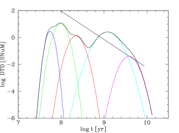
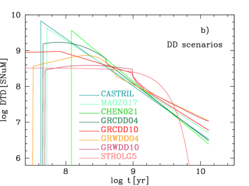
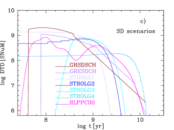
Figure 4: Theoretical and empirical DTD functions: a) the set of Gaussian curves, representing each one a different channels of SN Ia from RLPPC00, is shown as an example of combination of different channels. The straight line would correspond to an exponential function of slope $\beta=-1$; b) for DD scenarios; c) for SD scenarios, as given by authors showed in Table 2. RLPPC00 is also included in this panel although it represents a mix of scenarios; We have normalised all functions to give a value of 0.001 SN M${}_{\sun}^{-1}$ integrated along the life of the Universe. Each DTD is shown with a different colour as labelled. All SN rates are given in the usual unit of SNuM, number of SN that appear by 10¹⁰ M_☉ in 100 yr.

As explained in Section 1, there also exist some empirical works, which deduce the rate or DTD necessary to obtain a SN frequency as observed. In Maoz et al. (2011) a review about this technique is given. From an observational point of view, the first DTD studies from Mannucci et al. (2005, 2006) established a relationship between the SNR and the colour and Hubble type of the SN galaxy host, both measurements considered as approximations to the SFR. After these first attempts, Sullivan et al. (2006); Li et al. (2011a, b); Smith et al. (2012) found two populations of SNe Ia: one associated to the SFR with short delays of 100–500 Myr, the prompt population; and a tardy population associated to the galaxy mass and delays of up to 5 Gyr. However, more recent studies have found a general relation between the SNR and the age of the underlying stellar population, implying a continuous DTD proportional to $t^{-1}$ (Maoz &Mannucci, 2012b), a result supported by theoretical models for DD scenarios.

Measuring the SNR in galaxy clusters, a DTD also proportional to $t^{-1}$, but with delays longer than 2 Gyr up to 10 Gyr, was found (Barbary et al., 2012; Maoz et al., 2010). The same result was obtained for field elliptical galaxies (Totani et al., 2008). Thomson & Chary (2011); Raskin et al. (2009); Aubourg et al. (2008) also establish the existence of a prompt population that can dominate the SNR, even if the current SFR is small compared to the galaxy mass (Maoz &Mannucci, 2012b; Mannucci, 2009). More recently some works computed the DTD from the volumetric rate evolution of SN Ia. Large SN surveys are then necessary to infer the SNR, and the SFR comes from cosmological simulations (Graur & Maoz, 2013; Rodney et al., 2014; Friedmann & Maoz, 2018), from the modelling of the colours for the galaxy (Heringer et al., 2017, 2019), from the use of stellar population synthesis codes for individual galaxies (Maoz et al., 2012a), or even from integral field spectroscopy analysis of the host galaxies (Castrillo et al., 2021).

This way, some exponential functions variable with time from Maoz & Graur (2017), Castrillo et al. (2021), and Chen, Hu, & Wang (2021), valid for the DD scenario, are here used:

$$DTD_{\mathrm{MAOZ017}} = A\times e^{(-t/1.1)},\mbox{ if }t>\tau=50\,\mbox{Myr}$$ (9)

$$DTD_{\mathrm{CASTRIL}} = B\times e^{(-t/1.2)},\mbox{ if }t>\tau=40\,\mbox{Myr}$$ (10)

$$DTD_{\mathrm{CHE2021}} = C\times e^{(-t/1.41)},\mbox{ if }t>\tau=120\,\mbox{Myr},$$ (11)

where A, B and C are normalisation constants. We have also added other function, (STROLG5), as given by Strolger et al. (2020, their figure 5, right panel), obtained with parameters given in that figure. All these functions are represented in Fig. 4b), with different colour lines, as labelled. In most of the empirical works, the slope of the exponential function is in the range $\sim-1.1$ to -1.35: -1.1 for MAOZ017, -1.30 for Friedmann & Maoz (2018), -1.34 for Heringer et al. (2019), -1.1 for CASTRIL; while the delay time, $\Delta\tau$, as given in Eq. 11, is more variable: 40 Myr for CASTRIL, 50 Myr for MAOZ017, and 120 Myr for CHE2021. These last authors established that although their results indicates a high confidence of $\Delta\tau=120$ Myr, and their slope is -1, consistent with the DD scenario, they can not firmly eliminate other channels of SNe Ia with other times of appearance.

Some theoretical functions from Greggio (2005) are also used and included in that figure Fig. 4b). They are called GRCDD04 GRCDD10, GRWDD04 and GRWDD10, which correspond to the close and wide DD scenarios with time parameters 0.4 and 1.0 Gyr. They might be well represented by exponential functions as the observational ones for times later than some hundred of Myr (this is not the case for the STROLG5 DTD), but not for early times.

Moreover, we have also tried other DTDs that would correspond to the SD scenario. In that case, we have used the curves given by Greggio (2005) for her models SD with MCh and with sub-MCh (we call them as GRESDCH and GRSDSCH). To these theoretical prescriptions, we have added other 4 functions as given by Strolger et al. (2020, their figure 5, left panel), obtained by modifying the parameters of their equation to fit the observational data from Nelemans et al. (2001). All these functions and the one from RLPPC00, which is a mix of channels, are drawn Fig. 4c) with different colour lines as labelled.

Table 3: Set of yields for SNe Ia used in the models computed in this work.

Num.	Name	type of explosion	model/table	reference	type of line
1	IWA1999	MCh	fast deflagration W7/W70	Iwamoto et al. (1999)	solid
2	SEI2013	MCh	DDT Table 2-N100	Seitenzahl et al. (2013a)	light solid
3	MO20181	MCh	W7 DDT model Table 3	Mori et al. (2018)	dotted
4	MO20182	MCh	WDD2 DDT model Table 3	Mori et al. (2018)	light dotted
5	LN20181	Near MCh	DDT Table 3, low $\rho$	Leung & Nomoto (2018)	short-dashed
6	LN20182	Near MCh	DDT Table 4, medium $\rho$	Leung & Nomoto (2018)	light short-dashed
7	LN20183	Near MCh	DDT Table 5, high $\rho$	Leung & Nomoto (2018)	long-dashed
8	BR20191	MCh	DDT Table 3	Bravo, Badenes, & Martínez-Rodríguez (2019)	dot-short-dashed
9	BR20192	sub-MCh	Table 4	Bravo, Badenes, & Martínez-Rodríguez (2019)	light dot-short-dashed
10	LEU2020	sub-MCh	DDet Table 7	Leung & Nomoto (2020)	short-long-dashed
11	GR20211	sub-MCh	DDet with He shell, Table A10, Table 3	Gronow et al. (2021)	dot-long dashed
12	GR20212	sub-MCh	DDet with He shell, Table A8, Table 4	Gronow et al. (2021)	light dot-long dashed

Some years ago, Mennekens et al. (2010) did synthesis of populations to produce models of SD and DD scenarios. They compare the resulting DTD curves with observational data (Mannucci et al., 2005; Totani et al., 2008), as seen in their figure 2. They show that the SD scenario produces a maximum in 1.4 Gyr and then they disappear after 8 Gyr. The DD scenario creates a curve proportional to $t^{-1}$ and it is the dominant channel. However, the SD alone does not fit the observed distributions, being DD or a mix of both channels SD$+$DD the most probable scenario. In fact, in that figure they presented a mix of both channels that reproduce well the data. Similarly, Ruiter et al. (2009); Ruiter et al. (2011) did similar models for 4 scenarios: DD, SD and HeR with MCh, and one double detonation sub-MCh scenario involving helium-rich donors. He computed the DTDs for the 4 cases, and comparing with the observations he shows that the Sub-MCh may create both, a prompt ($<500$ Myr) channel, and a more delayed ($>500$  Myr) one.

Such as Nelemans, Toonen, & Bours (2013) claimed, "the observed SN populations probably originated from a combination of multiple channels". That is, although the SNe Ia scenario defines mainly the delay time for the explosion will occur, a diversity of models is possible due to the different mass accretion rates, the existence or not of winds, the stripping rate of the companion, or the variations to radiate away the angular momentum, which change the time necessary to have a explosion in the DD scenario. Thus, theoretical models give delay times between 0.5 to 3 Gyr for SD scenarios and a mean time larger than 0.3 Gyr for DD scenarios. In fact, there is not an unique model able to reproduce satisfactory the diversity of observations of SNe Ia. It is, therefore, quite probable that several channels be mixed to produce the SNe Ia observed distribution (Mernier et al., 2016; Hitomi Collaboration et al., 2017). Although we have mainly used only one DTD in each model, except when using RLPPC00 that is by itself a mix of scenarios, it is necessary to take into account that the most probable solution will need two or more DTDs, either simultaneously or varying along the time, in the same model.

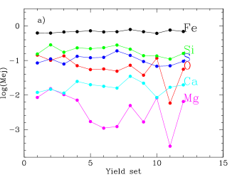
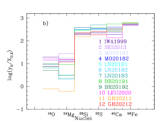
Figure 5: Yields of different elements as ejected in the 12 different explosions models included in this work, numbered as given in Table 3: a) yields given as the ejected mass (logarithmic scale), $\log{M_{\mathrm{e}j}}$, from ¹⁶O to ⁴⁰Ca plus ⁵⁶Fe; b) zoom of the $\alpha$-elements yields from ¹⁶O to ⁴⁰Ca and the one of ⁵⁶Fe, given as the ratio of the ejected mass by Solar abundances, $\log{y_{i}/X_{\sun}}$ from different authors as labelled.

3.3 The SN Ia element yields

As explained above, there are a variety of possible thermonuclear explosions models, which produce elements in different quantities (Arcones & Thielemann, 2023). The explosion mechanisms may be due to different situations, which are widely explained in Liu, Röpke, & Han (2023, see their table 1 and Fig.3) and summarized as: 1) The burning of C in the centre of the star, when the WD reaches the MCh (the classical case): the simmering phase starts, with the consequent compression heating and a central burning that produces the thermonuclear runaway. 2) The burning of C in the outer envelope, outer ignition. That occurs with a merger of two WD (Double degenerate WD scenario). 3) The burning of He, which starts in the surface of the star, when He is accreted from a companion rich in helium (He-WD or CO-WD with He envelope). This burning provokes a shock wave toward the centre of the WD and produces a WD detonation.

There exist differences in the described mechanisms, since the flame propagation may occur with different velocities: a) detonation, when the burning occurs at supersonic velocities; b) deflagration, when the burning occurs at subsonic velocity; and c) when a deflagration to detonation transition (DDT) occurs.

For this particular subsection we are interested in works where the nucleosynthesis yield sets are calculated for the different models. We refer to Table 3 for the details about the computed models in this work (Iwamoto et al., 1999; Seitenzahl et al., 2013a; Mori et al., 2018; Leung & Nomoto, 2018; Bravo, Badenes, & Martínez-Rodríguez, 2019; Leung & Nomoto, 2020; Gronow et al., 2021). These models are divided in two categories:a) those where the explosion occurs at MCh, and b) those where it occurs at sub-MCh. The first ones are usually computed for a delayed detonation (DDT) channel in a SD or DD scenario; while the second ones are calculated for the double detonation (DDet) case in a SD scenario, or for the merging of two WD (violent mergers) in a DD scenario. Therefore, although a priori there is not a direct correlation between the SN Ia scenarios and the explosion mechanisms, there are some limitations: the SD scenario can not produce an outer ignition, while triple systems occurs basically with outer C ignition. The intermediate case core degenerate (CD) scenario, does not occur with surface He-burning. But both scenarios SD and DD may occur with any mode of explosion. The key ingredient to obtain a SNe Ia is the density and temperature in the burning time. This determines the ejected quantity of ⁵⁶Ni.

After the seminal work from Nomoto (1982) with the classical W7 model, the revised model by Iwamoto et al. (1999) is the most frequently adopted in chemical evolution studies. The W7 model adopts a pure deflagration schema in a DD scenario, and was conceived to reproduce the observational data, so that there are inherent physical limitations and additional 1D modelling limitations. The yields were calculated for solar metallicity and a 1/10 of the solar value. This group also studied a slow delayed detonation with DDT and a channel CD.

Later, Seitenzahl et al. (2013a) presented results for a suite of 3-dimensional, high-resolution hydrodynamical simulations of delayed-detonation explosions (DDT) giving four datasets for ${\mathrm{[}Fe/H]}=-2$, -1, -0.3 and 0. In this model, the detonation is delayed with three phases: 1) There is a deflagration with burning in a high density core; 2) The energy propagates with subsonic velocity and the star expands, so the density is now lower. 3) A detonation occurs after a time. Seitenzahl et al. (2013b) found that the yields show a great dependence on metallicity in both CC SN and SNe Ia, finding that the 50% of SNe Ia would have explode as near-MCh WDs to reproduce the observations related to [Mn/Fe].

In last years, an increasing number of works, from which we have selected some of them to use in this work (Leung & Nomoto, 2018; Mori et al., 2018; Gronow et al., 2021), have computed models of explosions giving the yields of elements created by them, by using different thermodynamics conditions (central densities, velocities, turbulent velocity fluctuations, different strengths of the deflagration phase,…), which also allow the explosions for mass below the Chandrasekhar mass (sub-MCh). Also, there are two sets from Bravo, Badenes, & Martínez-Rodríguez (2019) giving yields able to reproduce the observations of SN Ia. In turn, Leung & Nomoto (2020) have revised the W7 model for a MCh deflagration explosion with improvements on the nuclear reaction network in comparison with those from Iwamoto et al. (1999), also included in our set of yields.

The yields of different elements ejected used in this work correspond to twelve different sets obtained for different explosion mechanisms and given in Table 3, where we define for each set a number (column 1) and an acronym or name of the yield set (column 2) that we will use later for identifying each one. The third column displays the type of explosion, the fourth column the chosen model or table, the fifth column the source reference, and the sixth column the line style to plot the models in the next figures. In some cases the authors give more than one table, and we have selected one or more sets following their recommendations. All of them are plotted in Fig. 5. In panel a) we represent the ejected mass of each element as a function of the number of the yield set (column 1 of Table 3); In panel b), we represent the abundance compared with the solar one from Lodders (2019) as a function of the mass number A of each nuclei. Each set is drawn with a different colour as labelled. The yield for Fe, the most important element in this case, is essentially the same for all of them. For O, except GR20211, Si, and S, all tables give results within an order of magnitude. There are, however, important variations in the yields for ²⁴Mg and ⁴⁰Ca among the different sets, where models GR20211, LN20182 and BR20192 show the lowest yields values.

4 Results

We have computed 180 models for MWG with fifteen different possibilities of DTD functions, representing different scenarios for the binary systems and their evolution, as shown in Table 2, combined with twelve different set of yields for different explosion mechanisms for the SNe Ia, as shown in Table 3. As it is said in the Introduction, not all combinations of DTD-SN yields are compatible with our knowledge about SN Ia scenarios and channels. Thus, yields computed for delayed detonation/DDT models with MCh explosions are compatible with DTD computed for SD scenarios, but the DDT explosion is also possible in the DD scenario; In turn, yields for sub-MCh are calculated for double detonation (DDet) channels in a SD scenario. The merging of two WDs as violent mergers may also may occur at sub-MCh. However, we have not used any set of yields valid for this case, and this way, yields sets for sub-MCh are here only valid for the DDet explosions in SD scenarios. The combinations sub-MCh yields $+$ DD DTDs that we have among the 180 computed models are not realistic in this work and these combinations must be interpreted with caution.

Our computations are based on the same model from MOL19, with the same total mass radial distribution, collapse time scales, and star formation efficiency for MWG. We have, however, updated the stellar yields to the those from Cristallo et al. (2011, 2015); Limongi & Chieffi (2018), and we have also modified the stellar mean-lifetimes. For that reason, we have checked in Appendix B, Supporting Information on the publication, that models give, for the quantities not related with Fe or $\alpha$-element abundances, the same results than in previous works, reproducing equally well the MWG data: SFR and the time evolution of CNO abundances for the Solar Region, and the radial distributions of SFR, mass of gas and stars, and CNO abundances in the Galactic disc, all of them compiled in MOl15.

Now, we investigate the model results in the Solar Region for what refers to the SN rates, the time evolution of Fe abundance and [X/Fe] data, particularly those of [$\alpha$/Fe], which depend on the proportion of CC SNe against SN Ia. In order to select the best combination of yields and DTDs, we have used a $\chi^{2}$ technique.

4.1 Supernova rates in the MWG

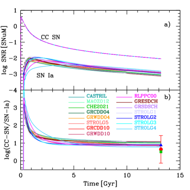
Figure 6: a) Time evolution of the SN rates, in SNuM units, for CC SN and SN Ia. The CC SN rates evolution fall in the same line for all models with a value of $\sim-2$ for the present time, about one dex above the SN Ia rate. The SN Ia rates vary, as shown different colours, depending on the used DTD. b) Ratio between both SN-II/SN Ia, compared to different theoretical estimates, blue and green dots from Maoz & Graur (2017); Greggio (2005), respectively, and observational estimates, red dot with error bar, averaged value from Mannucci et al. (2005); Maoz et al. (2014); Li et al. (2011a).

Once our models be well calibrated, we proceed to analyse the results related to the SN rates. Panel a) of Fig. 6 shows the evolution of both the CC SN and SN Ia rate as a function of time. Since the same IMF is used for all models, the CC SN rate is basically the same for all of them, as shown by the (overlapping) lines located in the upper side of the panel a). In contrast, the SN Ia rate evolves differently in each model, according to the used DTD. Thus, SN Ia appear at a different time for each DTD ( see delay times in Table 2), although it is difficult to see it at the scale of the age of the Universe. The first to appear is the STROLG1 (lavander line), with $\Delta t=10$ Myr, followed by GRSDSCH, CASTRIL, and MAOZ017, while the last ones are RLPPCC00, STROLG3 and STROLG4. In panel b), it is shown how the ratio between both types of SN changes among models. The lowest value at the present time corresponds to STROLG4 (0.78) and the highest one is for GRSDSCH (1.09). In the same panel, we also represent the ratio $N_{\rm CC}/N_{\rm Ia}$ from Maoz & Graur (2017), as a green square, and the ratio around $\sim 5\text{---}7$ (depending on the IMF) advocated by Greggio (2005) for a SSP as a blue triangle.

From an observational point of view, this ratio is dependent on the selected galaxy sample, varying with morphological type and $B-V$ colour (Li et al., 2011b). Being affected by the star formation history, we do find that it changes according to the radial region, although we only represent here the Solar region. Following Mannucci et al. (2005); Maoz et al. (2014); Li et al. (2011a), the observed ratio between CC and Ia SNe may be as small as 1 (or even lower than 1) or as large as $\sim 200$. This range is illustrated by a red dot with error bars. Thus, all used DTDs give equally acceptable results within the range defined by the error bars.

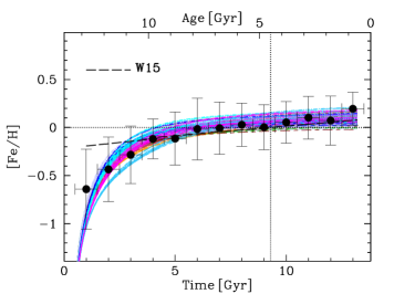
Figure 7: The time evolution of metallicity, as Iron abundance [Fe/H] for the Solar vicinity. Black dots are the binned data (see Section 2). The dotted lines indicate the Sun position at its birth’s time, 4.6 Gyr ago, for reference. Different models are plotted as lines following the style and colour scheme given in Tables 2 and 3 and Fig. 6. The straight dashed black line is the fit found by Walcher et al. (2015). Only the 148 realistic models are drawn.

4.2 The time evolution of metallicity and alpha-over-iron relative abundance on the solar vicinity

Now, we will compare the results related with the time evolution of the abundance for Iron [Fe/H] and $alpha$-elements [X/Fe] for the 148 models considered as realistic within our calculations. In Fig. 7, we display the age-metallicity relation for the Solar region, the metallicity being represented by [Fe/H]. Some combinations reproduce the data better than others, however, it is very difficult to choose the best model, given the high dispersion of data shown by the error bars of binned data represented by black dots.

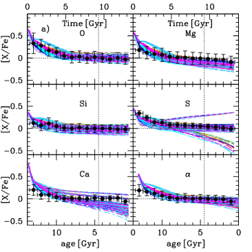
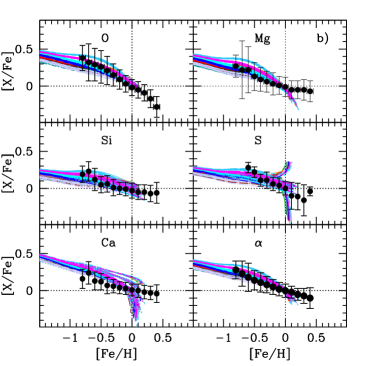
Figure 8: The relative abundances of [O/Fe], [Mg/Fe], [Si/Fe], [S/Fe], [Ca/Fe] and [$\alpha$/Fe] as a function of: a) the stellar age $\tau$ or time (in Gyr); b) the metallicity [Fe/H] for the 148 realistic models. Different models are represented by different colours and types of lines following the same style and colour scheme as in Fig. 7. Black dots with error bars represent the binned data as given in Section 2. The dotted lines indicate the Sun position for reference.

The next step is to analyse the evolution of different $\alpha$-elements relative abundances [X/Fe], which incorporate both CC and Ia SNe ejecta. In Fig. 8, left panel a), we present the relative abundances [X/Fe] for elements O, Mg, Si, S and Ca and the total [$\alpha$/Fe] ratio as a function of the stellar age $\tau$. We put the x-axis in reverse, that is the oldest ages on the left, and the youngest on the right. This way, it is easier to see the evolutionary sequence in terms of time, also shown in upper x-axis. In all plots, each set of a different colour shows models for a given DTD (with the same colour meaning as in previous figures). As before, the different yields from SN Ia have a smaller effect over the plots compared with the DTD and the results show a dispersion around each colour/DTD. From the Solar age (dotted vertical line) until now, all models follow a similar behaviour with differences only in the absolute abundances for O, Mg, Si and $\alpha$, while S and Ca show quite important differences in this last evolution times for some particular SN Ia yield sets. For S, LN20181 –short-dashed lines– gives results higher than observations, and LN20183 –long dashed lines– gives lower values than the data. For Ca, LEU2020 gives results well down of the data points from the Solar birth time until the present time for all DTDs.

The most important point here is that the relative abundances [X/Fe] are high compared to the Solar values for early times/old stellar ages. At these ages, elements produced by massive stars appear first. Later, Fe abundances start to increase in the ISM and the relative abundances decrease. From an evolutionary point of view the relative abundances [X/Fe] begin to decrease just when the first SN Ia explode, and, obviously the time when this occurs is very dependent on the DTD. Following these plots, models using CASTRIL and STROLG1 are the closest ones to the data for ages larger than 10 Gyr (early times). This is expected since these DTDs produce SN Ia very promptly once binary systems are created, as indicated by the delay times $\Delta t=40$ Myr in the first case, and by the parameter $\upxi=10$ Myr in the second one. The STROLG4 models –light blue lines– DTD show a bump for all elements at early times (old ages) that does not exist in the data trends doing this DTD invalid for our purposes.

In Figure 8, right panel b), we plot the same relative abundances [X/Fe] but now as a function of [Fe/H], following the same structure as before. To use [Fe/H] as a proxy of time has the advantage of eliminating the stellar age uncertainties, since only abundances are involved. It is thought, as other authors have claimed before, that the difference between SD-DTDs and DD-DTDs is that the first ones produce an early flat behaviour in [X/Fe] vs. [Fe/H] plots, maintaining a horizontal line until metallicities around -0.5 dex at least, and then an abrupt decrease for [Fe/H] $\sim 0$. On the other hand, the second ones would show a continuous decreasing line in the same plots. In Kobayashi, Leung, & Nomoto (2020, see their figure 18 top-left panel) is presented the plot for [O/Fe] vs. [Fe/H] considering a MCh case and a sub-MCh case (and some different proportions of both) associated to SD and DD scenarios, respectively. (In their results it is claimed that a combination with a $25\%$ sub-MCh SNe Ia and a $75\%$ MCh SNe Ia reasonably reproduces the observational constraints). We see, however, that different slopes, not only two behaviours, appear for our set of models with different DTDs. The flatter line is the one from STROLG4 –light blue lines–, while the steeper ones correspond to STROLG1, STROLG2 and STROLG3, –lavander, blue and cyan lines–, all of them corresponding to a SD mechanism. The plateau also appears for STROLG5, GRWDD04 and RLPPC00 with a DD scenario.

Not all models are broadly compatible with the observational data. In fact, it seems difficult to find -at naked eye– a model able to reproduce simultaneously the data in all panels (see next sections). Thus, the best models for S and Ca seem to be the ones in the lower part of plots, (STROLG1 models, lavander lines), while O, Mg, Si and $\alpha$ data are better fitted with STROLG5 –coral lines–, and other DTDs corresponding to DD scenarios as GRWDD04 –orange lines , or RLPPC00 models (magenta lines), but also by STROLG2,STROLG3 (blue and cyan lines), or GRESDCH –violet lines–, which corresponds to a SD scenario. For S, the two set of yields that show in panel a) lower and higher values as data in the present time, also show in panel b) a strange behaviour in disagreement with observations. The same occurs with Ca at the later times, where models decrease below the observations at present time.

Table 4: Values of $\chi^{2}$ for each set of observations $j$ ($j$=1,13) for the 180 computed models.

DTD	SNIa	$\chi^{2}_{1}$	$\chi^{2}_{2}$	$\chi^{2}_{3}$	$\chi^{2}_{4}$	$\chi^{2}_{5}$	$\chi^{2}_{6}$	$\chi^{2}_{7}$	$\chi^{2}_{8}$	$\chi^{2}_{9}$	$\chi^{2}_{10}$	$\chi^{2}_{11}$	$\chi^{2}_{12}$	$\chi^{2}_{13}$
	yields	[Fe/H]	[O/Fe]	[Mg/Fe]	[Si/Fe]	[S/Fe]	[Ca/Fe]	[$\alpha$/Fe]	[O/Fe]	[Mg/Fe]	[Si/Fe]	[S/Fe]	[Ca/Fe]	[$\alpha$/Fe]
		vs time	vs stellar age						vs [Fe/H]
(1)	(2)	(3)	(4)	(5)	(6)	(7)	(8)	(9)	(10)	(11)	(12)	(13)	(14)	(15)
CASTRIL	IWA1999	0.3791	0.1800	0.6151	0.4935	0.6588	1.7829	0.4940	0.2750	1.7261	0.3646	1.7967	0.7565	0.1704
CASTRIL	SEI2013	0.2269	0.1801	0.3803	0.5153	0.7103	1.5738	0.5095	2.4267	3.5518	2.8310	2.4128	4.1362	3.5639
CASTRIL	MO20181	0.3372	0.1629	0.5718	1.1162	2.0193	5.1793	0.7426	0.2910	1.8069	1.0382	1.3953	4.2580	0.9978
CASTRIL	BR20192	0.2269	0.4193	0.2383	0.3791	6.4963	10.7044	0.7612	4.8379	2.8879	1.3638	5.4288	7.8021	5.0884

We see in Fig. 8, that any models do not reach the metal-rich end ([Fe/H] > 0.2) observed in the stellar data. On the other hand, as we see in Fig. 7, [Fe/H] vs. time, that no model is richer than 0.2 dex. Since that curve shows the enrichment of the Solar region, probably the fact of having stars with metallicity higher than 0.2 dex in Fig. 8, which do not appear in Fig. 7, is related with measurements of other radial regions of the disc, which may be explained by the difficulties in estimating both, stellar ages and galactocentric distances, or by the possible migration of stars from their birth location.

4.3 Selecting the best models

In order to select the best models able to reproduce our sets of data simultaneously, we have performed a $\chi^{2}$ technique. We use the set of binned data described in Section 2 and compared with the corresponding results in each model. The observational binned data have 13 points for the time evolution of [Fe/H], 13 points of [X/Fe] abundances vs the stellar age, and other 13 points for the relative abundances [X/Fe] vs. [Fe/H].

We calculate for each model defined for $nmod$:

$$\chi^{2}_{j,nmod}=\sum_{i=1}^{np}\frac{(X_{{\rm mod},i,j,nmod}-X_{{\rm obs},i,j})^{2}}{\sigma^{2}_{i,j}},$$ (12)

for each quantity or data set, defined by $j$, where $X$ represents each abundance ([Fe/H] or [X/Fe]) for each observed and modelled point $i$, which also varies from 1 to 13 in the 13 sets of data. And $\sigma_{i,j}$ is the error of each observational point $i$ in each set of data $j$. We obtain 13 values of $\chi^{2}$ one for each quantity $j$ for each one of our models in the range $nmod\in[1,180]$.

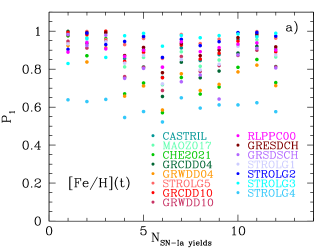
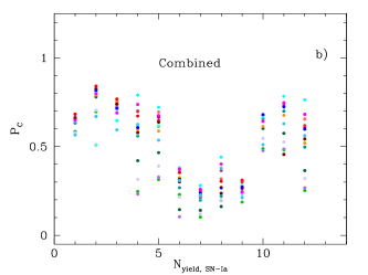
Figure 9: The resulting likelihood values: a) P₁; b) Combined P_C, as a function of SN-Ia yields (from 1 to 12) in x-axis. Colours indicate the different DTDs with same meaning as in previous figures. Only combinations considered realistic are plotted.

An example of the resulting $\chi^{2}_{j}$ is given in Table 4 and the complete table is available in electronic format. Columns (1) and (2) give the DTD and the SN-Ia yields, respectively. Column (3) gives the $\chi^{2}$ obtained for the age-metallicity relation, that is the [Fe/H] abundance as a function of time. Then, next six columns (4), (5), (6), (7), (8) and (9) correspond to the $\chi^{2}$ values obtained the comparison of the relative abundances [X/Fe] for O, Mg, Si, S, Ca, and global/average $\alpha$ as a function of the stellar age. Finally, columns (10), (11), (12), (13), (14) and (15) give the $\chi^{2}$ values obtained the comparison of the relative abundances [X/Fe] for O, Mg, Si, S, Ca, and global/average $\alpha$ as a function of [Fe/H].

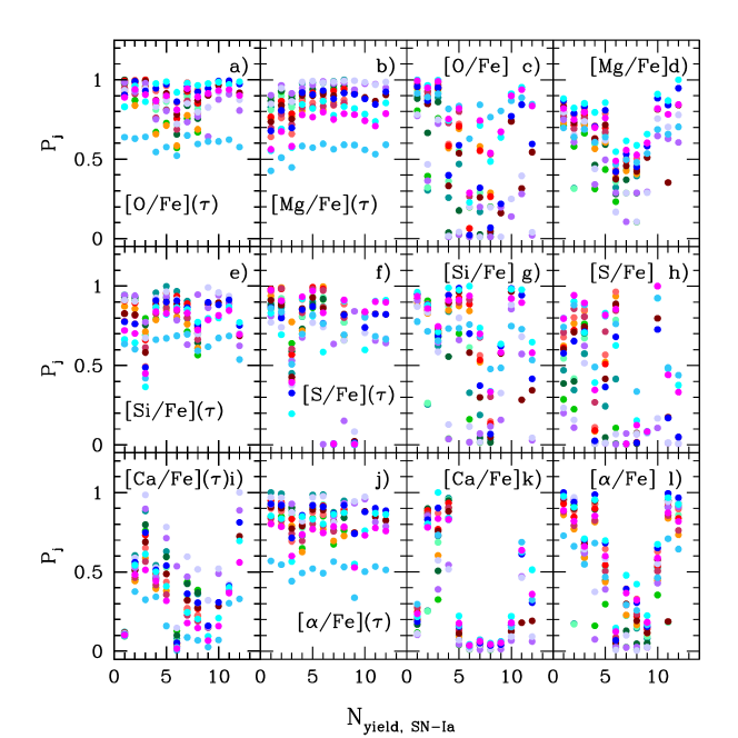
Figure 10: The resulting likelihood values, P_j for each set $j$ of data, from 2 to 13, compared with the models represented as a function of SN-Ia yields (from 1 to 12) in x-axis. Colours indicate the different DTDs with same meaning as in previous Fig.  9. Left six panels represent the probabilities around the best model obtained from the comparison model-data for [X/Fe] vs. age (represented by $\tau$). Right six panels represent the probabilities around the best model obtained from the comparison model-data for [X/Fe] vs. metallicity (represented by [Fe/H]). Only combinations considered realistic are plotted.

Although Table 4 gives the $\chi^{2}_{j}$ values for the whole set of models, that is for all possible combinations DTD$+$ yields set, we know that some models are not realistic in the context of this work with the set of DTDs and yields we are using. We have, therefore, suppressed for the analysis those models with DD scenario $+$ sub-MCh explosions, keeping the remaining 148 models.

After selecting the minimum value $\chi^{2}_{\rm min,j}$ for each observational data set $j$ we compute:

$$\chi^{2}_{{\rm red},j,nmod}=\chi^{2}_{j,nmod}-\chi^{2}_{\rm min,j}.$$ (13)

Once computed these values, we calculate the likelihood or confidence level, $P_{j}$ around the minimum value, (which would correspond to the maximum likelihood that we name $L_{max}$), given by:

$$P_{j,nmod}= 1-\alpha(\chi^{2}_{{\rm red},j,nmod}<x)=1-\int_{0}^{x}{\chi^{2}_{k}du}$$ (14)

$$= 1-\int_{0}^{x}{\frac{u^{k/2}e^{-u/2}}{2^{k/2}\Gamma(k/2)}du},$$

Table 5: The selected models: the best models obtained with $\chi^{2}_{\rm min}$ for each data set separately, after eliminating the non-realistic models.

Function	$L$	DTD	Scenario	Yields-SN-Ia	expl. type	$\chi^{2}_{min}$	$L_{max}$	Q
(1)	(2)	(3)	(4)	(5)	(6)	(7)	(8)	(9)
[Fe/H]($t$)	P1	STROLG5	DD	IWA1999	MCh	0.0519	0.9744	C
$\rm{[O/Fe]}(\tau)$	P2	GRCDD10	DD	MO20181	MCh W7	0.1562	0.9249	C
$\rm{[Mg/Fe]}(\tau$)	P3	CASTRIL	DD	BR20191	MCh	0.2361	0.8887	D
$\rm{[Si/Fe]}(\tau$)	P4	CASTRIL	DD	LN20181	MCh	04453	0.8004	D
$\rm{[S/Fe]}(\tau$)	P5	GRWDD04	DD	LN20182	MCh	0.4329	0.8054	C
$\rm{[Ca/Fe]}(\tau$)	P6	STROLG1	SD	GR20211	Msub-MCh	1.3721	0.50436	B
$[\alpha/\rm{Fe}](\tau$)	P7	CASTRIL	DD	IWA1999	MCh	0.4940	0.7811	D
$\rm[O/Fe]([Fe/H])$	P8	STROLG3	SD	IWA1999	MCh	0.0531	0.9738	A
$\rm[Mg/Fe]([Fe/H])$	P9	STROLG3	SD	GR20212	sub-MCh	1.2580	0.5331	B
$\rm[Si/Fe]([Fe/H])$	P10	STROLG3	SD	LN20182	MCh	0.0973	0.9525	A
$\rm[S/Fe]([Fe/H])$	P11	RLPPC00	MIX	LEU2020	sub-MCh	0.2869	0.8664	D
$\rm[Ca/Fe]([Fe/H])$	P12	STROLG3	SD	GR20211	sub-MCh	0.5662	0.7539	B
$[\alpha/\rm{Fe}](\rm{[Fe/H]})$	P13	STROL2	SD	IWA1999	MCh	0.0736	0.9639	A
Combined	PC	GRCDD10	DD	SEI2013	MCh		0.840	C

being $k_{j}=NF=2$, the number of degrees of freedom in this case, since we may change DTD or SN-Ia yields from a model to other one. In this expression, each model is assumed as represented by a $\chi^{2}$ distribution, $\alpha$ being the significance level associated with each $\chi^{2}$. By computing these likelihood values $P_{j}$, we may discriminate which are the best models around the value $L_{\rm max}$, whatever this value, which corresponds to the $\chi^{2}_{\rm min}$.

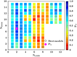
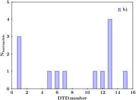
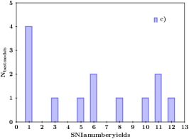
Figure 11: The summary of results for our models. Left panel represents the plane SN-Ia yields (with number from 1 to 12) – DTDs (with number from 1 to 15) in x and y-axis, respectively, with a colour scale given by the combined probability $P_{C}$, where we have suppressed the models DD$+$sub-MCh. Over the whole values of the plane, diamonds indicate the 13 models selected with each set of data individually, that is for each $P_{j}=1$. The magenta dot indicates the combination for which $P_{C}$ takes its maximum value. Middle and right panels represent histograms with the DTDs and yields of the 13 selected models.

We represent the resulting likelihood P_j obtained from the 148 values of $\chi^{2}$ in Fig. 9 and 10, as function of the number that define the set of SN-Ia yiels (see Table 3). Different colour points represent different DTDs as labelled. In Fig. 9a, the values corresponding to the age-metallicity relation, $P_{1}$, are shown, where all models have values $P_{j=1}>0.5$. In Fig. 9b, we show the combined $P_{C}$, computed as geometrical average of $P_{j}$:

$$P_{C}=\left(\prod_{i=1,13}^{13}{P_{i}}\right)^{1/13}$$ (15)

In Fig. 10, we show the values $P_{j}$ with j=2,7 in six left panels a), b), e), f), i) and j) , that correspond to the fit of each relative abundance [X/Fe], for O, Mg, Si, S, Ca and the global $\alpha$, as a function of the age, $\tau$. In right six panels, c), d), g), h), k) and l), we represent the equivalent $P_{j}$ with j=8,13 that correspond to the fit of each relative abundance [X/Fe], for O, Mg, Si, S, Ca and the global $\alpha$, as a function of [Fe/H]. All of them are represented as a function of the stellar yield number –given in Table3, with colour of points indicating each DTD. We see that there is no clear result giving a good solution for the whole set of observations. Thus, e.g. for [O/Fe] vs. age, the best models correspond to the lowest number of yields, while for [Mg/Fe]($\tau$) the maximum appears at intermediate values. When comparing with the corresponding right panels representing the goodness of the fits for correlations as a function of [Fe/H], the [Mg/Fe] need yields of low or high numbers, with a minimum just for the intermediate ones. The global result given by $P_{C}$ indicate better solutions for the classical SN-Ia yields 1 and 2 (IWA1999 and SEI2013) for MCh explosions or for the most recent 10 to 12 yields, (LEU2020, GR20211 or GR20212), computed for sub-MCh. Therefore, it is difficult to discriminate which explosion mechanism is the best one to reproduce the alpha-element over Iron abundances. It is also clear that some DTDs produce worse results than others, as it occurs with STROLG4 (light blue dots), with $P_{1}$ well below a 80%, and low values $P_{j}$ in general.

We give the best models fitting each set of data in Table 5, where for each data-model comparison in column 1, the name given to the likelihood for each one is in column 2, the DTD and the type of scenario are in columns 3 and 4, the SN-Ia yields set and the explosion type are in columns 5 and 6, the corresponding $\chi^{2}_{\rm min}$ is in column 7, and the corresponding maximum likelihood associated to that value is in column 8. We may see that not all sets are equally well fitted with their best model. Thus, [Fe/H](t) has value $L_{1}=0.974$, while [Ca/Fe]($\tau$) has a much lower $L_{6}=0.504$. The last row gives the maximum value for $P_{C}$ obtained as a combination of the 13 values $P_{j}$ (Eq.15) which gives a probability of $L_{max}=84$%.

These results are summarized in Fig. 11. In the left panel, we represent the plane SN-Ia yields number (x-axis) vs. the DTD number (y-axis), with a colour scale based in the value of the combined/averaged probability $P_{C}$. Over this plane, we have plot as diamond symbols the models selected for each set of data individually (based in P${}_{j}=1$). The whole results indicate that best models (bluer colour are better models) appear for N${}_{\rm yields,SN-Ia}\sim 1\text{--}3$, with almost all DTDs being valid, or around N${}_{\rm yields,SN-Ia}=10$–12. In that last case, the best DTDs are around N${}_{DTD}=13$ (STROLG3) – 15 (RLPCC00) on the top right corner of the plane. The model indicated by the maximum value of $P_{C}$ –the magenta dot– corresponds to N${}_{yields,SN-Ia}=2$ (SEI2013) and N${}_{DTD}=7$ (GRCDD10).

In middle and right panels, we represent histograms with values of the selected models of Table 5. We see that in the middle panel a maximum appears for N${}_{DTD}=13$, that corresponds to STROLG3, simulated for a SD scenario, with 4 models in Table 5, with a second one for CASTRIL (DD), with 3. In the right panel, the maximum is in N${}_{yields,SN-Ia}=1$ (IWA1999) that appears 4 times among the selected best models, with next values in 6 and 11 (LN20182 for MCh, and GR20211 for sub-MCh, respectively with two models each one.

It is evident that some set of yields for SN-Ia as 4, 7, or 9 corresponding to MO20182, LN20183, and BR20192, are worse than the others, since none appears in Table 4. The same occur with some DTDs, as occur with numbers 2,3,4,8,9,10, and 14 (MAOZ017,CHE2021, GRCDD04, GRWDD10, GRSDSCH, GRESDCH, and STROLG4), since they are not in Table 4, too. Curiously, N${}_{yields,SN-Ia}=2$ does not have any model among the selected models but Fig.  11 show very blue dots in the corresponding column of N${}_{yields}=2$, doing that the best model for the combined $P_{C}$ corresponds to this set of yields.

Other interesting result comes from the division between data [X/Fe] vs stellar age ($\tau$) or vs the metallicity [Fe/H]. For the first ones, with the exception of the [Ca/Fe] abundance, best models corresponds to the DD scenario with MCh — delayed detonation (DDT explosion). While for the second ones, it is the SD with sub-MCh (DDet explosion) the most probable, since only [S/Fe] gives RLPPC00 as the best DTD. Probably this is related with the fact that in the fits of data as a function of the stellar age, the oldest ages weigh more than in the second ones as a function of metallicity, where the youngest ages data are more important.

We include in Table 5, column (9), the flag Q that gives the quality of the different Yield$+$DTD scenario compatibility, with four categories: A) the DTD and the yield are in good agreement from a theoretical perspective. This is shown for the models P8, P10 and P13, all of them correspond to the classic SD-MCh-DDT scenario; B) models P6, P9 and P12, the yield used is for a double-detonation mechanism at sub-MCh, but the associated DTD do not include the sub-MCh case as a possible SNIa progenitor. Although the yield and the DTD are both consistent with an SD scenario, the DTD models assume a hydrogen donor while the yields needs a helium donor star; C) models where the yield was calculated by a parametrization associated to the SD-DDT scenario, like high central densities for the WD, while the DTD model came from a DD scenario. This is the case for the P1, P2, P5 and $P_{C}$ models; D) this case refers to models derived from observational constrains. The P3, P4 and P7 models use the CASTRIL DTD that is derived from observations. For these three models the yields correspond to different calculations of the same classic SD-MCh-DDT scenario, which may contradict the DD time dependence ($t{-1}$) of the DTD model. The P11 have a not so clear interpretation because it is a mix DTD model, but the yield is a MCh-DDT scenario that has been calibrated with SNR data from a 2D grid of simulations.

This way, we can say that there are no clear evidences that one or other scenario is better in reproducing the data. In fact, the STROL3 DTD is the best one when comparing with data vs. [Fe/H], while in the comparison with the stellar age, $\tau$, the best DTD results to be CASTRIL. This dichotomy is a problem to select only one DTD between DD or SD. As many other authors suggest, probably both channels/scenario in a similar proportions would be the way to fit all data.

4.4 The average model

Since no a single model is able to reproduce all observational sets simultaneously, not even the model selected with maximum $P_{C}$, we have constructed a model as average of the 13 best models of Table 5. This is similar to assume that some channels and scenarios appear simultaneously in the Galaxy to form SN Ia explosions, and that the proportions of each one come given by the Table 5. This way, we have a model with ratios for different DTDs as follows: a 31 % for STROLG3, a 23% for CASTRIL and a 8% for others. Finally, this means a 46% of SD DTDs and a 46% of DD DTDs and a 7% for the mix RLPCC00. For what refers to the SN Ia yields, we have a 30% for IWA99, a 15% for each one of LN20182 and GR20211, and then a 8% for others. By classifying by the WD mass, we have a 70% of MCh channels and a 30% of sub-MCh ones.

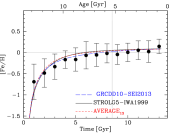
Figure 12: The age-metallicity relation, [Fe/H] vs time, for the average model constructed from the 13 selected models with $P_{j}=1$ as red line. The best model –labelled in the panel– obtained for this particular relation is the black line, almost indistinguishable. The model given by the maximum $P_{C}$ is the blue line. Dotted grey lines indicate the Sun position.

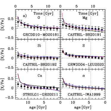
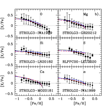
Figure 13: The relative abundances of [O/Fe], [Mg/Fe], [Si/Fe], [S/Fe], [Ca/Fe] and [$\alpha$/Fe] as a function of: a) the stellar age $\tau$ (in Gyr); b) the metallicity [Fe/H], for the average model constructed with the 13 selected models with $P_{j}=1$ as red line. The black line is the best model, as labelled in the panel, obtained for each particular relation [X/Fe]($\tau$) or [X/Fe]([Fe/H]). The model given by the maximum $P_{C}$ is the blue line. Dotted grey lines indicate the Sun position.

We now check if this mix of DTDs and SN-Ia yields may reproduce all sets of data. We show this resulting model in Fig. 12, and 13. In each one, we represent the best model for each relation given in Table 5, with a black line, the model given by the maximum $P_{C}$ with a blue line, and this model constructed as the average of the 13 best models as a red line, as labelled in Fig. 12. In Fig 13, we label only the best model for each data set, different for each panel, being the two other lines —blue and red— the same models for all panels. Sometimes the black and red lines are almost indistinguishable. In most of panels the average model reproduces the data better that the one given by $P_{C}$. Moreover, not all data are equally well fitted: Ca is not so flat with the age as data seems to indicate, which is the reason to have a high value $\chi^{2}_{min}=1.372$ compared with the others sets. Moreover, for Mg and Ca, models have peculiar behaviours compared with the data trends as we said, when represented as a function of [Fe/H] at the high-metallicity zone, since models decrease strongly at solar metallicity, in disagreement with observations that may be flatter from $\mbox{[Fe/H]}=0$. Globally, we do see a good correspondence for O, Si, S and $\alpha$, as a function of [Fe/H] and age.

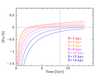
Figure 14: The age-metallicity relation [Fe/H] vs. time for different radial regions with colour lines as labelled, for the average model.

4.5 Results for other radial regions

The results from the average model for [X/Fe] relative abundances in other regions of the disc are analysed in this section. The age-metallicity relation is represented in Fig. 14. There is a clear dependence on the galactocentric distance, the inner regions showing higher metallicities than the outer ones, meaning that a negative radial gradient of metallicity, stronger in the past than now, appears in the disc.

In Fig. 15, we represent the evolution of [$\alpha$/Fe] as a function of the stellar age –left panels–and as a function of the metallicity [Fe/H] –right panels– for different radial regions of the disc, with same data –for the Solar Region–, as in previous figures. The most important point is the large dispersion shown in all $\alpha$-elements for the disc regions. This occurs for both types of relationships, either vs. age or vs. [Fe/H], although this is more relevant in the right panels. When data for the Solar Neighbourhood is compared with a model for a given galactocentric distance, it is not possible to explain the observed dispersion. As different regions of the disc do show different patterns in the plane [X/Fe], either vs. age or vs. [Fe/H], the observed dispersion would be an indicator of mixing of stars originally born in different radial regions.

4.6 Abundances dispersion

We have seen above that the relative abundance [X/Fe] data for the $\alpha$-elements show a large dispersion that any chemical evolution model may not reproduce with only one region. On the other hand, we have shown in the previous subsection 4.5 that model results for different radial regions may participate in the observed dispersion with variable contributions. In particular, we find a large dispersion among the disc regions results.

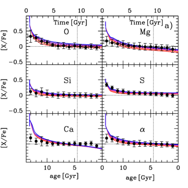
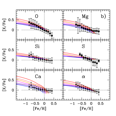
Figure 15: The relative abundances of [O/Fe], [Mg/Fe], [Si/Fe], [S/Fe], [Ca/Fe] and [$\alpha$/Fe] for the average model as a function of the stellar age (left panel) and of the metallicity (right panel) for different radial regions of the disc represented by different colour lines. The dots correspond to the binned data for the Solar Region.

In order to seek for a possible cause of the high dispersion in the observational data, we first look at the dispersion that the averaged model produce when all radial regions are included in the plot. This is shown in Fig.16, where we have the age-metallicity relation (top panels) and the relation [O/Fe] vs. [Fe/H] (bottom panels). Left panels show both relationships for all radial regions computed by the average model. In panel a) the dispersion shown by results is even higher than the observed one. In panel d), the dispersion of models is high at the early times/low metallicity regime, but it is smaller than shown by the data for [Fe/H]$>-1$. The fact that different radial regions show variable [Fe/H] and [O/Fe] is due to the SFR changing on radius in the disc, with higher rates in the early times for the inner regions, while in the outer regions the SFR starts with low values increasing with time. The data might correspond to objects born in other radial regions. Other explanation, besides this radial migration of stars, could include the uncertainties in the galactocentric distances.

The different DTDs or SN-Ia yields sets may also contribute to the dispersion. As said, there is no single model able to reproduce all observational data sets, and it has been necessary to mix some models to obtain one that may reproduce adequately all of them. It is, therefore, possible that some of these channels (DTDs or explosion mechanisms) that we have study here, appear simultaneolusly as SN Ia in a given region, more than one of them being valid. In that case, they would also create some data dispersion. We show in Fig. 16 the effect of including results for models with all DTDs and only one set of yields (IWA1999) for SN Ia (middle panels), and for models including all set of yields for SN Ia with only one DTD (STROLG3) (right panels) on the Solar region evolution. The variation of the DTDs appears around 3–5 Gyr. The effect of SN-Ia yields appears around 8–13 Gyr. A model with more than one DTD would show a dispersion similar to the observed one, while some simultaneous SN Ia yields sets do not produce so high variations. These results agree with Palla et al. (2022) findings, who by using [Mg/Fe] abundances from AMBRE-HARPS, and comparing them with detailed chemical evolution models, conclude that none set of yields may reproduce the data, even taken into account the stellar migration.

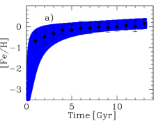
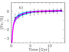
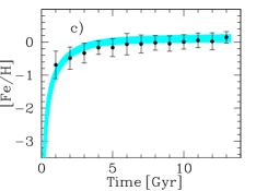
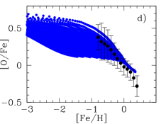
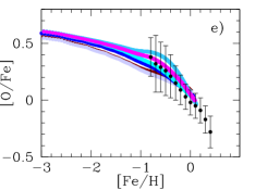
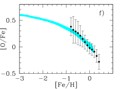
Figure 16: The age-metallicity relation and the relation [O/Fe] vs. [Fe/H] for all radial regions of the average model (left panels), and for the Solar Region with all DTDs and SN-Ia yields from GR20121 (middle panels), and for the STROLG3 DTD with all the SN-Ia yields (right panels).

5 Conclusions

We have studied the role of the different type Ia supernovae, mainly the different Delay Time Distribution (DTD) determined by the scenario of the binary systems and the yields of elements created by the different explosion mechanisms.

We have analysed carefully a large set of observations related with the $\alpha$-element over Iron abundances obtained from some modern surveys and other data of the literature. We have performed a binning of these data to obtain averaged values (see AppendixA, Supporting Information).

We have used an update of the MulChem chemical evolution model applied to the Milky Way Galaxy, where we have now taken the stellar yields from Cristallo et al. (2011, 2015) (the FRUITY set), for low and intermediate mass stars, and from Limongi & Chieffi (2018) for massive stars with several rotation stellar velocities. The calibration of the MWG model by using these stellar yields is given in Appendix B, Supporting Information.

To these prescriptions, we have added 15 possible DTDs for both DD and SD scenarios, and 12 sets of SNe Ia yields from recent works with different mechanisms of explosion. The combination of both inputs provide 180 different models, 148 of them considered realistic enough, although some of them are better than others, whose results have been compared with the binned data presented in the first part of work.

From this comparison, and after following a $\chi^{2}$-technique, we have found that no model may reproduce simultaneously the whole set of compiled data related to the age-metallicity relation, [Fe/H]$(t)$, and the relative abundances of $\alpha$-elements, [X/Fe], X being O, Mg, Ca, Si, S or an average $\alpha$, as a function of the stellar age or as a function of the metallicity [Fe/H]. We found the 13 best models able to reproduce each one of the 13 data sets with which we compare.

From these 13 best models, the most probable DTD is the one called STROLG3 from Strolger et al. (2020) with a delay of 350 Myr, although the data for the oldest stellar ages seem indicate the necessity of a delay as shorter as the one from Castrillo et al. (2021). The best set of SN-Ia yields seems to be IWA99 (MCh) followed by GR20211 (sub-MCh). Both combinations STROLG3 (SD) $+$ IWA99 or STROLG3$+$ GR20211, could indicate that the delayed detonation (DDT) and the double detonation (DDet) explosions be both the real channels for the SNIa and that a mix of the two would represent the observations. In fact, we have found that a average of the 13 best models is able to reproduce the whole observational points, being good enough to fit each data set separately. This model represents proportions of a 46% for each SD and DD scenario, and proportions 70%-30% for MCh and sub-MCh.

The dispersion given by chemical evolution models is high for different radial regions of the disc. This might suggest that the observed dispersion is related with uncertain distance determinations, or with the stellar migration in the disc. In our models, differences between radial regions are due to the SFR variations.

The data dispersion may be also explained by a mix of DTDs, that is of different scenarios to create SN Ia binary systems, or by a mix of explosions channels, although this do not produce a dispersion as high as DTDs. The observed dispersion is probably due to both effects: radial mixing and several simultaneous SN Ia scenarios/channels.

6 Data availability

1. The Appendix  A, Supporting Information in the publication, gives the whole description of the data, the normalization of different data sets, the binning process, and the tables of binned data.

2. The whole set of 180 models are available in electronic format upon request to the authors.

3. The DTD functions and the SN Ia yields are included in the package starmatrix, an Open Source Python code (Bazán & Mollá, 2022) that compute the new ejected elements by each SSP, (see https://github.com/xuanxu/starmatrix).

4. The calibration of the Galactic chemical evolution model is given in Appendix B, Supporting Information in the publication.

Appendix A Normalized and binned data

All the data used in this work come from different surveys as given in Table 1. The main point is that these abundances are given as [X/Y] $=\log{(X/Y)}-\log{(X/Y)_{\sun}}$, and obtained by using different solar abundances, as shown in Table 6. To compare all of them we need they be in a same scale. Therefore, we have re-normalized them to the same solar abundances scale from Lodders (2019).

Table 6: Solar reference abundances.

Reference*	Name	Solar$\dagger$	$\epsilon({\rm Fe})_{\sun}$	$\epsilon({\rm O})_{\sun}$	$\epsilon({\rm Mg})_{\sun}$	$\epsilon({\rm Si})_{\sun}$	$\epsilon({\rm S})_{\sun}$	$\epsilon({\rm Ca})_{\sun}$	$\epsilon({\rm C})_{\sun}$	$\epsilon({\rm N})_{\sun}$
(1)	CHEN00	A+09	7.50	8.69	7.60	7.51	–	6.34	–	–
(2)	GAIA-BER14	G+07	7.45	–	7.53	–	–	–	–	–
(3)	HYPATIA	L+09	7.46	8.73	7.54	7.53	7.16	6.31	8.39	7.86
(4)	HARPS-GTO	B+15	7.47	8.71, 8.65a	–	–	–	–	–	–
(5)	HARPS-GTO	S+00, A&G89	7.47b	–	–	–	–	–	–	8.05
(6)	HARPS-GTO	C+11, B+15	7.52c	8.71	–	–	–	–	–	–
(7)	HARPS-GTO	S+00, A&G89	7.47b	8.93	7.58	7.55	–	6.36	–	–
(10)	HARPS-GTO	S+00, A&G89	7.47b	–	–	–	7.21	–	–	–
(8)	GALAH	G+07	7.45	8.56	7.53	7.51	–	6.31	8.39	–
(11)	SANTOS20	G+07	7.45	–	7.53	–	–	–	–	–
–	–	L+19	7.54	8.82	7.61	7.60	7.24	6.36	8.56	7.94

After this, we have still seen differences in their scale, since we consider that all abundances [X/Fe] must be zero when the Iron abundance or metallicity [Fe/H]=0 and when the stellar age $\tau=5.4$ Gyr, that is, the data must be around the solar values in the solar metallicity and age. We have, therefore, analyzed each cloud of data for each set and element, to search for its center and then to shift it to locate it in the solar value.

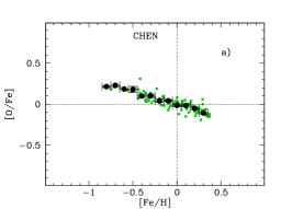
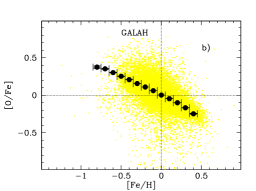
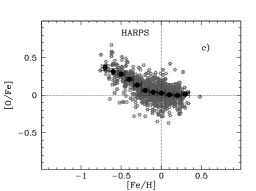
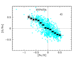
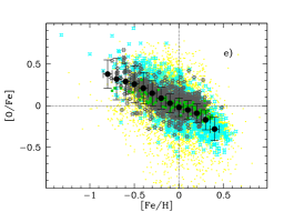
Figure 25: Binned data for [O/Fe] vs [Fe/H] from sets of different authors or surveys as labelled in panels a) to d). Panel e) shows all these data, over-plotted there are the joined binned dots.

In order to do this, we have selected the points around the solar age, radius or metallicity, in each case, and we have plotted the corresponding distribution [X/Fe] searching for the mean value by fitting a Gaussian. This averaged abundance must be in zero. This way ,we find the shift value $\Delta\,[X/Fe]_{shift}$ that we must apply to each set of data to put the cloud in the solar value. We show an example of the method in Fig. 17 with data from GALAH for [O/Fe]. There we see that the averaged [O/Fe]$\sim-0.10$ dex. Therefore, we move all GALAH [O/Fe] abundances adding +0.10 dex. Thus, the new abundances show the distributions of next Fig. 25, panel b). with the solar value in the middle of the distribution.

Table 7: Binned abundances of Iron [Fe/H] as a function of time, obtained from all set of data of Table 1 from main text.

Time	[Fe/H]
Gyr
1.00	-0.741 $\pm$ 0.416
2.00	-0.535 $\pm$ 0.336
3.00	-0.384 $\pm$ 0.299
4.00	-0.218 $\pm$ 0.207
5.00	-0.215 $\pm$ 0.275
6.00	-0.116 $\pm$ 0.321
7.00	-0.107 $\pm$ 0.271
8.00	-0.071 $\pm$ 0.225
9.00	-0.097 $\pm$ 0.234
10.00	-0.046 $\pm$ 0.217
11.00	0.003 $\pm$ 0.222
12.00	-0.028 $\pm$ 0.255
13.00	0.095 $\pm$ 0.171

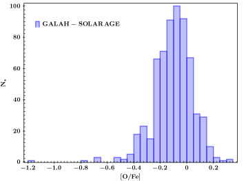
Figure 17: Distribution of the abundances [O/Fe] observed by GALAH with an averaged value <[O/Fe]>$\sim-0.10$ dex.

We have repeated this process for [Fe/H] and all relative abundances [X/Fe]. The resulting distributions are shown in Fig. 18 for [Fe/H] as a function of time, in Figures 20,  21,  22,  19,  23, and  24, for [X/Fe] as a function of the stellar age, and in Figs. 25,  26,  27,28,  29, and  30, as a function of metallicity [Fe/H]. In all of them we plot as dotted lines the Sun position, to check that each cloud of data has this position in the center.

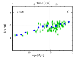
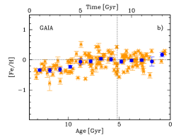
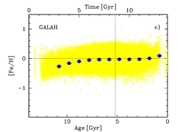
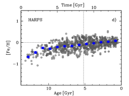
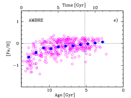
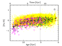
Figure 18: Binned data for [Fe/H] vs time from sets of different authors or surveys as labelled in panels a) to e). Panel f) shows all these data, over-plotted there are the joined binned dots.

Once obtained each distribution, we have binned each set, shown by the blue full dots. We have also plotted all sets together for each distribution in the last panel of each figure. In that case, the binned values represent the result of the binning process including all together the data coming from different surveys/authors (already being in the same scale). These last binned data are the ones used in the $\chi^{2}$-technique (see Section  4.3 of the main text) to compare models with observations.

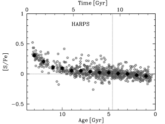
Figure 19: Binned data for [S/Fe] vs age in Gyr from HARPS survey. Only these data there exist for this element.

A.1 The age-metallicity relation

In this section, we show the data relative to the time evolution of the Iron abundance [Fe/H], usually taken as the measurement of the global metallicity, for the Solar Region. Data are taken from different surveys as given in Chen et al. (2000, CHEN), Bergemann et al. (2014, GAIA), Delgado Mena et al. (2015, 2017, HARPS), Buder et al. (2018, GALAH) and Santos-Peral et al. (2020, AMBRE). Fig. 18 shows 5 panels with data from CHEN, GAIA, GALAH, HARPS and AMBRE, and the last panel gives the binned points obtained from all survey data sets together. The resulting points of this binning are given in Table 7.

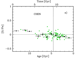
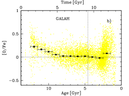
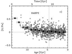
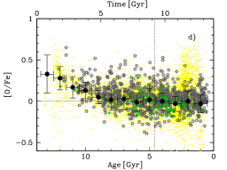
Figure 20: Binned data for [O/Fe] vs time or age in Gyr from sets of different authors or surveys as labelled in panels a) to c). Panel d) shows all these data, over-plotted there are the joined binned dots.

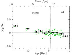
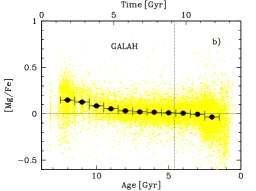
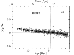
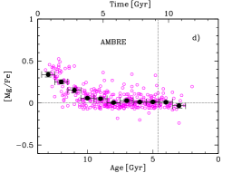
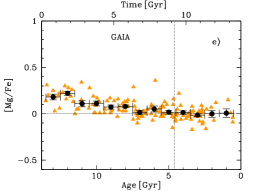
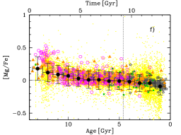
Figure 21: Binned data for [Mg/Fe] vs time or age in Gyr from sets of different authors or surveys as labelled in panels a) to e). Panel f) shows all these data, over-plotted there are the joined binned dots.

A.2 The evolution of the alpha-element abundances over the Iron along the stellar age

In this subsection we have obtained the relative abundances [X/Fe] for O, Mg, Si, S, Ca and $\alpha$ as a function of the stellar age, obtained for different methods by the different authors. Not all surveys have data for all the cited $\alpha$ -elements. Thus, we plot a figure for each element and each one has a different number of panels depending on the availability of data for this particular element in the studied surveys. Thus, In Fig 19, for [S/Fe], we have data only from HARPS.

For [O/Fe] vs $\tau$, we have data only from CHEN, GALAH and HARPS, and so we have three panels more the one corresponding to the binned data in Fig.20. For [Mg/Fe], Fig.21, however, there is 5 panels, (more the binned data one) since besides the three references cited, we also have data from GAIA and AMBRE. In the case of [Si/Fe] and [Ca/Fe] Fig 22, and Fig.23 we have again, as for [O/Fe], data from CHEN, GALAH and HARPS. For the global [$\alpha$/Fe] , data from CHEN, GALAH, HARPS and AMBRE are available.

The binned data obtained in the last panel of each figure is summarized in Table 8, where we give for each age in column 1, in Gyr, the corresponding [X/Fe] X being O, Mg, Si, S, Ca and global [$\alpha$], in columns 2, 3, 4, 5, 6, and 7.

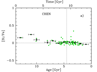
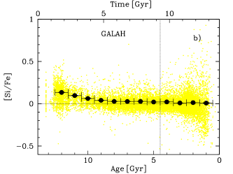
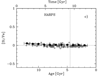
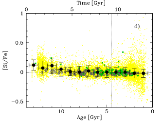
Figure 22: Binned data for [Si/Fe] vs time or age in Gyr from sets of different authors or surveys as labelled in panels a) to c). Panel d) shows all these data, over-plotted there are the joined binned dots.

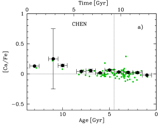
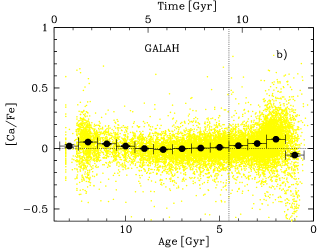
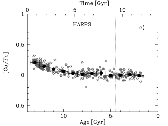
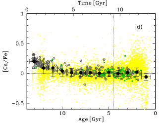
Figure 23: Binned data for [Ca/Fe] vs time or age from sets of different authors or surveys as labelled in panels a) to c). Panel d) shows all these data, over-plotted there are the joined binned dots.

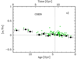
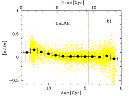
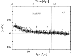
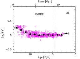
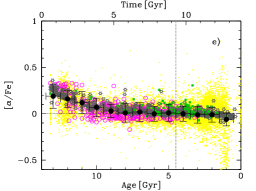
Figure 24: Binned data for [$\alpha$/Fe] vs time or age from sets of different authors or surveys as labelled in panels a) to d). Panel e) shows all these data, over-plotted there are the joined binned dots.

A.3 The evolution of the alpha-element abundances over the Iron as function of [Fe/H]

Finally, we show the available data for [X/Fe] as a function of the Iron abundance or metallicity [Fe/H]. In this case, it is easy to obtain observational data, since it is easy to estimate stellar abundances than stellar ages. We have, therefore, more panels in each figure. Thus, for [O/Fe] we hace CHEN, GALAH, HARPS, and HYPATIA data panels, as for [Si/Fe] and [Ca/Fe]. Instead, for [S/Fe] we have the HARPS data and furthermore the HYPATIA ones, with trends quite different. For [Mg/Fe] there are data for all surveys/references used: CHEN, GAIA, GALAH, HARPS, HYPATIA and AMBRE, while for [$\alpha$/fe] we have almost all, only GAIA do not give these data. In these data we note two facts: 1) there are stellar data for [Fe/H] higher than +0.1 dex, even until +0.5 dex, while in the age-metallicity relation, the metallicity do not arrive above this value. That means that it is possible to estimate so high metallicities but not their ages. Or that, maybe, the selection of the Solar region objects has been more precise in the case of [Fe/H](t); 2) The trend of these plots at high metallicity is sometime opposite between two different surveys: e.g.in [Mg/Fe] vs [Fe/H] there are points increasing after the solar value for high [Fe/H], while other show a trend of decreasing values. This same also occurs for other elements, too. (See Figures). The binned data obtained in the last panel of each figure is summarized in Table 9, where we give for each metallicity [Fe/H] in column 1, the corresponding [X/Fe] X being O, Mg, Si, S, Ca and global [$\alpha$], in columns 2, 3, 4, 5, 6, and 7.

Table 8: Binned abundances of alpha-elements over Iron, [X/Fe] as a function of the stellar age, obtained from all set of data of Table 1.

Age	[O/Fe]	[Mg/Fe]	[Si/Fe]	[S/Fe]	[Ca/Fe]	[$\alpha$/Fe]
(1)	(2)	(3)	(4)	. (5)	(6)	(7)
Gyr
1.00	-0.03 $\pm$ 0.06	-0.09$\pm$ 0.08	-0.02$\pm$ 0.02	-0.01$\pm$ 0.01	-0.06$\pm$ 0.01	-0.06$\pm$ 0.02
2.00	0.00 $\pm$ 0.07	-0.04$\pm$ 0.07	-0.02$\pm$ 0.03	0.01$\pm$ 0.01	0.02$\pm$ 0.02	-0.01$\pm$ 0.03
3.00	-0.03 $\pm$ 0.04	-0.04$\pm$ 0.08	0.00$\pm$ 0.03	0.03$\pm$ 0.01	0.01$\pm$ 0.01	-0.01$\pm$ 0.04
4.00	0.00 $\pm$ 0.05	-0.02$\pm$ 0.07	0.00$\pm$ 0.03	0.04$\pm$ 0.01	0.00$\pm$ 0.00	0.00$\pm$ 0.03
5.00	0.02 $\pm$ 0.08	-0.01$\pm$ 0.08	0.00$\pm$ 0.04	0.05$\pm$ 0.01	0.02$\pm$ 0.02	0.01$\pm$ 0.04
6.00	-0.01 $\pm$ 0.06	-0.01$\pm$ 0.09	0.00$\pm$ 0.03	0.06$\pm$ 0.01	0.00$\pm$ 0.01	0.00$\pm$ 0.03
7.00	0.03 $\pm$ 0.08	0.01$\pm$ 0.10	0.02$\pm$ 0.04	0.07$\pm$ 0.01	0.01$\pm$ 0.01	0.02$\pm$ 0.05
8.00	0.02 $\pm$ 0.08	0.01$\pm$ 0.08	0.00$\pm$ 0.05	0.08$\pm$ 0.01	0.01$\pm$ 0.01	0.01$\pm$ 0.05
9.00	0.05 $\pm$ 0.03	0.03$\pm$ 0.07	0.01$\pm$ 0.02	0.08$\pm$ 0.01	0.01$\pm$ 0.02	0.03$\pm$ 0.02
10.00	0.13 $\pm$ 0.05	0.07$\pm$ 0.10	0.05$\pm$ 0.07	0.13$\pm$ 0.02	0.04$\pm$ 0.05	0.07$\pm$ 0.05
11.00	0.17 $\pm$ 0.08	0.09$\pm$ 0.09	0.11$\pm$ 0.08	0.14$\pm$ 0.02	0.09$\pm$ 0.10	0.12$\pm$ 0.07
12.00	0.28 $\pm$ 0.09	0.12$\pm$ 0.09	0.07$\pm$ 0.07	0.24$\pm$ 0.01	0.09$\pm$ 0.05	0.16$\pm$ 0.04
13.00	0.33 $\pm$ 0.18	0.18$\pm$ 0.13	0.12$\pm$ 0.04	0.34$\pm$ 0.01	0.20$\pm$ 0.07	0.19$\pm$ 0.08

Table 9: Binned abundances of alpha-elements over Iron, [X/Fe] as a function of the Iron Abundances [Fe/H], obtained from all set of data of Table 1.

[Fe/H]	[O/Fe]	[Mg/Fe]	[Si/Fe]	[S/Fe]	[Ca/Fe]	[$\alpha$/Fe]
(1)	(2)	(3)	(4)	. (5)	(6)	(7)
-0.80	0.38 $\pm$ 0.12	0.27 $\pm$ 0.10	0.19$\pm$ 0.06	2000$\pm$ 0.00	0.14$\pm$ 0.08	0.28$\pm$ 0.07
-0.70	0.32 $\pm$ 0.20	0.22 $\pm$ 0.34	0.23$\pm$ 0.08	2000$\pm$ 0.00	0.22$\pm$ 0.10	0.23$\pm$ 0.12
-0.60	0.29 $\pm$ 0.17	0.22 $\pm$ 0.26	0.12$\pm$ 0.10	0.26$\pm$ 0.02	0.11$\pm$ 0.07	0.18$\pm$ 0.14
-0.50	0.26 $\pm$ 0.17	0.13 $\pm$ 0.14	0.05$\pm$ 0.06	0.20$\pm$ 0.02	0.10$\pm$ 0.06	0.14$\pm$ 0.08
-0.40	0.21 $\pm$ 0.14	0.09 $\pm$ 0.11	0.06$\pm$ 0.06	0.09$\pm$ 0.03	0.05$\pm$ 0.06	0.11$\pm$ 0.08
-0.30	0.15 $\pm$ 0.10	0.06 $\pm$ 0.09	0.01$\pm$ 0.06	0.09$\pm$ 0.06	0.04$\pm$ 0.04	0.08$\pm$ 0.06
-0.20	0.09 $\pm$ 0.08	0.03 $\pm$ 0.10	0.00$\pm$ 0.03	0.04$\pm$ 0.04	0.02$\pm$ 0.03	0.05$\pm$ 0.05
-0.10	0.03 $\pm$ 0.06	0.01 $\pm$ 0.07	-0.01$\pm$ 0.04	0.02$\pm$ 0.05	0.01$\pm$ 0.03	0.02$\pm$ 0.04
0.00	-0.02 $\pm$ 0.06	-0.01 $\pm$ 0.08	-0.03$\pm$ 0.05	-0.02$\pm$ 0.04	-0.01$\pm$ 0.03	0.00$\pm$ 0.04
0.10	-0.05 $\pm$ 0.06	-0.05 $\pm$ 0.07	-0.05$\pm$ 0.05	-0.12$\pm$ 0.13	-0.02$\pm$ 0.04	-0.02$\pm$ 0.03
0.20	-0.09 $\pm$ 0.06	-0.05 $\pm$ 0.07	-0.05$\pm$ 0.05	-0.13$\pm$ 0.13	-0.04$\pm$ 0.04	-0.05$\pm$ 0.03
0.30	-0.17 $\pm$ 0.07	-0.05 $\pm$ 0.09	-0.07$\pm$ 0.06	-0.18$\pm$ 0.16	-0.05$\pm$ 0.04	-0.07$\pm$ 0.05

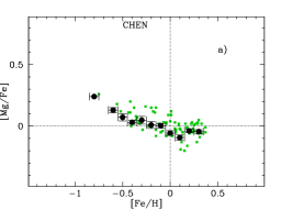
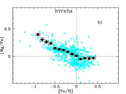
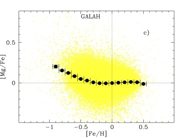
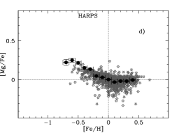
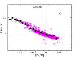
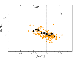
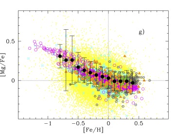
Figure 26: Binned data for [Mg/Fe] vs [Fe/H] from sets of different authors or surveys as labelled in panels a) to f). Panel g) shows all these data, over-plotted there are the joined binned dots.

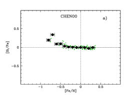
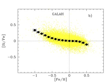
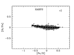
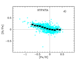
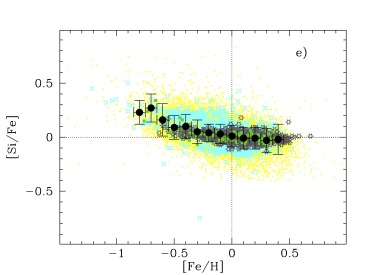
Figure 27: Binned data for [Si/Fe] vs [Fe/H] from sets of different authors or surveys as labelled in panels a) to d). Panel e) shows all these data, over-plotted there are the joined binned dots.

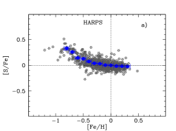
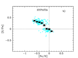
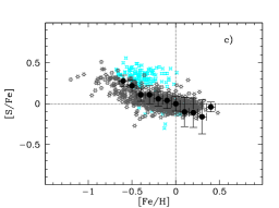
Figure 28: Binned data for [S/Fe] vs [Fe/H] from HARPS and HYPATIA surveys as labelled in panels a) and b). Panel c) shows all these data, over-plotted there are the joined binned dots.

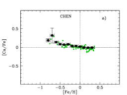
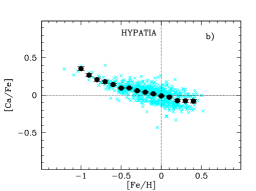
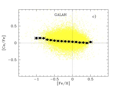
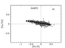
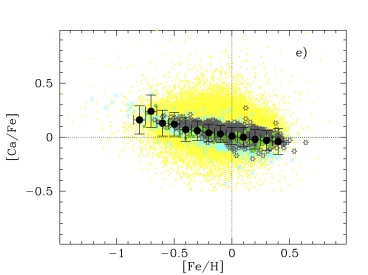
Figure 29: Binned data for [Ca/Fe] vs time from sets of different authors or surveys as labelled in panels a) to d). Panel e) shows all these data, over-plotted there are the joined binned dots.

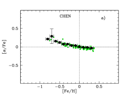
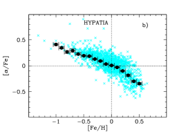
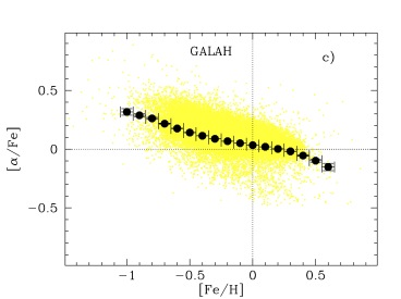
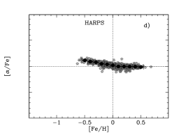
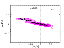
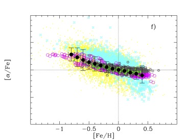
Figure 30: Binned data for [$\alpha$/Fe] vs [Fe/H] from sets of different authors or surveys as labelled in panels a) to e). Panel f) shows all these data, over-plotted there are the joined binned dots.

Appendix B Calibration of model for the Solar region and Galactic disc

B.1 The solar vicinity

In MOL15, a compilation of data from different authors (see references in that work) for MWG was presented. A binning process resulted in a set of binned data for each type of observation. This was described in detail in the Appendix from MOL15, where a table of references of these resulting binned distributions were given. The observational data basically included the solar neighbourhood time evolution of metallicity, SFR, and CNO abundances, in addition to the present state of the disc, including the radial distributions of surface densities for stars, gas, SFR, and CNO abundances.

In the present work, we adopted the data from references described in MOL15 for the solar vicinity time evolution of SFR. The data are binned for each Gyr with $\Delta t=\pm 0.5\,{\rm Gyr}$. The resulting SFR values were normalised to the most recent values of the SFR in the solar region at the present time, which was obtained as SFR${}_{\sun}\sim 0.266$ M_☉ yr^-1, at a galactocentric distance $R=8$ kpc.

The SFR and the C, N and O time evolution for the solar vicinity are plotted in Fig. 31 and Fig 32. In these figures all the 180 models give, as expected, similar results and are in agreement with the observational data obtained in MOL15. It is evident that these quantities do not dependent on the SN Ia rates nor on the SN Ia yields –much lower than the stellar yields from massive stars/CC SNs or from intermediate stars– shown in Fig. 5 of the main paper. Since we have updated the stellar yields for low and intermediate-mass stars, as well as massive stars, it is important to check that these new models still reproduce well the solar region observational data. We have checked that this is true by comparing the results for the 180 models –-which appear as only one—- with the data. In fact, we demonstrate that the star formation history (as the C, N and O abundances along the evolutionary time) shows good agreement compared with observational data, and effectively there is no change in the results depending on the DTD or on the SN Ia yield set.

B.2 The Galaxy disk

The data for radial distributions of surface densities in the MWG disc for HI, molecular gas, stellar profile and the SFR surface densities were taken from Table A3 in MOL15. The solar stellar surface density is between 33 and 64 $M_{\sun}$ pc^-2 from different authors. These values depend mostly on the scale length of the disc, $R_{\rm d}$, which is in the range [2.1–5.4] kpc. Therefore, we assume a certain uncertainty of $\sim 0.20$ dex in the absolute values of this radial distribution. The SFR binned radial distribution was also normalised to the SFR_☉. For what refers to the C, N and O abundances radial distributions, we have used the data of Table A4 from MOL15. In all cases, the error bars include the statistical error that corresponds to the dispersion of the original data coming from different authors, plus the systematical uncertainty due to the instrumental setup and to the techniques to estimate the final data from observations.

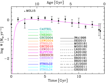
Figure 31: The SFR obtained for the solar vicinity (assumed at 8 kpc of galactocentric distance). Colours and line styles indicate different models (perfectly overlapping) as labelled in Tables 2 and 3 from the main paper. Black full dots represent the observational data compiled by Mollá et al. (2015, Appendix).

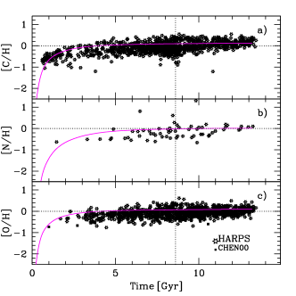
Figure 32: Time evolution of a) C; b) N; and c) O abundances, as [X/H] where the solar abundances are taken from Lodders (2019) for the complete set of models. Stellar abundance data are from Chen et al. (2000) and from the HARPS-GTO collaboration (see text for references). The dotted lines indicate the Sun position at its birth’s time, for reference. Different models are plotted as (overlapping) lines following the same style and colour scheme as in Fig. 31 although only a line is apparent since all models fall in the same locus.

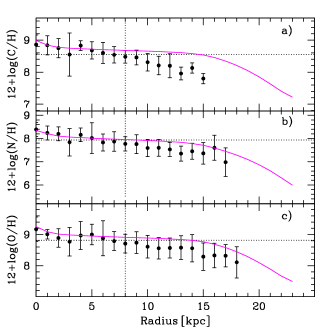
Figure 33: The radial distribution of elemental abundances of a) C; b) N; and c) O as $12+\log(\rm{X}/\rm{H})$, for the complete set of models. The black full dots are observational data taken from Mollá et al. (2015, Appendix). The dotted lines indicate the Sun abundance at its position $R=8.5$ kpc, for reference. Different models are plotted as (overlapping) lines following the same style and colour scheme as in Fig. 31 although only a line is apparent since all models fall in the same locus.

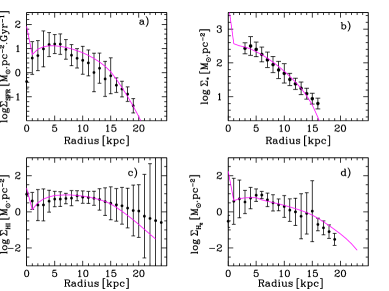
Figure 34: Radial densities distributions for the Galactic disc for the complete set of models. Panels correspond to: a) SFR; b) stellar mass; c) diffuse gas and d) molecular gas, all in units of M${}_{\sun}\,{\rm pc}^{-2}$, except for the SFR, which is in M${}_{\sun}\,{\rm pc}^{-2}\,{\rm Gyr}^{-1}$). Black full dots are binned data from Mollá et al. (2015, Appendix), while theoretical predictions are apparently shown with only a line because all models perfectly overlap in all panels.

Next figures refer to the radial distribution of different quantities throughout the Galactic disc. We show the radial distributions of C, N and O in Fig 33. Fig. 34 displays the surface density radial distributions of the SFR, the stellar profile, and both gas phases, diffuse and molecular. In all figures the corresponding data are those compiled in MOL15 with their error bars, which indicate the dispersion of the original data from different authors. In both figures, the results of all models are identical and the lines overlap each other. In all cases, the models still present satisfactory results in agreement with the observational data, taking into account the data spread and uncertainties.

We did not expect large differences between models for C, N and O, which basically come from stars of different masses, although there are small quantities coming from SN Ia. As explained above, we have included Fig. 32, and 31 as Fig. 33 and 34, to demonstrate that using different sets for stellar yields than MOL15 and MOL17 give essentially the same evolution for the Solar Region and the Galactic disc, that is, the new model is well calibrated compared with the data for these regions.

References

- Anders & Grevesse (1989) Anders E., Grevesse N., 1989, GeCoA, 53, 197
- Asplund et al. (2009) Asplund M., Grevesse N., Sauval A. J., Scott P., 2009, ARA&A, 47, 481
- Arcones & Thielemann (2023) Arcones A., Thielemann F.-K., 2023, A&ARv, 31, 1
- Aubourg et al. (2008) Aubourg É., Tojeiro R., Jimenez R., et al. 2008, A&A, 492, 631
- Barbary et al. (2012) Barbary K., et al., 2012, ApJ, 745, 32
- Bazán & Mollá (2022) Bazán J.J., Mollá M., Starmatrix: Modelling nucleosynthesis of galactic chemical elements. Journal of Open Source Software, 7(75), 4461, https://doi.org/10.21105/joss.04461.
- Bensby et al. (2014) Bensby T., Feltzing S., Oey M. S., 2014, A&A, 562, A71
- Bergemann et al. (2014) Bergemann M., et al., 2014, A&A, 565, A89
- Bertran de Lis et al. (2015) Bertran de Lis S., Delgado Mena E., Adibekyan V. Z., et al. , 2015, A&A, 576, A89
- Bildsten et al. (2007) Bildsten L., Shen K. J., Weinberg N. N., Nelemans G., 2007, ApJ, 662, L95
- Bours et al. (2013) Bours M. C. P., Toonen S., Nelemans G., 2013, A&A, 552, A24
- Bravo, Badenes, & Martínez-Rodríguez (2019) Bravo E., Badenes C., Martínez-Rodríguez H., 2019, MNRAS, 482, 4346
- Buder et al. (2018) Buder S., et al., 2018, MNRAS, 478, 4513
- Caffau et al. (2011) Caffau E., Ludwig H.-G., Steffen M., Freytag B., Bonifacio P., 2011, SoPh, 268, 255
- Calura et al. (2007) Calura F., Matteucci F., Tozzi P., 2007, MNRAS, 378, L11
- Carollo & Chiba (2021) Carollo D., Chiba M., 2021, ApJ, 908, 191
- Castrillo et al. (2021) Castrillo A., Ascasibar Y., Galbany L., et al. , 2021, MNRAS, 501, 3122
- Cavichia, Mollá, & Bazán (2023) Cavichia O., Mollá M., Bazán J. J., 2023, MNRAS, 520, 402
- Chabrier (2003) Chabrier G., 2003, ApJL, 586, L133
- Chen et al. (2000) Chen Y. Q., Nissen P. E., Zhao G., et al., 2000, A&AS, 141, 491
- Chen, Hu, & Wang (2021) Chen X., Hu L., Wang L., 2021, ApJ, 922, 15. doi:10.3847/1538-4357/ac178d
- Chiappini et al. (2011) Chiappini C., Frischknecht U., Meynet G., et al., 2011, Nature, 472, 454
- Costa Silva et al. (2020) Costa Silva A. R., Delgado Mena E., Tsantaki M., 2020, A&A, 634, A136
- Cristallo et al. (2011) Cristallo S., et al., 2011, ApJS, 197, 17
- Cristallo et al. (2015) Cristallo S., Straniero O., Piersanti L., Gobrecht D., 2015, ApJS, 219, 40
- De Donder & Vanbeveren (2004) De Donder E., Vanbeveren D., 2004, NewAR, 48, 861
- Delgado Mena et al. (2010) Delgado Mena E., Israelian G., González Hernández J. I., et al. 2010, ApJ, 725, 2349
- Delgado Mena et al. (2015) Delgado Mena E., et al., 2015, A&A, 576, A69
- Delgado Mena et al. (2017) Delgado Mena E., Tsantaki M., Adibekyan V. Z., Sousa S. G., 2017, A&A, 606, A94
- Delgado Mena et al. (2019) Delgado Mena E., et al., 2019, A&A, 624, A78
- de los Reyes et al. (2020) de los Reyes M. A. C., Kirby E. N., Seitenzahl I. R., Shen K. J., 2020, ApJ, 891, 85
- Di Stefano (2020) Di Stefano R., 2020, MNRAS, 493, 1855. doi:10.1093/mnras/staa220
- Doherty et al. (2017) Doherty C. L., Gil-Pons P., Siess L., Lattanzio J. C., 2017, PASA, 34, e056
- Eitner et al. (2020) Eitner P., Bergemann M., Hansen C. J., Cescutti G., et al., 2020, A&A, 635, A38
- Ferrini et al. (1992) Ferrini F., Matteucci F., Pardi C., Penco U., 1992, ApJ, 387, 138
- Ferrini et al. (1994) Ferrini F., Molla M., Pardi M. C., Diaz A. I., 1994, ApJ, 427, 745
- Flörs et al. (2020) Flörs A., et al., 2020, MNRAS, 491, 2902
- Friedmann & Maoz (2018) Friedmann M., Maoz D., 2018, MNRAS, 479, 3563
- Gilfanov & Bogdán (2010) Gilfanov M., Bogdán Á., 2010, Nature, 463, 924
- Goldstein & Kasen (2018) Goldstein D. A., Kasen D., 2018, ApJ, 852, L33
- Graur et al. (2011) Graur O., et al., 2011, MNRAS, 417, 916
- Graur & Maoz (2013) Graur O., Maoz D., 2013, MNRAS, 430, 1746
- Graur et al. (2017a) Graur O., Bianco F. B., Huang S., Modjaz M., et al. 2017a, ApJ, 837, 120X
- Graur et al. (2017) Graur O., Bianco F. B., Modjaz M., Shivvers I., Filippenko A. V., Li W., Smith N. et al., 2017, ApJ, 837, 121
- Greggio (2005) Greggio L., 2005, A&A, 441, 1055
- Greggio & Renzini (1983) Greggio L., Renzini A., 1983, A&A, 118, 217
- Grevesse, Asplund, & Sauval (2007) Grevesse N., Asplund M., Sauval A. J., 2007, SSRv, 130, 105
- Gronow et al. (2020) Gronow S., Collins C., Ohlmann S. T., Pakmor R., 2020, A&A, 635, A169
- Gronow et al. (2021) Gronow S., Côté B., Lach F., et al. , 2021, A&A, 656, A94
- Guillochon et al. (2010) Guillochon J., Dan M., Ramirez-Ruiz E., Rosswog S., 2010, ApJ, 709, L64
- Hachisu et al. (2008) Hachisu I., Kato M., Nomoto K., 2008, ApJ, 679, 1390
- Heringer et al. (2017) Heringer E., Pritchet C., Kezwer J. et al., 2017, ApJ, 834, 15
- Heringer et al. (2019) Heringer E., Pritchet C., van Kerkwijk M. H., 2019, ApJ, 882, 52
- (54) Hinkel N. R., Timmes F. X., Young P. A., Pagano M. D., et al. 2014, AJ, 148, 54
- Hitomi Collaboration et al. (2017) Hitomi Collaboration et al., 2017, Nature, 551, 478
- Howell et al. (2009) Howell D. A., et al., 2009, ApJ, 691, 661
- Iben & Tutukov (1984) Iben I. J., Tutukov A. V., 1984, ApJS, 54, 335
- Iwamoto et al. (1999) Iwamoto K., Brachwitz F., Nomoto K., et al. , 1999, ApJS, 125, 439
- Katz & Dong (2012) Katz B., Dong S., 2012, arXiv e-prints, arXiv:1211.4584
- Kobayashi & Nomoto (2009) Kobayashi C., Nomoto K., 2009, ApJ, 707, 1466
- Kobayashi, Leung, & Nomoto (2020) Kobayashi C., Leung S.-C., Nomoto K., 2020, ApJ, 895, 138. doi:10.3847/1538-4357/ab8e44
- Kromer et al. (2010) Kromer M., Sim S. A.,Fink M., Röpke F. K., 2010, ApJ, 719, 1067
- Kroupa (2001) Kroupa P., 2001, MNRAS, 322, 231
- Kuuttila et al. (2019) Kuuttila J., Gilfanov M., Seitenzahl I. R., et al., 2019, MNRAS, 484, 1317
- Lach et al. (2022) Lach F., Callan F. P., Bubeck D., et al., 2022, A&A, 658, A179
- Langer et al. (2000) Langer N., Deutschmann A., Wellstein S., Höflich P., 2000, A&A, 362, 1046
- Leung & Nomoto (2020) Leung S.-C., Nomoto K., 2020, ApJ, 888, 80.
- Leung & Nomoto (2018) Leung S.-C., Nomoto K., 2018, ApJ, 861, 143.
- Li et al. (2011a) Li W., et al., 2011a, MNRAS, 412, 1441
- Li et al. (2011b) Li W., Chornock R., Leaman J., Filippenko A. V., et al., 2011b, MNRAS, 412, 1473
- Limongi & Chieffi (2018) Limongi M., Chieffi A., 2018, ApJS, 237, 13
- Liu, Röpke, & Han (2023) Liu Z.-W., Röpke F. K., Han Z., 2023, RAA, 23, 082001
- Lodders, Palme, & Gail (2009) Lodders K., Palme H., Gail H.-P., 2009, LanB…4B, 4B, 712
- Lodders (2019) Lodders K., 2019, arXiv e-prints, arXiv:1912.00844
- Mannucci et al. (2005) Mannucci F., Della Valle M., Panagia N., Cappellaro E., et al., 2005, A&A, 433, 807
- Mannucci et al. (2006) Mannucci F., Della Valle M., Panagia N., 2006, MNRAS, 370, 773
- Mannucci (2009) Mannucci F., 2009, in Probing Stellar Populations out to the Distant Universe, American Institute of Physics Conference Series Vol. 1111, 467–476
- Maoz & Graur (2017) Maoz D., Graur O., 2017, ApJ, 848, 25
- Maoz et al. (2011) Maoz D., Mannucci F., Li W., et al., 2011, MNRAS, 412, 1508
- Maoz &Mannucci (2012b) Maoz D., Mannucci F., 2012, PASA, 29, 447
- Maoz et al. (2012a) Maoz D., Mannucci F., Brandt T. D., 2012, MNRAS, 426, 3282
- Maoz et al. (2014) Maoz D., Mannucci F., Nelemans G., 2014,ARA&A, 52, 107
- Maoz et al. (2010) Maoz D., Sharon K., Gal-Yam A., 2010, ApJ,722, 1879
- Matteucci & Greggio (1986) Matteucci F., Greggio L., 1986, A&A, 154, 279
- Matteucci et al. (2006) Matteucci F., Panagia N., Pipino A., et al., 2006, MNRAS, 372, 265
- Matteucci et al. (2009) Matteucci F., Spitoni E., Recchi S., Valiante R., 2009, A&A, 501, 531
- Mazzali et al. (2007) Mazzali P. A., Röpke F. K., Benetti S., Hillebrandt W., 2007, Sci, 315, 825
- Meng & Yang (2010) Meng X., Yang W., 2010, ApJ, 710, 1310
- Mennekens et al. (2010) Mennekens N., Vanbeveren D., De Greve J. P., De Donder E., 2010, 2010, A&A, 515, A89
- Mernier et al. (2016) Mernier F., et al., 2016, A&A, 595, A126
- Meynet et al. (2006) Meynet G., Ekström S., Maeder A., 2006, A&A, 447, 623
- Mollá & Díaz (2005) Mollá M., Díaz A. I., 2005, MNRAS, 358, 521
- Mollá et al. (2015) Mollá M., Cavichia O., Gavilán M., Gibson B. K., 2015, MNRAS, 451, 3693 (MOL15)
- Mollá et al. (2016) Mollá M., Díaz Á. I., Gibson B. K., et al., 2016, MNRAS, 462, 1329
- Mollá et al. (2017) Mollá M., Díaz Á. I., Ascasibar Y., Gibson B. K., 2017, MNRAS, 468, 305
- Mollá et al. (2019) Mollá M., Díaz Á. I., Cavichia O., Gibson B. K., et al., 2019, MNRAS, 482, 3071
- Mori et al. (2018) Mori K., Famiano M. A., Kajino T., et al., 2018, ApJ, 863, 176
- Nelemans et al. (2001) Nelemans G., Yungelson L. R., Portegies Zwart S. F., Verbunt F., 2001, A&A, 365, 491. doi:10.1051/0004-6361:20000147
- Nelemans, Toonen, & Bours (2013) Nelemans G., Toonen S., Bours M., 2013, IAUS, 281, 225
- Nomoto (1982) Nomoto K., 1982, ApJ, 257, 780
- Nomoto et al. (2013) Nomoto K., Kobayashi C., Tominaga N., 2013, ARA&A, 51, 457
- Nomoto & Leung (2019) Nomoto K., Leung S.-C., 2019, supe.book, 43
- Palla (2021) Palla M., 2021, MNRAS, 503, 3216
- Palla et al. (2022) Palla M., Santos-Peral P., Recio-Blanco A., Matteucci F., 2022, A&A, 663, A125
- Pakmor et al. (2013) Pakmor R., Kromer M., Taubenberger S., Springel V., 2013, ApJ, 770, L8
- Pakmor et al. (2022) Pakmor R., Callan F. P., Collins C. E., de Mink S. E., et al., 2022, MNRAS, 517, 5260. doi:10.1093/mnras/stac3107
- Piersanti et al. (2003) Piersanti L., Gagliardi S., Iben I., Tornambé A., 2003, ApJ, 598, 1229
- Portinari et al. (1998) Portinari L., Chiosi C., Bressan A., 1998, A&A, 334, 505
- Prantzos et al. (2018) Prantzos N., Abia C., Limongi M., et al., 2018, MNRAS, 476, 3432
- Raskin et al. (2009) Raskin C., Scannapieco E., Rhoads J., Della Valle M., 2009, ApJ, 707, 74
- Rodney et al. (2014) Rodney S. A., et al., 2014, AJ, 148, 13
- Ruiter et al. (2009) Ruiter A. J., Belczynski K., Fryer C., 2009, ApJ, 699, 2026
- Ruiter et al. (2011) Ruiter A. J., Belczynski K., Sim S. A., Hillebrandt W., Fryer C. L., Fink M., Kromer M. et al., 2011, MNRAS, 417, 408
- Ruiter (2020) Ruiter A. J., 2020, IAUS, 357, 1. doi:10.1017/S1743921320000587
- Ruiz-Lapuente, Canal, & Burkert (1997) Ruiz-Lapuente P., Canal R., & Burkert A., 1997, ASIC, 486, 205
- Ruiz-Lapuente et al. (2000) Ruiz-Lapuente P., Blinnikov S., Canal R., Mendez J., 2000, MmSAI, 71, 435
- Salpeter (1955) Salpeter E. E., 1955, ApJ, 121, 161
- Santos, Israelian, & Mayor (2000) Santos N. C., Israelian G., Mayor M., 2000, A&A, 363, 228
- Santos-Peral et al. (2020) Santos-Peral P., Recio-Blanco A., de Laverny P., et al., 2020, A&A, 639, A140
- Seitenzahl et al. (2013a) Seitenzahl I. R., et al., 2013a, MNRAS, 429, 1156
- Seitenzahl et al. (2013b) Seitenzahl I. R., Cescutti G., Röpke F. K., et al., 2013, A&A, 559, L5
- Shappee et al. (2013) Shappee B. J., Kochanek C. S., Stanek K. Z., 2013, ApJ, 765, 150
- Shen et al. (2018) Shen K. J., Kasen D., Miles B. J., Townsley D. M., 2018, ApJ, 854, 52
- Shivvers et al. (2017) Shivvers I., et al., 2017, PASP, 129, 054201
- Sim et al. (2013) Sim S. A., et al., 2013, MNRAS, 436, 333
- Smith et al. (2012) Smith M., et al., 2012, ApJ, 755, 61
- Strolger et al. (2020) Strolger L.-G., Rodney S. A., Pacifici C., et al., 2020, ApJ, 890, 140. doi:10.3847/1538-4357/ab6a97
- Soker (2019) Soker N., 2019, NewAR, 87, 101535. doi:10.1016/j.newar.2020.101535
- Suárez-Andrés et al. (2016) Suárez-Andrés L., Israelian G., González Hernández J. I., Adibekyan V. Z., et al., 2016, A&A, 591, A69
- Suárez-Andrés et al. (2017) Suárez-Andrés L., Israelian G., González Hernández J. I., Adibekyan V. Z., et al., 2017, A&A, 599, A96
- Sullivan et al. (2006) Sullivan M., et al., 2006, ApJ, 648, 868
- Talbot & Arnett (1973) Talbot Raymond J. J., Arnett W. D., 1973, ApJ, 186, 69
- Taubenberger (2017) Taubenberger S., 2017, hsn..book, 317
- Thomson & Chary (2011) Thomson M. G., Chary R. R., 2011, ApJ, 731, 72
- Tinsley (1979) Tinsley B. M., 1979, ApJ, 229, 1046
- Toonen et al. (2012) Toonen S., Nelemans G., Portegies Zwart S., 2012, A&A, 546, A70
- Totani et al. (2008) Totani T., Morokuma T., Oda T., Doi M., Yasuda N., 2008, PASJ, 60, 1327
- Tsujimoto & Shigeyama (2012) Tsujimoto T., Shigeyama T., 2012, ApJ, 760, L38
- Walcher et al. (2015) Walcher C. J., Coelho P. R. T., Gallazzi A., Bruzual G., et al., 2015, A&A, 582, A46
- Walcher et al. (2016a) Walcher C. J., et al., 2016, A&A, 594, A61
- Wang (2018) Wang B., 2018, RAA, 18, 049
- Weinberg et al. (2017) Weinberg D. H., Andrews B. H., Freudenburg J., 2017, ApJ, 837, 183
- Woosley & Kasen (2011) Woosley S. E., Kasen D., 2011, ApJ, 734, 38
- Yungelson & Livio (2000) Yungelson L. R., Livio M., 2000, ApJ, 528, 108