Robust Waveform Design for Integrated Sensing and Communication

Abstract

Integrated sensing and communication (ISAC), which enables hardware, resources (e.g., spectra), and waveforms sharing, is becoming a key feature in future-generation communication systems. This paper investigates robust waveform design for ISAC systems when the underlying true communication channels (e.g. time-selective ones) are not accurately known. With uncertainties in nominal communication channel models, the nominally-estimated communication performance may be not achievable in practice; i.e., the communication performance of ISAC systems cannot be guaranteed. Therefore, we formulate robust waveform design problems by studying the worst-case channels and prove that the robustly-estimated performance is guaranteed to be attainable in real-world operation. As a consequence, the reliability of ISAC systems in terms of communication performance is improved. The robust waveform design problems are shown to be non-convex, non-differentiable, and high-dimensional, which cannot be solved using existing optimization techniques. Therefore, we develop a computationally-efficient and globally-optimal algorithm to solve them. Simulation results show that the robustly-estimated communication performance can be ensured to be practically reachable while the nominally-estimated performance cannot, which validates the value of robust design.

I Introduction

Integrated sensing and communication (ISAC) is one of the enabling technologies for the sixth-generation (6G) communications. It uses one single hardware system to simultaneously realize the sensing and communication functions. This integration is able to improve spectral efficiency, reduce platform size, and control power consumption. From the signal processing perspective, one of the main features of ISAC is that the same transmitted waveform, called dual-functional waveform, is used for both sensing and communication functions [1, 2, 3, 4]. This paper is concerned with the problem of dual-functional waveform design for ISAC.

I-A Literature Review

Waveform design for ISAC aims to balance the performance for sensing and communication because an optimal waveform for sensing is not necessarily optimal for communication [3, 5], and vice versa. Typical performance measures for sensing include the Cramér–Rao bounds for the estimated parameters [3] and the sensing mutual information between received signals and sensing channels [6, 7], while those for communication include the distortion minimum mean-squared error [8] and the mutual information between the transmitted and the received signals (i.e., channel capacity) [3, 9]. In terms of designing methodology, the existing methods can be categorized into two main streams. The first stream directly works on designing the dual-functional waveforms by optimizing various performance measures [5, 10, 11], while the second stream focuses on finding the balanced waveforms for sensing and communication [12, 3, 4].

I-B Problem Statement

The existing design methods for ISAC waveforms face the following major drawback: In practice, the communication channel cannot be accurately known when designing waveforms. This point can be understood from three aspects. First, the communication channel is time-selective (i.e., time-varying). Second, the channel model used might be inexact. Third, any statistical method cannot give exact channel estimation when training samples are limited. In designing the optimal dual-functional waveforms, the actual performance of the nominally optimal waveforms may significantly degrade from the actually optimal performance if we use the estimated (i.e., nominal) communication-channel information as a surrogate of the true communication-channel information. Therefore, a robust dual-functional waveform design framework, which is insensitive to the modeling errors of the communication channel, is expected.

Related Works And Conceptual Novelty. Literature on robust dual-functional waveform design for ISAC is rather lacking. The only found record [13] is out of the technical scope of this paper. Other related works considering imperfect channel information include, e.g., robust precoding and beamforming [14, 15, 16, 17, 18].

I-C Contributions

As an illustration, this paper focuses on finding the balanced waveforms that are simultaneously close to the optimal waveforms for sensing and for communication. In this paper, the following contributions can be highlighted:

1. A robust dual-functional waveform design framework is proposed, which can hedge against the modeling errors of the communication channel, and hence improve the communication reliability of ISAC systems; see Problems (4) and (5), Fact 1, Fact 2, and Remark 3. The framework leverages the min-max formulation where the minimization of the objective is to design the optimal waveforms and the maximization of the objective is to find the worst-case information of the communication channel.

2. We show that the two-layer min-max formulation for dual-functional robust waveform design is equivalent to a single-layer maximization formulation, which is relatively easier to solve than the original min-max formulation; see Theorems 1 and 3.

3. Since the resulting maximization formulation is non-concave, non-convex, non-differentiable, and high-dimensional, a globally optimal solution framework is motivated and proposed; see Method 1, Proposition 5, and Theorem 2.

I-D Notation

Vectors (column by default) and matrices are denoted by bold symbols and are written in lowercase and uppercase letters, respectively; for example, $\bm{x}$ is a vector while $\bm{X}$ is a matrix. Deterministic quantities are denoted by Italic symbols (e.g., $\bm{x}$, $\bm{X}$) while random quantities are denoted by normal symbols (e.g., $\mathbf{x}$, $\mathbf{X}$). Sets are denoted by calligraphic symbols, e.g., $\mathcal{X}$. Let $\mathbb{C}^{d}$, $\mathbb{R}^{d}$ stand for a $d$-dimensional complex, real space, respectively. Let $\bm{X}^{\mathsf{T}}$, $\bm{X}^{\mathsf{H}}$, $\operatorname{Tr}[\bm{X}]$, $\|\bm{X}\|$, and $\bm{X}^{-1}$ denote the transpose, the conjugate transpose, the trace, a norm (e.g., the Frobenius norm $\|\bm{X}\|_{F}$), and the inverse of the matrix $\bm{X}$, respectively. When the inverse of $\bm{X}$ does not exist, we use $\bm{X}^{-1}$ to denote its Moore–Penrose pseudo-inverse. We use $\mathcal{CN}(\bm{0},\bm{\Sigma})$ to denote the circularly-symmetric complex normal distribution with zero mean, covariance matrix $\bm{\Sigma}$, and zero pseudo-covariance matrix. Let the running index set induced by an integer $I$ be denoted by $[I]\coloneqq\{1,2,\ldots,I\}$ and the $N$-dimensional identity matrix by $\bm{I}_{N}$.

II Problem Formulation And Model Analyses

Following the setups in [12], we consider a MIMO-based ISAC system with an $N$-antenna uniform linear array (ULA). The system simultaneously senses targets and communicates with $K$ single-antenna downlink users using shared dual-functional waveform $\bm{X}\in\mathbb{C}^{N\times L}$, where $L$ denotes the number of the communication frame (from the perspective of communication) and the number of snapshots (from the perspective of sensing). Letting $\bm{x}_{l}\in\mathbb{C}^{N}$ denote the transmitted $N$-dimensional signal vector for every $l\in[L]$, we have $\bm{X}\coloneqq[\bm{x}_{1},\bm{x}_{2},\ldots,\bm{x}_{l},\ldots,\bm{x}_{L}]$.

On the communication side, $\bm{X}$ is the output of pre-coding and conveys the information of communication symbols. For downlink communication with $K$ users, the base-band communication model is

$$\mathbf{Y}=\bm{H}\bm{X}+\mathbf{W},$$ (1)

where $\mathbf{Y}\in\mathbb{C}^{K\times L}$ denotes the received symbol matrix at all $K$ users, $\bm{H}\coloneqq[\bm{h}_{1},\bm{h}_{2},\ldots,\bm{h}_{K}]^{\mathsf{T}}\in\mathbb{C}^{K\times N}$ the communication channel matrix, and $\mathbf{W}\coloneqq[\mathbf{w}_{1},\mathbf{w}_{2},\ldots,\mathbf{w}_{L}]\in\mathbb{C}^{K\times L}$ the channel noise; for every $k\in[K]$, $\bm{h}_{k}$ denotes the channel model of the $k^{\text{th}}$ user; for every $l\in[L]$, $\mathbf{w}_{l}\sim\mathcal{CN}(\bm{0},N_{0}\bm{I}_{K})$ denotes the channel noise at the $l^{\text{th}}$ data unit and $N_{0}$ denotes the noise level. Note that given a waveform matrix $\bm{X}$ and a channel $\bm{H}$, the randomness of $\mathbf{Y}$ is from the randomness of $\mathbf{W}$. Suppose that the expected constellation-point matrix for the $K$ downlink users is $\bm{S}\in\mathbb{C}^{K\times L}$. We have the multi-user interference (MUI) signals $\bm{H}\bm{X}-\bm{S}$ and the total MUI energy can be calculated as $\|\bm{H}\bm{X}-\bm{S}\|^{2}_{F}$; see [12]. Therefore, from the perspective of communication, waveform design is to find a mapping $\mathcal{F}_{\bm{H}}:\bm{S}\to\bm{X}$ such that the total MUI energy $\|\bm{H}\cdot\mathcal{F}_{\bm{H}}(\bm{S})-\bm{S}\|^{2}_{F}$ is minimized, where $\mathcal{F}_{\bm{H}}$ depends on the communication channel information $\bm{H}$.

On the sensing side, the key is to design perfect beam patterns for target searching and/or tracking. According to [19], designing a beam pattern is equivalent to designing the cross-correlation matrix $\bm{R}\in\mathbb{C}^{N\times N}$ of the probing signals $\{\bm{x}_{l}\}$ for every $l\in[L]$. Therefore, from the perspective of sensing, waveform design is to find a mapping $\mathcal{F}:\bm{R}\to\bm{X}$ such that $\bm{X}\bm{X}^{\mathsf{H}}/L=\mathcal{F}(\bm{R})\mathcal{F}^{\mathsf{H}}(\bm{R})/L=\bm{R}$. For an omnidirectional beam pattern, $\bm{R}\coloneqq\frac{P_{\mathsf{T}}}{N}\bm{I}_{N}$ should be used, where $P_{\mathsf{T}}$ denotes the total transmitting power.

For an ISAC system, dual-functional waveform design can be stated as finding a mapping $\mathcal{F}_{\bm{H}}:(\bm{S},\bm{R})\to\bm{X}$ such that the total MUI energy $\|\bm{H}\cdot\mathcal{F}_{\bm{H}}(\bm{S},\bm{R})-\bm{S}\|^{2}_{F}$ is minimized and the cross-correlation matrix $\mathcal{F}_{\bm{H}}(\bm{S},\bm{R})\mathcal{F}^{\mathsf{H}}_{\bm{H}}(\bm{S},\bm{R})/L$ is as close as possible to the desired $\bm{R}$. In [12, Eq. (10)], the following sensing-centric ISAC waveform design problem is defined:

$$\begin{array}[]{cl}\displaystyle\min_{\bm{X}}&\|\bm{H}\bm{X}-\bm{S}\|^{2}_{F}\\ \text{s.t.}&\displaystyle\frac{1}{L}\bm{X}\bm{X}^{\mathsf{H}}=\bm{R},\end{array}$$ (2)

which aims to minimize the communication MUI energy while guaranteeing the perfect sensing performance. If we desire a balanced performance between communication and sensing, we can consider a joint design problem [12, Eq. (16)]:

$$\begin{array}[]{cl}\displaystyle\min_{\bm{X}}&\rho\|\bm{H}\bm{X}-\bm{S}\|^{2}_{F}+(1-\rho)\|\bm{X}-\bm{X}_{s}\|^{2}_{F}\\ \text{s.t.}&\displaystyle\frac{1}{L}\|\bm{X}\|^{2}_{F}=P_{\mathsf{T}},\end{array}$$ (3)

where $\bm{X}_{s}$ is a desired sensing waveform matrix (e.g., the optimal waveform for sensing regardless of communications), and $\rho\in[0,1]$ is the trade-off coefficient; $\bm{X}_{s}$ can also serve as a decision variable in (3) to further reduce the objective value, but we do not investigate this general case for computational efficiency. The constraint means that the total transmit power of the ISAC system is $P_{\mathsf{T}}$. As shown in [12, Fig. 3, Fig. 4], the waveform design criterion employing the total power constraint and the communication-sensing trade-off is more promising than that utilizing the per-antenna power constraint in terms of the higher average achievable sum rate (unit: bit-per-second/Hz) and the lower symbol-error rate. Therefore, the per-antenna power constraint is not investigated in this paper. Compared with (2), the hard constraint $\bm{X}\bm{X}^{\mathsf{H}}=L\bm{R}$ is relaxed to penalizing the mismatch $\bm{X}\bm{X}^{\mathsf{H}}-L\bm{R}$ in the objective and is further relaxed to penalizing the discrepancy $\bm{X}-\bm{X}_{s}$ in (3) due to technical tractability in developing the solution method, where $\bm{X}_{s}\bm{X}^{\mathsf{H}}_{s}=L\bm{R}$.

II-A Robust Waveform Design for ISAC

Considering the modeling errors in the communication channel $\bm{H}$, the following robust waveform design problem can be formulated

$$\begin{array}[]{cl}\displaystyle\min_{\bm{X}}\max_{\bm{H}}&\|\bm{H}\bm{X}-\bm{S}\|^{2}_{F}\\ \text{s.t.}&\displaystyle\frac{1}{L}\bm{X}\bm{X}^{\mathsf{H}}=\bm{R}\\ &\|\bm{H}-\bar{\bm{H}}\|\leq\theta,\end{array}$$ (4)

where $\bar{\bm{H}}$ is a nominal value (e.g., an estimate) of the true channel matrix, $\|\cdot\|$ denotes any suitable matrix norm (e.g., the Frobenius norm $\|\cdot\|_{F}$), and $\theta\geq 0$ is our trust level of the nominal $\bar{\bm{H}}$; the smaller the $\theta$, the more we trust $\bar{\bm{H}}$. Problem (4) is non-convex in $\bm{X}$ and non-concave in $\bm{H}$.

Similarly, another formulation for robust waveform design is

$$\begin{array}[]{cl}\displaystyle\min_{\bm{X}}\max_{\bm{H}}&\rho\|\bm{H}\bm{X}-\bm{S}\|^{2}_{F}+(1-\rho)\|\bm{X}-\bm{X}_{s}\|^{2}_{F}\\ \text{s.t.}&\displaystyle\frac{1}{L}\|\bm{X}\|^{2}_{F}=P_{\mathsf{T}}\\ &\|\bm{H}-\bar{\bm{H}}\|\leq\theta.\end{array}$$ (5)

Problem (5) is non-convex in $\bm{X}$ and non-concave in $\bm{H}$.

Related Works And Technical Novelty. From the viewpoint of optimization theory, the min-max formulations (4) and (5) are new and technically complicated in their own rights. In the authors’ knowledge, no literature working on similar optimization problems can be found. The only related one is [20], which somehow has a slight connection with (4), however, did not solve the same problem.

Remark 1 (Scalability of the Framework)

The extensions to the case of multi-antenna on the users’ side and the case of frequency-selective channels (e.g., orthogonal frequency-division multiplexing systems) are technically trivial, and hence, omitted in this paper. $\square$

Remark 2 (Specificity of Robust Formulations)

The mathematical forms of robust counterparts are specific to the adopted original (i.e., non-robust) waveform design frameworks since different waveform design philosophies give different waveform design formulations; cf. [2, 4]. This paper is, therefore, more or less tailored to the waveform design framework presented in [12]. $\square$

II-B Model Interpretation

Suppose the true communication channel is $\bm{H}_{0}$. According to (2), the problem that we really want to solve should be

$$\min_{\bm{X}:~{}\bm{X}\bm{X}^{\mathsf{H}}=L\bm{R}}\|\bm{H}_{0}\bm{X}-\bm{S}\|^{2}_{F}$$

which, however, cannot be conducted in practice because $\bm{H}_{0}$ is unknown. Therefore, a practical strategy is to find an upper bound $\mathcal{UB}(\bm{X})$ of the cost function $\|\bm{H}_{0}\bm{X}-\bm{S}\|^{2}_{F}$ for every $\bm{X}\in\mathcal{X}\coloneqq\{\bm{X}:\bm{X}\bm{X}^{\mathsf{H}}=L\bm{R}\}$ such that $\mathcal{UB}(\bm{X})$ is practically available. We assume that $\bm{H}_{0}$ is included in an uncertainty set $\{\bm{H}:~{}\|\bm{H}-\bar{\bm{H}}\|\leq\theta\}$ for some suitable matrix norm $\|\cdot\|$ where $\bar{\bm{H}}$ is an estimate of $\bm{H}_{0}$ and $\theta$ denotes the trust level. This assumption is practically reasonable because the estimate $\bar{\bm{H}}$ of the ground truth $\bm{H}_{0}$ can be close to $\bm{H}_{0}$. The fact below constructs an upper bound $\mathcal{UB}(\bm{X})$ of the cost function $\|\bm{H}_{0}\bm{X}-\bm{S}\|^{2}_{F}$ for every $\bm{X}\in\mathcal{X}$.

Fact 1 (Achievability of Robust Estimate)

Suppose $\bm{H}_{0}\in\mathcal{H}\coloneqq\{\bm{H}:~{}\|\bm{H}-\bar{\bm{H}}\|\leq\theta\}$. Then

$$\|\bm{H}_{0}\bm{X}-\bm{S}\|^{2}_{F}\leq\displaystyle\max_{\bm{H}\in\mathcal{H}}\|\bm{H}\bm{X}-\bm{S}\|^{2}_{F},~{}~{}~{}\forall\bm{X}\in\mathcal{X}.$$

Therefore, by minimizing the practically-available upper bound $\max_{\bm{H}\in\mathcal{H}}\|\bm{H}\bm{X}-\bm{S}\|^{2}_{F}$, we can also control the truly optimal cost $\min_{\bm{X}\in\mathcal{X}}\|\bm{H}_{0}\bm{X}-\bm{S}\|^{2}_{F}$ and the true cost $\|\bm{H}_{0}\bm{X}^{*}-\bm{S}\|^{2}_{F}$ of the waveform $\bm{X}^{*}$ because

$$\min_{\bm{X}\in\mathcal{X}}\|\bm{H}_{0}\bm{X}-\bm{S}\|^{2}_{F}\leq\|\bm{H}_{0}\bm{X}^{*}-\bm{S}\|^{2}_{F}\leq\|\bm{H}^{*}\bm{X}^{*}-\bm{S}\|^{2}_{F},$$

where $(\bm{X}^{*},\bm{H}^{*})\in\operatorname*{argmin}_{\bm{X}\in\mathcal{X}}\operatorname*{argmax}_{\bm{H}\in\mathcal{H}}\|\bm{H}\bm{X}-\bm{S}\|^{2}_{F}$ is a robust waveform and a worst-case channel. In other words, the robustly-estimated performance can always be achieved, even exceeded, in practice; NB: the smaller the MUI energies, the higher the communication performance. $\square$

Fact 1 explains the rationale of the robust waveform design model (4). The analysis on (5) is similar, and therefore, omitted. In contrast, the nominally optimal waveform(s) cannot provide such a performance guarantee.

Fact 2 (Unachievability of Nominal Estimate)

The nominally optimal cost cannot upper bound the truly optimal cost $\min_{\bm{X}\in\mathcal{X}}\|\bm{H}_{0}\bm{X}-\bm{S}\|^{2}_{F}$ and the true cost $\|\bm{H}_{0}\bar{\bm{X}}-\bm{S}\|^{2}_{F}$ of the waveform $\bar{\bm{X}}$ because

$$\min_{\bm{X}\in\mathcal{X}}\|\bm{H}_{0}\bm{X}-\bm{S}\|^{2}_{F}\leq\|\bm{H}_{0}\bar{\bm{X}}-\bm{S}\|^{2}_{F}\stackrel{{\scriptstyle\text{\scriptsize?}}}{{\leq}}\|\bar{\bm{H}}\bar{\bm{X}}-\bm{S}\|^{2}_{F},$$

where $\bar{\bm{X}}\in\operatorname*{argmin}_{\bm{X}\in\mathcal{X}}\|\bar{\bm{H}}\bm{X}-\bm{S}\|^{2}_{F}$ is a nominally optimal waveform and the symbol $\stackrel{{\scriptstyle\text{\scriptsize?}}}{{\leq}}$ means that the relation is not guaranteed. In other words, the nominally-estimated performance may not be achieved in practice. $\square$

The motivation and the necessity of the robust waveform design are summarized in the remark below.

Remark 3 (Benefit of Robust Waveform Design)

Suppose that $\bm{X}_{0}\in\min_{\bm{X}\in\mathcal{X}}\|\bm{H}_{0}\bm{X}-\bm{S}\|^{2}_{F}$ is a truly optimal waveform. In the practice of communications, finding the tight upper bound of the truly optimal cost $\|\bm{H}_{0}\bm{X}_{0}-\bm{S}\|^{2}_{F}$ and the true cost $\|\bm{H}_{0}\bm{X}-\bm{S}\|^{2}_{F}$ evaluated at the specified waveform $\bm{X}$ is critical. Suppose that an ISAC system can tolerate at most $C$ MUI energies for communications: i.e., for an employed waveform $\bm{X}^{\prime}$, we must have $\|\bm{H}_{0}\bm{X}^{\prime}-\bm{S}\|^{2}_{F}\leq C$. However, if we use the nominally optimal waveform $\bar{\bm{X}}$ designed at $\bar{\bm{H}}$, the designed nominally optimal cost $\|\bar{\bm{H}}\bar{\bm{X}}-\bm{S}\|^{2}_{F}\leq C$ does not necessarily imply the true cost $\|\bm{H}_{0}\bar{\bm{X}}-\bm{S}\|^{2}_{F}\leq C$. This may lead to significant dissatisfaction (i.e., bad user experiences) among communication users because the announced system performance $C$ cannot be guaranteed, and therefore, a serious reliability issue in communications arises. In contrast, if we employ the robust waveform design in (4), the dissatisfaction issue can be fixed; recall Fact 1. $\square$

Insight 1 (Uncertainty Quantification in Channel Estimation)

In practice, a satisfactory channel estimation method should therefore not only provide an estimate $\bar{\bm{H}}$ of the ground truth $\bm{H}_{0}$, but also provide the trust level $\theta$ with respect to the chosen norm $\|\cdot\|$. This basic statistical requirement, however, has not been seriously taken into account in trending channel estimation literature, especially for limited training data size (i.e. limited pilot length); see, e.g., [21, 22, 23]. $\square$

II-C Price of Robustness

As we can see, the robust design specifies an upper bound for the truly optimal cost and the true cost. In practice, however, this upper bound may be overly loose, i.e.,

$$\min_{\bm{X}\in\mathcal{X}}\|\bm{H}_{0}\bm{X}-\bm{S}\|^{2}_{F}\leq\|\bm{H}_{0}\bm{X}^{*}-\bm{S}\|^{2}_{F}\ll\|\bm{H}^{*}\bm{X}^{*}-\bm{S}\|^{2}_{F}.$$

To be specific, the robust waveform $\bm{X}^{*}$ that solves the min-max robust problem may induce a loose estimate of the truly optimal cost and the true cost, and therefore, the optimality of the solution is compromised. This raises the robustness-optimality tradeoff: to obtain robustness under uncertain conditions (i.e., when $\bm{H}_{0}$ is not exactly known), the price to pay is to sacrifice optimality under perfect conditions (i.e., when $\bm{H}_{0}$ is perfectly known).

II-D Budget of Uncertainty Set

To reduce the conservativeness of the robust design, a practical trick is to limit the size of the uncertainty set $\mathcal{H}$. To be specific, we employ a shrunken uncertainty set $\mathcal{H}_{\beta}\coloneqq\{\bm{H}:~{}\|\bm{H}-\bar{\bm{H}}\|\leq\beta\theta\}$ where $\beta\in[0,1]$ is the budget of the uncertainty set. Since

$$\min_{\bm{X}\in\mathcal{X}}\max_{\bm{H}\in\mathcal{H}_{\beta}}\|\bm{H}\bm{X}-\bm{S}\|^{2}_{F}\leq\min_{\bm{X}\in\mathcal{X}}\max_{\bm{H}\in\mathcal{H}}\|\bm{H}\bm{X}-\bm{S}\|^{2}_{F},$$

a tighter upper bound (i.e., the left-hand side of the above display) is suggested, which however cannot absolutely serve as an upper bound for the truly optimal cost and the true cost. The motivation is that in practice, $\bm{H}_{0}$ is still included in the shrunken set $\mathcal{H}_{\beta}$ with high probability. Nevertheless, the price is to meet the worst-case: $\bm{H}_{0}$ might be outside of $\mathcal{H}_{\beta}$. The fact below practically lifts Fact 1.

Fact 3 (Achievability in Probability)

If $\bm{H}_{0}$ is included in $\mathcal{H}_{\beta}$ with probability $\eta$ (e.g., $\eta=85\%$), then the robust cost $\min_{\bm{X}\in\mathcal{X}}\max_{\bm{H}\in\mathcal{H}_{\beta}}\|\bm{H}\bm{X}-\bm{S}\|^{2}_{F}$ upper bound the truly optimal cost and the true cost with probability $\eta$. $\square$

III Solution of Problem (4)

In this section, we find the solution of the problem (4). The solution of the problem (5) is to be investigated in the next section (Section IV).

III-A Model Reformulation

Since Problem (4) is non-convex in $\bm{X}$ and non-concave in $\bm{H}$, conventional solution methods (e.g., alternating descent, Lagrangian duality) for min-max problems are not applicable. However, Problem (4) can be equivalently transformed.

Theorem 1

Suppose that the beampattern-inducing matrix $\bm{R}$ is positive definite and $\bm{F}$ is invertible such that $\bm{R}=\bm{F}\bm{F}^{\mathsf{H}}$ (e.g., Cholesky decomposition). Then Problem (4) is equivalent to

$$\begin{array}[]{cl}\displaystyle\max_{\bm{H}}&\|\sqrt{L}\cdot\bm{H}\cdot\bm{F}\cdot\bm{U}\bm{I}_{N\times L}\bm{V}^{\mathsf{H}}-\bm{S}\|^{2}_{F}\\ \text{s.t.}&\|\bm{H}-\bar{\bm{H}}\|\leq\theta,\\ &\bm{U}\bm{\Sigma}\bm{V}^{\mathsf{H}}\overset{\text{SVD}}{=}\bm{F}^{\mathsf{H}}\bm{H}^{\mathsf{H}}\bm{S},\end{array}$$ (6)

where $\bm{U}\bm{\Sigma}\bm{V}^{\mathsf{H}}\overset{\text{SVD}}{=}\bm{F}^{\mathsf{H}}\bm{H}^{\mathsf{H}}\bm{S}$ means the singular value decomposition (SVD) of $\bm{F}^{\mathsf{H}}\bm{H}^{\mathsf{H}}\bm{S}$ and $\bm{I}_{N\times L}\coloneqq[\bm{I}_{N},\bm{0}_{N\times(L-N)}]$; the $N\times(L-N)$ zero matrix is denoted by $\bm{0}_{N\times(L-N)}$.

Proof:

See Appendix A, in which we construct saddle points for the original min-max problem (4). $\square$∎

Theorem 1 implies that the original two-layer min-max problem (4) can be equivalently solved by the single-layer maximization problem (6). The existence of such an equivalence stems from the existence of $\bm{X}^{*}_{\bm{H}}\in\operatorname*{argmin}_{\bm{X}:~{}\bm{X}\bm{X}^{\mathsf{H}}=L\bm{R}}\|\bm{H}\bm{X}-\bm{S}\|^{2}_{F}$ for every given $\bm{H}$. However, note that the solutions of (4) and (6) may not be unique.

III-B Property Analysis

In this subsection, we analyze the properties of the reformulated problem (6), which benefit the design of its solution method.

Denote the objective function and the feasible region in Problem (6) by

$$f(\bm{H})\coloneqq\|\sqrt{L}\cdot\bm{H}\cdot\bm{F}\cdot\bm{U}\bm{I}_{N\times L}\bm{V}^{\mathsf{H}}-\bm{S}\|^{2}_{F},$$ (7)

and

$$\mathcal{H}\coloneqq\{\bm{H}:~{}\|\bm{H}-\bar{\bm{H}}\|\leq\theta\},$$ (8)

respectively, where we suppress the dependence of $\mathcal{H}$ on $(\bar{\bm{H}},\theta,\|\cdot\|)$ to avoid notational clutter. Obviously, $\mathcal{H}$ is compact, i.e., closed and bounded.

The proposition below establishes the boundedness and the Lipschitz continuity of the function $f$ on $\mathcal{H}$.

Proposition 1

The function $f$ is bounded on $\mathcal{H}$ and $L_{f}$-Lipschitz continuous in $\bm{H}$ on $\mathcal{H}$ where

$$L_{f}=2BLP_{\mathsf{T}}\cdot(\|\bar{\bm{H}}\|_{F}+B\theta)+2B\sqrt{LP_{\mathsf{T}}}\cdot\|\bm{S}\|_{F}$$ (9)

and $B$ is a finite positive real number such that $\|\bm{H}\|_{F}\leq B\|\bm{H}\|$ for every $\bm{H}\in\mathcal{H}$.

Proof:

See Appendix B. $\square$∎

It is well believed that a Lipschitz continuous objective function is much easier to be globally maximized [24, p. 7]. An extreme case is that the Lipschitz constant is zero on $\mathcal{H}$ so the objective function $f$ is constant on $\mathcal{H}$. In this case, we just need to evaluate only one point on $\mathcal{H}$ to globally maximize $f$.

However, $f$ is non-differentiable, non-convex, and non-concave in $\bm{H}$ on $\mathcal{H}$, if $K\leq N\leq L$. The assumption $K\leq N\leq L$ is practical and natural; see, e.g., [25, Chap. 10] and [12, p. 4266].

Proposition 2

For the function $f(\bm{H})$ on $\mathcal{H}$, if $K\leq N\leq L$, then the following are true.

1. The function $f$ is non-differentiable with respect to $\bm{H}$.

2. The function $f$ is neither convex nor concave in $\bm{H}$.

Proof:

See Appendix C. $\square$∎

Nevertheless, the objective function $f(\bm{H})$ have tight and positive-definite quadratic (thus convex) upper bound $\overline{f}(\bm{H})$ and lower bound $\underline{f}(\bm{H})$.

Proposition 3

The function $f(\bm{H})$ is upper bounded by

$$\overline{f}(\bm{H})\coloneqq\|\bm{H}\bar{\bm{X}}-\bm{S}\|^{2}_{F}$$

and lower bounded by

$$\underline{f}(\bm{H})\coloneqq\Big{[}\sqrt{L\operatorname{Tr}[\bm{H}^{\mathsf{H}}\bm{H}\bm{R}]}-\|\bm{S}\|_{F}\Big{]}^{2}$$

for all possible $\bm{H}$, not necessarily on $\mathcal{H}$, where $\bar{\bm{X}}\coloneqq\sqrt{L}\bm{F}\bar{\bm{U}}\bm{I}_{N\times L}\bar{\bm{V}}^{\mathsf{H}}$, $\bar{\bm{U}}\bar{\bm{\Sigma}}\bar{\bm{V}}^{\mathsf{H}}\overset{\text{SVD}}{=}\bm{F}^{\mathsf{H}}\bar{\bm{H}}^{\mathsf{H}}\bm{S}$, and $\bar{\bm{H}}$ is the center of $\mathcal{H}$. In addition, the following are true.

1. The upper bound $\overline{f}(\bm{H})$ is positive-definite quadratic (thus convex) in $\operatorname{vec}(\bm{H})$.

2. The upper bound $\overline{f}(\bm{H})$ and the lower bound $\underline{f}(\bm{H})$ are both tight in the sense that the two bounds can be reached for some $\bm{H}$.

3. The upper bound $\overline{f}(\bm{H})$ has the same Lipschitz continuity constant $L_{f}$ as $f(\bm{H})$ on $\mathcal{H}$.

4. The difference between $\overline{f}(\bm{H})$ and $f(\bm{H})$ is uniformly bounded by $2L_{f}\cdot\theta$ on $\mathcal{H}$, i.e.,

   $$\overline{f}(\bm{H})-f(\bm{H})\leq 2L_{f}\cdot\theta.$$

   As a consequence, the positive-definite quadratic function $\overline{f}(\bm{H})-2L_{f}\cdot\theta$ is also a convex lower bound of $f(\bm{H})$ on $\mathcal{H}$: i.e., $\underline{f}(\bm{H})\coloneqq\overline{f}(\bm{H})-2L_{f}\cdot\theta$ is also a possible choice.

Proof:

See Appendix D. $\square$∎

Since the Lipschitz continuity constant in (9) is rather loose, the upper bound $2L_{f}\cdot\theta$ of the difference between $\bar{f}(\bm{H})$ and $f(\bm{H})$ can be much smaller in practice.

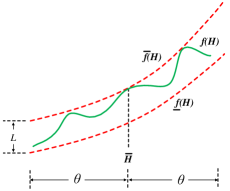
Propositions 2 and 3 suggest that the landscape of the objective function $f(\bm{H})$ is “globally positive-definite quadratic” but “locally non-convex, non-concave, and non-differentiable”. An illustration is shown in Fig. 1, in whose caption the implications from Propositions 2 and 3 are clarified.

Figure 1: An one-dimensional illustration of the landscape of the objective function $f(\bm{H})$ on $\mathcal{H}$. The upper bound and the lower bound of $f$ are $\overline{f}$ and $\underline{f}$, respectively; $\underline{f}\coloneqq\overline{f}-L$, where $L$ is the uniform gap between $\overline{f}$ and $\underline{f}$. Therefore, the upper bound $\overline{f}$ and the lower bound $\underline{f}$ are both positive-definite quadratic and thus convex. Note that $L\leq 2L_{f}\cdot\theta$. The center and the scale of the feasible region $\mathcal{H}$ are $\bar{\bm{H}}$ and $\theta$, respectively. At the center $\bar{\bm{H}}$, $f(\bar{\bm{H}})$ reaches its upper bound $\overline{f}(\bar{\bm{H}})$. Since the three functions $f$, $\overline{f}$, and $\underline{f}$ share the same Lipschitz continuity constant, the objective function $f$ cannot be overly rugged (i.e., it is relatively flat) in between the two bounds $\overline{f}$ and $\underline{f}$. Note that $f$ is non-differentiable on $\mathcal{H}$.

In consideration of the landscape and other properties (i.e., non-convexity, non-concavity, non-differentiability, Lipschitz continuity, etc.) of the objective function $f(\bm{H})$ in Problem (6), the zero-order optimization methods such as heuristic optimization [26, 27, 28, 29], Bayesian optimization [30, 31, 32], etc., are the last possible choices. However, a zero-order method is globally optimal for continuous objective functions if and only if the evaluation points governed by the searching algorithm are dense in the feasible region [33]. However, the searching space of Problem (6) is extremely large; when the number $K$ of communication users and the number $N$ of transmit antennas are large, the dimension of $\bm{H}$ will be large because $\bm{H}\in\mathbb{C}^{K\times N}$. Recall that for large-scale MIMO of 5G and 6G communications, the antenna number $N$ is expected to be large [34]. To be specific, there are in total $2KN$ real numbers involved. Even if we only query $I$ points in each dimension, we must evaluate the function $f(\bm{H})$ at least $I^{2KN}$ times to ensure global optimality for Problem (6). This is a well-identified dilemma known as “the curse of dimensionality” in global optimization; for rigorous complexity results in numerical accuracy and numerical computation, see, e.g., [24, p. 10], [35], [36, Table 1].

In summary, Problem (6) has almost all the unwanted properties that we can imagine for a global optimization problem: large dimensionality, non-differentiability, non-convexity, and non-concavity. Therefore, an ad-hoc and efficient algorithm solving Problem (6) is to be designed.

III-C Solution Method

In Sub-subsection III-C1, we derive the solution method and in Sub-subsection III-C2, we present an intuitive understanding of the developed method.

III-C1 Technical Development

By introducing auxiliary variables $\bm{A}$, $\bm{U}$, $\bm{\Sigma}$, and $\bm{V}$, we consider an optimization equivalent of Problem (6):

$$\begin{array}[]{cl}\displaystyle\max_{\bm{H},\bm{A},\bm{U},\bm{\Sigma},\bm{V}}&\|\sqrt{L}\bm{H}\bm{F}\bm{A}-\bm{S}\|^{2}_{F}\\ \text{s.t.}&\|\bm{H}-\bar{\bm{H}}\|\leq\theta,~{}~{}\bm{U}\bm{\Sigma}\bm{V}^{\mathsf{H}}=\bm{F}^{\mathsf{H}}\bm{H}^{\mathsf{H}}\bm{S},\\ &\bm{A}=\bm{U}\bm{I}_{N\times L}\bm{V}^{\mathsf{H}},~{}\bm{U}\bm{U}^{\mathsf{H}}=\bm{I}_{N},~{}\bm{V}\bm{V}^{\mathsf{H}}=\bm{I}_{L},\\ &\bm{\Sigma}\text{~{}is diagonal, non-negative, and real}.\end{array}$$ (10)

Recall from Theorem 1 that for every given $\bm{H}$, the corresponding optimal waveform $\bm{X}^{*}_{\bm{H}}=\sqrt{L}\bm{F}\bm{A}$. In terms of the variables $\bm{U}$, $\bm{\Sigma}$, and $\bm{V}$, the transformed problem (10) is just a feasibility problem because the three variables are not involved in the objective function. Since the rank of the matrix $\bm{F}^{\mathsf{H}}\bm{H}^{\mathsf{H}}\bm{S}$ is no larger than $K$ where $K\leq N\leq L$, the SVD of $\bm{F}^{\mathsf{H}}\bm{H}^{\mathsf{H}}\bm{S}$ is not unique for every feasible $\bm{H}$; to be specific, the feasible values of $\bm{U}$ and $\bm{V}$ are not unique. As a result, the feasible value of $\bm{A}$ is also not unique given $\bm{H}$.

In terms of the variable $\bm{H}$, the vectorized optimization equivalent of (10) is

$$\begin{array}[]{cl}\displaystyle\max_{\bm{H}}\max_{\bm{A},\bm{U},\bm{\Sigma},\bm{V}}&\|\sqrt{L}((\bm{F}\bm{A})^{\mathsf{T}}\otimes\bm{I}_{K})\operatorname{vec}(\bm{H})-\operatorname{vec}(\bm{S})\|^{2}_{2}\\ \text{s.t.}&(\bm{F}^{\mathsf{T}}\otimes\bm{S}^{\mathsf{H}})\operatorname{vec}(\bm{H})=\operatorname{vec}(\bm{V}\bm{\Sigma}^{\mathsf{H}}\bm{U}^{\mathsf{H}}),\\ &\|\operatorname{vec}(\bm{H})-\operatorname{vec}(\bar{\bm{H}})\|\leq\theta,\\ &\bm{A}=\bm{U}\bm{I}_{N\times L}\bm{V}^{\mathsf{H}},\\ &\bm{U}\bm{U}^{\mathsf{H}}=\bm{I}_{N},~{}\bm{V}\bm{V}^{\mathsf{H}}=\bm{I}_{L},\\ &\bm{\Sigma}\text{~{}is diagonal, non-negative, and real}.\end{array}$$ (11)

The key properties of the problem (11) are given below.

Proposition 4

Consider the reformulated problem (11). The following is true.

1. The objective function is positive-definite quadratic in $\operatorname{vec}(\bm{H})$.

2. In terms of both $\bm{H}$ and $\bm{A}$, the objective function is convex, and the constraints are also convex.

Proof:

See Appendix E. $\square$∎

To obtain an elegant solution, we impose an additional constraint $\bm{U}\bm{I}_{N\times L}\bm{V}^{\mathsf{H}}=\bar{\bm{U}}\bm{I}_{N\times L}\bar{\bm{V}}^{\mathsf{H}}$ on the original problem (11) to limit the size and shape of the feasible region of $\bm{H}$, and thus, simplify the problem. Intuitively speaking, this strategy is to let the nominally optimal solution $\bar{\bm{X}}$ simultaneously solve the robust problem: i.e., $\max_{\bm{H}}\min_{\bm{X}}\|\bm{H}\bm{X}-\bm{S}\|^{2}_{F}=\max_{\bm{H}}\|\bm{H}\bar{\bm{X}}-\bm{S}\|^{2}_{F}$, through which the relation of $\bm{X}^{*}=\bar{\bm{X}}$ can be guaranteed; note that $\bar{\bm{X}}=\sqrt{L}\bm{F}\bar{\bm{A}}=\sqrt{L}\bm{F}\bar{\bm{U}}\bm{I}_{N\times L}\bar{\bm{V}}^{\mathsf{H}}$. This is a practical trick to reduce the complexity of the original problem (11), which however does not violate the principle of robust waveform design in Fact 1; recall the optimality in the sense of bounding of the truly optimal cost and the true cost. We do not directly consider the constraint $\sqrt{L}\bm{F}\bm{U}\bm{I}_{N\times L}\bm{V}^{\mathsf{H}}=\bar{\bm{X}}$ because $\bm{F}$ is invertible, and therefore, the two means are equivalent. The method below formalizes the above reasoning.

Method 1

Suppose a SVD of $\bm{F}^{\mathsf{H}}\bar{\bm{H}}^{\mathsf{H}}\bm{S}$ is $\bar{\bm{U}}\bar{\bm{\Sigma}}\bar{\bm{V}}^{\mathsf{H}}\overset{\text{SVD}}{=}\bm{F}^{\mathsf{H}}\bar{\bm{H}}^{\mathsf{H}}\bm{S}$. Let $\bar{\bm{A}}\coloneqq\bar{\bm{U}}\bm{I}_{N\times L}\bar{\bm{V}}^{\mathsf{H}}$. If we consider $\bm{U}$ and $\bm{V}$ such that $\bm{U}\bm{\Sigma}\bm{V}^{\mathsf{H}}\overset{\text{SVD}}{=}\bm{F}^{\mathsf{H}}\bm{H}^{\mathsf{H}}\bm{S}$ and $\bm{U}\bm{I}_{N\times L}\bm{V}^{\mathsf{H}}=\bar{\bm{U}}\bm{I}_{N\times L}\bar{\bm{V}}^{\mathsf{H}}$, then the problem (11) is globally solved by $(\bm{H}^{*},\bar{\bm{A}},{\bm{U}}^{*},\bm{\Sigma}^{*},{\bm{V}}^{*})$ where $\bm{H}^{*}$ is a global maximum of the upper bound function $\overline{f}(\bm{H})$

$$\begin{array}[]{cl}\displaystyle\max_{\bm{H}}&\|\sqrt{L}((\bm{F}\bar{\bm{A}})^{\mathsf{T}}\otimes\bm{I}_{K})\operatorname{vec}(\bm{H})-\operatorname{vec}(\bm{S})\|^{2}_{2}\\ \text{s.t.}&\|\operatorname{vec}(\bm{H})-\operatorname{vec}(\bar{\bm{H}})\|\leq\theta,\end{array}$$ (12)

and $({\bm{U}}^{*},\bm{\Sigma}^{*},{\bm{V}}^{*})$ is a global minimum of the remedy problem, i.e.,

$$\begin{array}[]{cl}\displaystyle\min_{\bm{U},\bm{\Sigma},\bm{V}}&\alpha\|\bm{U}\bm{\Sigma}\bm{V}^{\mathsf{H}}-\bm{F}^{\mathsf{H}}\bm{H}^{*\mathsf{H}}\bm{S}\|^{2}_{F}+\|\bm{U}\bm{I}_{N\times L}\bm{V}^{\mathsf{H}}-\bar{\bm{A}}\|^{2}_{F}\\ \text{s.t.}&\bm{U}\bm{U}^{\mathsf{H}}=\bm{I}_{N},~{}\bm{V}\bm{V}^{\mathsf{H}}=\bm{I}_{L},\\ &\bm{\Sigma}\text{~{}is diagonal, non-negative, and real},\end{array}$$ (13)

where $\alpha\geq 0$ is a large real number to ensure that $\bm{U}\bm{\Sigma}\bm{V}^{\mathsf{H}}$ is a SVD of $\bm{F}^{\mathsf{H}}\bm{H}^{*\mathsf{H}}\bm{S}$. The solution $(\bm{H}^{*},\bar{\bm{A}},{\bm{U}}^{*},\bm{\Sigma}^{*},{\bm{V}}^{*})$ is globally optimal to Problem (6) in the sense of robust design in Fact 1, i.e., upper bounding the truly optimal cost, the true cost, and the nominally optimal cost; for intuitive algorithmic insights of Method 1, see Subsection III-C2. $\square$

In Method 1, by employing a trade-off coefficient $\alpha$, the exact equality of $\bm{U}\bm{I}_{N\times L}\bm{V}^{\mathsf{H}}=\bar{\bm{A}}=\bar{\bm{U}}\bm{I}_{N\times L}\bar{\bm{V}}^{\mathsf{H}}$ is compromised. To be specific, we relax the hard constraint $\bm{U}\bm{I}_{N\times L}\bm{V}^{\mathsf{H}}=\bar{\bm{A}}$. As in (13), we just require $\bm{U}\bm{I}_{N\times L}\bm{V}^{\mathsf{H}}$ to be as close as possible to $\bar{\bm{A}}$. This is a practical trick to reduce the technical complexity when minimizing over $\bm{U}$, $\bm{\Sigma}$, and $\bm{V}$. Another minor consideration is that the values of $\bm{U}$ and $\bm{V}$ that strictly satisfy $\bm{U}\bm{I}_{N\times L}\bm{V}^{\mathsf{H}}=\bar{\bm{A}}$ might not exist for every specified $\bm{H}$; some technical regularization conditions are needed to ensure the existence. However, if we use the soft-constraint counterpart as in (13), we do not need to explicitly derive the regularization conditions; this leads to $\bm{X}^{*}\approx\bar{\bm{X}}$.

As a result, the key is to solve the two sub-problems (12) and (13). Since the problem (12) is not convex, it is not straightforward to solve. Nevertheless, Problem (12) has nice properties to benefit the design of a globally optimal algorithm: it is positive-definite quadratic in $\operatorname{vec}(\bm{H})$ and has convex constraints for $\operatorname{vec}(\bm{H})$. We rewrite (12) in real spaces in a compact form:

$$\begin{array}[]{cl}\displaystyle\max_{\bm{h}\in\mathbb{R}^{2KN}}\|\bm{C}\bm{h}-\bm{s}\|^{2}_{2},~{}~{}\text{s.t.}~{}~{}\|\bm{h}-\bar{\bm{h}}\|\leq\theta,\end{array}$$ (14)

where $\bm{h}\coloneqq[\operatorname{real}^{\mathsf{T}}(\operatorname{vec}(\bm{H})),~{}\operatorname{imag}^{\mathsf{T}}(\operatorname{vec}(\bm{H}))]^{\mathsf{T}}\in\mathbb{R}^{2KN}$ is a real-valued vector constructed by stacking its real and imaginary components; the quantities $\bm{C}\in\mathbb{R}^{2KL\times 2KN}$, ${\bm{s}}\in\mathbb{R}^{2KL}$, and $\bar{\bm{h}}\in\mathbb{R}^{2KN}$ are constructed from (12) in a similar way, during which the lemma below is useful.

Lemma 1

Suppose $\bm{\Xi}\coloneqq\bm{\Gamma}+\bm{\Theta}j$ and $\bm{\xi}\coloneqq\bm{\alpha}+\bm{\beta}j$ where $j$ denotes the imaginary unit; $\bm{\Gamma}$ and $\bm{\Theta}$ are real matrices and $\bm{\alpha}$ and $\bm{\beta}$ are real vectors. We have

$$\left[\begin{array}[]{cc}\operatorname{real}(\bm{\Xi}\bm{\xi})\\ \operatorname{imag}(\bm{\Xi}\bm{\xi})\end{array}\right]=\left[\begin{array}[]{cc}\bm{\Gamma}&-\bm{\Theta}\\ \bm{\Theta}&\bm{\Gamma}\end{array}\right]\left[\begin{array}[]{c}\bm{\alpha}\\ \bm{\beta}\end{array}\right].$$

Proof:

We have $(\bm{\Gamma}+\bm{\Theta}j)(\bm{\alpha}+\bm{\beta}j)=(\bm{\Gamma}\bm{\alpha}-\bm{\Theta}\bm{\beta})+(\bm{\Theta}\bm{\alpha}+\bm{\Gamma}\bm{\beta})j$. Hence, the stacking scheme to construct real quantities from complex quantities is given in the statement of the lemma. This completes the proof. $\square$∎

Let the objective function of (14) be $p(\bm{h})$. We can further show that $p(\bm{h})$ is positive-definite and strongly convex.

Corollary 1

The objective function $p(\bm{h})$ of (14) is positive definite and strongly convex in $\bm{h}$.

Proof:

See Appendix F. $\square$∎

Equipped with Corollary 1, Proposition 5 below generates the globally optimal solution(s) to Problem (14), and hence, to Problem (12).

Proposition 5 (Solution of Upper-Bound Problem (14))

The globally optimal solution of the upper-bound problem (14), and therefore of Problem (12), is given by the following algorithmic iteration process.

1. Initialization: Let the iteration count $k=0$. Choose $\bm{h}_{0}$ from the domain $\{\bm{h}:~{}\|\bm{h}-\bar{\bm{h}}\|\leq\theta\}$ but $\bm{h}_{0}\neq(\bm{C}^{\mathsf{T}}\bm{C})^{-1}\bm{C}^{\mathsf{T}}\bm{s}$.

2. Solve

   $$\begin{array}[]{ccl}\bm{y}_{k}=&\displaystyle\operatorname*{argmax}_{\bm{y}\in\mathbb{R}^{2KN}}&(-\bm{s}^{\mathsf{T}}\bm{C}+\bm{h}^{\mathsf{T}}_{k-1}\bm{C}^{\mathsf{T}}\bm{C})\cdot\bm{y}\\ &\text{s.t.}&\|\bm{C}\bm{y}-\bm{s}\|^{2}_{2}=\|\bm{C}\bm{h}_{k-1}-\bm{s}\|^{2}_{2}.\end{array}$$ (15)

   The constraint can be changed to $\|\bm{C}\bm{y}-\bm{s}\|^{2}_{2}\leq\|\bm{C}\bm{h}_{k-1}-\bm{s}\|^{2}_{2}$ without losing the optimality.

3. Solve

   $$\begin{array}[]{ccl}\bm{h}_{k}&=\displaystyle\operatorname*{argmax}_{\bm{h}\in\mathbb{R}^{2KN}}&(\bm{y}^{\mathsf{T}}_{k}\bm{C}^{\mathsf{T}}\bm{C}-\bm{s}^{\mathsf{T}}\bm{C})\cdot\bm{h}\\ &\text{s.t.}&\|\bm{h}-\bar{\bm{h}}\|\leq\theta.\end{array}$$ (16)

4. Repeat Step b) and Step c) until

   $$\left<{\bm{C}^{\mathsf{T}}\bm{C}\bm{y}_{k}-\bm{C}^{\mathsf{T}}\bm{s}},{~{}\bm{h}_{k}-\bm{y}_{k}}\right>\leq 0$$

   where $\left<{\cdot},{\cdot}\right>$ denotes the inner product in real spaces.

When the iteration process terminates, $\bm{h}_{k}$ is a globally optimal solution to Problem (14). In addition, for every $k$, it holds that $p(\bm{h}_{k})>p(\bm{h}_{k-1})$; i.e., in every iteration round, the solution $\bm{h}_{k}$ is improved.

Proof:

See Appendix G. $\square$∎

In addition to Proposition 5, [37, Algo. 2] is an alternative that has been empirically shown to be computationally efficient and almost globally optimal for convex-quadratic maximization. In Proposition 5, maximizing linear objective functions subject to norm constraints, i.e., (15) and (16), is to be investigated. A naive choice is the projected gradient ascent method and its variants; see, e.g., [38]. Problem (15) is a general quadratically constrained linear program (QCLP), which can be solved by its semi-definite program (SDP) reformulation through Schur complement. Mature commercial solvers, such as the “fmincon” function in MATLAB, are also suitable. As for (16), when the norm constraint is defined using the infinity norm, it is particularized into a linear program, which can be efficiently solved using the simplex method. In addition, we prove that closed-form solutions exist for (16) if the norm constraint is defined using the $2$-norm.

Proposition 6 (Solution of (16))

If the norm constraint is defined using the $2$-norm, then a maximum $\bm{h}^{*}$ of (16) is

$$\theta\frac{\bm{C}^{\mathsf{T}}\bm{C}\bm{y}_{k}-\bm{C}^{\mathsf{T}}\bm{s}}{\|\bm{C}^{\mathsf{T}}\bm{C}\bm{y}_{k}-\bm{C}^{\mathsf{T}}\bm{s}\|_{2}}+\bar{\bm{h}}.$$

Proof:

See Appendix H. $\square$∎

Next, we solve the sub-problem (13). The solution is summarized in the theorem below.

Theorem 2 (Solution of Remedy Problem (13))

The solution of the remedy sub-problem (13) is given by the following iteration.

1. Fix $\bm{\Sigma}$ and $\bm{V}$, and minimize over $\bm{U}$. The optimal solution is $\bm{U}^{*}=\bm{U}_{1}\bm{V}^{\mathsf{H}}_{1}$ where $\bm{U}_{1}\bm{\Sigma}_{1}\bm{V}^{\mathsf{H}}_{1}\overset{\text{SVD}}{=}\bm{B}_{1}\bm{A}^{\mathsf{H}}_{1}$, $\bm{A}_{1}\coloneqq[\bm{I}_{N\times L}\bm{V}^{\mathsf{H}},~{}\sqrt{\alpha}\bm{\Sigma}\bm{V}^{\mathsf{H}}]$, and $\bm{B}_{1}\coloneqq[\bar{\bm{A}},~{}\sqrt{\alpha}\bm{F}^{\mathsf{H}}\bm{H}^{*\mathsf{H}}\bm{S}]$.

2. Fix $\bm{\Sigma}$ and $\bm{U}$, and minimize over $\bm{V}$. The optimal solution is $\bm{V}^{*}=\bm{U}_{2}\bm{V}^{\mathsf{H}}_{2}$ where $\bm{U}_{2}\bm{\Sigma}_{2}\bm{V}^{\mathsf{H}}_{2}\overset{\text{SVD}}{=}\bm{B}_{2}\bm{A}^{\mathsf{H}}_{2}$, $\bm{A}_{2}\coloneqq[\bm{I}^{\mathsf{H}}_{N\times L}\bm{U}^{\mathsf{H}},~{}\sqrt{\alpha}\bm{\Sigma}^{\mathsf{H}}\bm{U}^{\mathsf{H}}]$, and $\bm{B}_{2}\coloneqq[\bar{\bm{A}}^{\mathsf{H}},~{}\sqrt{\alpha}\bm{S}^{\mathsf{H}}\bm{H}^{*}\bm{F}]$.

3. Fix $\bm{U}$ and $\bm{V}$, and minimize over $\bm{\Sigma}$. The optimal solution is $\bm{\Sigma}^{*}=\operatorname{Proj}_{\Omega_{N\times L}}[\bm{U}^{\mathsf{H}}\bm{F}^{\mathsf{H}}\bm{H}^{*\mathsf{H}}\bm{S}\bm{V}]$ where $\operatorname{Proj}$ denotes the projection operator and $\Omega_{N\times L}$ denotes the diagonal, non-negative, and real space with the dimension of ${N\times L}$.

4. Repeat Steps a)-c) until convergence.

The iteration process is guaranteed to converge.

Proof:

See Appendix I. $\square$∎

Remark 4 (Projection in Theorem 2)

For $\operatorname{Proj}_{\Omega_{N\times L}}[\cdot]$, one strategy is to use the singular value matrix of the argument. Another strategy is to only keep the real non-negative components in the diagonal entries and zero the rest. $\square$

In this subsection, a solution method of Problem (6) that complies with the principle of robust waveform design in Fact 1 is designed. Below we present algorithmic insights to give an intuitive understanding of Method 1.

III-C2 Intuitive Understanding of the Solution Method

We start with employing the upper bound function $\overline{f}(\bm{H})$ in Proposition 3 because $\overline{f}(\bm{H})$ is close to $f(\bm{H})$ if the radius $\theta$ of the uncertainty set $\mathcal{H}$ is small; recall from Subsection II-D that the radius of an uncertainty set should be controlled to small.

Step 1. Maximize the upper bound $\overline{f}(\bm{H})$ to obtain $\bm{H}^{*}$:

$$\bm{H}^{*}=\operatorname*{argmax}_{\bm{H}\in\mathcal{H}}\|\bm{H}\bar{\bm{X}}-\bm{S}\|^{2}_{F}.$$

Interpretation. Step 1 gives a feasible approximation solution $(\bar{\bm{X}},\bm{H}^{*})$ to Problem (6), and therefore Problem (4), in the sense of Fact 1. To be specific, we have

1. Bound of the Truly Optimal Cost and the True Cost:

   $$\min_{\bm{X}\in\mathcal{X}}\|\bm{H}_{0}\bm{X}-\bm{S}\|^{2}_{F}\leq\|\bm{H}_{0}\bar{\bm{X}}-\bm{S}\|^{2}_{F}\leq\|\bm{H}^{*}\bar{\bm{X}}-\bm{S}\|^{2}_{F};$$

2. Bound of the Nominally Optimal Cost:

   $$\min_{\bm{X}\in\mathcal{X}}\|\bar{\bm{H}}\bm{X}-\bm{S}\|^{2}_{F}=\|\bar{\bm{H}}\bar{\bm{X}}-\bm{S}\|^{2}_{F}\leq\|\bm{H}^{*}\bar{\bm{X}}-\bm{S}\|^{2}_{F};$$

where the nominally optimal solution $\bar{\bm{X}}\coloneqq\sqrt{L}\bm{F}\bar{\bm{U}}\bm{I}_{N\times L}\bar{\bm{V}}^{\mathsf{H}}$ solves the nominal waveform design problem $\min_{\bm{X}\in\mathcal{X}}\|\bar{\bm{H}}\bm{X}-\bm{S}\|^{2}_{F}$ and $\mathcal{X}=\{\bm{X}:\bm{X}\bm{X}^{\mathsf{H}}=L\bm{R}\}$. However, maximizing the upper-bound $\overline{f}(\bm{H})$ gives an extremely conservative solution. Specifically, the robust cost $\|\bm{H}^{*}\bar{\bm{X}}-\bm{S}\|^{2}_{F}$ would be overly large than the true cost $\|\bm{H}_{0}\bar{\bm{X}}-\bm{S}\|^{2}_{F}$ and the truly optimal cost $\min_{\bm{X}\in\mathcal{X}}\|\bm{H}_{0}\bm{X}-\bm{S}\|^{2}_{F}$. Hence, a refinement is needed.

Step 2. Refine the robust cost $\|\bm{H}^{*}\bar{\bm{X}}-\bm{S}\|^{2}_{F}$: i.e.,

$$\bm{X}^{*}=\operatorname*{argmin}_{\bm{X}\in\mathcal{X}}\|\bm{H}^{*}\bm{X}-\bm{S}\|^{2}_{F}.$$

Consequence. However, the resulting cost $\|\bm{H}^{*}\bm{X}^{*}-\bm{S}\|^{2}_{F}$ cannot be guaranteed to upper bound the truly optimal cost, the true cost, and the nominally optimal cost. To be specific, it is unnecessary to have

1. Bound of the Truly Optimal Cost and the True Cost:

   $$\min_{\bm{X}\in\mathcal{X}}\|\bm{H}_{0}\bm{X}-\bm{S}\|^{2}_{F}\leq\|\bm{H}_{0}\bm{X}^{*}-\bm{S}\|^{2}_{F}\stackrel{{\scriptstyle\text{\scriptsize?}}}{{\leq}}\|\bm{H}^{*}\bm{X}^{*}-\bm{S}\|^{2}_{F}.$$

2. Bound of the Nominally Optimal Cost:

   $$\min_{\bm{X}\in\mathcal{X}}\|\bar{\bm{H}}\bm{X}-\bm{S}\|^{2}_{F}=\|\bar{\bm{H}}\bar{\bm{X}}-\bm{S}\|^{2}_{F}\stackrel{{\scriptstyle\text{\scriptsize?}}}{{\leq}}\|\bm{H}^{*}\bm{X}^{*}-\bm{S}\|^{2}_{F}.$$

Thus, we propose a remedy strategy.

Step 3. Design a mechanism to guarantee $\bm{X}^{*}=\bar{\bm{X}}$.
Interpretation. If it technically holds that $\bm{X}^{*}=\bar{\bm{X}}$ (or $\bm{X}^{*}\approx\bar{\bm{X}}$), then the conservativeness of the solution $(\bm{H}^{*},\bar{\bm{X}})$ will be controlled, and equivalently, the feasibility of the solution $(\bm{H}^{*},{\bm{X}}^{*})$ in the sense of Fact 1 will be guaranteed.

The three algorithmic steps above provide an intuitive understanding of Method 1.

IV Solution of Problem (5)

Given the results in Section III, the solution of the problem (5) is technically straightforward. We focus on presenting the main results without much clarification.

IV-A Reformulation

In analogy with Theorem 1 for the problem (4), we give a reformulation of the problem (5).

Theorem 3

Problem (5) is equivalent to

$$\begin{array}[]{cl}\displaystyle\max_{\bm{H}}&\rho\|\bm{H}\bm{X}^{*}_{\bm{H}}-\bm{S}\|^{2}_{F}+(1-\rho)\|\bm{X}^{*}_{\bm{H}}-\bm{X}_{s}\|^{2}_{F}\\ \text{s.t.}&\|\bm{H}-\bar{\bm{H}}\|\leq\theta,\end{array}$$ (17)

where $\bm{X}^{*}_{\bm{H}}\coloneqq\left(\bm{Q}+\lambda^{*}\cdot\bm{I}_{N}\right)^{-1}\bm{G}$, $\bm{Q}\coloneqq\bm{A}^{\mathsf{H}}\bm{A},~{}\bm{G}\coloneqq\bm{A}^{\mathsf{H}}\bm{B}$, $\bm{A}\coloneqq\left[\sqrt{\rho}\bm{H}^{\mathsf{T}},\sqrt{1-\rho}\bm{I}_{N}\right]^{\mathsf{T}},~{}\bm{B}\coloneqq\left[\sqrt{\rho}\bm{S}^{\mathsf{T}},\sqrt{1-\rho}\bm{X}^{\mathsf{T}}_{s}\right]^{\mathsf{T}}$, $\lambda^{*}$ is the unique solution of

$$\begin{array}[]{cl}\operatorname{find}&\lambda\\ \text{s.t.}&LP_{\mathsf{T}}=\Big{\{}P(\lambda)\coloneqq\|\left(\bm{Q}+\lambda\bm{I}_{N}\right)^{-1}\bm{G}\|^{2}_{F}\Big{\}},\\ &\lambda\geq-\lambda_{\text{min}},\end{array}$$

and $\lambda_{\text{min}}\geq 0$ is the minimum eigenvalue of $\bm{Q}$.

Proof:

The proof is routine given the techniques in the proof of Theorem 1 and the facts in [12, p. 4268]. Just note that the function $P(\lambda)$ is strictly decreasing and convex in $\lambda$ on $[-\lambda_{\text{min}},\infty)$. Note also that the convexity of $P(\lambda)$ implies its continuity in $(-\lambda_{\text{min}},\infty)$. $\square$∎

Denote the objective function and the feasible region in Problem (17) by

$$g(\bm{H})\coloneqq\rho\|\bm{H}\bm{X}^{*}_{\bm{H}}-\bm{S}\|^{2}_{F}+(1-\rho)\|\bm{X}^{*}_{\bm{H}}-\bm{X}_{s}\|^{2}_{F},$$ (18)

and $\mathcal{H}\coloneqq\{\bm{H}:~{}\|\bm{H}-\bar{\bm{H}}\|\leq\theta\}$, respectively.

The proposition below establishes the boundedness and the Lipschitz continuity of the function $g$ on $\mathcal{H}$.

Proposition 7

The function $g$ is bounded on $\mathcal{H}$ and $L_{g}$-Lipschitz continuous in $\bm{H}$ on $\mathcal{H}$, where

$$\begin{array}[]{cl}L_{g}&=\rho\cdot L_{f}\\ &=2\rho BLP_{\mathsf{T}}\cdot(\|\bar{\bm{H}}\|_{F}+B\theta)+2\rho B\sqrt{LP_{\mathsf{T}}}\cdot\|\bm{S}\|_{F}\end{array}$$ (19)

and $L_{f}$ is defined in (9); $B$ is a finite positive real number such that $\|\bm{H}\|_{F}\leq B\|\bm{H}\|$ for every $\bm{H}\in\mathbb{C}^{K\times N}$.

Proof:

The proof is routine given the techniques in the proof of Proposition 1. For details, see Appendix J. $\square$∎

Proposition 7 implies that the function $g$ in (18) is more “flat” than $f$ in (7) since $\rho\leq 1$. This “flatness” property benefits the solving procedure of Problem (17) compared to Problem (6).

IV-B Solution Method

Compared with the structure of Problem (6), Problem (17) inherits all the unwanted properties that we can imagine for a global optimization problem: large dimensionality, non-differentiability, non-convexity, and non-concavity. Problem (17) is even more complicated than Problem (6) because the closed-form solution of $\bm{X}$ is unavailable for a specified $\bm{H}$. Therefore, the globally optimal and computationally efficient solution method to Problem (17) cannot be designed. The only plausible choice is the heuristic methods by virtue of the Lipschitz continuity of the objective function $g$, which, however, cannot guarantee global optimality. Due to the conservativeness of robust design, it is not always beneficial to pursue the global optimality of (17); recall the benefit of the budget of the uncertainty set in Subsection II-D. Therefore, in practice, compromising global optimality can be a trick to combat the conservativeness of robust design. The following popular meta-heuristic methods are recommended and implemented by the authors to solve (17):

1. Particle swarm optimization (PSO) algorithm [39];

2. Simulated annealing (SA) algorithm [40];

3. Ant colony optimization (ACO) algorithm [41].

Other (meta-)heuristic methods [28, 29] should also be suitable if preferred by readers.

V Experiments

All the source data and codes are available online at GitHub: https://github.com/Spratm-Asleaf/Robust-Waveform. One may use them to reproduce the experimental results and verify the empirical claims in this paper. In this section, we only highlight the main experimental setups; minor ones can be checked out from Appendix K and the shared source codes.

V-A Experimental Setups

We consider a time-selective multi-user downlink communication scenario using an ISAC system. That is, the communication channel is time-varying, and at transmitting each communication symbol, we do not exactly know the true channel $\bm{H}_{0}$. Suppose that at the channel estimation stage, the estimated channel is $\bar{\bm{H}}$. We believe that the time-varying true channel $\bm{H}_{0}$ is included in the channel space $\{\bm{H}:\|\bm{H}-\bar{\bm{H}}\|_{\max}\leq\theta\}$ where $\|\cdot\|_{\max}$ denotes the max-norm of the input matrix. Note that, in practice, if $\theta$ is unknown, it is to be tuned case by case.

Let ${\bm{H}}_{\text{ref}}$ be a frequency-domain multi-user downlink communication channel with $J$ radio propagation paths: i.e., $\bm{H}_{\text{ref}}\coloneqq\sum^{J}_{j=1}\bm{H}_{j}$ and

$$\bm{H}_{j}\coloneqq\left[\begin{array}[]{c}\beta_{j,1}\cdot e^{-j2\pi f\tau_{j,1}}\cdot\bm{a}(N,\theta_{j,1})\\ \beta_{j,2}\cdot e^{-j2\pi f\tau_{j,2}}\cdot\bm{a}(N,\theta_{j,2})\\ \vdots\\ \beta_{j,K}\cdot e^{-j2\pi f\tau_{j,K}}\cdot\bm{a}(N,\theta_{j,K})\\ \end{array}\right]\in\mathbb{C}^{K\times N}$$ (20)

where the $k^{\text{th}}$ row ($k\in[K]$) in $\bm{H}_{j}$ denotes the frequency-domain single-antenna communication channel of the $k^{\text{th}}$ user in the $j^{\text{th}}$ path; parameters $\beta_{j,k}$, $\tau_{j,k}$, and $\theta_{j,k}$ denote the complex channel gain, the propagation delay, and the angle of departure to the $k^{\text{th}}$ user in the $j^{\text{th}}$ path; $f$ denotes the frequency of the carrier; $\bm{a}(N,\theta)\coloneqq[1,e^{j\pi\sin\theta},\ldots,e^{j(N-1)\pi\sin\theta}]$ denotes the steering vector of the ULA with $N$ antennas and steering direction $\theta$. In defining steering vectors, half wavelength distance is used for ULA antenna spacing.

Without loss of generality, in the experiments, we randomly generate $\bm{H}_{0}$ and $\bar{\bm{H}}$ from $\{\bm{H}:\|\bm{H}-\bm{H}_{\text{ref}}\|_{\max}\leq 0.4\}$ according to the uniform distribution; hence, $\|\bm{H}_{0}-\bar{\bm{H}}\|_{\max}\leq 0.8$ (NB: the true but unknown $\theta_{0}$ such that $\|\bm{H}_{0}-\bar{\bm{H}}\|_{\max}=\theta_{0}$ is empirically much smaller than $0.8$); we set $J=10$, $f=6$ GHz, $K=4$, $N=16$, $L=30$, $P_{\mathsf{T}}=1$, $N_{0}=1$ (cf. [12]); for communication, the constellation is constructed using the $4$-point unit-power QPSK; for sensing, the perfect beam pattern is pointed to three directions with azimuths of $(-60,10,45)$ degrees, respectively, and with beamwidth of $10$ degree for each direction. The mean-squared-error minimization method [19] and the cyclic algorithm [42] are used to design the desired beampattern-inducing matrix $\bm{R}$ [cf. (4)] and the perfect sensing waveform $\bm{X}_{s}$ [cf. (5)], respectively. Wet let $\beta_{j,k}$, $\tau_{j,k}$, and $\theta_{j,k}$ independently and uniformly sample on $[0,1]$ (for both real and imaginary parts), $[0.8,1.2]$ (unit: Km), and $[0,\pi]$ (unit: radian), respectively, for every $j\in[J]$ and every $k\in[K]$. This is just a demonstrative parameter configuration; one may use the shared source codes to change the configuration to validate the claims in this section.

V-B Performance Metric

For the downlink communications, given the total multi-user interference (MUI) energy $\|\bm{H}\bm{X}-\bm{S}\|^{2}_{F}$, the average achievable sum-rate (AASR; unit: bps/Hz/user) is defined as

$$R_{\bm{H},\bm{X}}\coloneqq\frac{1}{K}\sum_{i=1}^{K}\log_{2}\left(1+\gamma_{\bm{H},\bm{X},i}\right)$$

and the average signal-to-interference-plus-noise ratio (SINR) for the $i^{\text{th}}$ user is defined as

$$\gamma_{\bm{H},\bm{X},i}\coloneqq\frac{\sum^{L}_{j=1}\left|s_{i,j}\right|^{2}}{\sum^{L}_{j=1}\left|\bm{h}^{\mathsf{T}}_{i}\bm{x}_{j}-s_{i,j}\right|^{2}+L\cdot N_{0}},$$

where $s_{i,j}$ is the $(i,j)$-entry of the constellation $\bm{S}$; recall that $\bm{h}^{\mathsf{T}}_{i}$ denotes the $i^{\text{th}}$ row of $\bm{H}$, $\bm{x}_{j}$ denotes the $j^{\text{th}}$ column of $\bm{X}$, and $N_{0}$ denotes the noise level of the communication channel. We explicitly note that the definitions of $R$ and $\gamma_{i}$ depend on the specified channel information $\bm{H}$ and waveform $\bm{X}$. Minimizing MUI energy $\|\bm{H}\bm{X}-\bm{S}\|^{2}_{F}$ leads to the improvement of AASR; cf. Problem (2).

V-C Experimental Results

Since this is the first paper to investigate robust waveform design for ISAC, we compare the performance of the proposed methods with that of the existing non-robust ones in [12]. For each simulation scenario, we conduct $25$ independent Monte–Carlo episodes, over which the reported results are averaged.

V-C1 Sensing-Centric Robust Waveform Design (4)

The results of sensing-centric robust waveform design are shown in Fig. 2.

Figure 2: Resuls on sensing-centric robust waveform design against $\theta$; NB: in experiments, we do not know the true value $\theta_{0}$. The channel capacity is $\log_{2}(1+P_{\mathsf{T}}/N_{0})=1$bps/Hz/user. The robust estimate can give a reliable lower bound of communication performance, while the nominal estimate cannot. On average, the nominal design consumes about 0.0015 seconds, whereas the robust design consumes about 0.005 seconds for each $\theta$.

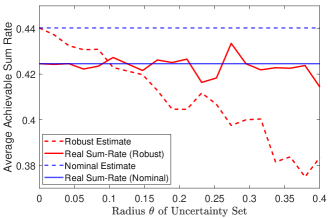
From Fig. 2, the following main points can be highlighted.

1. The nominally estimated AASR $R_{\bar{\bm{H}},\bar{\bm{X}}}$ is unreliable; recall that $\bar{\bm{X}}$ is a nominally optimal waveform adapted to $\bar{\bm{H}}$. Specifically, the true AASR $R_{\bm{H}_{0},\bar{\bm{X}}}$ is smaller than the nominally estimated AASR $R_{\bar{\bm{H}},\bar{\bm{X}}}$. This raises the issue of communication reliability: Users may experience lower data rates than the estimated ones (i.e., user dissatisfaction).

2. The robust estimate is more reliable than the nominal estimate. To be specific, the true AASR $R_{\bm{H}_{0},\bm{X}^{*}}$ can be larger than the robustly estimated AASR $R_{\bm{H}^{*},\bm{X}^{*}}$ if proper values of $\theta$ can be used in the solution method; recall $(\bm{H}^{*},\bm{X}^{*})$ in Fact 1. In this case, the best $\theta$ used in the solution method is about $0.1$. However, $\theta$ can be neither overly large nor overly small: A small $\theta$ (e.g., $\theta<0.1$) cannot provide sufficient robustness while a large $\theta$ (e.g., $\theta>0.1$) may lead to significant conservativeness. In practice, when we have no knowledge of the true channel $\bm{H}_{0}$, we can tune (e.g., trial-and-error) to find the best value of $\theta$ case by case. Also recall the discussion about the budget of uncertainty set in Subsection II-D.

3. In terms of the true AASRs evaluated at $\bar{\bm{X}}$ and $\bm{H}^{*}$, we cannot see the evident advantage of using $\bar{\bm{X}}$ over $\bm{H}^{*}$ or that of using $\bm{H}^{*}$ over $\bar{\bm{X}}$. This is theoretically easy to understand because we cannot determine which MUI energy is larger between $\|\bm{H}_{0}\bar{\bm{X}}-\bm{S}\|^{2}_{F}$ and $\|\bm{H}_{0}\bm{X}^{*}-\bm{S}\|^{2}_{F}$.

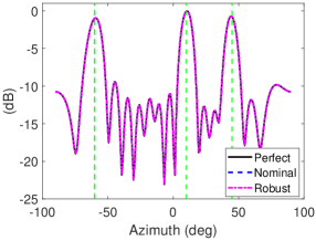
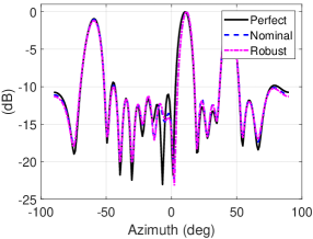
In Fig. 3, we show the beam patterns of the three waveforms: the perfect waveform $\bm{X}_{s}$ for sensing, the nominal waveform $\bar{\bm{X}}$, and the robust waveform $\bm{X}^{*}$ when $\theta=0.1$. Since this is a sensing-centric design, all waveforms are guaranteed to have the same beam pattern.

Figure 3: Beam patterns of the three waveforms are overlapped.

V-C2 Joint Robust Waveform Design (5)

We next study the case where the sensing performance is slightly sacrificed; specifically, in (5), as an example, we set $\rho=0.05$. The solution method adopted is the particle swarm optimization (PSO) algorithm; for parameter settings, see the shared source codes. The results of robust waveform design are shown in Fig. 4.

Figure 4: Resuls on joint robust waveform design. The channel capacity is $\log_{2}(1+P_{\mathsf{T}}/N_{0})=1$bps/Hz/user. The robust estimate can give a reliable lower bound of communication performance, while the nominal estimate cannot. On average, the nominal design consumes about 0.002 seconds, whereas the robust design consumes about 0.005 seconds for each $\theta$.

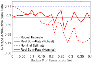
From Fig. 4, the AASRs are significantly improved when the sensing performance is slightly sacrificed; this was the original motivation for developing ISAC systems. In addition, the robust estimate can give a reliable lower bound of communication performance, while the nominal estimate cannot. In Fig. 5, we show the beam patterns of the three waveforms: $\bm{X}_{s}$, $\bar{\bm{X}}$, and $\bm{X}^{*}$ ($\theta=0.1$). Since this is not a sensing-centric design, nominally optimal and robust waveforms are not guaranteed to have the same beam pattern as the perfect waveform for sensing.

Figure 5: Beam patterns of the three waveforms are not overlapped.

VI Conclusions

This paper is concerned with the performance analysis and robust waveform design problems for ISAC systems. When there exist model uncertainties in nominal communication channels, the nominally-estimated communication performance may be unreachable. However, by considering worst-case channels and employing robust waveform design diagrams, the robustly-estimated communication performance can be guaranteed to be achievable in practice; as a result, the reliability of ISAC systems in terms of communication performance is improved. Experiments show that the robustly-estimated communication performance (i.e., average achievable sum rate; AASR) is lower than the nominally-estimated one. When an appropriate radius $\theta$ of the uncertainty set is adopted, the real AASR is guaranteed to be larger than the robustly-estimated AASR. In contrast, the nominally-estimated AASR can be larger than the true AASR, and therefore, the communication performance is not guaranteed. However, for a real-world communication problem, especially in harsh environments (e.g., large uncertainties exist in nominal models), the true radius $\theta$ of the uncertainty set may not be known, which can therefore be left as an empirically tunable parameter for specific real-world ISAC systems.

Appendix A Proof of Theorem 1

Proof:

First, we consider the max-min counterpart of (4):

$$\begin{array}[]{cl}\displaystyle\max_{\bm{H}}\min_{\bm{X}}&\|\bm{H}\bm{X}-\bm{S}\|^{2}_{F}\\ \text{s.t.}&\displaystyle\frac{1}{L}\bm{X}\bm{X}^{\mathsf{H}}=\bm{R},~{}\|\bm{H}-\bar{\bm{H}}\|\leq\theta.\end{array}$$ (21)

For every feasible $\bm{H}$, the inner sub-problem $\min_{\bm{X}:~{}\bm{X}\bm{X}^{\mathsf{H}}=L\bm{R}}\|\bm{H}\bm{X}-\bm{S}\|^{2}_{F}$ is solved by $\bm{X}^{*}_{\bm{H}}=\sqrt{L}\cdot\bm{F}\cdot\bm{U}\bm{I}_{N\times L}\bm{V}^{\mathsf{H}}$, where $\bm{U}\bm{\Sigma}\bm{V}^{\mathsf{H}}=\bm{F}^{\mathsf{H}}\bm{H}^{\mathsf{H}}\bm{S}$ means the singular value decomposition (SVD) of $\bm{F}^{\mathsf{H}}\bm{H}^{\mathsf{H}}\bm{S}$ and $\bm{I}_{N\times L}\coloneqq[\bm{I}_{N},\bm{0}_{N\times(L-N)}]$; the $N\times(L-N)$ zero matrix is denoted by $\bm{0}_{N\times(L-N)}$; see [12, Eq. (15)]. Note that the optimal solution $\bm{X}^{*}_{\bm{H}}$ depends on $\bm{H}$, and $\bm{X}^{*}_{\bm{H}}$ may not be unique given $\bm{H}$. Plugging in $\bm{X}^{*}_{\bm{H}}$ back to (21) yields (6).

Second, we show that (6) is equivalent to the original min-max problem (4). Let $\mathcal{X}\coloneqq\{\bm{X}:~{}\displaystyle\bm{X}\bm{X}^{\mathsf{H}}=L\bm{R}\}$ and $\mathcal{H}\coloneqq\{\bm{H}:~{}\|\bm{H}-\bar{\bm{H}}\|\leq\theta\}$. According to the weak min-max property, we have $\displaystyle\max_{\bm{H}\in\mathcal{H}}\min_{\bm{X}\in\mathcal{X}}\|\bm{H}\bm{X}-\bm{S}\|^{2}_{F}\leq\displaystyle\min_{\bm{X}\in\mathcal{X}}\max_{\bm{H}\in\mathcal{H}}\|\bm{H}\bm{X}-\bm{S}\|^{2}_{F}$. Therefore,

$$\begin{array}[]{l}\displaystyle\max_{\bm{H}\in\mathcal{H}}\min_{\bm{X}\in\mathcal{X}}\|\bm{H}\bm{X}-\bm{S}\|^{2}_{F}=\displaystyle\max_{\bm{H}\in\mathcal{H}}\|\bm{H}\bm{X}^{*}_{\bm{H}}-\bm{S}\|^{2}_{F}\\ \quad\quad=\displaystyle\max_{\bm{H}\in\mathcal{H}}\|\sqrt{L}\cdot\bm{H}\cdot\bm{F}\cdot\bm{U}\bm{I}_{N\times L}\bm{V}^{\mathsf{H}}-\bm{S}\|^{2}_{F}\\ \quad\quad\leq\displaystyle\min_{\bm{X}\in\mathcal{X}}\max_{\bm{H}\in\mathcal{H}}\|\bm{H}\bm{X}-\bm{S}\|^{2}_{F}.\end{array}$$

On the other hand, we have $\displaystyle\min_{\bm{X}\in\mathcal{X}}\max_{\bm{H}\in\mathcal{H}}\|\bm{H}\bm{X}-\bm{S}\|^{2}_{F}\leq\displaystyle\max_{\bm{H}\in\mathcal{H}}\|\bm{H}\bm{X}^{*}_{\bm{H}}-\bm{S}\|^{2}_{F}$, because $\bm{X}^{*}_{\bm{H}}$ is a feasible solution in $\mathcal{X}$, and the right-hand side of the above display equals to $\displaystyle\max_{\bm{H}\in\mathcal{H}}\|\sqrt{L}\cdot\bm{H}\cdot\bm{F}\cdot\bm{U}\bm{I}_{N\times L}\bm{V}^{\mathsf{H}}-\bm{S}\|^{2}_{F}$. Combining the above results, we have the strong min-max property

$$\begin{array}[]{l}\displaystyle\min_{\bm{X}\in\mathcal{X}}\max_{\bm{H}\in\mathcal{H}}\|\bm{H}\bm{X}-\bm{S}\|^{2}_{F}=\displaystyle\max_{\bm{H}\in\mathcal{H}}\min_{\bm{X}\in\mathcal{X}}\|\bm{H}\bm{X}-\bm{S}\|^{2}_{F}\\ \quad\quad\quad\quad=\displaystyle\max_{\bm{H}\in\mathcal{H}}\|\sqrt{L}\cdot\bm{H}\cdot\bm{F}\cdot\bm{U}\bm{I}_{N\times L}\bm{V}^{\mathsf{H}}-\bm{S}\|^{2}_{F}.\end{array}$$

Suppose that $\bm{H}^{*}$ solves the maximization problem in the second line of the above display; $\bm{H}^{*}$ may not be unique. Then $(\bm{X}^{*}_{\bm{H}^{*}},~{}\bm{H}^{*})$ forms a saddle point, completing the proof. $\square$∎

Appendix B Proof of Proposition 1

The boundedness of $f$ is natural. Below we focus on the Lipschitz continuity of $f$. One may verify that it is difficult to prove the continuity of $f$ directly using the definition in (7) because the SVD of a matrix might not be unique; specifically, given $\bm{H}$, there may exist multiple $\bm{U}$s and $\bm{V}$s such that $\bm{U}\bm{\Sigma}\bm{V}^{\mathsf{H}}=\bm{F}^{\mathsf{H}}\bm{H}^{\mathsf{H}}\bm{S}$. The complication arises when $\bm{U}$ and $\bm{V}$ correspond to zero singular value(s) in $\bm{\Sigma}$. We, therefore, investigate the continuity of $f$ from its original definition. In addition, the existence of $B$ is guaranteed due to the equivalence of norms on a finite-dimensional linear space.

Proof:

Recall that $f(\bm{H})\coloneqq\min_{\bm{X}\in\mathcal{X}}\|\bm{H}\bm{X}-\bm{S}\|^{2}_{F}$ where $\mathcal{X}\coloneqq\{\bm{X}:~{}\bm{X}\bm{X}^{\mathsf{H}}=L\bm{R}\}$. First, note that for every $\bm{X}\in\mathcal{X}$ and every $\bm{H}_{1},\bm{H}_{2}\in\mathcal{H}$, there exists an upper bound $0<B_{1}<\infty$ such that $\|\bm{H}_{1}\bm{X}-\bm{S}\|_{F}+\|\bm{H}_{2}\bm{X}-\bm{S}\|_{F}\leq B_{1}$. A loose choice can be $B_{1}\coloneqq 2\sqrt{LP_{\mathsf{T}}}\cdot(\|\bar{\bm{H}}\|_{F}+B\theta)+2\|\bm{S}\|_{F}$ where $0<B<\infty$ is a real-valued constant such that $\|\bm{H}_{1}-\bar{\bm{H}}\|_{F}\leq B\|\bm{H}_{1}-\bar{\bm{H}}\|$; the existence of $B$ is guaranteed due to the equivalence of norms on a finite-dimensional linear space. Just note that $|\|\bm{H}_{1}\|_{F}-\|\bar{\bm{H}}\|_{F}|\leq\|\bm{H}_{1}-\bar{\bm{H}}\|_{F}\leq B\|\bm{H}_{1}-\bar{\bm{H}}\|\leq B\theta$. The same argument also holds for $\bm{H}_{2}$. Hence, for every $\bm{H}_{1},\bm{H}_{2}\in\mathcal{H}$, we have

$$\begin{array}[]{l}|f(\bm{H}_{1})-f(\bm{H}_{2})|\\ \quad\quad=\Big{|}\displaystyle\min_{\bm{X}\in\mathcal{X}}\|\bm{H}_{1}\bm{X}-\bm{S}\|^{2}_{F}-\displaystyle\min_{\bm{X}\in\mathcal{X}}\|\bm{H}_{2}\bm{X}-\bm{S}\|^{2}_{F}\Big{|}\\ \quad\quad\leq\displaystyle\max_{\bm{X}\in\mathcal{X}}\Big{|}\|\bm{H}_{1}\bm{X}-\bm{S}\|^{2}_{F}-\|\bm{H}_{2}\bm{X}-\bm{S}\|^{2}_{F}\Big{|}\\ \quad\quad=\displaystyle\max_{\bm{X}\in\mathcal{X}}\Big{|}\Big{(}\|\bm{H}_{1}\bm{X}-\bm{S}\|_{F}+\|\bm{H}_{2}\bm{X}-\bm{S}\|_{F}\Big{)}\cdot\\ \quad\quad\quad\quad\quad\quad\Big{(}\|\bm{H}_{1}\bm{X}-\bm{S}\|_{F}-\|\bm{H}_{2}\bm{X}-\bm{S}\|_{F}\Big{)}\Big{|}\\ \quad\quad\leq\displaystyle\max_{\bm{X}\in\mathcal{X}}\Big{|}\|\bm{H}_{1}\bm{X}-\bm{S}\|_{F}+\|\bm{H}_{2}\bm{X}-\bm{S}\|_{F}\Big{|}\cdot\\ \quad\quad\quad\quad\quad\quad\Big{|}\|\bm{H}_{1}\bm{X}-\bm{S}\|_{F}-\|\bm{H}_{2}\bm{X}-\bm{S}\|_{F}\Big{|}\\ \quad\quad\leq B_{1}\cdot\displaystyle\max_{\bm{X}\in\mathcal{X}}\Big{\|}\bm{H}_{1}\bm{X}-\bm{H}_{2}\bm{X}\Big{\|}_{F}\\ \quad\quad\leq B_{1}\cdot\Big{\|}\bm{H}_{1}-\bm{H}_{2}\Big{\|}_{F}\cdot\displaystyle\max_{\bm{X}\in\mathcal{X}}\Big{\|}\bm{X}\Big{\|}_{F}\\ \quad\quad=B_{1}\sqrt{LP_{\mathsf{T}}}\cdot\|\bm{H}_{1}-\bm{H}_{2}\|_{F}\\ \quad\quad\leq B_{1}\sqrt{LP_{\mathsf{T}}}\cdot B\|\bm{H}_{1}-\bm{H}_{2}\|.\end{array}$$

Note that $\|\bm{X}\|_{F}=\sqrt{\operatorname{Tr}\bm{X}^{\mathsf{H}}\bm{X}}=\sqrt{L\cdot\operatorname{Tr}\bm{R}}=\sqrt{LP_{\mathsf{T}}}$. $\square$∎

Appendix C Proof of Proposition 2

Proof:

First, from (7), $f(\bm{H})=\min_{\bm{X}:~{}\bm{X}\bm{X}^{\mathsf{H}}=L\bm{R}}\|\bm{H}\bm{X}-\bm{S}\|^{2}_{F}=\operatorname{Tr}[L\bm{H}^{\mathsf{H}}\bm{H}\bm{R}]+\operatorname{Tr}[\bm{S}^{\mathsf{H}}\bm{S}]-2\operatorname{Tr}[\sqrt{L}\bm{S}^{\mathsf{H}}\bm{H}\bm{F}\cdot\bm{U}\bm{I}_{N\times L}\bm{V}^{\mathsf{H}}]$, where $\bm{U}\bm{\Sigma}\bm{V}^{\mathsf{H}}=\bm{F}^{\mathsf{H}}\bm{H}^{\mathsf{H}}\bm{S}$ denotes the SVD of $\bm{F}^{\mathsf{H}}\bm{H}^{\mathsf{H}}\bm{S}$. Since $\operatorname{rank}(\bm{F}^{\mathsf{H}}\bm{H}^{\mathsf{H}}\bm{S})\leq\min\{\operatorname{rank}(\bm{F}),\operatorname{rank}(\bm{H}),\operatorname{rank}(\bm{S})\}\leq K=\min\{K,N,L\}$, the singular value matrix $\bm{\Sigma}\in\mathbb{C}^{N\times L}$ has zero singular value(s), and therefore, $\bm{U}$ and $\bm{V}$ are even not unique. As a result, the derivative of $f$ with respect to $\bm{H}$, i.e.,

$$\frac{\mathrm{d}f(\bm{H})}{\mathrm{d}\bm{H}}=L\bm{H}\bm{R}+L\bm{H}\bm{R}^{\mathsf{H}}-2\sqrt{L}\frac{\mathrm{d}\operatorname{Tr}[\bm{S}^{\mathsf{H}}\bm{H}\bm{F}\cdot\bm{U}\bm{I}_{N\times L}\bm{V}^{\mathsf{H}}]}{\mathrm{d}\bm{H}},$$

is not well-defined. Recall that $\bm{U}$ and $\bm{V}$ depend on $\bm{H}$.

The non-convexity and non-concavity of the objective function $f(\bm{H})=\min_{\bm{X}:~{}\bm{X}\bm{X}^{\mathsf{H}}=L\bm{R}}\|\bm{H}\bm{X}-\bm{S}\|^{2}_{F}$ can be verified through the definitions of convexity and concavity by constructing counterexamples, which completes the proof. $\square$∎

Appendix D Proof of Proposition 3

Proof:

The upper bound is obtained by plugging $\bar{\bm{X}}$ into the optimization problem $f(\bm{H})\coloneqq\min_{\bm{X}:~{}\bm{X}\bm{X}^{\mathsf{H}}=L\bm{R}}\|\bm{H}\bm{X}-\bm{S}\|^{2}_{F}$ because $\bar{\bm{X}}$ is a feasible solution. The lower bound is obtained by the reverse triangle inequality, i.e., $\|\bm{H}\bm{X}-\bm{S}\|_{F}\geq|\|\bm{H}\bm{X}\|_{F}-\|\bm{S}\|_{F}|$; note that $\|\bm{H}\bm{X}\|_{F}=\sqrt{L\operatorname{Tr}[\bm{H}^{\mathsf{H}}\bm{H}\bm{R}]}$ because $\bm{X}\bm{X}^{\mathsf{H}}=L\bm{R}$. The upper bound is positive-definite quadratic (thus convex) in $\operatorname{vec}(\bm{H})$ because $\bar{\bm{X}}\bar{\bm{X}}^{\mathsf{H}}=L\bm{R}$ and $\bm{R}$ is positive definite. Since at the center $\bar{\bm{H}}$ of $\mathcal{H}$ we have $f(\bar{\bm{H}})=\overline{f}(\bar{\bm{H}})$, the upper bound is tight. Also, the reverse triangle inequality is tight, and therefore, the lower bound is tight. The third claim is obvious. We show the uniform bound in the fourth claim below. We have

$$\begin{array}[]{cl}\bar{f}(\bm{H})-f(\bm{H})&=\bar{f}(\bm{H})-\bar{f}(\bar{\bm{H}})+f(\bar{\bm{H}})-f(\bm{H})\\ &\leq|\bar{f}(\bm{H})-\bar{f}(\bar{\bm{H}})|+|f(\bar{\bm{H}})-f(\bm{H})|\\ &\leq L_{f}\|\bm{H}-\bar{\bm{H}}\|+L_{f}\|\bm{H}-\bar{\bm{H}}\|\\ &\leq 2L_{f}\cdot\theta.\end{array}$$

This completes the proof. $\square$∎

Appendix E Proof of Proposition 4

Proof:

The Hessian of the objective function in terms of $\operatorname{vec}(\bm{H})$ is

$$\begin{array}[]{l}L((\bm{F}\bm{A})^{\mathsf{T}}\otimes\bm{I}_{K})^{\mathsf{H}}((\bm{F}\bm{A})^{\mathsf{T}}\otimes\bm{I}_{K})\\ \quad\quad\quad=L\{[(\bm{F}\bm{A})^{\mathsf{T}}]^{\mathsf{H}}\otimes\bm{I}^{\mathsf{H}}_{K}\}\{(\bm{F}\bm{A})^{\mathsf{T}}\otimes\bm{I}_{K}\}\\ \quad\quad\quad=L[(\bm{F}\bm{A})^{\mathsf{T}}]^{\mathsf{H}}(\bm{F}\bm{A})^{\mathsf{T}}\otimes\bm{I}^{\mathsf{H}}_{K}\bm{I}_{K}\\ \quad\quad\quad=L[(\bm{F}\bm{A})(\bm{F}\bm{A})^{\mathsf{H}}]^{\mathsf{T}}\otimes\bm{I}^{\mathsf{H}}_{K}\bm{I}_{K}\\ \quad\quad\quad=L\bm{R}^{\mathsf{T}}\otimes\bm{I}_{K}\succ\bm{0},\end{array}$$

because the beampattern-inducing matrix $\bm{R}$ is positive definite. Hence, the objective function of (11) is positive definite in $\operatorname{vec}(\bm{H})$, and therefore, convex in $\operatorname{vec}(\bm{H})$. The convexity of the objective function in terms of $\operatorname{vec}(\bm{A})$ can be shown in a similar way: just note that the objective function can only be shown to be positive semi-definite because the Hessian $L(\bm{I}_{L}\otimes\bm{H}\bm{F})^{\mathsf{H}}(\bm{I}_{L}\otimes\bm{H}\bm{F})$ is not necessarily positive definite.

The feasible region of $\bm{H}$ is convex because the norm constraint is convex and the equality constraint is linear. The feasible region of $\bm{A}$ is convex because it is built by a linear equality constraint. This completes the proof. $\square$∎

Appendix F Proof of Corollary 1

Proof:

According to Proposition 4, we immediately have $\bm{C}^{\mathsf{T}}\bm{C}\succ\bm{0}$, and therefore, $p(\bm{h})$ is positive definite in $\bm{h}$. In addition, we have $p(\bm{h})-\frac{\mu}{2}\bm{h}^{\mathsf{T}}\bm{h}=\bm{h}^{\mathsf{T}}(\bm{C}^{\mathsf{T}}\bm{C}-\frac{\mu}{2}\bm{I}_{2KN})\bm{h}-2\bm{s}^{\mathsf{T}}\bm{C}\bm{h}+\bm{s}^{\mathsf{T}}\bm{s}$, where $\mu>0$ is a positive number. Since $\bm{C}^{\mathsf{T}}\bm{C}\succ\bm{0}$, there exist $\mu>0$ such that $\bm{C}^{\mathsf{T}}\bm{C}-\frac{\mu}{2}\bm{I}_{2KN}\succeq\bm{0}$. As a result, the function $p(\bm{h})-\frac{\mu}{2}\bm{h}^{\mathsf{T}}\bm{h}$ can be a convex function for some $\mu>0$, which means that the objective function $p(\bm{h})$ of (14) is strongly convex. $\square$∎

Appendix G Proof of Proposition 5

Proof:

According to [43, Thm. 1], a point $\bm{y}$ is a globally optimal solution to (14) if and only if $\left<{\nabla p(\bm{y})},{~{}\bm{h}-\bm{y}}\right>\leq 0$, for every $\bm{h}$ such that $\|\bm{h}-\bar{\bm{h}}\|\leq\theta$, where $\nabla p(\bm{y})$ denotes the gradient of $p$ evaluated at $\bm{y}$. Therefore, if we have $\max_{\bm{y}\in\mathcal{Y}}\max_{\bm{h}:\|\bm{h}-\bar{\bm{h}}\|\leq\theta}\left<{\nabla p(\bm{y})},{~{}\bm{h}-\bm{y}}\right>\leq 0$, for some dedicated $\mathcal{Y}$, then every $\bm{y}$ that solves the above optimization is a global maximum of (14). This proposition, which is adapted from [43, Algo. 1] for the problem (14), formalizes the above intuition. The global optimality and convergence are therefore guaranteed by [43, Thm. 4]. For rigorous and complete technical proof, see [43]; just note that in (15), the equality constraint can be changed to its convex inequality counterpart because the optima of linear objective functions lie on the boundary of feasible regions. $\square$∎

Appendix H Proof of Proposition 6

Proof:

Problem (16) is equivalent to

$$\begin{array}[]{cl}\displaystyle\max_{\bm{z}\in\mathbb{R}^{2KN}}&(\bm{y}^{\mathsf{T}}_{k}\bm{C}^{\mathsf{T}}\bm{C}-\bm{s}^{\mathsf{T}}\bm{C})\cdot(\theta\bm{z}+\bar{\bm{h}}),~{}\text{s.t.}~{}\|\bm{z}\|_{2}=1.\end{array}$$ (22)

Due to Cauchy–Schwarz inequality, the maximum is

$$\bm{z}^{*}=\frac{\bm{C}^{\mathsf{T}}\bm{C}\bm{y}_{k}-\bm{C}^{\mathsf{T}}\bm{s}}{\|\bm{C}^{\mathsf{T}}\bm{C}\bm{y}_{k}-\bm{C}^{\mathsf{T}}\bm{s}\|_{2}}.$$

As a result, a maximum of (16) is $\bm{h}^{*}=\theta\bm{z}^{*}+\bar{\bm{h}}$. $\square$∎

Appendix I Proof of Theorem 2

Proof:

In terms of $\bm{U}$, we can rewrite (13) as

$$\begin{array}[]{cl}\displaystyle\min_{\bm{U}}\|\bm{U}\bm{A}_{1}-\bm{B}_{1}\|^{2}_{F},~{}~{}\text{s.t.}~{}~{}\bm{U}\bm{U}^{\mathsf{H}}=\bm{I}_{N},\end{array}$$ (23)

where $\bm{A}_{1}$ and $\bm{B}_{1}$ are defined in Theorem 2. Problem (23) is a standard orthogonal Procrustes problem whose closed-form solution is given in Theorem 2; see technical details in [44].

In terms of $\bm{V}$, we can rewrite (13) as

$$\begin{array}[]{cl}\displaystyle\min_{\bm{V}}\|\bm{V}\bm{A}_{2}-\bm{B}_{2}\|^{2}_{F},~{}~{}\text{s.t.}~{}~{}\bm{V}\bm{V}^{\mathsf{H}}=\bm{I}_{L},\end{array}$$ (24)

where $\bm{A}_{2}$ and $\bm{B}_{2}$ are defined in Theorem 2. Problem (24) is a standard orthogonal Procrustes problem whose closed-form solution is given in Theorem 2; see technical details in [44].

In terms of $\bm{\Sigma}$, Problem (13) is a positive-definite-quadratic convex program. Note that the space $\Omega_{N\times L}$ of the matrices with diagonal, non-negative, and real entries is convex. Therefore, the projected gradient descent produces the optimal solution. The gradient of the objective function of (13) with respect to $\bm{\Sigma}$ is $2\bm{U}^{\mathsf{H}}(\bm{U}\bm{\Sigma}\bm{V}^{\mathsf{H}}-\bm{F}^{\mathsf{H}}\bm{H}^{*\mathsf{H}}\bm{S})\bm{V}=2\bm{\Sigma}-2\bm{U}^{\mathsf{H}}\bm{F}^{\mathsf{H}}\bm{H}^{*\mathsf{H}}\bm{S}\bm{V}$. Therefore, the optimal solution is given by the projected point of $\bm{U}^{\mathsf{H}}\bm{F}^{\mathsf{H}}\bm{H}^{*\mathsf{H}}\bm{S}\bm{V}$ onto $\Omega_{N\times L}$. $\square$∎

Appendix J Proof of Proposition 7

Proof:

Let $\mathcal{X}\coloneqq\{\bm{X}:~{}\|\bm{X}\|^{2}_{F}=LP_{\mathsf{T}}\}$. For every $\bm{H}_{1},\bm{H}_{2}\in\mathcal{H}$, we have

$$\begin{array}[]{l}|g(\bm{H}_{1})-g(\bm{H}_{2})|\\ \quad\quad=\Big{|}\displaystyle\min_{\bm{X}\in\mathcal{X}}\rho\|\bm{H}_{1}\bm{X}-\bm{S}\|^{2}_{F}+(1-\rho)\|\bm{X}-\bm{X}_{s}\|^{2}_{F}-\\ \quad\quad\quad\quad\displaystyle\min_{\bm{X}\in\mathcal{X}}\rho\|\bm{H}_{2}\bm{X}-\bm{S}\|^{2}_{F}+(1-\rho)\|\bm{X}-\bm{X}_{s}\|^{2}_{F}\Big{|}\\ \quad\quad\leq\displaystyle\max_{\bm{X}\in\mathcal{X}}\Big{|}\big{[}\rho\|\bm{H}_{1}\bm{X}-\bm{S}\|^{2}_{F}+(1-\rho)\|\bm{X}-\bm{X}_{s}\|^{2}_{F}\big{]}-\\ \quad\quad\quad\quad\big{[}\rho\|\bm{H}_{2}\bm{X}-\bm{S}\|^{2}_{F}+(1-\rho)\|\bm{X}-\bm{X}_{s}\|^{2}_{F}\big{]}\Big{|}\\ \quad\quad=\rho\cdot\displaystyle\max_{\bm{X}\in\mathcal{X}}\Big{|}\|\bm{H}_{1}\bm{X}-\bm{S}\|^{2}_{F}-\|\bm{H}_{2}\bm{X}-\bm{S}\|^{2}_{F}\Big{|}\\ \quad\quad\leq\rho\cdot L_{f}\cdot\|\bm{H}_{1}-\bm{H}_{2}\|.\end{array}$$

This completes the proof. $\square$∎

Appendix K Details on Experiments

In this appendix, we detail the logic flow upon which the shared source codes are written.

Algorithm 1 Simulation Engine

Definition: Let $I$ denote the number of Monte–Carlo episodes.

Remark: The notation $0:0.02:0.4$ means a discrete vector starting at $0$, ending with $0.4$, and uniformly spaced with $0.02$.

1:$I=25$

2:// Stage 1: Engine Initialization

3:$N\leftarrow 16$, $K\leftarrow 4$, $L\leftarrow 30$, $f\leftarrow 6\times 10^{9}$, $P_{\mathsf{T}}\leftarrow 1$, $\theta\leftarrow 0:0.02:0.4$

4:Generate $\bm{H}_{\text{ref}}$

5:Design Ideal Sensing Waveform $\bm{X}_{s}$

6:// Stage 2: Offline Design Using Practically Available Nominal Channel

7:Generate Constellation $\bm{S}$

8:Generate Nominal Channel $\bar{\bm{H}}$ From $\{\bm{H}:\|\bm{H}-\bm{H}_{\text{ref}}\|_{\max}\leq 0.4\}$

9:Design Nominally Optimal Waveform $\bar{\bm{X}}$ Using $\bar{\bm{H}}$

10:Calculate Nominally Estimated AASR $R_{\bar{\bm{H}},\bar{\bm{X}}}$

11:Design Robust Waveform $\bm{X}^{*}$ Using $\bar{\bm{H}}$ for Every $\theta$ (NB: $\bm{X}^{*}$ depends on $\theta$)

12:Calculate Robustly Estimated AASR $R_{\bm{H}^{*},\bm{X}^{*}}$

13:// Stage 3: Online Test Using Random And Practically Unknown True Channel

14:$i\leftarrow 0$

15:while true do

16:     // Calculate True AASRs

17:     Uniformly Generate $\bm{H}_{0}$ From $\{\bm{H}:\|\bm{H}-\bm{H}_{\text{ref}}\|_{\max}\leq 0.4\}$

18:     Calculate True AASR $R_{\bm{H}_{0},\bar{\bm{X}}}$ at Nominally Optimal Waveform $\bar{\bm{X}}$

19:     Calculate True AASR $R_{\bm{H}_{0},\bm{X}^{*}}$ at Robust Waveform $\bm{X}^{*}$ for Every $\theta$ (NB: $\bm{X}^{*}$ depends on $\theta$)

20:     // Next Episode

21:     $i\leftarrow i+1$

22:     // End of Simulation

23:     if $i>I$ then

24:         break while

25:     end if

26:end while

27:AASRs averaged over $I$ episodes

Dr. Shixiong Wang (Member, IEEE) received the B.Eng. degree in detection, guidance, and control technology, and the M.Eng. degree in systems and control engineering from the School of Electronics and Information, Northwestern Polytechnical University, China, in 2016 and 2018, respectively. He received his Ph.D. degree from the Department of Industrial Systems Engineering and Management, National University of Singapore, Singapore, in 2022. He is currently a Postdoctoral Research Associate with the Intelligent Transmission and Processing Laboratory, Imperial College London, London, United Kingdom, from May 2023. He was a Postdoctoral Research Fellow with the Institute of Data Science, National University of Singapore, Singapore, from March 2022 to March 2023. His research interest includes statistics and optimization theories with applications in signal processing, machine learning, and control technology.

Dr. Wei Dai (Member, IEEE) received the Ph.D. degree from the University of Colorado Boulder, Boulder, Colorado, in 2007. He is currently a Senior Lecturer (Associate Professor) in the Department of Electrical and Electronic Engineering, Imperial College London, London, UK. From 2007 to 2011, he was a Postdoctoral Research Associate with the University of Illinois Urbana-Champaign, Champaign, IL, USA. He was an Associate Editor for IEEE Transactions on Signal Processing (2020). The main theme of his interdisciplinary research interests is sparse signal processing, including compressed sensing, super-resolution, and bilinear problems. His research interests include electromagnetic sensing, biomedical imaging, wireless communications, and information theory.

Dr. Haowei Wang is currently a research scientist at Rice-Rick Digitalization PTE. Ltd. Before joining Rice-Rick, he received the B.Eng. degree in industrial engineering from Nanjing University in 2016 and the Ph.D. degree in industrial and systems engineering from National University of Singapore(NUS) in 2021. His research interest includes simulation optimization, Bayesian optimization under uncertainties.

Dr. Geoffrey Ye Li (Fellow, IEEE) is currently a Chair Professor with Imperial College London, U.K. Before joining Imperial in 2020, he was a Professor with the Georgia Institute of Technology, USA, for 20 years and a Principal Technical Staff Member with AT&T Labs-Research, New Jersey, USA, for five years. His general research interests include statistical signal processing and machine learning for wireless communications. Dr. Li was awarded an IEEE Fellow and an IET Fellow for his contributions to signal processing for wireless communications. He won several prestigious awards from IEEE Signal Processing, Vehicular Technology, and Communications Societies, including IEEE ComSoc Edwin Howard Armstrong Achievement Award in 2019. He also received the 2015 Distinguished ECE Faculty Achievement Award from Georgia Tech. He has been involved in editorial activities for over 20 technical journals, including the founding Editor-in-Chief of IEEE Journal on Selected Areas in Communications Special Series on ML in Communications and Networking. He has organized and chaired many international conferences, including the Technical Program Vice-Chair of the IEEE ICC’03, and the General Co-Chair of the IEEE GlobalSIP’14, the IEEE VTC’19 Fall, the IEEE SPAWC’20, and the IEEE VTC’22 Fall.

References

- [1] F. Liu, C. Masouros, A. P. Petropulu, H. Griffiths, and L. Hanzo, “Joint radar and communication design: Applications, state-of-the-art, and the road ahead,” IEEE Trans. on Commun., vol. 68, no. 6, pp. 3834–3862, 2020.
- [2] J. A. Zhang, F. Liu, C. Masouros, R. W. Heath, Z. Feng, L. Zheng, and A. Petropulu, “An overview of signal processing techniques for joint communication and radar sensing,” IEEE Journal of Selected Topics in Signal Processing, vol. 15, no. 6, pp. 1295–1315, 2021.
- [3] A. Liu, Z. Huang, M. Li, Y. Wan, W. Li, T. X. Han, C. Liu, R. Du, D. K. P. Tan, J. Lu et al., “A survey on fundamental limits of integrated sensing and communication,” IEEE Commun. Surveys & Tutorials, vol. 24, no. 2, pp. 994–1034, 2022.
- [4] W. Zhou, R. Zhang, G. Chen, and W. Wu, “Integrated sensing and communication waveform design: A survey,” IEEE Open Journal of the Communications Society, vol. 3, pp. 1930–1949, 2022.
- [5] Y. Xiong, F. Liu, Y. Cui, W. Yuan, T. X. Han, and G. Caire, “On the fundamental tradeoff of integrated sensing and communications under gaussian channels,” IEEE Trans. on Inform. Theory, 2023.
- [6] B. Tang, J. Tang, and Y. Peng, “Mimo radar waveform design in colored noise based on information theory,” IEEE Trans. on Signal Processing, vol. 58, no. 9, pp. 4684–4697, 2010.
- [7] X. Yuan, Z. Feng, J. A. Zhang, W. Ni, R. P. Liu, Z. Wei, and C. Xu, “Spatio-temporal power optimization for mimo joint communication and radio sensing systems with training overhead,” IEEE Trans. on Veh. Technol., vol. 70, no. 1, pp. 514–528, 2020.
- [8] P. Kumari, S. A. Vorobyov, and R. W. Heath, “Adaptive virtual waveform design for millimeter-wave joint communication–radar,” IEEE Trans. on Signal Processing, vol. 68, pp. 715–730, 2019.
- [9] T. M. Cover and J. A. Thomas, Elements of Information Theory, 2nd ed. John Wiley & Sons, 2006.
- [10] B. Guo, J. Liang, G. Wang, B. Tang, and H. So, “Bistatic mimo dfrc system waveform design via fractional programming,” IEEE Trans. on Signal Processing, 2023.
- [11] Z. Wei, J. Piao, X. Yuan, H. Wu, J. A. Zhang, Z. Feng, L. Wang, and P. Zhang, “Waveform design for mimo-ofdm integrated sensing and communication system: An information theoretical approach,” IEEE Trans. on Commun., 2023.
- [12] F. Liu, L. Zhou, C. Masouros, A. Li, W. Luo, and A. Petropulu, “Toward dual-functional radar-communication systems: Optimal waveform design,” IEEE Trans. on Signal Processing, vol. 66, no. 16, pp. 4264–4279, 2018.
- [13] X. Li, V. C. Andrei, U. J. Mönich, and H. Boche, “Optimal and robust waveform design for mimo-ofdm channel sensing: A cramer-rao bound perspective,” in 2023 IEEE International Conference on Communications, 2023.
- [14] A. Mukherjee and A. L. Swindlehurst, “Robust beamforming for security in mimo wiretap channels with imperfect csi,” IEEE Trans. on Signal Processing, vol. 59, no. 1, pp. 351–361, 2010.
- [15] F. Liu, C. Masouros, A. Li, and T. Ratnarajah, “Robust mimo beamforming for cellular and radar coexistence,” IEEE Wireless Commun. Letters, vol. 6, no. 3, pp. 374–377, 2017.
- [16] N. Zhao, Y. Wang, Z. Zhang, Q. Chang, and Y. Shen, “Joint transmit and receive beamforming design for integrated sensing and communication,” IEEE Commun. Letters, vol. 26, no. 3, pp. 662–666, 2022.
- [17] Z. Ren, L. Qiu, J. Xu, and D. W. K. Ng, “Robust transmit beamforming for secure integrated sensing and communication,” IEEE Trans. on Commun., 2023.
- [18] M. Luan, B. Wang, Z. Chang, T. Hämäläinen, and F. Hu, “Robust beamforming design for ris-aided integrated sensing and communication system,” IEEE Trans. on Intell. Transport. Syst., 2023.
- [19] D. R. Fuhrmann and G. San Antonio, “Transmit beamforming for mimo radar systems using signal cross-correlation,” IEEE Trans. on Aerosp. Electron. Syst., vol. 44, no. 1, pp. 171–186, 2008.
- [20] S. Ahmed and I. M. Jaimoukha, “A relaxation-based approach for the orthogonal procrustes problem with data uncertainties,” in Proceedings of 2012 UKACC International Conference on Control. IEEE, 2012, pp. 906–911.
- [21] Y. Liu, Z. Tan, H. Hu, L. J. Cimini, and G. Y. Li, “Channel estimation for ofdm,” IEEE Commun. Surveys & Tutorials, vol. 16, no. 4, pp. 1891–1908, 2014.
- [22] D. Neumann, T. Wiese, and W. Utschick, “Learning the mmse channel estimator,” IEEE Trans. on Signal Processing, vol. 66, no. 11, pp. 2905–2917, 2018.
- [23] M. Soltani, V. Pourahmadi, A. Mirzaei, and H. Sheikhzadeh, “Deep learning-based channel estimation,” IEEE Commun. Letters, vol. 23, no. 4, pp. 652–655, 2019.
- [24] Y. D. Sergeyev, R. G. Strongin, and D. Lera, Introduction to global optimization exploiting space-filling curves. Springer Science & Business Media, 2013.
- [25] D. Tse and P. Viswanath, Fundamentals of Wireless Communication. Cambridge University Press, 2005.
- [26] S. Desale, A. Rasool, S. Andhale, and P. Rane, “Heuristic and meta-heuristic algorithms and their relevance to the real world: a survey,” International Journal of Computer Engineering in Research Trends, vol. 351, no. 5, pp. 2349–7084, 2015.
- [27] R. Mart, P. M. Pardalos, and M. G. Resende, Handbook of Heuristics. Springer Publishing, 2018.
- [28] A. Kaveh and T. Bakhshpoori, Metaheuristics: Outlines, MATLAB Codes, and Examples. Springer, 2019.
- [29] E. D. Taillard, Design of Heuristic Algorithms for Hard Optimization. Springer Publishing, 2023.
- [30] E. Vazquez and J. Bect, “Convergence properties of the expected improvement algorithm with fixed mean and covariance functions,” Journal of Statistical Planning and Inference, vol. 140, no. 11, pp. 3088–3095, 2010.
- [31] A. D. Bull, “Convergence rates of efficient global optimization algorithms.” Journal of Machine Learning Research, vol. 12, no. 10, 2011.
- [32] B. Shahriari, K. Swersky, Z. Wang, R. P. Adams, and N. De Freitas, “Taking the human out of the loop: A review of Bayesian optimization,” Proceedings of the IEEE, vol. 104, no. 1, pp. 148–175, 2015.
- [33] D. R. Jones, M. Schonlau, and W. J. Welch, “Efficient global optimization of expensive black-box functions,” Journal of Global optimization, vol. 13, pp. 455–492, 1998.
- [34] E. Björnson, L. Sanguinetti, H. Wymeersch, J. Hoydis, and T. L. Marzetta, “Massive mimo is a reality—what is next?: Five promising research directions for antenna arrays,” Digital Signal Processing, vol. 94, pp. 3–20, 2019.
- [35] D. Eriksson, M. Pearce, J. Gardner, R. D. Turner, and M. Poloczek, “Scalable global optimization via local bayesian optimization,” Advances in Neural Information Processing Systems, vol. 32, 2019.
- [36] C. Malherbe and N. Vayatis, “Global optimization of lipschitz functions,” in International Conference on Machine Learning. PMLR, 2017, pp. 2314–2323.
- [37] A. Ben-Tal and E. Roos, “An algorithm for maximizing a convex function based on its minimum,” INFORMS Journal on Computing, vol. 34, no. 6, pp. 3200–3214, 2022.
- [38] H.-K. Xu, “Averaged mappings and the gradient-projection algorithm,” Journal of Optimization Theory and Applications, vol. 150, pp. 360–378, 2011.
- [39] M. Clerc, Particle Swarm Optimization. John Wiley & Sons, 2010, vol. 93.
- [40] P. J. Van Laarhoven, E. H. Aarts, P. J. van Laarhoven, and E. H. Aarts, Simulated Annealing. Springer, 1987.
- [41] M. Dorigo and T. Stützle, Ant Colony Optimization: Overview and Recent Advances. Springer, 2019.
- [42] P. Stoica, J. Li, and X. Zhu, “Waveform synthesis for diversity-based transmit beampattern design,” IEEE Trans. on Signal Processing, vol. 56, no. 6, pp. 2593–2598, 2008.
- [43] R. Enhbat, “An algorithm for maximizing a convex function over a simple set,” Journal of Global Optimization, vol. 8, pp. 379–391, 1996.
- [44] R. Everson, “Orthogonal, but not orthonormal, procrustes problems,” Advances in Computational Mathematics, vol. 3, no. 4, 1998.
![[Uncaptioned image]](/html/2311.00071/assets/x6.png) |