Escape from a potential well under forcing and dissipation with applications to ship capsize

Abstract

Escape from a potential well occurs in a wide variety of physical systems from chemical reactions to ship capsize. In these situations escape often occurs by passage over a normally hyperbolic submanifold (NHS). This paper describes the computational implementation of an algorithm to identify the NHS of a two degree of freedom model for ship motion under the influence of damping and aperiodic forcing. Additionally we demonstrate how the stable manifolds of these submanifolds can be used to classify initial ship states as safe or unsafe.

1 Introduction

Escape from a potential well is a phenomenon with widespread relevance, such as ionization of a hydrogen atom under an electromagnetic field in atomic physics jaffe1999transition , transport of defects in solid-state and semiconductor physics eckhardt1995transition , isomerization of clusters komatsuzaki2001dynamical , reaction rates in chemical physics eyring1935activated ; wigner1938transition ; wiggins2001impenetrable , buckling modes in structural mechanics collins2012isomerization ; zhong2018tube , ship motion and capsize virgin1989approx ; thompson1996suppression ; naik2017geometry , escape and recapture of comets and asteroids in celestial mechanics jaffe2002statistical ; dellnitz2005transport , and escape into inflation or recollapse to singularity in cosmology deoliveira2002homoclinic .

Although the autonomous Hamiltonian case and its extension to periodic forcing and damping are well-studied, developing the theory to allow aperiodic forcing is important for many real-world applications. There is substantial work on stochastic forcing, but the emphasis there is on probabilistic results with respect to the distribution of the forcing, whereas we want results for specified realisations of the forcing. Even though the perturbation methods developed in nayfeh1973nonlinear are useful for deriving algebraic conditions for dynamical behaviours, a geometric viewpoint highlights the dynamical (phase space) mechanism of capsize. This viewpoint was developed in studies by thompson1996suppression ; falzarano1992application using the paradigm of the escape from a potential well for capsize and lobe dynamics as the mechanism of eroding the non-capsize region in the well. This viewpoint was further developed to include stochastic forcing in naik2017geometry and dissipative, gyroscopic forcing in zhong2020geometry . The viewpoint of the dynamical systems mechanism of crossing a saddle in the presence of dissipation and forcing has been studied extensively in the context of chemical reactions to compute reaction rates accurately based on the dividing manifold hernandez2010transition ; pollak2005reaction ; craven2017lagrangian .

The paper bishnani2003safety proposed a mathematical approach to quantifying escape from a potential well for systems with aperiodic time-dependent forcing and damping in the particular context of ship capsize. Here, we report on the computational aspects of the approach.

As is standard for a non-autonomous system on a manifold $\mathbb{M}$, we consider the flow on the extended state space $\mathbb{M}\times\mathbb{R}$. A key role in the theory of bishnani2003safety is played by a normally hyperbolic submanifold (NHS) for the dynamics in the extended state space. It is a (locally) invariant set that hovers on the brink of transition. It can be spanned by a manifold of unidirectional flux, which we call a “dividing manifold”, and transition can be considered to correspond to crossing the dividing manifold. The stable (or forwards contracting) manifold of the NHS separates the extended state space into those initial conditions that will lead to a transition from those that will not. In this article, we rely on the stability and smoothness of forward and backward contracting invariant submanifolds developed by Fenichel in the early 1970s fenichel1974asymptotic ; fenichel1977asymptotic .

In the one degree of freedom (1DoF) context, the NHS consists of a single trajectory. It is hyperbolic, generalising the hyperbolic equilibrium point at the maximum of the potential of the autonomous case. By an adaptation of bishnani2003safety , we describe how to compute this hyperbolic trajectory, and also its stable manifold. In the two degrees of freedom (2DoF) context, the NHS consists of a 2D set of trajectories (thus 3D in the extended state space). It generalises from the autonomous Hamiltonian case the index-1 saddle points of the potential and the trajectories that oscillate about them along the ridge of the potential. We often call it the “saddle manifold”.

Safety criteria and control strategies for ocean vehicles can benefit from mathematical analysis of models of ship motions. This paper implements the approach first presented in bujorianu2021new based on the geometric viewpoint from dynamical systems theory to establish the criterion for a ship’s capsize under aperiodic forcing. In this approach, the ship’s state (configuration and velocities) is modelled by coupled non-linear non-autonomous dissipative ordinary differential equations. A “dividing manifold” is constructed in the extended state-space, so the ship can be deemed to capsize if and only if the trajectory crosses the dividing manifold in the appropriate direction. It corresponds roughly to the boundary of the potential well for the upright state but has the property of being free of local recrossings (also referred to as “no sneaky returns” in mackay1990flux ). It spans a normally hyperbolic submanifold consisting of states that hover on the brink of capsizing, which we call a “saddle manifold”, as it generalises the concept of a saddle point. The stable manifold (also called forward contracting manifold) of the saddle manifold acts as a separatrix between those initial conditions which pass through the dividing manifold and so lead to capsize, and those which do not. Even though “capsize rate” is not a practical concept in the context of ship dynamics, we propose that identifying the boundary of a ship’s safe operational states can improve existing active control and manoeuvring approaches.

First, we address a 1DoF model, namely passage over a potential barrier called the Eckart barrier borrowed from theoretical chemistry. Then, we consider a 2DoF model of roll and heave for a ship because these are considered to be the most significant degrees of freedom for studying the ship’s motion near capsize thompson1996suppression . The importance of nonlinear coupling of roll to other degrees of freedom for a ship such as pitch and heave was shown in nayfeh1973nonlinear , following up on work by kinney1961unstable ; paulling1959unstable and dates back to Froude froude1863remarks . The pitch-roll model of nayfeh1973nonlinear explained the effect of pitch-to-roll frequency ratio on the saturation of pitch response and energy transfer to the roll DOF, and the resulting undesirable roll response. In particular, we examine a roll-heave model of thompson1996suppression , present numerical algorithms to determine the associated saddle manifold and forward contracting manifold, and demonstrate how they can be used to classify initial conditions as safe or capsized.

The structure of this paper is as follows: in Section 2 the algorithms used to construct the normally hyperbolic manifolds are presented. These are then applied in Section 3 to a one degree of freedom model representing transition over a local potential maximum, and a two degree of freedom model representing escape from a potential well. In Section 4 the results of these methods on these systems are presented and the effectiveness of these methods are discussed.

2 Theory and Methods

In this section we will consider a dynamical system defined by a system of ordinary differential equations

$$\begin{cases}&\dot{\mathbf{x}}=\mathbf{f}(\mathbf{x},t)\\ &\mathbf{x}(0)=\mathbf{x}_{0}\in\mathbb{R}^{d}\end{cases}$$ (1)

where $\mathbf{f}(\mathbf{x},t)$ is a non-autonomous perturbation of an autonomous system, for example, of the form $\mathbf{f}_{0}(\mathbf{x})+\mathbf{F}(t)$For notational simplicity, we shall restrict attention to $\mathbf{f}$ of this form, but in general $\mathbf{F}$ could depend on $\mathbf{x}$ too. In our applications in Section 3, $\mathbf{f}_{0}$ will be given by the evolution of a Hamiltonian system with an additional damping term; however, the methods outlined here are applicable in more general systems.

In the study of autonomous systems, the stable and unstable manifolds to equilibria and periodic orbits serve as the skeleton from which the qualitative action of the flow on the phase space can be understood. Our approach generalises this approach to non-autonomous perturbations of dissipative systems, by making an extension of the definition of hyperbolic equilibria to a non-autonomous system.

In a first step, this leads to the idea of a hyperbolic trajectory kuznetsov2012hyperbolic ; madrid2009distinguished . In general, these can not be expressed in a closed form, so we present a numerical algorithm to approximate such trajectories.

As a second step, it leads to the use of normally hyperbolic submanifolds for non-autonomous systems. We simplify here by considering only those normally hyperbolic submanifolds that arise as “centre manifolds” for hyperbolic trajectories. In a loose description, centre manifolds are invariant submanifolds whose trajectories remain relatively close to a hyperbolic trajectory, compared to others that diverge faster in forward or backward time. These centre manifolds will act as the saddle manifolds used to classify initial conditions as safe and unsafe. In the absence of dissipation and forcing, the centre manifold to a saddle point in a 2dof Hamiltonian system is topologically a disk mackay1990flux . In the case of dissipative and time perturbation, we would like to compute the center manifold directly.

2.1 Hyperbolic trajectories

A hyperbolic equilibrium of an autonomous system $\dot{\mathbf{x}}=\mathbf{f}(\mathbf{x})$ on an $n$-dimensional manifold $\mathbb{M}$ is a state $\mathbf{p}\in\mathbb{M}$ such that $\mathbf{f}(\mathbf{p})=0$ and the linearisation $D\mathbf{f}_{\mathbf{p}}$ at $\mathbf{p}$ has no eigenvalues on the imaginary axis. Using local coordinates in $\mathbb{R}^{n}$, the eigenvalue condition is equivalent to the linear map $L:C^{1}(\mathbb{R}\mathchar 24635\relax\;\mathbb{R}^{n})\to C^{0}(\mathbb{R}\mathchar 24635\relax\;\mathbb{R}^{n})$ defined by

$$(\mathbf{L}\mathbf{\xi})(t)=\dot{\mathbf{\xi}}(t)-D\mathbf{f}_{\mathbf{p}}\mathbf{\xi}(t)$$

being invertible, where $C^{k}(\mathbb{R}\mathchar 24635\relax\;\mathbb{R}^{n})$ denotes the function space of $k$-times continuously differentiable functions $\mathbf{x}:\mathbb{R}\to\mathbb{R}^{n}$ with the $C^{k}$ norm. Following bishnani2003safety , we extend this idea to non-autonomous systems $\dot{\mathbf{x}}=\mathbf{f}(\mathbf{x},t)$ by defining a trajectory $\mathbf{x}:\mathbb{R}\to M$ to be hyperbolic if $\mathbf{L}$ is invertible, where now $D\mathbf{f}_{\mathbf{p}}$ is replaced by $D\mathbf{f}_{(\mathbf{x}(t),t)}$, the matrix of $\mathbf{x}$-derivatives at $(\mathbf{x}(t),t)$. This formulation requires the trajectory to remain in one local coordinate patch, which suffices for the present paper. So, although the definition can be extended to general manifolds, we take $\mathbb{M}=\mathbb{R}^{n}$.

Hyperbolic trajectories persist under $C^{1}$-small perturbation of a system, by the implicit function theorem (for a bounded invertible operator $\mathbf{L}$ it is automatic that $\mathbf{L}^{-1}$ is bounded). The relevant hyperbolic trajectories for non-autonomous systems for our purposes can be obtained by continuation from hyperbolic equilibria on turning on the forcing. In the extended phase space $\mathbb{R}^{d}\times\mathbb{R}$ where time is added as an additional coordinate, a hyperbolic equilibrium $\mathbf{p}$ of the autonomous system corresponds to a hyperbolic trajectory of the extended system, which is given by

$$\begin{pmatrix}\dot{\mathbf{x}}\\ \dot{t}\end{pmatrix}=\begin{pmatrix}\mathbf{f}(\mathbf{x},t)\\ 1\end{pmatrix}.$$ (2)

This hyperbolic trajectory persists for sufficiently small forcing values, measured in the $C^{1}$ norm, to a locally unique nearby hyperbolic trajectory for the forced system bishnani2003safety . A key property of the hyperbolic trajectory is that it is a bounded function of time, in both directions of time. We use this property to help find the hyperbolic trajectory.

Throughout this section, we will take $\mathbf{p}$ to be a hyperbolic equilibrium of $\mathbf{f}_{0}$, and let $\{\mathbf{u}_{i}\}_{i=1,\dotsc,N_{-}}$ and $\{\mathbf{v}_{i}\}_{i=1,\dotsc,N_{+}}$ be bases for the forwards and backwards contracting subspaces respectively, where $N_{-},N_{+}$ are the dimensions of the forwards/backwards contracting subspaces of $D\mathbf{f}_{0}(\mathbf{p})$. In the case of distinct real eigenvalues one could choose eigenvectors corresponding to the negative and positive eigenvalues of $D\mathbf{f}_{0}(\mathbf{p})$ respectively. Let $\mathbf{P}$ be the change of basis matrix given by

$$\mathbf{P}_{i,j}=\begin{cases}(\mathbf{u}_{j})_{i}\quad&\text{if }1\leq j\leq N_{-}\\ (\mathbf{v}_{j-N_{-}})_{i}\quad&\text{if }N_{-}<j\leq d\end{cases}.$$ (3)

Then given a solution of the autonomous version of Eqn. (2) which is initially close to $x_{0}$, the displacement of the solution from $\mathbf{p}$ would expand (or contract) along the corresponding eigenvectors. If the forcing acts as a small $C^{1}$-perturbation of this system, the exponential growth of the autonomous system to dominate over a large time interval. These directions therefore act as approximate forwards contracting/backwards contracting directions for the non-autonomous system, and we propose that the hyperbolic trajectory $\mathbf{x}(\cdot)$ approximately solves the boundary value problem for large $T>0$:

$$\begin{cases}&\dot{\mathbf{x}}=\mathbf{f}(\mathbf{x},t)\\ &(\mathbf{P}^{-1}(\mathbf{x}(-T)-\mathbf{p}))_{j}=0\quad\text{for }j=1,\dotsc,N_{-}\\ &(\mathbf{P}^{-1}(\mathbf{x}(T)-\mathbf{p}))_{j}=0\quad\text{for }j=N_{-}+1,\dotsc,d\end{cases}$$ (4)

The first boundary condition specifies that the solution does not grow too large along the unstable directions of the autonomous system over a large time period, while the second specifies that the solution does not grow too large along the stable directions as time decreases. Both forward and backward directions are needed to set up this problem, as there are many solutions to Eqn. (2) which remain bounded as time increases or as time decreases; the hyperbolic trajectory is the only solution which does both.

We now demonstrate how to compute the hyperbolic trajectory analytically and outline the numerical method, in the case where there are both positive and negative eigenvalues.

2.1.1 Hyperbolic trajectory of a linear system

It is possible to express the hyperbolic trajectory of a linear system of ODEs analytically, and this serves as both a useful exercise in understanding the hyperbolic trajectories and also a step in the algorithm described in Section 2.1.2. Letting $\mathbf{A}=D\mathbf{f}_{0}(\mathbf{p})$, the general solution to the linearised system, which is defined to be

$$\dot{\mathbf{y}}=\mathbf{A}\mathbf{y}+\mathbf{F}(t)\mathchar 24635\relax\;\quad\mathbf{y}(0)=\mathbf{y}_{0},$$ (5)

is given by

$$\mathbf{y}(t)=e^{t\mathbf{A}}\mathbf{y}_{0}+e^{t\mathbf{A}}\int_{0}^{t}e^{-s\mathbf{A}}\mathbf{F}(s)ds.$$ (6)

When these integrals can be written in closed form, the hyperbolic trajectory can be computed by choosing the initial condition $\mathbf{y}_{0}$ so that $\mathbf{y}(t)$ remains bounded in both forwards and backwards time. We present the case for $d=2$, $\mathbf{A}=\begin{pmatrix}-\mu_{-}&0\\ 0&\mu_{+}\end{pmatrix}$ and $\mathbf{F}(t)=(-a\cos(\omega t),a\cos(\omega t))^{T}$, which is relevant to the application to the model in Section 3.1. In this case it follows that:

$$\int_{0}^{t}e^{-s\mathbf{A}}\mathbf{F}(s)ds =\begin{pmatrix}\int_{0}^{t}-ae^{-\mu_{-}s}\cos(\omega s)ds\\ \int_{0}^{t}ae^{\mu_{+}s}\cos(\omega s)ds\end{pmatrix},$$

which can be calculated using that:

$$\int_{0}^{t}e^{\mu s}\cos(\omega s)\;ds=\left(\frac{1}{1+\frac{\mu^{2}}{\omega^{2}}}\right)\left[e^{\mu t}\left(\frac{1}{\omega}\sin(\omega t)+\frac{\mu}{\omega^{2}}\cos(\omega t)\right)-\frac{\mu}{\omega^{2}}\right].$$

Therefore we can compute the integral term to be:

$$\begin{pmatrix}-ae^{-\mu_{-}t}\alpha_{-}\left[e^{\mu_{-}t}\left(\frac{1}{\omega}\sin(\omega t)+\frac{\mu_{-}}{\omega^{2}}\cos(\omega t)\right)-\frac{\mu_{-}}{\omega^{2}}\right]\\ ae^{-\mu_{+}t}\alpha_{+}\left[e^{\mu_{+}t}\left(\frac{1}{\omega}\sin(\omega t)+\frac{\mu_{+}}{\omega^{2}}\cos(\omega t)\right)-\frac{\mu_{+}}{\omega^{2}}\right]\end{pmatrix},$$

where $\alpha_{\pm}=\dfrac{a}{1+\frac{\mu_{\pm}^{2}}{\omega^{2}}}$. Hence the general solution can be written as

$$\mathbf{y}(t)=\begin{pmatrix}e^{-\mu_{-}t}(\mathbf{y}_{0})_{1}\\ e^{\mu_{+}t}(\mathbf{y}_{0})_{2}\end{pmatrix}+\begin{pmatrix}-a\alpha_{-}\left[\frac{1}{\omega}\sin(\omega t)+\frac{\mu_{-}}{\omega^{2}}\cos(\omega t)\right]+ae^{-\mu_{-}t}\frac{\mu_{-}}{\omega^{2}}\alpha_{-}\\ a\alpha_{+}\left[\frac{1}{\omega}\sin(\omega t)+\frac{\mu_{+}}{\omega^{2}}\cos(\omega t)\right]-ae^{-\mu_{+}t}\frac{\mu_{+}}{\omega^{2}}\alpha_{+}\end{pmatrix}.$$ (7)

By choosing the initial condition so that all terms involving an exponential vanish, we obtain the hyperbolic trajectory:

$$\mathbf{y}(t)=\begin{pmatrix}-a\alpha_{-}\left[\frac{1}{\omega}\sin(\omega t)+\frac{\mu_{-}}{\omega^{2}}\cos(\omega t)\right]\\ a\alpha_{+}\left[\frac{1}{\omega}\sin(\omega t)+\frac{\mu_{+}}{\omega^{2}}\cos(\omega t)\right]\end{pmatrix}.$$ (8)

In general if the integral term in (6) can be written in the form:

$$\int_{0}^{t}e^{-s\mathbf{A}}\mathbf{F}(s)ds=e^{-t\mathbf{A}}\mathbf{Y}(t)+\mathbf{R},$$

where $\mathbf{R}$ is a constant vector, then the hyperbolic trajectory will be given by $\mathbf{Y}(t)$.

2.1.2 Algorithm for finding hyperbolic trajectory

Given a forcing function known over some time interval $I$ we present an algorithm to numerically determine the corresponding hyperbolic trajectories of the systems, using the Newton-Raphson method. The procedure to find the hyperbolic trajectory for forcing of a saddle point $\mathbf{p}$ goes as follows:

1. Without loss of generality we assume that $I=[-T,T]$ and let $N$ be the number of desired points of the hyperbolic trajectory. It is best that $N$ is large and we shall assume that it is greater than 3. Let $\mathbf{t}\in\mathbb{R}^{N}$ be a discretisation of the time interval, that is $-T=t_{1}<t_{2}<\dotsb<t_{N-1}<t_{N}=T$. We will assume that this discretisation is equally spaced, so $t_{i+1}=t_{i}+\delta t$ with $\delta t=\frac{2T}{N}$.

2. Let $\mathbf{x}:I\to\mathbb{R}^{d}$ be the corresponding hyperbolic trajectory for the linearised system with the given forcing function; an example of this was given in Section 2.1.1.

3. Let $\mathbf{X}\in(\mathbb{R}^{d})^{N}$ be given by $\mathbf{X}_{i}=\mathbf{x}(t_{i})$ for $i=1,\dotsc,N$. This is the displacement of the hyperbolic trajectory from the saddle point $\mathbf{p}$. We define $\mathbf{\Phi}:(\mathbb{R}^{d})^{N}\to(\mathbb{R}^{d})^{N}$ by

   $$\mathbf{\Phi}(\mathbf{Y})_{i}=\begin{cases}&\phi_{\delta t}(\mathbf{Y}_{i}+\mathbf{p},t_{i})-\mathbf{Y}_{i+1}-\mathbf{p}\quad\text{ for }i=1,\dotsc,N-1\\ &\mathbf{B}(\mathbf{Y}_{1},\mathbf{Y}_{N})\text{ for }i=N\end{cases}$$

   where $\phi$ is the flow map for the non-linear differential equation with forcing, and the boundary condition $\mathbf{B}(\mathbf{Z}_{1},\mathbf{Z}_{2})$ is given by:

   $$\mathbf{B}(\mathbf{Z}_{1},\mathbf{Z}_{2})_{j}=\begin{cases}&(\mathbf{P}^{-1}(\mathbf{Z}_{1}-\mathbf{p}))_{j}\quad\text{for }j=1,\dotsc,N_{-}\\ &(\mathbf{P}^{-1}(\mathbf{Z}_{2}-\mathbf{p}))_{j}\quad\text{for }j=N_{-}+1,\dotsc,d\end{cases}$$

4. A vector $\mathbf{Y}\in(\mathbb{R}^{d})^{N}$ with $\mathbf{\Phi}(\mathbf{Y})=\mathbf{0}$ will correspond to a discretised hyperbolic trajectory given by $(\mathbf{Y}_{i}+\mathbf{p})_{i=1,\dotsc N}$. We approximate the derivative of the map $\phi_{\delta t}(\cdot+\mathbf{p})$ by the derivative of the flow map of the corresponding linear system, which is given by $e^{\delta t\mathbf{A}}$, where $\mathbf{A}=D\mathbf{f}(\mathbf{p})$. Therefore beginning with $\mathbf{X}^{0}=\mathbf{X}$ we apply the iterative scheme

   $$\mathbf{X}^{k+1}=\mathbf{X}^{k}-\mathbf{M}^{-1}\mathbf{\Phi}(\mathbf{X}^{k}),$$

   where

   $$M=\begin{pmatrix}e^{\delta t\mathbf{A}}&-\mathbf{I}&\mathbf{0}&\cdots&\mathbf{0}&\cdots&\mathbf{0}&\mathbf{0}\\ \mathbf{0}&e^{\delta t\mathbf{A}}&-\mathbf{I}&\cdots&\mathbf{0}&\cdots&\mathbf{0}&\mathbf{0}\\ \mathbf{0}&\mathbf{0}&e^{\delta t\mathbf{A}}&\cdots&\mathbf{0}&\cdots&\mathbf{0}&\mathbf{0}\\ \vdots&\vdots&\vdots&\vdots&\ddots&\cdots&\vdots&\vdots\\ \mathbf{B}_{2}&\mathbf{0}&\mathbf{0}&\mathbf{0}&\mathbf{0}&\cdots&\mathbf{0}&\mathbf{B}_{1}\end{pmatrix},$$ (9)

   where $\mathbf{B}_{1},\mathbf{B}_{2}\in\mathbb{R}^{N_{+}\times d}$ are given by:

   $$(\mathbf{B}_{1})_{i,j}=\begin{cases}\mathbf{(}{P}^{-1})_{j,i}\quad\text{for }i=1,\dotsc N_{-},,j=1,\dotsc d\\ 0\quad\text{otherwise}\end{cases},$$ (10)

   $$(\mathbf{B}_{2})_{i,j}=\begin{cases}\mathbf{(}{P}^{-1})_{j,i}\quad\text{for }i=N_{-}+1,\dotsc d,,j=1,\dotsc d\\ 0\quad\text{otherwise}\end{cases}.$$ (11)

5. This iteration procedure is continued until it is deemed to have converged using the absolute convergence criteria of $\left|\left|\mathbf{X}^{k}-\mathbf{X}^{k-1}\right|\right|<10^{-8}$ and $\left|\left|\mathbf{\Phi}(\mathbf{X}^{k})\right|\right|<10^{-7}$ from (parker2012practical, , pp. 302). In practice we do not compute $\mathbf{M}^{-1}$, instead a PLU decomposition of $\mathbf{M}$ is computed once and stored, and then we solve the equation $\mathbf{M}(\delta\mathbf{X}^{k})=-\mathbf{\Phi}(\mathbf{X}^{k})$ and iterate $\mathbf{X}^{k+1}=\mathbf{X}^{k}+\delta\mathbf{X}^{k}$.

This boundary value problem method should be extendable to other forcing which depends on the spatial variable $\mathbf{x}$. In this case the initial guess for the hyperbolic trajectory given by the linearised system is no longer valid, and the spatial derivative of $\phi_{\delta t}(\cdot+\mathbf{p})$ may no longer be well approximated by $e^{\delta t\mathbf{A}}$.

To overcome these difficulties one could approximate the forcing $\mathbf{F}(\mathbf{x},t)$ by $D_{\mathbf{x}}\mathbf{F}(\mathbf{p},t)\mathbf{x}+\mathbf{F}(\mathbf{p},t)$. Letting $\mathbf{B}(t)=D_{\mathbf{x}}\mathbf{F}(\mathbf{p},t)$, the linearised system then becomes:

$$\dot{\mathbf{y}}=(\mathbf{A}+\mathbf{B}(t))\mathbf{y}+\mathbf{F}(\mathbf{p},t)$$

which has a general solution

$$\mathbf{y}(t)=e^{\int_{0}^{t}\mathbf{A}+\mathbf{B}(s)ds}\mathbf{y}_{0}+e^{\int_{0}^{t}\mathbf{A}+\mathbf{B}(s)ds}\int_{0}^{t}e^{-\int_{0}^{s}\mathbf{A}+\mathbf{B}(r)dr}\mathbf{F}(\mathbf{p},s)ds$$

From here it is now possible to approximate the derivative of $\phi_{\delta t}(\cdot+\mathbf{p})$ by $e^{\delta t\mathbf{A}+\int_{t}^{t+\delta t}\mathbf{B}(s)ds}$. In the case that the time dependence is such that all integrals admit closed form solutions, then in principle the hyperbolic trajectories for the linearised system may also be found explicitly, which ensures both steps 2 and 4 may be carried out in this case.

For the remainder of this section we will again concern ourselves only with forcing of the form $\mathbf{F}(t)$.

2.2 Centre, stable and unstable manifolds

A hyperbolic trajectory has stable and unstable manifolds, defined as the sets of points whose forwards, respectively backwards, trajectory converges to it. They form injectively immersed smooth submanifolds of the extended state-space. Furthermore, if there is one direction of forward contraction that is stronger than the rest, the stable manifold contains a strong stable manifold of dimension one and a complementary submanifold of codimension-one that is often called a centre manifold. In the following, we will refer to the strong stable manifold as just the stable manifold. The existence of stable and centre manifolds for the hyperbolic trajectory of the non-linear system can be seen from jolly2005computation ; mancho2003computation . These manifolds are of interest as they persist under weak dissipation and external forcing. In the context of passage over a saddle point, the centre manifold serves as a saddle manifold bujorianu2021new , with codimension 1 forward and backward contracting manifolds. This saddle manifold can be spanned by a dividing manifold, a codimension 1 submanifold which is transverse to the vector field, except on the saddle manifold. The forward contracting manifold serves to partition the extended state space into the regions whose trajectories pass through the dividing manifold and so over the centre manifold, and those which do not.

Given a forcing function known over some time interval $I$ we now present a modification to the algorithm in Section 2.1.2 to numerically determine centre and stable manifolds corresponding to the saddle point $\mathbf{p}$.

2.2.1 Centre manifold algorithm

In this section, it is desired to extend a centre manifold of a stationary point $\mathbf{p}$ of the autonomous system $\dot{\mathbf{x}}=\mathbf{f}_{0}(\mathbf{x})$ to a centre manifold for the hyperbolic trajectory of the forced system.

Let $\mathbf{A}=\mathbf{Df}_{0}(\mathbf{p})$ and $\{\mathbf{u}_{i}\}_{i=1,\dotsc,N_{-}}$, $\{\mathbf{w}_{i}\}_{i=1,\dotsc N_{C}}$ and $\{\mathbf{v}_{i}\}_{i=1,\dotsc,N_{+}}$ denote real basis vectors for the stable/centre/unstable directions respectively. In the context of the example in Section 3.2, the centre eigenvalues might not be purely imaginary, however they will not expand/contract as fast as the stable and unstable eigenvalues. In the following we assume that all eigenvalues along the centre subspace have negative real part, which is the case in Section 3.2 for a Hamiltonian system with weak dissipation. Let $\mathbf{P}$ be the change of basis matrix given by:

$$\mathbf{P}_{i,j}=\begin{cases}(\mathbf{u}_{j})_{i}\quad&\text{if }1\leq j\leq N_{-}\\ (\mathbf{w}_{j-N_{-}})_{i}\quad&\text{if }N_{-}<j\leq N_{-}+N_{C}\\ (\mathbf{v}_{j-N_{C}-N_{-}})_{i}\quad&\text{if }N_{-}+N_{C}<j\leq d\end{cases}$$ (12)

As in Section 2.1.2, first the linearised system Equation (5) is examined. Letting $\mathbf{x}_{hyp,lin}$ denote the hyperbolic trajectory of the linearised system, it is clear that the centre manifold is given by

$$\left\{\left(\mathbf{x}_{hyp,lin}(t)+\sum_{i=1}^{N_{c}}e^{tA}(q_{i}\mathbf{w}_{i}),t\right):\>t,q_{i}\in\mathbb{R},\;i=1,\dotsc N_{C}\right\}$$ (13)

Letting $\mathbf{y}_{C}(t\mathchar 24635\relax\;\mathbf{q})=\sum_{i=1}^{N_{c}}e^{tA}(q_{i}\mathbf{w}_{i})$ for $\mathbf{q}\in\mathbf{R}^{N_{C}}$, the above is equivalent to $\mathbf{x}_{hyp,lin}(t)+\mathbf{y}_{C}(t\mathchar 24635\relax\;\mathbf{q})$ being a trajectory along the centre manifold. As the centre manifold to the linearised system is tangent to the centre manifold of the non-linear system in the case of no external forcing, the centre manifold to the non-linear system $\dot{\mathbf{x}}=\mathbf{f}_{0}(\mathbf{x})$ is locally given by a graph over the centre subspace of $\mathbf{A}$. The centre manifold depends smoothly upon the vector field, and so for small enough forcing, the centre manifold to the non-linear forced system will also be given locally by a graph over the centre subspace. In particular, the orthogonal projection of the centre manifold onto the affine subspace of $\mathbf{A}$ through $\mathbf{p}$ is bijective in a neighbourhood of the hyperbolic trajectory for sufficiently small forcing values.

The algorithm to find the centre manifold for the non-linear and forced system goes as follows:

1. Let $I$, $N$, $\mathbf{t}$, $\delta t$ be as in Step 1 of Section 2.1.2, and let $\mathbf{X}_{hyp}$ be the hyperbolic trajectory computed according to Section 2.1.2. Let $J\in\{1,\dotsc,N\}$ be an index which is not too close to either end, and $\mathbf{q}\in\mathbb{R}^{N_{C}}$.

2. Let $\mathbf{Y}\in(\mathbb{R}^{d})^{N}$ be given by $\mathbf{Y}_{i}=\mathbf{y}_{C}(t\mathchar 24635\relax\;\mathbf{q})(\mathbf{t}_{i})$ for $i=1,\dotsc,N$. This is the displacement of a centre manifold trajectory from the hyperbolic trajectory. We define $\mathbf{\Phi_{C}}:(\mathbb{R}^{d})^{N}\to(\mathbb{R}^{d})^{N}$ by

   $$\mathbf{\Phi_{C}}(\mathbf{Y})_{i}=\begin{cases}&\phi_{\delta t}(\mathbf{Y}_{i}+\mathbf{X}_{hyp,i},t_{i})-\mathbf{Y}_{i+1}-\mathbf{X}_{hyp,i+1}\quad\text{ for }i=1,\dotsc,N-1\\ &\mathbf{B_{C}}(\mathbf{Y}_{1},\mathbf{Y}_{J},\mathbf{Y}_{N})\text{ for }i=N\end{cases}$$

   where $\phi$ is the flow map for the non-linear differential equation with forcing, and the boundary condition $\mathbf{B_{C}}(\mathbf{Z}_{1},\mathbf{Z}_{2},\mathbf{Z}_{3})$ is given by:

   $$\mathbf{B_{C}}(\mathbf{Z}_{1},\mathbf{Z}_{2},\mathbf{Z}_{3})_{j}=\begin{cases}&(\mathbf{P}^{-1}(\mathbf{Z}_{1}-(\mathbf{X}_{hyp})_{1}))_{j}\quad\text{for }j=1,\dotsc,N_{-}\\ &(\mathbf{P}^{-1}(\mathbf{Z}_{2}-(\mathbf{X}_{hyp})_{J}))_{j}-q_{j-N_{-}}\ \text{for }j=1+N_{-},\dotsc,N_{-}+N_{C}\\ &(\mathbf{P}^{-1}(\mathbf{Z}_{3}-(\mathbf{X}_{hyp})_{N}))_{j}\quad\text{for }j=N_{-}+N_{C}+1,\dotsc,d\end{cases}$$

   The boundary condition $\mathbf{B_{C}}=\mathbf{0}$ can be interpreted as ensuring that the solution does not blow up along the forwards and backwards contracting directions, and along the centre directions it has a displacement of $\sum_{i=1}^{N_{C}}q_{i}\mathbf{w}_{i}$ from the hyperbolic trajectory, when projected into the centre subspace.

3. A discretised trajectory along the centre manifold will correspond to a $\mathbf{Y}+\mathbf{X}_{hyp}$ where $\mathbf{Y}\in(\mathbb{R}^{d})^{N}$ with $\mathbf{\Phi_{C}}(\mathbf{Y})=0$; the remaining steps continue as in Steps 3 and 4 of the algorithm in Section 2.1.2, where now the derivative of $\mathbf{\Phi_{C}}$ is approximated by:

   $$\begin{pmatrix}e^{\delta t\mathbf{A}}&-\mathbf{I}&\mathbf{0}&\cdots&\mathbf{0}&\cdots&\mathbf{0}&\mathbf{0}\\ \mathbf{0}&e^{\delta t\mathbf{A}}&-\mathbf{I}&\cdots&\mathbf{0}&\cdots&\mathbf{0}&\mathbf{0}\\ \mathbf{0}&\mathbf{0}&e^{\delta t\mathbf{A}}&\cdots&\mathbf{0}&\cdots&\mathbf{0}&\mathbf{0}\\ \vdots&\vdots&\vdots&\vdots&\ddots&\cdots&\vdots&\vdots\\ \mathbf{B}_{1}&\mathbf{0}&\mathbf{0}&\mathbf{B_{J}}&\mathbf{0}&\cdots&\mathbf{0}&\mathbf{B}_{N}\end{pmatrix}$$ (14)

   where $\mathbf{B_{J}}$ is a block matrix covering the $dJ$th to the $d(J+1)$th columns, and $\mathbf{B}_{1},\mathbf{B}_{J},\mathbf{B}_{N}\in\mathbb{R}^{d\times d}$ are given by:

   $$(\mathbf{B}_{1})_{i,j} =\begin{cases}\mathbf{(}{P}^{-1})_{j,i}\quad\text{for }i=1,\dotsc N_{-},,j=1,\dotsc d\\ 0\quad\text{otherwise}\end{cases}$$

   $$(\mathbf{B}_{J})_{i,j} =\begin{cases}\mathbf{(}{P}^{-1})_{j,i}\quad\text{for }i=N_{-}+1,\dotsc N_{-}+N_{C},,j=1,\dotsc d\\ 0\quad\text{otherwise}\end{cases}$$

   $$(\mathbf{B}_{N})_{i,j} =\begin{cases}\mathbf{(}{P}^{-1})_{j,i}\quad\text{for }i=N_{-}+N_{C}+1,\dotsc d,,j=1,\dotsc d\\ 0\quad\text{otherwise}\end{cases}$$

2.2.2 Stable and unstable manifold algorithm

The approach to find the centre manifold in Section 2.2.1 can be further adapted to find the stable manifold. For this, we observe that for the linearised system the stable manifold to the centre manifold is given by:

$$\begin{split}\left\{\left(\mathbf{x}_{hyp,lin}(t)+\sum_{i=1}^{N_{c}}e^{tA}(q_{i}\mathbf{w}_{i})+\sum_{j=1}^{N_{-}}e^{tA}(p_{j}\mathbf{u}_{j}),t\right)\right.\\ \left.:\>t,q_{i},p_{j}\in\mathbb{R},\;i=1,\dotsc N_{C},j=1,\dotsc N_{-}\right\}\end{split}$$ (15)

As for the centre manifold, the stable manifold to the non-linear autonomous system $\dot{\mathbf{x}}=\mathbf{f}_{0}(\mathbf{x})$ is locally given by a graph over the affine subspace $\mathbf{p}+\mathrm{Span}(\mathbf{u}_{1},\dotsc,\mathbf{u}_{N_{-}},\mathbf{w}_{1},\dotsc\mathbf{w}_{N_{C}})$, and as the stable manifold depends smoothly upon the vector field, for each $t_{0}\in\mathbb{R}$ it is locally given by a graph over the affine subspace $\mathbf{x}_{hyp}(t_{0})+\mathrm{Span}(\mathbf{u}_{1},\dotsc,\mathbf{u}_{N_{-}},\mathbf{w}_{1},\dotsc\mathbf{w}_{N_{C}})$.

Letting $\mathbf{y}_{S}(t,\mathbf{q}):=\sum_{i=1}^{N_{c}}e^{tA}(q_{i}\mathbf{w}_{i})+\sum_{j=1}^{N_{-}}e^{tA}(q_{j+N_{C}}\mathbf{u}_{j})$ for $\mathbf{q}\in\mathbb{R}^{N_{-}+N_{C}}$, the algorithm to find the stable manifold is given by:

1. Let $I$, $N$, $\mathbf{t}$, $\delta t$ be as in Step 1 of Section 2.1.2, and let $\mathbf{X}_{hyp}$ be the hyperbolic trajectory computed according to Section 2.1.2. Let $J\in\{1,\dotsc,N\}$ be an index which is not too close to either end, and $\mathbf{q}\in\mathbb{R}^{N_{C}+N_{-}}$.

2. Let $\mathbf{Y}\in(\mathbb{R}^{d})^{N}$ be given by $\mathbf{Y}_{i}=\mathbf{y}_{S}(t\mathchar 24635\relax\;\mathbf{q})(\mathbf{t}_{i})$ for $i=1,\dotsc,N$. We define $\mathbf{\Phi_{S}}:(\mathbb{R}^{d})^{N}\to(\mathbb{R}^{d})^{N}$ by

   $$\mathbf{\Phi_{S}}(\mathbf{Y})_{i}=\begin{cases}&\phi_{\delta t}(\mathbf{Y}_{i}+\mathbf{X}_{hyp,i},t_{i})-\mathbf{Y}_{i+1}-\mathbf{X}_{hyp,i+1}\quad\text{ for }i=1,\dotsc,N-1\\ &\mathbf{B_{S}}(\mathbf{Y}_{J},\mathbf{Y}_{N})\text{ for }i=N\end{cases}$$

   where $\phi$ is the flow map for the non-linear differential equation with forcing, and the boundary condition $\mathbf{B_{S}}(\mathbf{Z}_{1},\mathbf{Z}_{2})$ is given by:

   $$\mathbf{B_{S}}(\mathbf{Z}_{1},\mathbf{Z}_{2})_{j}=\begin{cases}&(\mathbf{P}^{-1}(\mathbf{Z}_{1}-\mathbf{X}_{hyp,J}))_{-}q_{j}\quad\text{for }j=1,\dotsc,N_{-}+N_{C}\\ &(\mathbf{P}^{-1}(\mathbf{Z}_{2}-\mathbf{X}_{hyp,_{N}}))_{j}\quad\text{for }j=N_{-}+N_{C}+1,\dotsc,d\end{cases}$$

   The boundary condition $\mathbf{B_{S}}=\mathbf{0}$ should be interpreted as ensuring that the solution does not blow up along the backwards contracting directions, and along the centre and stable directions it has a displacement of $\sum_{i=1}^{N_{C}}q_{i}\mathbf{w}_{i}+\sum_{j=1}^{N_{-}}q_{j+N_{C}}\mathbf{u}_{j}$ from the hyperbolic trajectory, when projected into the centre and stable subspaces.

3. A trajectory along the stable manifold will correspond to $\mathbf{Y}+\mathbf{X}_{hyp}$ where $\mathbf{Y}\in(\mathbb{R}^{d})^{N}$ with $\mathbf{\Phi_{S}}(\mathbf{Y})=0$ ; the remaining steps continue as in Steps 3 and 4 of the algorithms in Sections 2.1.2 and 2.2.1, where now the derivative of $\mathbf{\Phi_{S}}$ is approximated by:

   $$\begin{pmatrix}e^{\delta t\mathbf{A}}&-\mathbf{I}&\mathbf{0}&\cdots&\mathbf{0}&\cdots&\mathbf{0}&\mathbf{0}\\ \mathbf{0}&e^{\delta t\mathbf{A}}&-\mathbf{I}&\cdots&\mathbf{0}&\cdots&\mathbf{0}&\mathbf{0}\\ \mathbf{0}&\mathbf{0}&e^{\delta t\mathbf{A}}&\cdots&\mathbf{0}&\cdots&\mathbf{0}&\mathbf{0}\\ \vdots&\vdots&\vdots&\vdots&\ddots&\cdots&\vdots&\vdots\\ \mathbf{0}&\mathbf{0}&\mathbf{0}&\mathbf{B_{J}}&\mathbf{0}&\cdots&\mathbf{0}&\mathbf{B}_{N}\end{pmatrix}$$ (16)

   where $\mathbf{B_{J}}$ is a block matrix covering the $dJ$th to the $d(J+1)$th columns, and $\mathbf{B}_{J},\mathbf{B}_{N}\in\mathbb{R}^{d\times d}$ are given by:

   $$\begin{split}(\mathbf{B}_{J})_{i,j}=\begin{cases}\mathbf{(}{P}^{-1})_{j,i}\quad\text{for }i=1,\dotsc N_{-}+N_{C},,j=1,\dotsc d\\ 0\quad\text{otherwise}\end{cases}\\ (\mathbf{B}_{N})_{i,j}=\begin{cases}\mathbf{(}{P}^{-1})_{j,i}\quad\text{for }i=N_{-}+N_{C}+1,\dotsc d,,j=1,\dotsc d\\ 0\quad\text{otherwise}\end{cases}\end{split}$$

By changing the boundary conditions and using the initial trajectory corresponding to the linearised system, a corresponding algorithm to find the unstable manifold can be constructed.

2.3 Parameterising the Stable and centre manifolds

The method in Section 2.2.2 provides a natural immersion of the stable manifold into the extended state space, which is given by the mapping $\iota_{S}:(\mathbf{q},t_{0})\mapsto\mathbf{y}$ which maps $(\mathbf{q},t_{0})$ to the trajectory outputted by the algorithm with inputs $(\mathbf{q},t_{0})$ evaluated at time $t_{0}$. That is

$$\iota_{S}(\mathbf{q},t_{0})=\mathbf{Y}_{J}$$

where $\mathbf{t}_{J}=t_{0}$. Letting

$$\Omega_{S}=\{(\mathbf{q},\tau):\mathbf{q}\in[-R,R]^{N_{-}+N_{C}},\tau\in(\tau_{min},\tau_{max}),\}$$

and $\iota_{S,\pm}$ was then evaluated on a collection of points in $\Omega_{S,\pm}$. A numerical interpolation method was then applied using scipy, to obtain an approximate parametrisation of the stable manifold defined on the whole of $\Omega_{S,\pm}$.

A similar method using the algorithm in Section 2.2.1 is used to construct an approximate parametrisation of the centre manifold $\iota_{C}:\Omega_{C}\to\mathbb{R}^{d}$ where

$$\Omega_{C}=\{(\mathbf{q},\tau):\mathbf{q}\in[-R,R]^{N_{C}},\tau\in(\tau_{min},\tau_{max}),\}$$

These interpolations can be used to artificially increase the number of sampled points from the centre manifold, and for visualisations of these manifolds.

In implementation, some modifications are made to the algorithms in Sections 2.2.1 and 2.2.2 to improve efficiency. As only one value of the trajectory is used, the BVP can be considered over a shorter time interval, $(\tau_{min},\tau_{max})$ where

$$\tau_{min}=\mathrm{max}(t_{min},\tau-\Delta T_{-}),\quad\tau_{max}=\mathrm{min}(t_{max},\tau+\Delta T_{+}),$$

where $\Delta T_{\pm}$ are to be chosen appropriately. These must be chosen large enough so that one would expect the stable and unstable directions to see growth over their respective interval but small enough to reduce the possibility of blow up and to decrease computational cost. For this purpose time differences $\Delta T_{\pm}$ were chosen such that:

$$e^{-\lambda_{3}\Delta T_{-}}=e^{\lambda_{4}\Delta T_{+}}=10.$$

As $-\lambda_{3}>\lambda_{4}$ this results in an asymmetric time interval but does lead to improved performance.

3 Applications

3.1 One DOF model

3.1.1 Autonomous undamped model

In a Hamiltonian system with one degree of freedom the natural analogue to escaping over a saddle point is escaping over a local maximum of the energy potential. As such a system has a two dimensional phase space it is easier to visualise and so the central idea behind the method presented in this paper is first explored within this setting.

We shall first study a system with a generalised coordinate $q$ and a bump potential at zero. The potential chosen is $V(q)=A\,\mathrm{sech}^{2}(q)$ which is a reduced form of the Eckart potential barrier used to represent molecular reactions under stationary (gas-phase) environments craven2017lagrangian . This potential is symmetric about the origin where it has a global maximum. It follows that $V^{\prime}(q)=-2A\tanh(q)\mathrm{sech}^{2}(q)$ and so the conservative system is given by the equation of motion.

$$I\ddot{q}=2A\tanh(q)\mathrm{sech}^{2}(q)$$ (17)

where $I>0$ corresponds to the mass of particle. We note that $H=\tfrac{1}{2}I\dot{q}^{2}+V(q)$ is conserved under the flow, and the stable manifold to the equilibrium can be shown to be the graph given by $\dot{q}=-\sqrt{\frac{2A}{I}}\tanh q$.

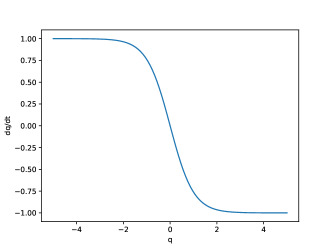
Figure 1: The stable manifold to the origin for the conservative system with $A=1/2,I=1$. Then $\ddot{q}=\tanh(q)\mathrm{sech}^{2}(q)$. This is given by the graph of $\dot{q}=-\tanh q$

3.1.2 Forced and damped model

The model in Equation (17) is now perturbed by a linear damping term and a time dependent forcing term, leading to the equation

$$I\ddot{q}=2A\tanh(q)\mathrm{sech}^{2}(q)-k\dot{q}+F(t),$$ (18)

where $k$ is a positive constant. Through the introduction of dimensionless variables $s=\sqrt{\frac{2A}{I}}t$, $x(s)=q(t)$, and using ^′ to denote $\frac{\mathrm{d}}{\mathrm{d}s}$, Equation (18) can be recast as

$$x^{\prime\prime}=\tanh(x)\mathrm{sech}^{2}(x)-\tilde{k}x^{\prime}+\tilde{F}(s)$$ (19)

where $\tilde{k},\tilde{F}$ represent the re-scaling of the damping and forcing terms. Equation (19) will now be the object of the study of this subsection, as it represents the qualitative dynamics of Equation (18). From now on tildes will be omitted, and we will use $k,F$ to denote the dimensionless parameters.

To approach this system using the methods outlined in Section 2, we introduce $y=x^{\prime}$ and the equations of motion become

$$\begin{pmatrix}x^{\prime}(s)\\ y^{\prime}(s)\end{pmatrix}=\begin{pmatrix}y(s)\\ \tanh(x(s))\mathrm{sech}^{2}(x(s))-ky(s)\end{pmatrix}+\begin{pmatrix}0\\ F(s)\end{pmatrix}.$$ (20)

In the case of $F=0$, Equation (20) has a unique hyperbolic steady state at $(0,0)$. Applying the terminology established in Section 2.1.1, the linearised system corresponding to Equation (20) is given by

$$\begin{pmatrix}u^{\prime}(s)\\ v^{\prime}(s)\end{pmatrix}=\begin{pmatrix}0&1\\ 1&-k\end{pmatrix}\begin{pmatrix}u(s)\\ v(s)\end{pmatrix}+\begin{pmatrix}0\\ F(s)\end{pmatrix}.$$ (21)

where $(u,v)$ denotes a small perturbation from $(0,0)$. This is a system of the form of Equation (5) with

$$\mathbf{A}=\begin{pmatrix}0&1\\ 1&-k\end{pmatrix}.$$

The origin is therefore a saddle point with eigenvalues $\lambda_{\pm}=\frac{-k\pm\sqrt{4+k^{2}}}{2}$ and eigenvectors $\mathbf{v}_{\pm}=(1,\lambda_{\pm})^{T}$. Letting $\mathbf{P}=(\mathbf{v}_{-},\mathbf{v}_{+})$ be the change of basis matrix to the eigenvectors, it can be shown that the system defined by Equation (21) is equivalent to the system:

$$\begin{pmatrix}y_{-}^{\prime}(s)\\ y_{+}^{\prime}(s)\end{pmatrix}=\begin{pmatrix}-1-\lambda_{-}^{2}&0\\ 0&1+\lambda_{+}^{2}\end{pmatrix}\begin{pmatrix}y_{-}(s)\\ y_{+}(s)\end{pmatrix}+\begin{pmatrix}-F(s)\\ F(s)\end{pmatrix}.$$ (22)

where $(u,v)^{T}=y_{-}\mathbf{v}_{-}+y_{+}\mathbf{v}_{+}$. Equation (22) has the same form as the two dimensional system in Section 2.1.1, and so can be solved using the general solution presented there and then transformed to the original coordinate system.

3.1.3 Results

The methods outlined in Sections 2.1.2 and 2.2.2 were applied to the system in Equation (20), using the linearised system given by (22) for the initial guess of the trajectories. For numerical simulations we choose $k=1$ or $3$, and $F(s)=0.1\cos(0.7s)-0.15\cos(2s)$.

In Figure 2 a hyperbolic trajectory for this forcing (and for two values of damping) is plotted together with the stable and unstable manifolds in the extended state space of $\mathbb{R}^{2}\times\mathbb{R}$.

A trajectory is deemed to cross the hyperbolic trajectory when it crosses the dividing manifold given by $x=x_{hyp}(t)$. This manifold consists of two parts: $y>y_{hyp}(t)$, which trajectories cross with $\dot{x}>0$; and $y<y_{hyp}(t)$, which trajectories cross with $\dot{x}<0$; this allows us to compare the direction of the crossing of a trajectory.

(a) $k=1$

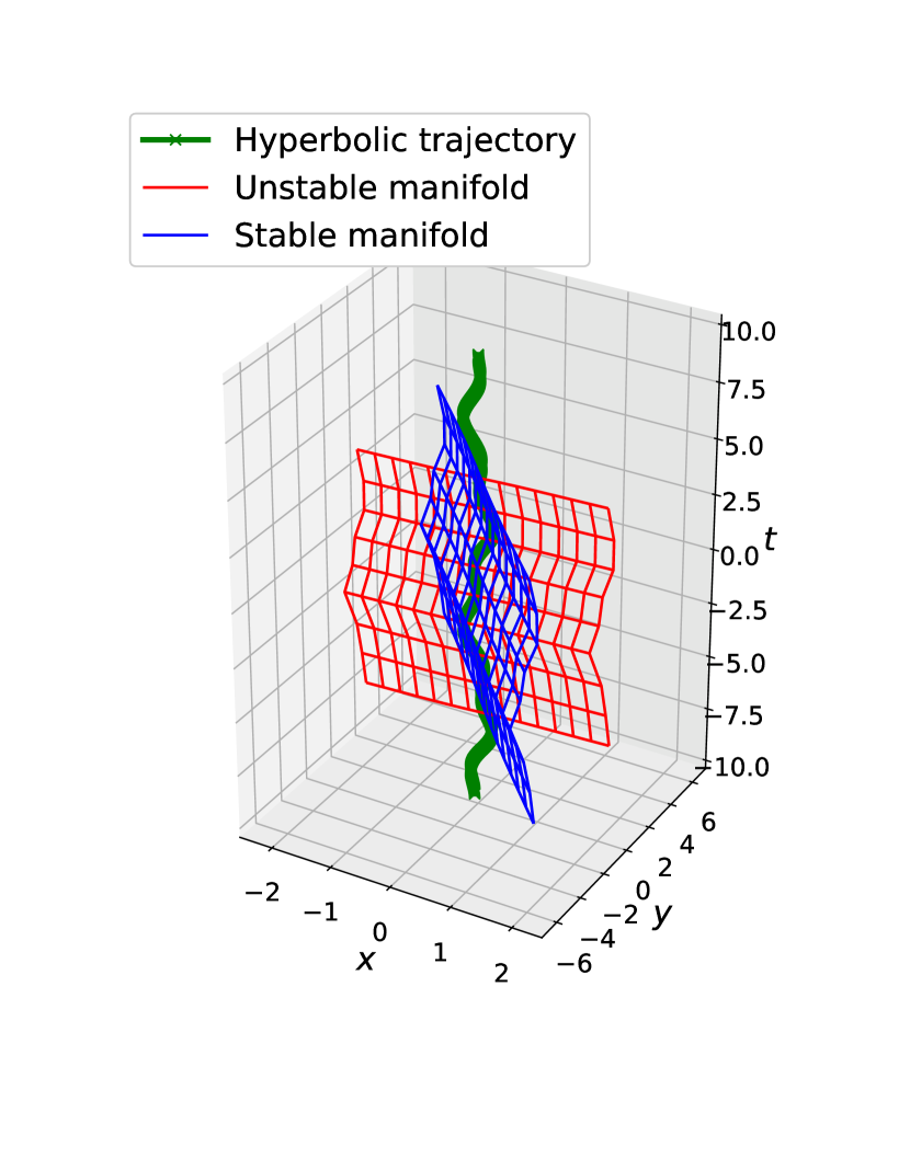
(b) $k=3$

Figure 2: The stable and unstable manifolds to the hyperbolic trajectory to $x^{\prime\prime}=\tanh(x)\mathrm{sech}^{2}(x)-kx^{\prime}+0.1\cos(0.7s)-0.15\cos(2s)$ for $k=1,3$..

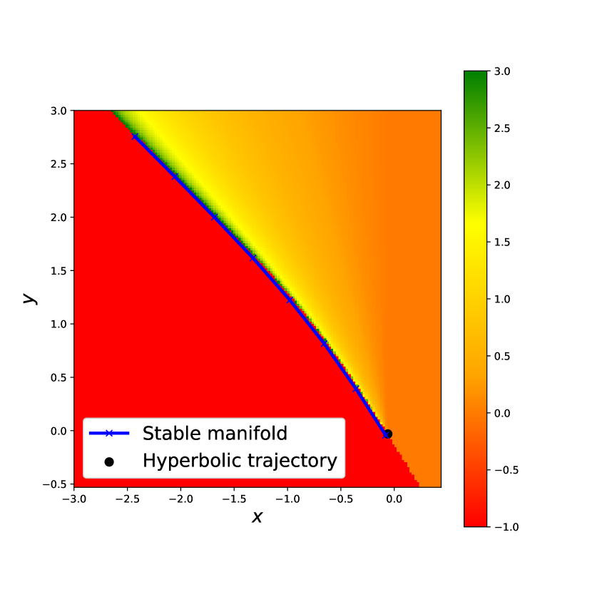
(a) $k=1$

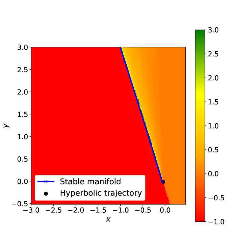
(b) $k=3$

Figure 3: A branch of the stable manifold is plotted in the plane $t=0$ and this is compared with a heat map of initial conditions coloured according to the time it takes to transition over the hyperbolic trajectory. The points which do not transition are assigned the value of $-1$ and appear as red. This is done for the systems $x^{\prime\prime}=\tanh(x)\mathrm{sech}^{2}(x)-kx^{\prime}+0.1\cos(0.7s)-0.15\cos(2s)$ with $k=1,3$.

3.2 Two DOF model

In this section, the methods outlined in Section 2 are applied to a qualitative roll-heave model from thompson1996suppression , to model ship motions.

3.2.1 Autonomous model

In the absence of damping or external forces acting on the ship, the system is taken to evolve according to

$$\begin{split}m\ddot{z}+h\left(z-\tfrac{1}{2}\gamma\phi^{2}\right)=0\\ I\ddot{\phi}+c\phi\left[1-\left(\phi/\phi_{v}\right)\right]\left[1+\left(\phi/\phi_{v}\right)\right]-h\gamma\phi\left(z-\tfrac{1}{2}\gamma\phi^{2}\right)=0\end{split}$$ (23)

which is Hamiltonian with Lagrangian

$$\mathcal{L}=\tfrac{1}{2}\left(I\dot{\phi}^{2}+m\dot{z}^{2}\right)-V(\phi,z)$$ (24)

where the potential is given by

$$V(\phi,z)=\frac{1}{2}c\phi_{v}^{2}\left[\left(\phi/\phi_{v}\right)^{2}-\frac{1}{2}\left(\phi/\phi_{v}\right)^{4}\right]+\frac{1}{2}h\left[z-\frac{1}{2}\gamma\phi^{2}\right]^{2}$$

To reduce the number of parameters, we introduce dimensionless quantities $x=z/z_{v},y=\phi/\phi_{v},s=\sqrt{\frac{c}{I}}t$, where $z_{v}=\tfrac{1}{2}\gamma\phi_{v}^{2}$. Following thompson1996suppression it is assumed that $\gamma^{2}=\frac{2c}{h\phi_{v}^{2}}$, and under these new variables the equations of motion become

$$\begin{split}x^{\prime\prime}+\tilde{h}(x-y^{2})+k_{x}x^{\prime}=\tilde{F}(s)\\ y^{\prime\prime}+y-xy+\tilde{D}(y^{\prime})=\tilde{M}(s)\end{split}$$ (25)

where $\tilde{h}=\frac{hI}{mc}$, $k_{x}=\frac{k_{z}\sqrt{c}}{m\sqrt{I}}$, $\tilde{F}(s)=\frac{I}{mcz_{v}}F\left(\sqrt{\frac{I}{c}}s\right)$, $\tilde{D}(v)=\frac{1}{c\phi_{v}}D\left(\phi_{v}\sqrt{\frac{c}{I}}v\right)$ $\tilde{M}(s)=\frac{1}{c\phi_{v}}M\left(\sqrt{\frac{I}{c}}s\right)$.

For the remainder of this paper only the rescaled system in Equation (25) will be studied, and all tildes will be dropped from the parameters and functions.

Using $v_{x}=x^{\prime},v_{y}=y^{\prime}$, the corresponding Lagrangian is now given by:

$$\mathcal{L}_{2}=T_{2}(v_{x},v_{y})-V_{2}(x,y)=\frac{1}{4h}(v_{x})^{2}+\frac{1}{2}(v_{y})^{2}-\frac{1}{2}\left(y^{2}+\frac{1}{2}x^{2}-xy^{2}\right)$$

An analysis of the conservative system corresponding to this Lagrangian is presented in naik2017geometry , and so we will not present a detailed analysis of the system here, however we shall briefly describe the geometry of the energy levels.

In the case where no external moments or forces are applied, Equation (25) possesses three equilibria, at $(0,0,0,0),(1,1,0,0),(1,-1,0,0)$. The energy of the system is given by

$$H(x,y,v_{x},v_{y})=\frac{1}{4h}(v_{x})^{2}+\frac{1}{2}(v_{y})^{2}+\frac{1}{2}\left(y^{2}+\frac{1}{2}x^{2}-xy^{2}\right)$$

The equilibria $(1,1,0,0),(1,-1,0,0)$ both have energy $H=\tfrac{1}{4}$ and the origin lies on the energy level $H=0$. For $0<E<\tfrac{1}{4}$ the energy level set $H=E$ consists of three disconnected regions, one a bounded neighbourhood of the origin in the position variables $x$ and $y$, the other two unbounded regions corresponding to regions of unbounded motion. For $E>\tfrac{1}{4}$ the energy level $H=E$ consists of a connected unbounded energy region which allows passage of the system from a neighbourhood of the $(x,y)=(0,0)$ to the region of unbounded motion.

In Figure 4 the Hill’s region is plotted for $H=0.2,0.3$. This is the projection of the energy level $H=h$ onto the $(x,y)$ plane and indicates where trajectories of the system can lie in the absence of forcing. The energy level is a circle bundle over these regions, with the circle representing the set of directions for the velocity, and which shrinks to a point on the boundary of the Hill’s region, which are called zero-velocity curves naik2017geometry . In the absence of forcing, trajectories cannot pass through the zero-velocity curves and so they serve to bound the motion of the system.

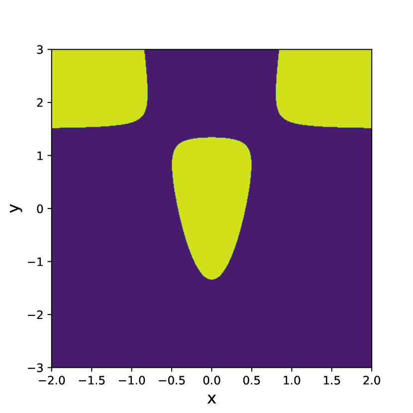
(a) $H=0.2$

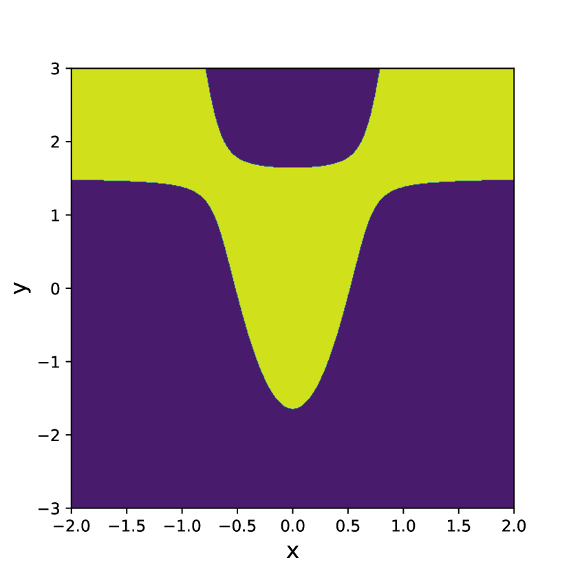
(b) $H=0.3$

Figure 4: The projection of the energy level onto the $(x,y)$ plane (Hill’s region) is coloured in yellow.

With the number of parameters now reduced it is easier to analyse the linearised system of equations for the autonomous system at the corresponding equilibria. Writing Equation (25) as a first order system of equations we define:

$$\mathbf{f}(x,y,v_{x},v_{y})=(v_{x},v_{y},-h(x-y^{2})-k_{x}v_{x},-y+xy-D(v_{y}))^{T}$$

and so Equation (25) is equivalent to

$$(x^{\prime},y^{\prime},v_{x}^{\prime},v_{y}^{\prime})^{T}=\mathbf{f}(x,y,v_{x},v_{y})$$

The linearisation of $\mathbf{f}$ about the saddle points $(1,\pm 1,0,0)$ is given by the matrix

$$D\mathbf{f}(1,\pm 1,0,0)=\begin{pmatrix}0&0&1&0\\ 0&0&0&1\\ -h&\pm 2h&-k_{x}&0\\ \pm 1&0&0&-k_{y,0}\end{pmatrix}$$

where $k_{y,0}=D^{\prime}(0)>0$. This has a characteristic polynomial at both saddle points of:

$$\chi(\lambda)=\lambda^{4}+(k_{x}+k_{y,0})\lambda^{3}+(k_{x}k_{y,0}+h)\lambda^{2}+hk_{y,0}\lambda-2h.$$ (26)

In general the roots to Equation (26) are best found numerically as the number of parameters are too high for the algebraic solutions to be practical.

For the purposes of demonstrating the qualitative nature of the model we shall take $k_{x}=k_{y,0}=k>0$. The eigenvalues are then given by:

$$\lambda_{1} =\frac{1}{2}\left(-k-\sqrt{k^{2}-\alpha}\right)$$

$$\lambda_{2} =\frac{1}{2}\left(-k+\sqrt{k^{2}-\alpha}\right)$$

$$\lambda_{3} =\frac{1}{2}\left(-k-\sqrt{k^{2}+\beta}\right)$$

$$\lambda_{4} =\frac{1}{2}\left(-k+\sqrt{k^{2}+\beta}\right)$$

where $\alpha=2h+2\sqrt{h}\sqrt{8+h}$ and $\beta=-2h+2\sqrt{h}\sqrt{8+h}$. It follows that the equilibrium is a saddle with one expanding direction. The eigenvectors for $D\mathbf{f}(1,1,0,0)$ are given by:

$$\mathbf{v}_{1} =\begin{pmatrix}\frac{k}{2}-\frac{1}{2}\sqrt{k^{2}-\alpha}\\ -\frac{\sqrt{h}}{8\sqrt{h}}\left(-k+\sqrt{k^{2}-\alpha}\right)-\frac{\sqrt{8+h}}{8\sqrt{h}}\left(k-\sqrt{k^{2}-\alpha}\right)\\ -\frac{h}{2}-\frac{1}{2}\sqrt{h}\sqrt{8+h}\\ 1\end{pmatrix}$$

$$\mathbf{v}_{2} =\begin{pmatrix}\frac{k}{2}+\frac{1}{2}\sqrt{k^{2}-\alpha}\\ -\frac{\sqrt{h}}{8\sqrt{h}}\left(-k-\sqrt{k^{2}-\alpha}\right)-\frac{\sqrt{8+h}}{8\sqrt{h}}\left(k+\sqrt{k^{2}-\alpha}\right)\\ -\frac{h}{2}-\frac{1}{2}\sqrt{h}\sqrt{8+h}\\ 1\end{pmatrix}$$

$$\mathbf{v}_{3} =\begin{pmatrix}\frac{k}{2}-\frac{1}{2}\sqrt{k^{2}+\beta}\\ -\frac{\sqrt{h}}{8\sqrt{h}}\left(-k+\sqrt{k^{2}+\beta}+\right)-\frac{\sqrt{8+h}}{8\sqrt{h}}\left(-k+\sqrt{k^{2}+\beta}\right)\\ -\frac{h}{2}+\frac{1}{2}\sqrt{h}\sqrt{8+h}\\ 1\end{pmatrix}$$

$$\mathbf{v}_{4} =\begin{pmatrix}\frac{k}{2}+\frac{1}{2}\sqrt{k^{2}+\beta}\\ -\frac{\sqrt{h}}{8\sqrt{h}}\left(-k-\sqrt{k^{2}+\beta}\right)-\frac{\sqrt{8+h}}{8\sqrt{h}}\left(-k-\sqrt{k^{2}+\beta}\right)\\ -\frac{h}{2}+\frac{1}{2}\sqrt{h}\sqrt{8+h}\\ 1\end{pmatrix}$$

The eigenvectors for $D\mathbf{f}(1,-1,0,0)$ can be found similarly. This gives different phase portraits depending on the sign of $k^{2}-\alpha$. In the case with no damping this would be negative, giving two eigenvalues on the imaginary axis. If the damping is small compared to the hydrostatic forces, we would expect that $k^{2}-\alpha<0$, and we assume that this holds for the remainder of the paper. In this case we can split $\mathbf{v}_{1}$ and $\mathbf{v}_{2}$ into the real and imaginary parts by:

$$\mathbf{v}_{1}=\mathbf{v}^{(1)}+i\mathbf{v}^{(2)},\quad\mathbf{v}_{2}=\mathbf{v}^{(1)}-i\mathbf{v}^{(2)}$$

where

$$\mathbf{v}^{(1)} =\left(\frac{k}{2},-\frac{1}{8\sqrt{h}}\left(-k\sqrt{h}+k\sqrt{8+h}\right),-\frac{h}{2}-\frac{1}{2}\sqrt{h}\sqrt{8+h},1\right)^{T}$$

$$\mathbf{v}^{(2)} =\left(-\frac{1}{2}\sqrt{-k^{2}+\alpha},-\frac{1}{8\sqrt{h}}\left(\sqrt{h}\sqrt{-k^{2}+\alpha}-\sqrt{8+h}\sqrt{-k^{2}+\alpha}\right),0,0\right)^{T}$$

In this case the homogeneous solution to the linearised IVP with initial values $\mathbf{x}_{0}=X_{1}\mathbf{v}^{(1)}+X_{2}\mathbf{v}^{(2)}+X_{3}\mathbf{v}_{3}+X_{4}\mathbf{v}_{4}$ is given by:

$$\begin{split}\mathbf{x}(t)=e^{-kt/2}\left(X_{1}\cos(\omega t)+X_{2}\sin(\omega t))\right)\mathbf{v}^{(1)}+\\ e^{-kt/2}\left(-X_{1}\sin(\omega t)+X_{2}\cos(\omega t))\right)\mathbf{v}^{(2)}+\\ e^{\lambda_{3}t}X_{3}\mathbf{v}_{3}+e^{\lambda_{4}t}X_{4}\mathbf{v}_{4}\end{split}$$ (27)

where $\omega=\tfrac{1}{2}\sqrt{\alpha-k^{2}}$. We can transform this back into the original coordinates by substituting the values for the eigenvectors.

3.2.2 Forced and damped model

As in the previous example, the framework established in Section 2 can be applied to the system in Equation (25). The solution to the corresponding linear system as in Equation (5) can be constructed as in Section 3.1.2, using Equation (27) to construct the $e^{t\mathbf{A}}\mathbf{X}_{0}$ term, and computing the integral $e^{t\mathbf{A}}\int_{0}^{t}e^{-s\mathbf{A}}(0,0,F(s),M(s))ds$ directly. This is best done by considering a coordinate system of eigenvectors for each saddle point, and in the case of periodic or quasi-periodic forcing, reduces to computing integrals of the form $\int_{0}^{t}e^{\lambda s}\cos(\omega_{f}s+\varepsilon)ds$ and $\int_{0}^{t}e^{\lambda s}\cos(\omega s)\cos(\omega_{f}s+\varepsilon)ds$.

In the case of this paper, the centre manifold was parameterised with a smooth interpolation $\iota_{C}$ as given in Section 2.3. For a specified time $t_{0}$, the intersection of the centre manifold to the hyperbolic trajectory $\mathbf{x}_{hyp}(\cdot)$ with the time slice $t=t_{0}$ has the linear approximation of $\mathbf{x}(t_{0})+\mathrm{Span}(\mathbf{D}\iota_{C}\cdot\mathbf{e_{1}},\mathbf{D}\iota_{C}\cdot\mathbf{e_{2}})$. To reduce complexity, the immersion for the stable manifold was used with $\iota_{C}(q_{1},q_{2},t)\approx\iota_{S}(q_{1},q_{2},0,t)$, where $q_{1},q_{2}$ denote the coordinates along the centre directions of the linearised system.

Having obtained the centre manifold, we then span it by two hypersurfaces of unidirectional flux, called a dividing surface. We consider crossing the dividing manifold in the appropriate direction as implying capsize. There is considerable arbitrariness to the dividing manifold, but they differ only in the time along a trajectory at which capsize is declared to take place.

A choice of dividing manifold corresponding to capsizing over $(1,\pm 1,0,0)$ was therefore taken as:

$$D_{M,\pm}=\{(x,y,v_{x},v_{y},t)\in\mathbb{R}^{5}:(x,y,v_{x},v_{y})-\mathbf{x}_{hyp,\pm}(t)\in\Pi_{t,\pm}\}$$ (28)

where $\mathbf{x}_{hyp,\pm}$ is the hyperbolic trajectory corresponding to the side of interest and

$$\Pi_{t,\pm}=\mathrm{Span}(\mathbf{D}\iota_{S,\pm}(e_{1}),\mathbf{D}\iota_{S,\pm}(e_{2}),\tfrac{1}{2}\mathbf{D}\iota_{S,\pm}(e_{3})+\tfrac{1}{2}\mathbf{v}_{4})$$

where $\mathbf{v}_{4}$ corresponds to the unstable eigenvector direction. Equation (28) can be interpreted as a smoothly varying family of affine subspace approximations to a dividing manifold, and so at each time it is straightforward to check which side of the dividing manifold a state is on, and hence it is simple to check when a trajectory does cross the dividing manifold, by expressing $D_{M,\pm}$ as $\{(\mathbf{x},t):L_{t}(\mathbf{x})=0\}$, where for each $t$, $L_{t}$ is an affine linear function.

The dividing manifold divides the state space into a capsized and a not capsized region, and the time to capsize of a trajectory is defined to be the time at which a trajectory crosses from one region into the other. By considering the sign of $L_{t}(\mathbf{x})$ for points known to lie in the capsize or non-capsize regions, these sides can be consistently categorised.

3.2.3 Results

The methods described in this paper were applied to the system (25) with external heave forcing $F=0$, model parameters $h=k=1$, with roll damping $D(v_{y})=kv_{y}$ and three cases of external moments:

$$M_{p}(t)=\cos(t),\ M_{q,1}(t)=\cos(\sqrt{2}t)+2\cos(4t),\ M_{q,2}(t)=\tfrac{1}{10}\left(\cos(\sqrt{2}t)+2\cos(4t)\right)$$ (29)

This system will have two hyperbolic trajectories of interest, corresponding to the saddle points $(1,\pm 1,0,0)$. These were first computed according to the method described in Section 2.1.2. Table 1 demonstrates the convergence of the method to the hyperbolic trajectory.

Forcing function	Number of iterations
	Negative trajectory	Positive trajectory
$M_{p}(t)$	16	17
$M_{q,1}(t)$	12	13
$M_{q,2}(t)$	5	6

Table 1: Iterations to find hyperbolic trajectories for the system given by (25), using the method outlined in Section 2.1.2.

The hyperbolic trajectories corresponding to the saddle points $(1,\pm 1,0,0)$ are plotted in $(x,y,t)$-space in Figure 5. Graphs of the components for the positive case as functions of $t$ are also shown in Figures 6, 7 and 8.

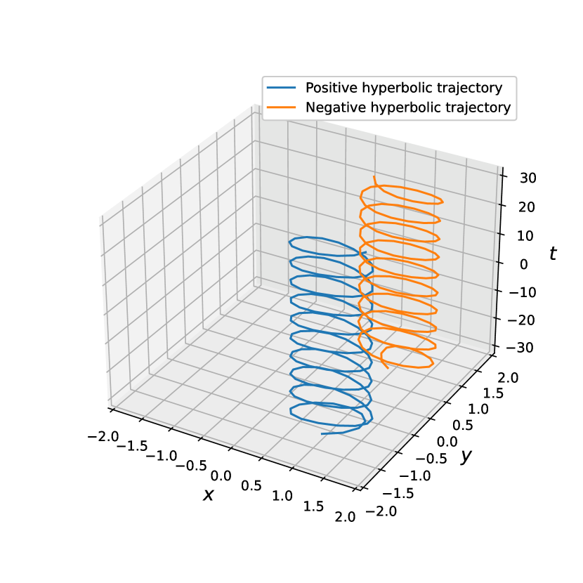
(a) Hyperbolic trajectories for $k=h=1$, $M(t)=M_{p}(t)=\cos(t)$

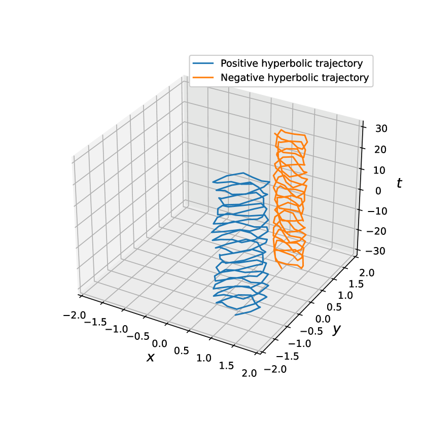
(b) Hyperbolic trajectories for $k=h=1$, $M(t)=M_{q,1}(t)=\cos(\sqrt{2}t)+2\cos(4t)$

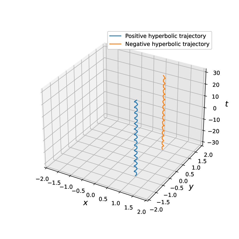
(c) Hyperbolic trajectories for $k=h=1$, $M(t)=M_{q,2}(t)=.1\cos(\sqrt{2}t)+.2\cos(4t)$

Figure 5: Hyperbolic trajectories to the two degree of freedom system plotted in $(x,y,t)$ space for the different forcing functions.

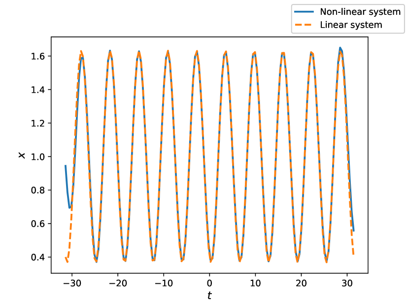
(a) Positive hyperbolic trajectory $x$ plotted against $t$

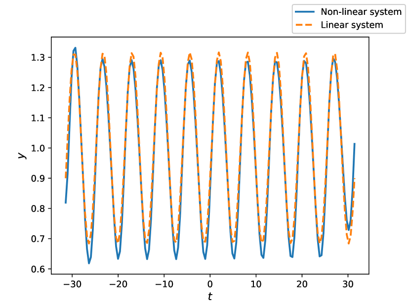
(b) Positive hyperbolic trajectory $y$ plotted against $t$

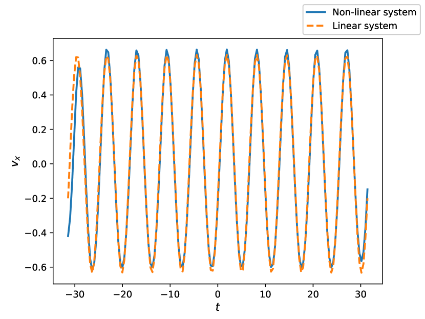
(c) Positive hyperbolic trajectory $v_{x}$ plotted against $t$

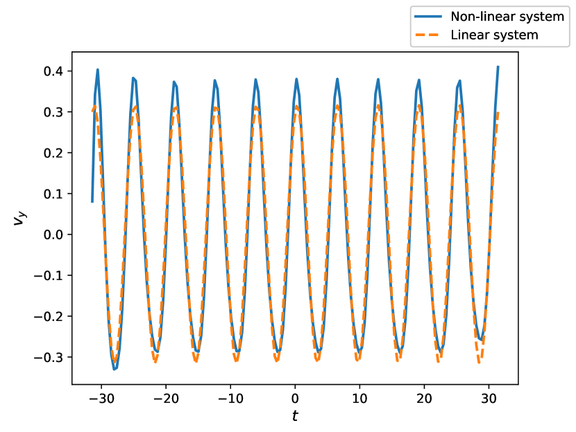
(d) Positive hyperbolic trajectory $v_{y}$ plotted against $t$

Figure 6: Positive hyperbolic trajectory for $k=h=1$, $M(t)=M_{p}(t)=\cos(t)$

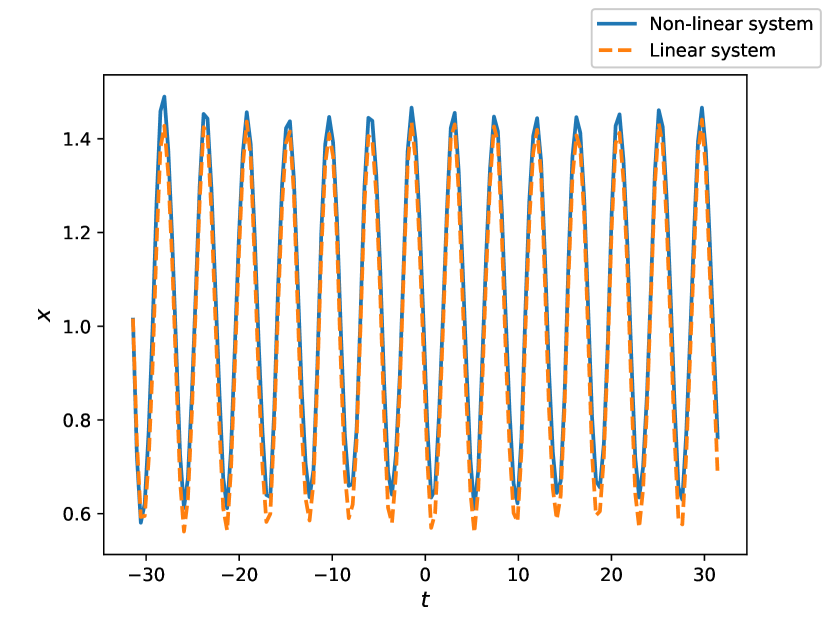
(a) Positive hyperbolic trajectory $x$ plotted against $t$

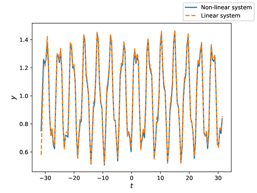
(b) Positive hyperbolic trajectory $y$ plotted against $t$

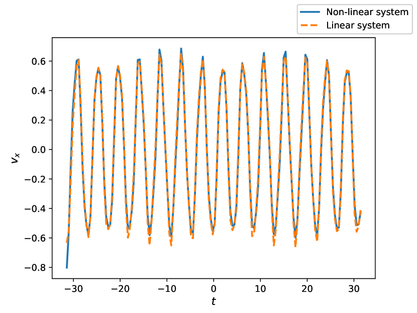
(c) Positive hyperbolic trajectory $v_{x}$ plotted against $t$

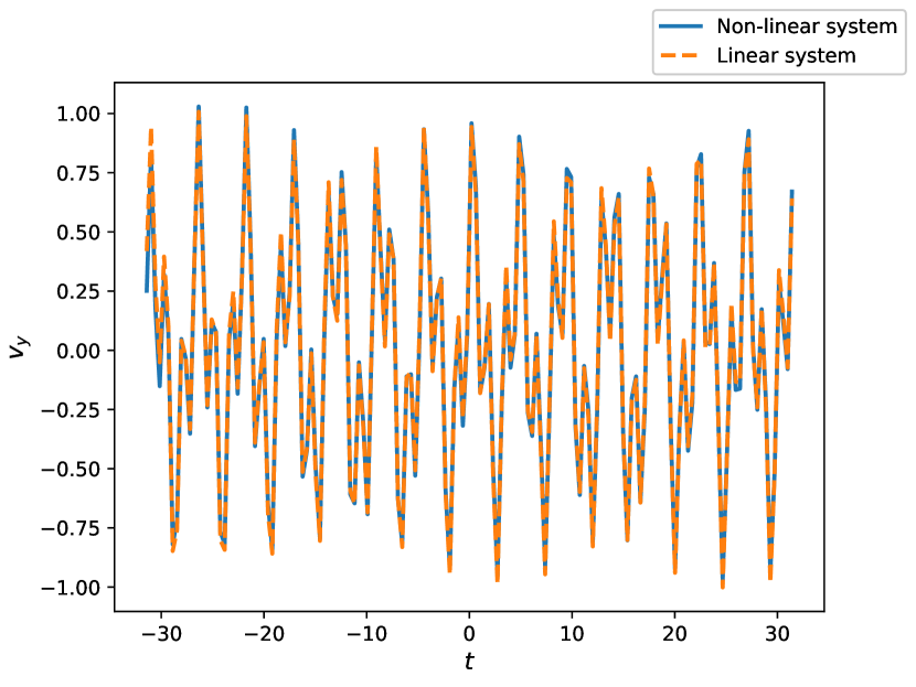
(d) Positive hyperbolic trajectory $v_{y}$ plotted against $t$

Figure 7: Positive hyperbolic trajectory for $k=h=1$, $M(t)=M_{q,1}(t)=\cos(\sqrt{2}t)+2\cos(4t)$

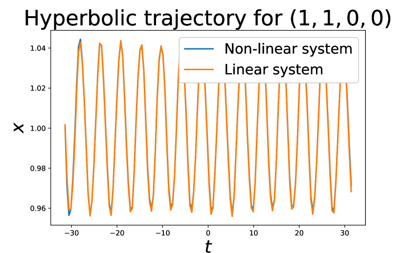
(a) Positive hyperbolic trajectory $x$ plotted against $t$

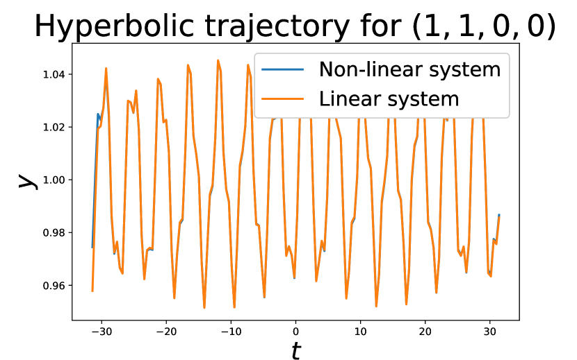
(b) Positive hyperbolic trajectory $y$ plotted against $t$

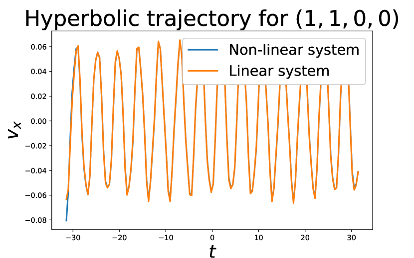
(c) Positive hyperbolic trajectory $v_{x}$ plotted against $t$

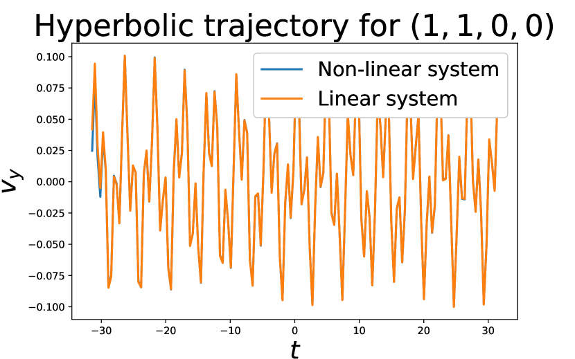
(d) Positive hyperbolic trajectory $v_{y}$ plotted against $t$

Figure 8: Positive hyperbolic trajectory for $k=h=1$, $M(t)=M_{q,2}(t)=.1\cos(\sqrt{2}t)+.2\cos(4t)$.

Similarly the stable and centre manifolds for these hyperbolic trajectories were computed according to the method described in Section 2.2.1 and 2.2.2.

It was found that the stable manifolds are given locally by graphs of the $v_{y}$ variable as a function of the $(t,x,y,v_{x})$ variables. Using an interpolation procedure the function $\tilde{v}_{y}(t,x,y,v_{x})$ was approximated, and for a given initial condition $(\mathbf{x},t)=(x,y,v_{x},v_{y},t)$ it was possible to classify it as capsize or non-capsize by considering the sign of $v_{y}-\tilde{v}_{y}(t,x,y,v_{x})$. This must be done for the stable manifold corresponding to each of the centre manifolds for each of the saddle points $(1,\pm 1,0,0)$.

If $(\mathbf{x},t)$ lies on a side corresponding to capsize over point $(1,\pm 1,0,0)$, then it is checked on which side of $D_{M,\pm}$. If it lies within the not-capsized region, the initial value problem with initial data $\mathbf{x}$ is solved until the solution crosses the dividing manifold. The time at which it does so is recorded as the time to capsize.

This methodology was applied to the system in Equation (25) with forcing from (29) and can be visualised in Figures 9, 10 and 11 where the stable manifold is plotted as a graph of the $v_{y}$ component against $(x,v_{x})$ with $y=0,t=0$ being fixed. On this plot a lattice of randomly selected points are also plotted and are coloured according to the time it takes for them to capsize, with the blue states not leading to capsize.

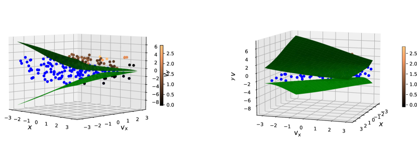
Figure 9: Initial conditions $(x,0,v_{x},v_{y})$ leading to capsize for $k=h=1$, and periodic forcing $M_{p}(t)=\cos(t)$ are plotted alongside the stable manifolds to the positive and negative hyperbolic trajectories. These points are coloured according to the time it takes for them to capsize, with the blue states not leading to capsize.

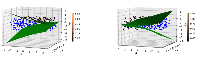
Figure 10: Initial conditions $(x,0,v_{x},v_{y})$ leading to capsize for $k=h=1$ and quasi-periodic forcing $M_{q,1}(t)=\cos(\sqrt{2}t)+2\cos(4t)$ are plotted alongside the stable manifolds to the positive and negative hyperbolic trajectories. These points are coloured according to the time it takes for them to capsize, with the blue states not leading to capsize.

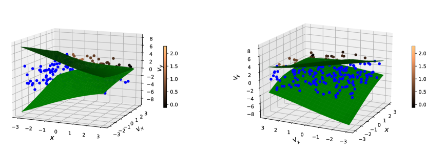
Figure 11: Initial conditions $(x,0,v_{x},v_{y})$ leading to capsize for $k=h=1$ and quasi-periodic forcing $M_{q,2}(t)=.1\cos(\sqrt{2}t)+.2\cos(4t)$ are plotted alongside the stable manifolds to the positive and negative hyperbolic trajectories. These points are coloured according to the time it takes for them to capsize, with the blue states not leading to capsize.

An initial roll angle was also considered. In Figure 12, the forcing considered is $M_{q,1}$ and there is an initial roll angle of $y=0.8$. The time to capsize and stable manifolds are plotted over this hypersurface, and it is possible to observe how this bias decreases the likelihood of capsizing over the negative roll angle.

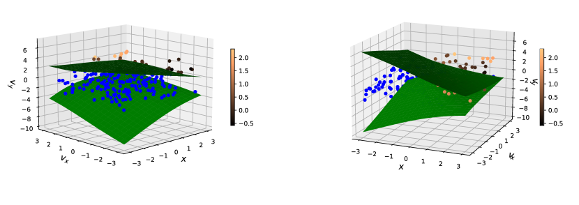
Figure 12: Initial conditions $(x,0.8,v_{x},v_{y})$ leading to capsize for $k=h=1$ and quasi-periodic forcing $M_{q,1}(t)=\cos(\sqrt{2}t)+2\cos(4t)$ are plotted alongside the stable manifolds to the positive and negative hyperbolic trajectories. These points are coloured according to the time it takes for them to capsize, with the blue states not leading to capsize. Comparing with Figure 10 we can observe how starting closer to $y=1$ increases the chance of capsizing over the positive side and decreases the likelihood capsizing over the negative side.

3.2.4 Integrity measure

The integrity measure provides a measure of the impact of external forcing on the stability of the ship. For our purposes the integrity measure is defined as the Lebesgue measure of initial conditions within the region $U=\{(x,y,v_{x},v_{y}):H(x,y,v_{x},v_{y})<\tfrac{1}{4},-1<y<1\}$ that do not lead to capsize. This region $U$ is contained within the basin of attraction of origin for the autonomous system, and so any decrease corresponds to an erosion of the basin of attraction for the upright trajectory. The region $U$ can be bounded by the rectangular region:

$$\begin{split}U\subset\{(x,y,v_{x},v_{y}):-1<x<1,-1<y<1,-\sqrt{h}<v_{x}<\sqrt{h},-\sqrt{2}<v_{y}<\sqrt{2}\}\\ =:C\end{split}$$

which makes it easier to sample points. The volume of $U$ can be computed analytically by evaluating a definite integral:

$$V_{U}=\int_{-1}^{1}dy\int_{H(x,y,v_{x},v_{y})<\tfrac{1}{4}}dxdv_{x}dv_{y}=\frac{163\pi\sqrt{2h}}{210}\approx 3.45h,$$

while the proportion of capsize points within is computed by Monte Carlo Integration.

Points are randomly selected within $C$ and if they lie within $U$ it is then classified as a capsize or non-capsize point by checking on which side of the stable manifold it lies. The probability of capsize is then evaluated by calculating the number of capsize points divided by the number of points within $U$.

Table 2 presents the integrity measure of each of the systems given by the forcing functions in (29).

Forcing function	Volume of safe region in $U$
0	3.45
$M_{p}(t)$	3.28
$M_{q,1}$	3.27
$M_{q,2}$	3.40

Table 2: Integrity measure for the system given by (25), with periodic, and quasi-periodic forcing functions defined in (29).

4 Discussion and conclusions

The approach outlined in this paper can be summarised as follows:

1. We examined the autonomous dissipative system and linearised the non-linear vector field about the saddle points.

2. For periodic and quasi-periodic forcing we derived the hyperbolic trajectories for the linearised system. Through the algorithm in Section 2.1.2, these were we found the hyperbolic trajectories for the non-linear system.

3. Applying The algorithm in Section 2.2.2 we computed a number of trajectories along the stable and centre manifold. These points were used to reconstruct the stable manifold by interpolating the immersion $\iota_{S}$ given by this algorithm.

4. By considering upon which side of the stable manifold an initial condition lies we determined the region of initial conditions which lead to transition over the saddle point/ centre manifold. We implemented this for a one degree of freedom system transition over an energy maximum and a two degree of freedom system modelling ship capsize.

5. For the latter system, we systematically computed the time to capsize using a dividing manifold, obtained using the stable manifolds. We also computed an integrity measure of the ship, to describe quantitatively how forcing affects the ship.

The main significance of this work is that it allows aperiodic forcing. It is expected that the method can be extended without major difficulty to systems with more degrees of freedom

Possible areas of extension are:

1. Applying this method to different forcing types, in particular to filtered white noise.

2. Incorporate probability distributions over forcing functions and initial conditions to obtain probability distributions of the time to capsize over initial conditions.

3. Extension to higher degrees of freedom. An energy based approach to modelling the 6 DOFs that includes configuration dependence of kinetic energy and potential energy and dissipative forcing due to waves was presented in nayfeh1974perturbation .

4. The establishment of control strategies, to keep the ship on the correct side of the stable manifolds.

5. Computation of a normally hyperbolic submanifold without requiring it to be a centre manifold for a hyperbolic trajectory. We used dissipation in this paper to guarantee existence of a hyperbolic trajectory corresponding to the saddle of the unforced system, and then to find its centre manifold, but in principle we could have computed a normally hyperbolic submanifold directly without having to find a hyperbolic trajectory. This will be important when extending to include neutral directions such as yaw, surge and sway.

Data availability statement

The code that supports some of the findings of this study is openly available at the following URL/DOI:https://github.com/AlexMcSD/ship-capsize-2022.

Acknowledgments This work was supported by the London Mathematical Society through a summer student bursary to the first author in 2022, with matched funding from the Mathematics Institute, University of Warwick.

Declarations

The authors declare they have no competing interests.

For the purpose of open access, the authors have applied a Creative Commons Attribution (CC-BY) licence to any Author Accepted Manuscript version arising from this submission.

References

- \bibcommenthead
- (1) Jaffé, C., Farrelly, D. & Uzer, T. Transition state in atomic physics. Physical Review A 60 (5), 3833 (1999) .
- (2) Eckhardt, B. Transition state theory for ballistic electrons. Journal of Physics A: Mathematical and General 28 (12), 3469 (1995). 10.1088/0305-4470/28/12/019 .
- (3) Komatsuzaki, T. & Berry, R. S. Dynamical hierarchy in transition states: Why and how does a system climb over the mountain? Proceedings of the National Academy of Sciences 98 (14), 7666–7671 (2001). 10.1073/pnas.131627698 .
- (4) Eyring, H. The activated complex in chemical reactions. The Journal of Chemical Physics 3 (2), 107–115 (1935) .
- (5) Wigner, E. The transition state method. Trans. Faraday Soc. 34, 29–41 (1938). 10.1039/TF9383400029 .
- (6) Wiggins, S., Wiesenfeld, L., Jaffé, C. & Uzer, T. Impenetrable barriers in phase-space. Phys. Rev. Lett. 86, 5478–5481 (2001). URL https://link.aps.org/doi/10.1103/PhysRevLett.86.5478. 10.1103/PhysRevLett.86.5478 .
- (7) Collins, P., Ezra, G. S. & Wiggins, S. Isomerization dynamics of a buckled nanobeam. Phys. Rev. E 86, 056218 (2012). 10.1103/PhysRevE.86.056218 .
- (8) Zhong, J., Virgin, L. N. & Ross, S. D. A tube dynamics perspective governing stability transitions: An example based on snap-through buckling. International Journal of Mechanical Sciences 149, 413–428 (2018). https://doi.org/10.1016/j.ijmecsci.2017.10.040 .
- (9) Virgin, L. N. Approximate criterion for capsize based on deterministic dynamics. Dynamics and Stability of Systems 4 (1), 56–70 (1989). 10.1080/02681118908806062 .
- (10) Thompson, J. M. T. & De Souza, J. R. Suppression of escape by resonant modal interactions: in shell vibration and heave-roll capsize. Proceedings of the Royal Society of London. Series A: Mathematical, Physical and Engineering Sciences 452 (1954), 2527–2550 (1996) .
- (11) Naik, S. & Ross, S. D. Geometry of escaping dynamics in nonlinear ship motion. Communications in Nonlinear Science and Numerical Simulation 47, 48–70 (2017) .
- (12) Jaffé, C. et al. Statistical theory of asteroid escape rates. Physical Review Letters 89 (1), 011101 (2002) .
- (13) Dellnitz, M. et al. Transport of mars-crossing asteroids from the quasi-hilda region. Phys. Rev. Lett. 94, 231102 (2005). URL https://link.aps.org/doi/10.1103/PhysRevLett.94.231102. 10.1103/PhysRevLett.94.231102 .
- (14) de Oliveira, H. P., Ozorio de Almeida, A. M., Damião Soares, I. & Tonini, E. V. Homoclinic chaos in the dynamics of a general bianchi type-ix model. Phys. Rev. D 65, 083511 (2002). 10.1103/PhysRevD.65.083511 .
- (15) Nayfeh, A. H., Mook, D. T. & Marshall, L. R. Nonlinear coupling of pitch and roll modes in ship motions. Journal of Hydronautics 7 (4), 145–152 (1973) .
- (16) Falzarano, J. M., Shaw, S. W. & Troesch, A. W. Application of global methods for analyzing dynamical systems to ship rolling motion and capsizing. International journal of bifurcation and chaos 2 (01), 101–115 (1992) .
- (17) Zhong, J. & Ross, S. D. Geometry of escape and transition dynamics in the presence of dissipative and gyroscopic forces in two degree of freedom systems. Communications in Nonlinear Science and Numerical Simulation 82, 105033 (2020). 10.1016/j.cnsns.2019.105033 .
- (18) Hernandez, R., Uzer, T. & Bartsch, T. Transition state theory in liquids beyond planar dividing surfaces. Chemical Physics 370 (1-3), 270–276 (2010) .
- (19) Pollak, E. & Talkner, P. Reaction rate theory: What it was, where is it today, and where is it going? Chaos: An Interdisciplinary Journal of Nonlinear Science 15 (2), 026116 (2005). 10.1063/1.1858782 .
- (20) Craven, G. T., Junginger, A. & Hernandez, R. Lagrangian descriptors of driven chemical reaction manifolds. Physical Review E 96 (2) (2017). 10.1103/PhysRevE.96.022222 .
- (21) Bishnani, Z. & MacKay, R. S. Safety criteria for aperiodically forced systems. Dynamical Systems: An International Journal 18 (2), 107–129 (2003) .
- (22) Fenichel, N. Asymptotic stability with rate conditions. Indiana University Mathematics Journal 23 (12), 1109–1137 (1974) .
- (23) Fenichel, N. Asymptotic stability with rate conditions, ii. Indiana University Mathematics Journal 26 (1), 81–93 (1977) .
- (24) Bujorianu, M. L., MacKay, R. S., Grafke, T., Naik, S. & Boulougouris, E. A new stochastic framework for ship capsizing. arXiv preprint arXiv:2105.05965 (2021) .
- (25) MacKay, R. Flux over a saddle. Physics Letters A 145 (8), 425–427 (1990). https://doi.org/10.1016/0375-9601(90)90306-9 .
- (26) Kinney, W. On the unstable rolling motions of ships resulting from nonlinear coupling with pitch including the effect of damping in roll 3 (University of California, Institute of Engineering Research, 1961).
- (27) Paulling, J. R. R. & Rosenberg, R. M. On unstable ship motions resulting from nonlinear coupling. Journal of Ship Research 3 (02), 36–46 (1959) .
- (28) Froude, W. Remarks on mr. scott russell’s paper on rolling. Transactions of the Institute of Naval Architects 4 (4), 232–275 (1863) .
- (29) Kuznetsov, S. P. Hyperbolic chaos (Springer, 2012).
- (30) Madrid, J. A. J. & Mancho, A. M. Distinguished trajectories in time dependent vector fields. Chaos: An Interdisciplinary Journal of Nonlinear Science 19 (1) (2009) .
- (31) Parker, T. S. & Chua, L. O. Practical numerical algorithms for chaotic systems (Springer Science & Business Media, 2012).
- (32) Jolly, M. S. & Rosa, R. Computation of non-smooth local centre manifolds. IMA Journal of Numerical Analysis 25 (4), 698–725 (2005) .
- (33) Mancho, A. M., Small, D., Wiggins, S. & Ide, K. Computation of stable and unstable manifolds of hyperbolic trajectories in two-dimensional, aperiodically time-dependent vector fields. Physica D: Nonlinear Phenomena 182 (3-4), 188–222 (2003) .
- (34) Nayfeh, A. H., Mook, D. T. & Marshall, L. R. Perturbation-energy approach for the development of the nonlinear equations of ship motion. Journal of Hydronautics 8 (4), 130–136 (1974) .