Asymptotic Velocity Bounds for Random Walks in Random Environments with Two Kinds of Site

Abstract

This paper studies random walks in i.i.d. random environments on $\mathbb{Z}^{d}$ when there are two basic types of vertices, which we call “blue” and “red,” with drifts in different directions. We introduce a method of studying these walks that compares the expected amount of time spent at a specific site on the event that the site is red with the expected amount of time spent there on the event that the site is blue. An advantage of this method is that it produces explicit bounds on the asymptotic velocity of the walk. We use the method to recover an early result of Kalikow [3], but with new explicit bounds on the asymptotic velocity. Next, we consider a model where the vast majority of sites are blue, and blue sites satisfy a non-nestling assumption, but red sites break the non-nestling assumption and are permitted to be highly pathological (for instance, red sites are allowed to give the walk zero probability of stepping in all but two directions). We show that if the red sites satisfy a certain uniform ellipticity assumption in two fixed directions, then making red sites unlikely enough can push the asymptotic velocity of the walk arbitrarily close to the bounds that come from the non-nestling assumption on the blue sites, if all sites were blue. Significantly, the required proportion $p^{*}$ of blue sites does not depend on the distribution of red sites, except through the uniform ellipticity assumption in two directions. Our proof is based on a coupling technique, where two walks run in environments that are the same everywhere except at one vertex. They decouple when they hit that vertex, and our proof is driven by bounds on how long it takes to recouple. We then show that the i.i.d. assumption in the theorem is necessary by providing a counterexample to the statement of the theorem with the i.i.d. assumption removed. We conclude with open questions.

1 Introduction

Random walks in random environments on $\mathbb{Z}^{d}$ are much harder to understand when $d\geq 2$ than when $d=1$. The model involves a random Markov chain with $\mathbb{Z}^{d}$ as the state space. A typcial assumption is that nearest-neighbor transition probability vectors at individual states are drawn in an i.i.d. way according to some underlying distribution. For instance, in [3], S. Kalikow presented the following i.i.d. two-vertex model: Fix $p\in(0,1)$ and positive probability vectors $<b_{1},b_{2},b_{3},b_{4}>$ and $<r_{1},r_{2},r_{3},r_{4}>$. Say that all sites in $\mathbb{Z}^{2}$ are independently “blue” with probability $p$ and “red” with probability $1-p$. Then, letting $e_{1},e_{2},e_{3},e_{4}$ respectively denote the “right,” “up,” “left,” and “down,” axis unit vectors, say that a walk ${\bf X}=(X_{n})_{n=0}^{\infty}$ steps in direction $e_{i}$ from a blue site with probability $b_{i}$, and from a red site with probability $r_{i}$.

$P(\text{blue})=p$		$P(\text{red})=1-p$
$P(\text{blue})=.999$		$P(\text{red})=.001$

Figure 1: Kalikow’s two-vertex model is depicted on the top. On the bottom is depicted the two-vertex model with the specific vertices Kalikow gave at the beginnng of [3].

The paper [3] opens rather provocatively with the following question: If $r_{2}=r_{4}=b_{2}=b_{4}=\frac{1}{4}$ (so that there is deterministically no vertical drift at any site and all vertical step probabilities are moderate), if $b_{1}=\frac{.999}{2}$, $b_{3}=\frac{.001}{2}$, $r_{1}=\frac{.499}{2}$, if $r_{3}=\frac{.501}{2}$ (so that there is a very strong rightward drift at blue sites and a very mild leftward drift at red sites), and if $p=.999$ (so that sites are overwhelmingly likely to be blue), then can one prove that the walk is almost surely transient to the right?

Although an affirmative answer certainly appears obvious, [3] takes a good deal of work to actually provide a proof, which comes as a result of showing that the model satisfies a criterion which has since come to be known as “Kalikow’s criterion.”

Theorem 1.

Suppose

$$\frac{p(b_{1}-b_{3})}{(1-p)(r_{3}-r_{1})}>M:=\max\left\{\frac{b_{i}}{r_{i}};i=1,2,3,4\right\}.$$ (1)

Then

1. the walk is transient to the right—that is, $\lim_{n\to\infty}X_{n}\cdot e_{1}=\infty$, almost surely;

2. The walk is ballistic; in fact, with probability 1,

   $$v:=\lim_{n\to\infty}\frac{X_{n}\cdot e_{1}}{n}\geq\frac{p(b_{1}-b_{3})-(1-p)M(r_{3}-r_{1})}{p+(1-p)M}.$$ (2)

Part (a) is proven in [3] as the Corollary to Theorem 1 (Theorem 1 proves the result under a more general, but non-explicit criterion known as “Kalikow’s Criterion.”). Sznitman and Zerner [7] proved that under Kalikow’s criterion, the walk is ballistic (has nonzero limiting speed). The paper [11] expressed the asymptotic velocity of models satisfying Kalikow’s condition in terms of Lyapunov exponents associated with the walk. The explicit bounds in (2) are new.

To understand some implications and limits of Theorem 1, consider the following model, where all vertical steps deterministically have probability $\frac{1}{4}$, blue sites have a moderate drift of $.1$ to the right, while at a red site, the probability of stepping to the right is $\varepsilon$.

$P(\text{blue})=p$		$P(\text{red})=1-p$

Figure 2: The case described in Theorem 2

Here, if $\varepsilon$ is small, then the $M$ in (1) is large, requiring $p$ to be close to 1 in order to satisfy (1). Indeed, asymptotically, $p$ must be at least $1-\frac{2}{3}\varepsilon$.

A goal of the present paper is to show transience to the right and ballisticity under milder assumptions that do not require $p$ to be taken arbitrarily close to 1. Indeed, we show that for sufficiently large (but fixed) $p$, $\varepsilon$ can be taken as small as one wishes—including 0—and transience to the right will hold, with a positive lower bound on the velocity that is uniform in $\varepsilon$ and that can be made arbitrarily close to 0.1, the strength of the rightward drift at blue sites.

Theorem 2.

Consider the i.i.d. two-vertex model where $b_{2}=b_{4}=r_{2}=r_{4}=\frac{1}{4}$, $b_{1}=.3$, $b_{3}=.2$, $r_{1}=\varepsilon$, and $r_{3}=\frac{1}{2}-\varepsilon$. For all $\delta>0$, there exists a $p^{*}\in(0,1)$ such that whenever $p>p^{*}$, the almost-sure limiting speed $\lim_{n\to\infty}\frac{X_{n}\cdot e_{1}}{n}$ is at least $0.1-\delta$.

Remark.

An analogous result would be false in one dimension. If blue sites send the walker to the right with probability $b_{1}>\frac{1}{2}$ and to the left with probability $b_{2}=1-b_{1}$, and red sites send the walker to the right with probability $\varepsilon$ and left with probability $1-\varepsilon$, then the results of [6] imply that for any fixed $b_{1},p\in(0,1)$, the walk can be made transient to the left by taking $\varepsilon$ sufficiently small. However, this is due to the fact that a walk that is transient to the right must go through every vertex; there is no way to “walk around” a bad vertex. In higher dimensions, this is no longer the case.

We prove Theorem 2 as a special case of the more general Theorem 3, which requires more notation to state. We formally introduce the model and state the theorem in section 1.1. We describe the main proof ideas in section 1.1. Section 2 gives a criterion for directional transience and ballisticity, which will be used both for Theorem 3 and Theorem 1. Section 4 proves Theorem 3. Section 5 shows the necessity of the i.i.d. assumption in Theorem 3 by providing a non-i.i.d. counterexample with good mixing properties for any $p\in(0,1)$ where blue and red sites are as described in Theorem 2 but where the walk does not have positive speed in direction $e_{1}$. Section 3 proves theorem 1. Section 6 concludes by asking some open questions.

1.1 Model and main result statement

Let $\mathcal{N}=\{e_{1},\ldots,e_{2d}\}$ be the nearest neighbors of $0$, with $e_{i+d}=-e_{i}$, $1\leq i\leq d$. Let

$$\mathcal{M}_{1}(\mathcal{N})=\left\{\xi:\mathcal{N}\to[0,1]:\sum_{i=1}^{2d}\xi(e_{i})=1\right\}$$

be the set of probability vectors on $\mathcal{N}$, and let

$$\Omega:=\prod_{x\in\mathbb{Z}^{d}}\mathcal{M}_{1}(\mathcal{N}):=\{(\omega^{x})_{x\in\mathbb{Z}^{d}}:\omega^{x}\in\mathcal{M}_{1}(\mathcal{N})\text{ for all }x\in\mathbb{Z}^{d}\}.$$

We refer to an element $\omega=(\omega^{x})_{x\in\mathbb{Z}^{d}}$ as an environment on $\mathbb{Z}^{d}$. If $X\subset\mathbb{Z}^{d}$, then let $\omega^{X}:=(\omega^{x})_{x\in X}$.

For a given environment $\omega$ and $x\in\mathbb{Z}^{d}$, we can define $P_{\omega}^{x}$ to be the measure on $(\mathbb{Z}^{d})^{\mathbb{N}_{0}}$ (with the natural sigma field) giving the law of a Markov chain $(X_{n})_{n=0}^{\infty}$ started at $x$ with transition probabilities given by $\omega$. That is, $P_{\omega}^{x}(X_{0}=x)=1$, and for $n\geq 1$, $y\in V$, $P_{\omega}^{x}(X_{n+1}-X_{n}=y|X_{0},\ldots,X_{n})=\omega^{X_{n}}(y)$ almost surely.

Rather than describe a model with only two types of vertices, we generalize to allow for two classes of vertices. We will let “blue” vertices have transition probability vectors distributed according to one measure $\mu_{b}$, and “red” vertices have transition probability vectors distributed according to another measure $\mu_{r}$. In order to keep track of which sites are blue and red, we will describe the notion of a tagged environment, which keeps track of which sites are blue and which are red as well as their transition probability vectors.

Let

$$\Upsilon:=\{\text{blue},\text{red}\}^{\mathbb{Z}^{d}}:=\{(\upsilon(x))_{x\in\mathbb{Z}^{d}}:\upsilon(x)\in\{\text{blue},\text{red}\}\text{ for all }x\in\mathbb{Z}^{d}\}.$$

be the set of “pre-environments,” and let

$$\boldsymbol{\Omega}:=\Upsilon\times\Omega$$

be the set of “tagged environments”—that is, environments where each site is assigned a color as well as a set of transition probabilities. We refer to a generic element $(\upsilon,\omega)$ of $\boldsymbol{\Omega}$ as $\boldsymbol{\omega}$.

Now if we give $\mathcal{M}_{1}(\mathcal{N})$ the topology of weak convergence and $\{\text{blue},\text{red}\}$ the discrete topology, we can let $\boldsymbol{\mathcal{F}}_{\mathbb{Z}^{d}}$ be the Borel sigma field on $\boldsymbol{\Omega}$.

Let ${\bf P}$ be a probability measure on $(\boldsymbol{\Omega},\boldsymbol{\mathcal{F}}_{\mathbb{Z}^{d}})$. For a given $x\in\mathbb{Z}^{d}$, we let $\mathbb{P}^{x}={\bf P}\times P_{\omega}^{x}$ be the measure on $\boldsymbol{\Omega}\times(\mathbb{Z}^{d})^{\mathbb{N}_{0}}$ induced by both ${\bf P}$ and $P_{\omega}$. That is, for measurable events $A\subset\boldsymbol{\Omega},B\subset(\mathbb{Z}^{d})^{\mathbb{N}_{0}}$,

$$\mathbb{P}^{x}(A\times B)=\int_{A}P_{\omega}^{x}(B){\bf P}(d\boldsymbol{\omega})$$ (3)

In particular, $\mathbb{P}^{x}(\boldsymbol{\Omega}\times B)={\bf E}\left[P_{\omega}^{x}(B)\right]$. For convenience, we commit a small abuse of notation by using $\mathbb{P}^{x}$ to refer both to the measure we’ve described on $\boldsymbol{\Omega}\times(\mathbb{Z}^{d})^{\mathbb{N}_{0}}$ and also to its marginal $\mathbb{P}^{x}(\boldsymbol{\Omega}\times\cdot)$ on $(\mathbb{Z}^{d})^{\mathbb{N}_{0}}$. We call a measure $P_{\omega}^{x}$ on $(\mathbb{Z}^{d})^{\mathbb{N}_{0}}$ a quenched measure of a random walk in random environment on $\mathbb{Z}$ started at $x$, and we call the measure $\mathbb{P}^{x}$ the annealed measure.

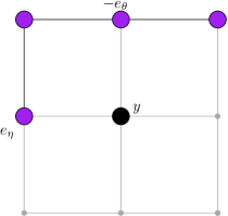
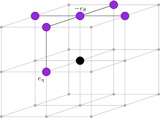
Say $e_{1},e_{2},\ldots,e_{2d}$ are the nearest neighbors of the origin, with $e_{i}=-e_{d+i}$ for $1\leq i\leq d$.

Let $\mu_{b}$ and $\mu_{r}$ be two probability measures on $\mathcal{M}_{1}(\mathcal{N})$ with the following properties.

1. Both $\mu_{b}$ and $\mu_{r}$ are supported on “nearest-neighbor” vectors—vectors that are zero away from the $2d$ nearest neighbors of the origin.

2. $\mu_{b}$ satisfies a uniform ellipticity assumption; there exists $\kappa>0$ such that with $\mu_{b}$-probability 1, all $2d$ neighbors of the origin have component at least $\kappa$.

3. $\mu_{b}$ satisfies the following strict non-nestling assumption: there is a unit vector $\vec{u}\in S^{d-1}$ and a $v_{1}>0$ such that $\mu_{b}$–almost surely, $\sum_{i=1}^{2d}\xi(e_{i})e_{i}\cdot\vec{u}\geq v_{1}>0$.

4. $\mu_{r}$ satisfies the following “two-direction” uniform ellipticity assumption: there exists $\kappa>0$ and two distinct values $\eta,\theta\in\{1,\ldots,d\}$ with $|\eta-\theta|\notin\{0,d\}$ (i.e., the vectors associated with $e_{\eta}$ and $e_{\theta}$ are orthogonal) such that with $\mu_{r}$-probability 1, the $e_{\eta}$ and $e_{\theta}$-components of the random probability vector are each at least $\kappa$.

Now let $p\in(0,1)$. Let ${\bf P}$ be the measure on $\boldsymbol{\Omega}$ such that

1. The pairs $(\upsilon(x),\omega^{x})$ are i.i.d.;

2. For each $x\in\mathbb{Z}^{d}$, $\upsilon(x)=\text{blue}$ with probability $p$, and $\upsilon(x)=\text{red}$ with probability $1-p$.

3. Conditioned on $\upsilon(x)=\text{blue}$, the law of $\omega^{x}$ is $\mu_{b}$;

4. Conditioned on $\upsilon(x)=\text{red}$, the law of $\omega^{x}$ is $\mu_{r}$.

Note that Kalikow’s two-vertex model is simply the special case where $d=2$ and where $\mu_{b}$ and $\mu_{b}$ are degenerate measures, each supported on one probability vector with all positive entries.

We are now able to state our main result, a more general version of Theorem 2.

Theorem 3.

For all $\varepsilon>0$, there exists $p^{*}<1$, depending only on $\varepsilon$, $d$, $v_{1}$, and $\kappa$, such that if $p>p^{*}$, then $\liminf_{n\to\infty}\frac{X_{n}\cdot\vec{u}}{n}\geq v_{1}-\varepsilon$, $\mathbb{P}^{0}$–almost surely.

Note that the value of $p^{*}$ depends on the distribution $\mu_{r}$ only through $\kappa$. In other words, one can bring the speed of the walk in direction $e_{1}$ arbitrarily close to $v_{1}$ simply by controlling how rare the exceptional sites are, without regard for what the exceptional sites look like, aside from the uniform ellipticity in two of the $2d$ directions.

1.2 Main proof ideas

Let us describe the main ideas of the proofs of both Theorem 1 and Theorem 3. We define functions for a walk ${\bf X}=(X_{n})_{n=0}^{\infty}$. For a vertex $x\in\mathbb{Z}^{d}$, define the hitting time and positive hitting time respectively as

$$H_{x}({\bf X}):=\inf\{n\geq 0:X_{n}=x\}\qquad\text{and}\qquad\tilde{H}_{x}({\bf X}):=\inf\{n>0:X_{n}=x\}.$$

and the local time

$$N_{x}({\bf X}):=\#\{n\geq 0:X_{n}=x\}.$$

For a $T\in\mathbb{N}$, define the truncated local time

$$N_{x}^{T}({\bf X}):=\#\{0\leq n\leq T:X_{n}=x\}.$$

As is typical with hitting times and other functions of a walk, we supress the argument in the above functions when the walk referred to is clear from the context. The function $x\mapsto\mathbb{E}^{0}[N_{x}]$ is the annealed Green’s function, and a function $x\mapsto\mathbb{E}^{0}[N_{x}^{T}]$ is a truncated annealed Green’s function.

The method of this proof is to examine the truncated, annealed Red’s function and Blue’s function given respectively by

$$\mathbb{E}^{0}\left[N_{x}^{T}\mathbbm{1}_{\{x\text{ is red}\}}\right]\quad\quad\quad\text{and}\quad\quad\quad\mathbb{E}^{0}\left[N_{x}^{T}\mathbbm{1}_{\{x\text{ is blue}\}}\right].$$

We show that that the truncated Red’s function as a multiple of the truncated Blue’s function can be bounded arbitrarily close to 0, uniformly in $x$ and in $T$, by making $p$ large enough. Summing over all $x\in\mathbb{Z}^{d}$, this implies that for any time $T$, the walk typically spends a very high proportion of the time from 0 to $T$ at blue sites.

This “typical” behavior, which is given in terms of expectations, becomes an almost-sure statement in the presence of a deterministic limiting velocity. The arguments of [7] yield an almost sure limiting velocity, but one which may be random, supported on two points, in the case where a 0-1 law for directional transience does not hold. However, because the bound on the truncated Red’s funciton is uniform for all $x\in\mathbb{Z}^{d}$, we may sum over all $x$ on one side of a hyperplane far form the origin. This argument essentially shows that conditioning on the walk’s being transient in one direction or the other does not affect the bound on the proportion of time it spends at red sites, and therefore does not affect the bound on the expected displacement after a large number of steps. This results in a contradiction and proves the 0-1 law. The result of this work is Theorem 4, which is used in the proof of Theorems 1 and 3.

For the proof of Theorem 1, our comparison of the truncated Red’s function and Blue’s function comes from exact expressions of ratios of these functions that involve probabilities of hitting and then returning to a site $x$, conditioned on the first step away from $x$. The main calculation is brief, but we need to truncate the walk at a random (geometric) time $\tau$, rather than a fixed $T$, in order to make it work. This geometric truncation is inspired by [4].

Proving Theorem 3 is more difficult, and for this we use a coupling technique. Red sites are typically surrounded by blue sites. To show that a walk does not spend too much time on such red sites, we can couple two walks in environments that exactly the same except at site $x$, which is blue in one environment and red in the other. The two walks decouple whenever they hit $x$. Then the particle in the environment for which $x$ is blue freezes, while the particle for which $x$ is red will only hit $x$ at most a geometric number of times before it uses the blue sites surrounding $x$ to navigate to the point adjacent to $x$ where the first particle is waiting. At this time, they recouple and continue as before. This allows us to bound, for these two environments, the expected amount of time spent at a red site surrounded by blue sites in terms of the amount spent at the blue site surrounded by blue sites, irrespective of the rest of the environment. Then, by taking $p$ large enough, we can make the environments rare enough that under the annealed measure, the walk is expected to spend much more time in blue sites than in red sites surrounded by blue sites.

Of course, not every red site is completely surrounded by blue sites, and if $x$ is in a cluster of red sites, the above argument does not work directly. But we can use a similar argument to compare how much time the walk spends at sites $x$ that are in red clusters of various sizes, showing that the amount of time spent in a cluster of size $m$ decreases exponentially fast in $m$. To do this, we compare walks in two environments that are both red at $x$ and are the same everywhere except for a carefully chosen point $y$ at the boundary of a cluster containing $x$. By the choice of $y$, enough sites near $y$ are blue that the above argument can go through, and then we can bound the amount of time spent at $x$, and we can show, again by taking $p$ large enough, that the walker is expected to spend much more time at sites $x$ that are in red clusters of size $m-1$ than at sites $x$ in red clusters of size $m$. We then sum over all clusters and then invoke the comparison between clusters of size 1 (where only $x$ is red) and clusters of size 0 (where $x$ itself is blue) to get the desired result.

Acknowledgments

The author thanks his advisor, Jonathon Peterson, for useful conversations, and especially for suggesting the geometric killing used in the proof of Theorem 1. Some of the work on this paper, including the initial idea, was supported through NSF grant DMS-2153869. The author is grateful to Leonid Petrov for providing this support.

2 A criterion for directional transience and ballisticity

In this section, we give a criterion for directional transience and ballisticity in terms of truncated Blue’s and Red’s functions. The criterion will be used in the proofs of both Theorem 3 and Theorem 1. Because the latter proof requires truncating at a random time, we give the criterion in terms of a geometric random variable $\tau$ rather than a fixed $T$.

We also describe a condition that will replace a tradicional ellipticity assumption.

1. The probability $p$ and the measure $\mu_{r}$ are such that with ${\bf P}$-probability 1, the Markov chain induced by $\omega$ has only one infinite communicating class, and it is reachable from every site.

This is clearly satisfied under the traditioanl ellipticity assumption where $\mu_{r}$ is supported on vectors where all nearest-neighbor steps have positive probability, but it is also satisfied if, for example, $p>1-p_{c}$, where $p_{c}$ is the site percolation constant for $\mathbb{Z}^{d}$.

Lemma 1.

Condition (C) is satisfied if $p>p_{c}(d)$.

Proof.

Assume $p>p_{c}(d)$. Then it is standard that there is a unique infinite cluster of blue sites (see, e.g., [2, Theorem 2.4], which is given for bond percolation, but comments on pages 332 and 333 explain that the proof adapts with no additional complication to the case of bond percolation). All sites in the infinite blue cluster belong to a single communicating class, by the ellipticity assumption on blue sites. Since the origin has positive probability of belonging to the infinite blue cluster, the ergodic theorem implies that with probability 1, there are sites in the infinite blue cluster on both sides of the origin on the discrete line $x+\mathbb{Z}\eta$ for any $x\in\mathbb{Z}$. Thus, from every $x\in\mathbb{Z}^{d}$ it is possible to reach the infinite blue cluster by taking steps in direction $e_{\eta}$, and every $x\in\mathbb{Z}^{d}$ can be reached in the infinite blue cluster by taking steps in direction $e_{\eta}$. Thus, all sites almost surely belong to a single communicating class. ∎

Theorem 4.

Assume condition (C). Let $v_{1}>0$ be the minimum quenched drift in direction $\vec{u}$ at a blue site, and $v_{2}>0$ the maximum quenched drift in direction $-\vec{u}$ at a red site. Let $\tau$ be a geometric random variable, independent of everything else, with expectation $\frac{1}{\rho}$. Then if there exists $\alpha>1$ such that

$$\mathbb{E}^{0}[N_{x}^{\tau}\mathbbm{1}_{\{x\text{ is blue}\}}]>\alpha\frac{v_{2}}{v_{1}}\mathbb{E}^{0}[N_{x}^{\tau}\mathbbm{1}_{\{x\text{ is red}\}}]$$ (4)

for all $x\in\mathbb{Z}^{2}$ and for all sufficiently small $\rho$, the walk is $\mathbb{P}^{0}$–a.s. transient in direction $\vec{u}$ with asymptotic speed

$$\lim_{n\to\infty}\frac{X_{n}\cdot\vec{u}}{n}\geq\frac{(\alpha-1)v_{1}v_{2}}{v_{1}+\alpha v_{2}}.$$

Proof.

We divide the proof into a series of claims.

Claim 1.

$$\frac{\mathbb{E}^{0}[X_{\tau}\cdot\vec{u}]}{\mathbb{E}^{0}[\tau]}\geq\frac{(\alpha-1)v_{1}v_{2}}{v_{1}+\alpha v_{2}}.$$

To prove this claim, we begin with

$$\mathbb{E}^{0}[X_{\tau}\cdot\vec{u}] =\sum_{j=0}^{\infty}\mathbb{P}^{0}(j<\tau)\mathbb{P}^{0}(X_{j}\text{ is blue})\mathbb{E}[(X_{j+1}-X_{j})\cdot\vec{u}|X_{j}\text{ is blue}]$$

$$\qquad\qquad+\sum_{j=0}^{\infty}\mathbb{P}^{0}(j<\tau)\mathbb{P}^{0}(X_{j}\text{ is red})\mathbb{E}[(X_{j+1}-X_{j})\cdot\vec{u}|X_{j}\text{ is red}]$$

$$\geq\sum_{j=0}^{\infty}\mathbb{P}^{0}(j<\tau)\mathbb{P}^{0}(X_{j}\text{ is blue})v_{1}-\sum_{j=0}^{\infty}\mathbb{P}^{0}(j<\tau)\mathbb{P}^{0}(X_{j}\text{ is red})v_{2}$$

$$=\sum_{x\in\mathbb{Z}^{d}}\mathbb{E}^{0}[N_{x}^{\tau}\mathbbm{1}_{\{x\text{ is blue}\}}]v_{1}-\sum_{x\in\mathbb{Z}^{d}}\mathbb{E}^{0}[N_{x}^{\tau}\mathbbm{1}_{\{x\text{ is red}\}}]v_{2}$$

Now if $a,b>0$ and $a>cb$, then $\frac{a}{a+b}>\frac{c}{c+1}$. Using this along with the fact that

$$\sum_{x\in\mathbb{Z}^{d}}\mathbb{E}^{0}[N_{x}^{\tau}\mathbbm{1}_{\{x\text{ is blue}\}}]+\sum_{x\in\mathbb{Z}^{d}}\mathbb{E}^{0}[N_{x}^{\tau}\mathbbm{1}_{\{x\text{ is red}\}}]=\mathbb{E}^{0}[\tau],$$ (5)

we get

$$\frac{\mathbb{E}^{0}[X_{\tau}\cdot\vec{u}]}{\mathbb{E}^{0}[\tau]} \geq\frac{\alpha\frac{v_{2}}{v_{1}}}{1+\alpha\frac{v_{2}}{v_{1}}}v_{1}-\frac{1}{1+\alpha\frac{v_{2}}{v_{1}}}v_{2}$$

$$=\frac{(\alpha-1)v_{1}v_{2}}{v_{1}+\alpha v_{2}}.$$

This proves the claim.

Claim 2.

$$\limsup_{n\to\infty}\frac{\mathbb{E}^{0}[X_{n}\cdot\vec{u}]}{n}>\frac{(\alpha-1)v_{1}v_{2}}{v_{1}+\alpha v_{2}}.$$

We prove this by contradiction. For if there is a $c<\frac{(\alpha-1)v_{1}v_{2}}{v_{1}+\alpha v_{2}}$ such that eventually $\frac{\mathbb{E}^{0}[X_{n}\cdot\vec{u}]}{n}\leq c$ (say for $n\geq L$), then taking

$$\mathbb{E}^{0}[X_{\tau}\cdot\vec{u}] =\sum_{j=0}^{\infty}\mathbb{P}^{0}(\tau=j)\mathbb{E}^{0}[X_{j}\cdot\vec{u}]$$

$$\leq\sum_{j=L}^{\infty}\mathbb{P}^{0}(\tau=j)cj+\mathbb{P}^{0}(\tau<L)\max_{0\leq j\leq L}\mathbb{E}^{0}[X_{j}\cdot\vec{u}]$$

$$=c\mathbb{E}^{0}[\tau]+c^{\prime},$$

where $c^{\prime}=\mathbb{P}^{0}(\tau<L)\max_{0\leq j\leq L}\mathbb{E}^{0}[X_{j}\cdot\vec{u}]$, and by taking $\tau$ to have small enough parameter, we may make $c^{\prime}$ as small as we please. But if $c+c^{\prime}<\frac{(\alpha-1)v_{1}v_{2}}{v_{1}+\alpha v_{2}}$, we get $\mathbb{E}^{0}[X_{\tau}\cdot\vec{u}]\leq(c+c^{\prime})\mathbb{E}^{0}[\tau]<\frac{(\alpha-1)v_{1}v_{2}}{v_{1}+\alpha v_{2}}\mathbb{E}^{0}[\tau]$, contradicting Claim 1.

Claim 3.

$\frac{X_{n}\cdot\vec{u}}{n}$ has a $\mathbb{P}^{0}$–almost sure limit (which, a priori, could be random).

This is the main theorem of [7] and [9]. See in particular the remark in [9] after the statement of Theorem A, noting that the uniform ellipticity assumption assumed in [7] is unnecessary, and is not used in the proof given in [8]. Indeed, the proofs do not eve use the weaker ellipticity assumption that $\omega^{0}(e_{i})>0$, ${\bf P}$–a.s., for all $1\leq i\leq 2d$, except insofar as they quote Lemma 4 and Proposition 3 of [10]. But these results are proven in [5] as Lemma 3.5 and Theorem A.1, respectively, under condition (C) only.

Claim 4.

$$\mathbb{E}^{0}\left[\lim_{n\to\infty}\frac{X_{n}\cdot\vec{u}}{n}\right]\geq\frac{(\alpha-1)v_{1}v_{2}}{v_{1}+\alpha v_{2}}.$$

By dominated convergence, it follows from Claim 3 that $\lim_{n\to\infty}\frac{\mathbb{E}^{0}[X_{n}\cdot\vec{u}]}{n}$ exists and is equal to $\mathbb{E}^{0}\left[\lim_{n\to\infty}\frac{X_{n}\cdot\vec{u}}{n}\right]$. Our claim then follows from Claim 2.

Claim 5.

Let $A_{\vec{u}}$ be the event that the walk is transient in direction $\vec{u}$, and let $A_{-\vec{u}}$ be the event that it is transient in the opposite direction. Then $\mathbb{P}^{0}(A_{\vec{u}}\cup A_{-\vec{u}})=1$.

By [5, Theorem A.1] (see also [3, Theorem 2], [7, Lemma 1.1], etc.), either the above claim is true or $-\infty=\liminf_{n\to\infty}X_{n}\cdot\vec{u}<\limsup_{n\to\infty}X_{n}\cdot\vec{u}=\infty$ with $\mathbb{P}^{0}$-probability 1. But in the latter case, necessarily $\lim_{n\to\infty}\frac{X_{n}\cdot\vec{u}}{n}=0$ almost surely, and so the limit’s expectation is 0, contradicting Claim 4.

From here, proving almost-sure transience in direction $\vec{u}$ amounts to showing that $\mathbb{P}^{0}(A_{-\vec{u}})=0$.

Claim 6.

For all $\delta>0$, there exists $L>0$ such that if $\rho$ is sufficiently small, then

$$\mathbb{E}^{0}\left[\sum_{n=1}^{\tau}(X_{n}-X_{n-1})\cdot\vec{u}\mathbbm{1}_{\{X_{n-1}\cdot\vec{u}\leq-L\}}\right]<\delta\mathbb{E}^{0}[\tau]$$ (6)

To prove this claim, note that Claim 5 implies $A_{-\vec{u}}^{c}=A_{\vec{u}}$ up to a set of probability 0. We therefore almost surely have that on the event $A_{-\vec{u}}$, $H_{\leq-L}=\infty$ for sufficiently large $L$, where $H_{\leq a}:=\inf\{n\geq 0:X_{n}\cdot\vec{u}\leq a\}$. Let $\delta>0$, and choose $L$ large enough that $\mathbb{P}^{0}(A_{\vec{u}}\cap\{H_{\leq-L}<\infty\})<\frac{\delta}{2}$.

Now on the event $A_{-\vec{u}}$, we have

$$\lim_{N\to-\infty}\sum_{n=1}^{N}(X_{n}-X_{n-1})\cdot\vec{u}=\lim_{N\to-\infty}X_{N}\cdot\vec{u}=-\infty.$$ (7)

Moreover, for sufficiently large $n$, $X_{n-1}\cdot\vec{u}\leq-L$, so that

$$\lim_{N\to-\infty}\sum_{n=1}^{N}(X_{n}-X_{n-1})\cdot\vec{u}\mathbbm{1}_{\{X_{n-1}\cdot\vec{u}>-L\}}<\infty,$$ (8)

since the sum only takes finitely many nonzero terms. Therefore, on the event $A_{\vec{u}}$, for sufficiently enough $N$,

$$\sum_{n=1}^{N}(X_{n}-X_{n-1})\cdot\vec{u}\mathbbm{1}_{\{X_{n-1}\cdot\vec{u}\leq-L\}}<0.$$ (9)

Choose $T$ such that the probability that the walk is transient in direction $-\vec{u}$ but (9) does not hold for all $N\geq T$ is strictly less then $\frac{\delta}{2}$. Let $E_{T}$ be the event that (9) holds for all $N\geq T$ and $\tau>T$. Choose $\rho$ to be small enough that $\mathbb{P}^{0}(E_{T}^{c}\cap A_{-\vec{u}})\leq\frac{\delta}{2}$. Then, using the fact that $(X_{n}-X_{n-1})\cdot\vec{u}$ is bounded by 1, we have

$$\sum_{n=1}^{\tau}(X_{n}-X_{n-1})\cdot\vec{u}\mathbbm{1}_{\{X_{n-1}\cdot\vec{u}\leq-L\}}\leq 0\cdot\mathbbm{1}_{E_{T}}+\tau\mathbbm{1}_{E_{T}^{c}\cap A_{-\vec{u}}}+\tau\mathbbm{1}_{A_{\vec{u}}\cap\{H_{\leq-L}<\infty\}}$$

Taking expectations on both sides, we get

$$\mathbb{E}^{0}\left[\sum_{n=1}^{\tau}(X_{n}-X_{n-1})\cdot\vec{u}\mathbbm{1}_{\{X_{n-1}\cdot\vec{u}\leq-L\}}\right] \leq\mathbb{P}^{0}(E_{T}^{c}\cap A_{-\vec{u}})\mathbb{E}^{0}[\tau|E_{T}^{c}]+\mathbb{P}^{0}(A_{\vec{u}}\cap\{H_{\leq-L}<\infty\})\mathbb{E}^{0}[\tau]$$

$$\leq\frac{\delta}{2}\mathbb{E}^{0}[\tau|E_{T}^{c}]+\frac{\delta}{2}\mathbb{E}^{0}[\tau]$$

$$\leq\delta\mathbb{E}^{0}[\tau],$$

since $\mathbb{E}^{0}[\tau|E_{T}^{c}]<\mathbb{E}^{0}[\tau]$.

Claim 7.

$\mathbb{P}^{0}(A_{-\vec{u}})=0$.

To prove this claim, we examine the left hand side of (6).

$$\mathbb{E}^{0}\left[\sum_{n=1}^{\tau}(X_{n}-X_{n-1})\cdot\vec{u}\mathbbm{1}_{\{X_{n-1}\cdot\vec{u}\leq-L\}}\right] =\sum_{x\cdot\vec{u}\leq-L}\mathbb{E}^{0}\left[\sum_{n=1}^{\tau}(X_{n}-X_{n-1})\mathbbm{1}_{\{X_{n-1}=x\}}\right]$$

$$=\sum_{x\cdot\vec{u}\leq-L}\mathbb{E}^{0}\left[\sum_{n=1}^{\tau}(X_{n}-X_{n-1})\mathbbm{1}_{\{X_{n-1}=x\}}\mathbbm{1}_{\{x\text{ is blue}\}}\right]$$

$$\qquad+\sum_{x\cdot\vec{u}\leq-L}\mathbb{E}^{0}\left[\sum_{n=1}^{\tau}(X_{n}-X_{n-1})\mathbbm{1}_{\{X_{n-1}=x\}}\mathbbm{1}_{\{x\text{ is red}\}}\right]$$

$$\geq\sum_{x\cdot\vec{u}\leq-L}v_{1}\mathbb{E}^{0}\left[\sum_{n=1}^{\tau}\mathbbm{1}_{\{X_{n-1}=x\}}\mathbbm{1}_{\{x\text{ is blue}\}}\right]$$

$$\qquad-\sum_{x\cdot\vec{u}\leq-L}v_{2}\mathbb{E}^{0}\left[\sum_{n=1}^{\tau}\mathbbm{1}_{\{X_{n-1}=x\}}\mathbbm{1}_{\{x\text{ is red}\}}\right]$$

$$=\sum_{x\cdot\vec{u}\leq-L}\left(v_{1}\mathbb{E}^{0}[N_{x}^{\tau-1}\mathbbm{1}_{\{x\text{ is blue}\}}]-v_{2}\mathbb{E}^{0}[N_{x}^{\tau-1}\mathbbm{1}_{\{x\text{ is red}\}}]\right)$$

Again, we use the fact that if $a,b>0$ and $a>cb$, then $\frac{a}{a+b}>\frac{c}{c+1}$, along with our original assumption, to get

$$\mathbb{E}^{0}\left[\sum_{n=1}^{\tau}(X_{n}-X_{n-1})\cdot\vec{u}\mathbbm{1}_{\{X_{n-1}\cdot\vec{u}\leq-L\}}\right] \geq\sum_{x\cdot\vec{u}\leq-L}\left(v_{1}\frac{\alpha v_{2}}{\alpha v_{2}+v_{1}}\mathbb{E}^{0}[N_{x}^{\tau-1}]-v_{2}\frac{v_{1}}{\alpha v_{2}+v_{1}}\mathbb{E}^{0}[N_{x}^{\tau-1}]\right)$$

$$=\frac{(\alpha-1)v_{1}v_{2}}{v_{1}+\alpha v_{2}}\sum_{x\cdot\vec{u}\leq-L}\mathbb{E}^{0}[N_{x}^{\tau-1}]$$ (10)

If $\mathbb{P}^{0}(A_{-\vec{u}})=b>0$, then $\sum_{x\cdot\vec{u}\leq-L}\mathbb{E}^{0}[N_{x}^{\tau-1}]$ can be made arbitrarily close to $b\mathbb{E}^{0}[\tau]$ by taking $\rho$ small enough. This keeps the left side of (10) bounded away from 0, which contradicts Claim 6, proving Claim 7. Combining Claim 7 with Claim 5 now yields transience in direction $\vec{u}$ with probability 1. The results of [7] imply deterministic asymptotic speed under such a situation, and therefore Claim 4 becomes a lower bound on this asymptotic speed. ∎

3 Recovering Kalikow’s theorem with quantitative ballisticity bounds

In this section, we use Theorem 4 to recover Kalikow’s result. In order to recover the full strength of Kalikow’s result, we will need to truncate the walk at a geometric time instead of a deterministic time. To do this, we must expand our probability space. We previously have defined $P_{\omega}^{x}$ to be a measure on $(\mathbb{Z}^{d})^{\mathbb{N}_{0}}$. Now we let $P_{\omega}^{x}$ be the measure on $(\mathbb{Z}^{d})^{\mathbb{N}_{0}}\times\mathbb{N}$ giving the law of a random walk in $\omega$ started at $x$ and an independent geometric random variable $\tau$ with expectation $\frac{1}{\rho}$. We do not change the measure ${\bf P}$, and as before, we let $\mathbb{P}^{x}={\bf P}\times P_{\omega}^{x}$—formally defined by (3)—be the annealed measure starting at $x$.

Lemma 2.

In Kalikow’s two-vertex model, for all $x\in\mathbb{Z}^{2}$,

$$\mathbb{E}^{0}\left[N_{x}^{\tau}\mathbbm{1}_{\{\text{$x$ is red}\}}\right]\leq\frac{(1-p)M}{p}\mathbb{E}^{0}\left[N_{x}^{\tau}\mathbbm{1}_{\{\text{$x$ is blue}\}}\right],$$ (11)

where $M$ is as defined in (1).

Proof.

Let $\gamma=1-\rho$ be the one-step survival probability. Then

$$\frac{\mathbb{E}^{0}[N_{x}^{\tau}\mathbbm{1}_{\{\text{$x$ is red}\}}]}{\mathbb{E}^{0}[N_{x}^{\tau}\mathbbm{1}_{\{\text{$x$ is blue}\}}]} =\frac{{\bf E}[E_{\omega}^{0}[N_{x}^{\tau}\mathbbm{1}_{x\text{ is red}}]]}{{\bf E}[E_{\omega}^{0}[N_{x}^{\tau}\mathbbm{1}_{x\text{ is blue}}]]}$$

$$=\frac{{\bf E}\left[(P_{\omega}^{0}(H_{x}<\tau)E_{\omega}^{0}[N_{x}^{\tau}~{}|~{}H_{x}<\tau]+P_{\omega}^{0}(H_{x}=\tau))\mathbbm{1}_{\{\text{$x$ is red}\}}\right]}{{\bf E}\left[(P_{\omega}^{0}(H_{x}<\tau)E_{\omega}^{0}[N_{x}^{\tau}~{}|~{}H_{x}<\tau]+P_{\omega}^{0}(H_{x}=\tau))\mathbbm{1}_{\{\text{$x$ is blue}\}}\right]}$$

$$=\frac{{\bf E}\left[(P_{\omega}^{0}(H_{x}<\tau)E_{\omega}^{x}[N_{x}^{\tau}]+P_{\omega}^{0}(H_{x}=\tau))\mathbbm{1}_{\{\text{$x$ is red}\}}\right]}{{\bf E}\left[(P_{\omega}^{0}(H_{x}<\tau)E_{\omega}^{x}[N_{x}^{\tau}]+P_{\omega}^{0}(H_{x}=\tau))\mathbbm{1}_{\{\text{$x$ is blue}\}}\right]}$$

$$=\frac{{\bf E}\left[(P_{\omega}^{0}(H_{x}<\tau)E_{\omega}^{x}[N_{x}^{\tau}]\mathbbm{1}_{\{\text{$x$ is red}\}}\right]+(1-p)\mathbb{P}^{0}(H_{x}=\tau)}{{\bf E}\left[(P_{\omega}^{0}(H_{x}<\tau)E_{\omega}^{x}[N_{x}^{\tau}]\mathbbm{1}_{\{\text{$x$ is blue}\}}\right]+p\mathbb{P}^{0}(H_{x}=\tau)}.$$

To get the third equality, we used memorylessness of geometric random variables. The fourth is obtained by distributing the indicator and noticing that the walk up until $H_{x}$ is independent of the color of $x$. Now let $a=\mathbb{P}^{0}(H_{x}=\tau)$. This constant is inconsequential and can be safely ignored. Now for fixed $\omega$, $E_{\omega}^{x}[N_{x}^{\tau}]$ is a geometric random variable. Using this fact, we get

$$\frac{\mathbb{E}^{0}[N_{x}^{\tau}\mathbbm{1}_{\{\text{$x$ is red}\}}]}{\mathbb{E}^{0}[N_{x}^{\tau}\mathbbm{1}_{\{\text{$x$ is blue}\}}]} =\frac{{\bf E}\left[\frac{P_{\omega}^{0}(H_{x}<\tau)}{P_{\omega}^{x}(\tau<\tilde{H}_{x})}\mathbbm{1}_{\{\text{$x$ is red}\}}\right]+(1-p)a}{{\bf E}\left[\frac{P_{\omega}^{0}(H_{x}<\tau)}{P_{\omega}^{x}(\tau<\tilde{H}_{x})}\mathbbm{1}_{\{\text{$x$ is blue}\}}\right]+pa}$$

$$=\frac{{\bf E}\left[\frac{P_{\omega}^{0}(H_{x}<\tau)}{\sum_{i=1}^{4}\gamma r_{i}P_{\omega}^{x+e_{i}}(\tau<H_{x})}\right](1-p)+(1-p)a}{{\bf E}\left[\frac{P_{\omega}^{0}(H_{x}<\tau)}{\sum_{i=1}^{4}\gamma b_{i}P_{\omega}^{x+e_{i}}(\tau<H_{x})}\right]p+pa}$$

$$=\frac{1-p}{p}\frac{{\bf E}[Y+a]}{{\bf E}[Z+a]},$$ (12)

where $Y$ and $Z$ are the fractions inside the expectations in the second to last line. Now with probability 1 we have

$$\frac{Y}{Z} =\frac{\sum_{i=1}^{4}\gamma b_{i}P^{x+e_{i}}(\tau<H_{x})}{\sum_{i=1}^{4}\gamma r_{i}P^{x+e_{i}}(\tau<H_{x})}$$

Let $q_{i}=P_{\omega}^{x+e_{i}}(\tau<H_{x})$. Then

$$\frac{Y}{Z} =\frac{\sum_{i=1}^{4}\gamma b_{i}q_{i}}{\sum_{i=1}^{4}\gamma r_{i}q_{i}},$$

$$\leq\max_{i=1,2,3,4}\frac{b_{i}}{q_{i}}=M,$$

using the fact that a ratio of weighted sums is no more than the maximum ratio of individual terms. Therefore, ${\bf E}[Y]\leq M{\bf E}[Z]$. Because $M\geq 1$, this implies that ${\bf E}[Y+a]\leq M{\bf E}[Z+a]$, so $\frac{\mathbb{E}^{0}[N_{x}^{\tau}\mathbbm{1}_{\{\text{$x$ is red}\}}]}{\mathbb{E}^{0}[N_{x}^{\tau}\mathbbm{1}_{\{\text{$x$ is blue}\}}]}\leq M$, which is what we wanted to show. ∎

Proof of Theorem 1.

Note that in the two-vertex model, the $v_{1}$ from Theorem 4 is $b_{1}-b_{3}$, and the $v_{2}$ is $r_{3}-r_{1}$. Now by assumption,

$$\frac{pv_{1}}{(1-p)v_{2}}>M.$$ (13)

If we define

$$\alpha:=\frac{pv_{1}}{(1-p)Mv_{2}},$$

then $\alpha>1$, and Lemma 2 gives us

$$\mathbb{E}^{0}\left[N_{x}^{\tau}\mathbbm{1}_{\{\text{$x$ is blue}\}}\right] \geq\frac{p}{(1-p)M}\mathbb{E}^{0}\left[N_{x}^{\tau}\mathbbm{1}_{\{\text{$x$ is red}\}}\right]$$

$$=\alpha\frac{v_{1}}{v_{2}}\mathbb{E}^{0}\left[N_{x}^{\tau}\mathbbm{1}_{\{\text{$x$ is red}\}}\right]$$

Now (13) implies ellipticity, which implies condition (C). Therefore, Theorem 4 tells us the walk is transient in direction $e_{1}$ with asymptotic speed

$$\lim_{n\to\infty}\frac{X_{n}\cdot\vec{u}}{n}\geq\frac{(\alpha-1)v_{1}v_{2}}{v_{1}+\alpha v_{2}}.$$

Plugging in our expression for $\alpha$, the right side of the above equation simplifies to

$$\frac{pv_{1}-(1-p)Mv_{2}}{p+(1-p)M},$$

which is the bound asserted in Theorem 1. ∎

4 Rare Obstacles Theorem

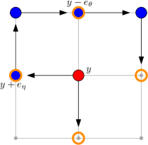
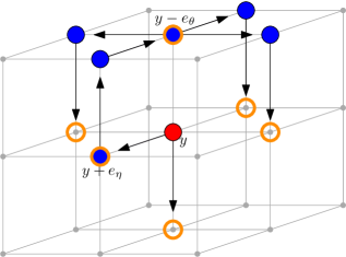
The goal of this section is to prove Theorem 3 To make the argument described in section 1.2 precise, we first need to define what we mean by a “cluster.” It turns out we only need to use a sort of directed cluster. Recall that $e_{\eta}$ and $e_{\theta}$ are distinct nearest neighbors of the origin with $e_{\eta}\neq-e_{\theta}$, and red sites satisfy a uniform ellipticity assumption that allows a walker to step from any red site $z$ to $z+e_{\theta}$ or $z+e_{\eta}$ with probability at least $\kappa$. Let $\mathcal{S}=\{e_{\eta}\}\cup\{-e_{\theta}\}\cup\{-e_{\theta}+e_{i}:1\leq i\leq 2d,e_{i}\neq\pm e_{\theta}\}$. If $d=3$ and $\theta=6$ so that $e_{\theta}$ is the “down” step , then $\mathcal{S}$ is the “cross” above the origin, along with one vertex that is horizontally adjacent to the origin. Now in a given environment $\omega$, define $C_{x}=C_{x}(\upsilon)$ to be the smallest subset of $\mathbb{Z}^{d}$ such that

• If $x$ is red, then $x\in C_{x}$;

• If $y\in C_{x}$ and $z\in y+\mathcal{S}$ is red, then $z\in C_{x}$.

Equivalently, $C_{x}$ is the set of all sites $y$ that are red and can be reached by a red path $\pi$ from $x$ to $y$ taking steps in $\mathcal{S}$; that is, a sequence $\pi=(x=\pi_{0},\pi_{1},\pi_{2},\ldots,\pi_{n}=y)$ of all red vertices such that for all $1\leq k\leq n$, $(\pi_{k}-\pi_{k-1})\in\mathcal{S}$. If $x$ is blue, then $C_{x}=\varnothing$.

Figure 3: The set $\mathcal{S}$ is depicted when $d=2$ on the left, and when $d=3$ on the right using an orthographic rendering. The origin is black, and vertices in $\mathcal{S}$ are purple.

The following proposition is the main ingredient in Theorem 3.

Proposition 1.

For all $\beta>0$, there exists $p^{*}\in(0,1)$ such that if $p>p^{*}$, then for all $x\in\mathbb{Z}^{d}$, for all $T\in\mathbb{N}$, and for every finite, nonempty set $C\subset\mathbb{Z}^{d}$, there exists $C^{\prime}\subset C$ with $|C^{\prime}|=|C|-1$ such that

$$\mathbb{E}^{0}[N_{x}^{T}\mathbbm{1}_{\{C_{x}=C\}}]\leq\beta^{-1}\mathbb{E}^{0}[N_{x}^{T}\mathbbm{1}_{\{C_{x}=C^{\prime}\}}]$$ (14)

Proof.

Fix $x\in\mathbb{Z}^{d}$ and $\beta>0$. Let $C\subset\mathbb{Z}^{d}$. We may freely assume that ${\bf P}(C_{x}=C)>0$, since otherwise (14) is trivial. In particular, $C_{x}$ is finite. Let $y$ be a vertex in $C$ maximizing $y\cdot(-e_{\theta})$, and of these (if there are more than one), let $y$ be a vertex maximizing $y\cdot e_{\eta}$. Let $C^{\prime}=C\setminus\{y\}$. We choose $y$ this way specifically to satisfy the following claim.

Claim 8.

If $C_{x}=C$, then every vertex in $y+\mathcal{S}$ is blue.

To see that this is true, assume $C_{x}=C$ and note that every vertex in $z\in y+\mathcal{S}$ has either $z\cdot(-e_{\theta})>y\cdot(-e_{\theta})$ or $z\cdot e_{\eta}>y\cdot e_{\eta}$, and therefore by the definition of $y$ cannot be in $C=C_{x}$. But since $y\in C_{x}$, the definition of $C_{x}$ says that any red vertex in $y+\mathcal{S}$ must also be in $C_{x}$. Therefore, all vertices in $y+\mathcal{S}$ are blue as claimed. We next claim

Now rather than considering directly the event $\{C_{x}=C^{\prime}\}$, we will consider a subset of this event. For a given pre-envirnoment $\upsilon$, define the pre-environment $\upsilon^{*}$ by

$$\upsilon^{*}(z)=\begin{cases}\upsilon(Z)\quad\quad\quad&\text{if }z\neq y\\ \text{red}&\text{if }z=y\end{cases}$$

Claim 9.

If $C_{x}(\upsilon^{*})=C$ and $y$ is blue, then $C_{x}(\upsilon)=C^{\prime}$.

This is because $y$ cannot be in $C_{x}(\upsilon^{\prime})$ as it is blue. However, if $z\in C_{x}(\upsilon^{\prime})$, then there is a red path from $x$ to $z$ taking steps in $\mathcal{S}$; by Claim 8, such a path cannot include $y$, so switching $y$ to blue cannot remove $z$ from $C_{x}$. On the other hand, switching any site to blue cannot create new red paths taking steps in $\mathcal{S}$, and therefore $C_{x}(\upsilon^{\prime})=C^{\prime}$, proving the claim.

Claim 10.

${\bf P}(C_{x}(\upsilon^{*})=C,~{}\upsilon(y)=\text{blue})=\frac{p}{1-p}{\bf P}(C_{x}=C)$.

To prove this claim, note that since $\upsilon^{*}$ is independent of $\upsilon(y)$,

$${\bf P}(C_{x}(\upsilon)=C)={\bf P}(C_{x}(\upsilon^{*})=C){\bf P}(y\text{ is red})=(1-p){\bf P}(C_{x}(\upsilon^{*})=C).$$ (15)

Similarly,

$${\bf P}(C_{x}(\upsilon^{*})=C,~{}\upsilon(y)=\text{blue})={\bf P}(C_{x}(\upsilon^{*})=C){\bf P}(y\text{ is blue})=p{\bf P}(C_{x}(\upsilon^{*})=C)$$ (16)

Combining (15) and (16) proves Claim 10.

Claim 11.

For a set $C\subset\mathbb{Z}^{d}$, Let $\partial C=(C+\mathcal{S})\setminus C$. Then for a set $C\subset\mathbb{Z}^{d}$ with ${\bf P}(C_{x}=C)>0$, the event that $\{C_{x}=C\}$ is precisely the event that every vertex in $C$ is red and every vertex in $\partial C$ is blue.

To prove this claim, note that ${\bf P}(C_{x}=C)>0$ if and only if $C$ is a finite set containing $x$ such that every $z\in C$ can be reached from $x$ by a path in $C$ taking only steps in $\mathcal{S}$. If every vertex in $C$ is red, this means every $z\in C$ can be reached from $x$ by a red path taking only steps in $\mathcal{S}$, so $C\subseteq C_{x}$. But if every vertex in $\partial C$ is blue, then $C$ satisfies the conditions in the definition of $C_{x}$. On the other hand, if $C_{x}=C$, it follows that every element of $C$ is red, and since any red vertex in $\partial C$ must also be in $C_{x}$, all vertices in $\partial C$ must be blue.

Now as in the proof of Claim 10, we let $\upsilon^{*}$ be the pre-environment that is equal to $\upsilon$ everywhere except possibly at $y$, where $\upsilon^{*}$ is red. Note that the event $\{C_{x}(\upsilon^{*})=C\}$ is the event that all vertices in $C^{\prime}$ are red in $\upsilon$, and all vertices in $\partial C$ are blue in $\upsilon$, with $y$ taking either color.

We wish to compare walks in three environments. In the first environment, we will have $C_{x}(\upsilon^{*})\neq C$. In the second, $C_{x}(\upsilon^{*})=C$ and $y$ is blue, so that $C_{x}(\upsilon)=C^{\prime}$. In the third, $C_{x}(\upsilon)=C_{x}(\upsilon^{*})=C$. We will couple the latter two walks with each other. The first only exists to allow us to create a tagged environment and walk drawn according to the annealed measure $\mathbb{P}^{0}$, and its dependence on the other two walks does not matter.

Consider, then, the measurable space given by the set

$$\text{\scalebox{1.5}{$\samech$}}=\Upsilon\times\Omega\times\mathcal{M}_{1}(\mathcal{N})^{C^{\prime}\cup\partial C}\times\mathcal{M}_{1}(\mathcal{N})^{2}\times[0,1]^{\mathbb{N}}\times[0,1]^{\mathbb{N}}\times\{1,2,3\}$$

endowed with Borel (product) sigma algebra, and the measure $\widehat{P}$ that is the product of ${\bf P}(\cdot|C_{x}(\upsilon^{*})\neq C)$ on $\Upsilon\times\Omega$, $\mu_{b}^{\partial C}\times\mu_{r}^{C^{\prime}}$ on $\mathcal{M}_{1}(\mathcal{N})^{C^{\prime}\cup\partial C}$, $\mu_{b}\times\mu_{r}$ on $\mathcal{M}_{1}(\mathcal{N})^{2}$, the Borel-Lebesgue product measure on $[0,1]^{\mathbb{N}}\times[0,1]^{\mathbb{N}}$, and on $\{1,2,3\}$ the discrete probability measure that selects $1$ with probability ${\bf P}(C_{x}(\upsilon^{*})\neq C)$, selects $2$ with probability ${\bf P}(C_{x}(\upsilon^{*})=C,~{}\upsilon(y)=\text{blue})$, and selects $3$ with probability ${\bf P}(C_{x}=C)$. Say a canonical element of this measure space is the 8-tuple

$$\shin=(\upsilon_{1},\omega_{1},\omega^{C^{\prime}\cup\partial C},\omega_{b}^{y},\omega_{r}^{y},{\bf U},{\bf V},A),$$

where $A\in\{1,2,3\}$.

Define $(\upsilon_{2},\omega_{2})$ to agree with $(\upsilon,\omega)$ everywhere except on $C\cup\partial C$, where $\upsilon_{2}$ is red on $C$ and blue on $\partial C$, and where $\omega_{2}^{C^{\prime}\cup\partial C}=\omega^{C^{\prime}\cup\partial C}$, and $\omega_{2}^{y}=\omega_{r}^{y}$. Define $(\upsilon_{3},\omega_{3})$ to agree with $(\upsilon_{2},\omega_{2})$ everywhere except at site $y$, where $\upsilon_{3}(y)=\text{red}$ and $\omega_{3}^{y}=\omega_{r}^{y}$. The probability space is constructed so that by Claim 11 and the i.i.d. property of environments, the law of $(\upsilon_{2},\omega_{2})$ is the law under ${\bf P}$ of a tagged environment $\boldsymbol{\omega}$ conditioned to have $C_{x}(\upsilon^{*})=C$ and $y$ blue, the law of $(\upsilon_{3},\omega_{3})$ is the law of a tagged environment conditioned to have $C_{x}=C$, and the law of $(\upsilon_{A},\omega_{A})$ is ${\bf P}$.

The following lemma is standard. We state it here for completeness and to make sure our coupling construction that depends on it is clear.

Lemma 3.

For all $a\in\mathbb{Z}^{d}$, there exists a map from $\phi:\Omega\times[0,1]^{\mathbb{N}}\to(\mathbb{Z}^{d})^{\mathbb{N}_{0}}$ taking a fixed environment $\omega$ and an infinite sequence ${\bf U}=(U_{n})_{n=1}^{\infty}$ and outputting a walk $\phi(\omega,{\bf U})=(X_{n})_{n=0}^{\infty}$, such that

1. For any fixed $\omega\in\Omega$, if ${\bf U}$ is a an i.i.d. sequence of uniform $(0,1)$ random variables, then $\phi(\omega,{\bf U})$ is drawn according to $P_{\omega}^{a}$.

2. If $\tau$ is a stopping time for $(X_{n})_{n=0}^{\infty}$, then on the event $\tau<\infty$, the regular conditional law of $(U_{n})_{n=\tau+1}^{\infty}$, conditioned on $(X_{n})_{n=0}^{\tau}$, is almost surely the i.i.d. uniform law.

Proof of Lemma 3.

Let $X_{0}=a$. For $k\geq 1$, if $X_{k-1}$ is defined, let

$$i_{k}=\min\left\{1\leq i\leq 2d:\sum_{j=1}^{i}\omega^{X_{k-1}}(e_{j})\leq U_{k}\right\},$$

and let $X_{k}=X_{k-1}+e_{i_{k}}$. This defines $X_{n}$ for all $n\geq 0$, and it is clear from the definition that (a) and (b) hold. ∎

We will define three coupled walks ${\bf X}^{1}=(X_{n}^{1})_{n=0}^{\infty}$, ${\bf X}^{2}=(X_{n}^{2})_{n=0}^{\infty}$ and ${\bf X}^{3}=(X_{n}^{3})_{n=0}^{\infty}$, drawn respectively according to $P_{\omega_{1}}^{0}$, $P_{\omega_{2}}^{0}$, and $P_{\omega_{3}}^{0}$. The only coupling that matters is between ${\bf X}^{2}$ and ${\bf X}^{3}$. The idea is that ${\bf X}^{3}$ steps with ${\bf X}^{2}$ until they hit site $y$ (the only site where transition probabilities in $\omega_{2}$ and $\omega_{3}$ can differ). After stepping away from $y$, the walk ${\bf X}^{2}$ “freezes,” while ${\bf X}^{3}$ continues to move independently until hitting the neighbor of $y$ where ${\bf X}^{2}$ is waiting. Once the two walks meet, they recouple and move together. Each time they hit $y$, they follow the same protocol. If it is ever the case that ${\bf X}^{3}$ never hits the neighbor of $y$ that ${\bf X}^{2}$ stepped to, then the two walks run forever independently (we do not think of ${\bf X}^{2}$ as being frozen in this case).

Let us formalize the above description. Let ${\bf X}^{1}$ be a walk started from the origin in environment $\omega_{1}$, using ${\bf U}$ to get its steps as in Lemma 3. Similarly, let ${\bf X}^{2}$ be a walk started from the origin in environment $\omega_{2}$, using ${\bf U}$ to get its steps. By Lemma 3, the law of ${\bf X}^{1}$, conditioned on $\omega_{1}$, is $P_{\omega_{1}}^{0}$, and similarly with ${\bf X}^{2}$. We will define ${\bf X}^{3}$ in terms of ${\bf X}^{2}$, $\omega_{3}$, and ${\bf V}$. Let $\tau_{1}:=\inf\{n\geq 0:X_{n}^{2}=y\}$ be the first hitting time of site $y$ by the walk ${\bf X}^{2}$, and recursively define $\tau_{k+1}:=\inf\{n\geq\tau_{k}:X_{n}^{2}=y\}$ as the time of the first return to $y$ after $\tau_{k}$. For $k$ such that $\tau_{k}<\infty$, define $y_{k}:=X_{\tau_{k}+1}^{2}$ to be the site ${\bf X}^{2}$ steps to after its $k$th visit to $y$.

Now if $\tau_{1}<\infty$, use the sequence ${\bf V}$ as in Lemma 3 to run a walk ${\bf Y}^{1}$ according to $P_{\omega_{3}}^{x}$ until time $b_{1}:=H_{y_{1}}$; that is, until the walk hits $y_{1}$, the location where ${\bf X}^{2}$ first stepped after hitting $y$. (Note that $b_{1}$ may be finite or infinite.) Now if $b_{1},\ldots,b_{k},\tau_{k+1}<\infty$, let $s_{k}:=\sum_{j=1}^{k}b_{k}$, and apply the function $\phi$ from Lemma 3 to the environment $\omega_{3}$ and $(V_{i})_{i=s_{k}+1}^{\infty}$ to run a walk ${\bf Y}^{k}$ until time $b_{k+1}:=H_{y_{k+1}}$, when the walk hits $y_{k+1}$.

Claim 12.

Let $\sigma({\bf V}^{c})$ be the sigma field generated by every entry of except ${\bf V}$ and A, and let $Q(\cdot)=\widehat{P}(\cdot|\sigma({\bf V}^{c}))$ be the law conditioned on $\sigma({\bf V}^{c})$. Then it is almost surely the case that under $Q$ on the event that $\tau_{1},\ldots,\tau_{k}<\infty$, the law of ${\bf Y}^{1}$ is the law under $P_{\omega_{3}}^{x}$ of a walk stopped at $H_{y_{1}}$, and for $j<k$, under the measure $Q$ conditioned on ${\bf Y}^{1},\ldots,{\bf Y}^{j}$ all being finite, the law of ${\bf Y}^{j+1}$ is the law under $P_{\omega_{3}}^{x}$ of a walk stopped at $H_{y_{j+1}}$ and ${\bf Y}^{1},\ldots,{\bf Y}^{j+1}$ are independent.

This claim follows from induction by repeated application of Lemma 3.

Now define ${\bf X}^{3}:=(X_{n}^{3})_{n=0}^{\infty}$ as the concatenation

$$(X_{n}^{2})_{n=0}^{\tau_{1}-1}~{}\frown~{}{\bf Y}^{1}~{}\frown~{}(X_{n}^{2})_{n=\tau_{1}+1}^{\tau_{2}-1}~{}\frown~{}{\bf Y}^{2}~{}\frown~{}(X_{n}^{2})_{n=\tau_{2}+1}^{\tau_{3}-1}~{}\frown~{}{\bf Y}^{3}~{}\frown~{}\cdots,$$ (17)

where $\frown$ denotes concatenation, and (17) is interpreted so that only terms that are defined are included. Note that our construction is such that with $\widehat{P}$-probability 1, if any sequence is defined, all previous sequences in the concatenation are defined and are finite, and conversely if the first $k$ sequences are finite, then the $(k+1)$st sequence is defined; this ensures that (17) almost surely gives us a single, well-defined infinite sequence.

Now let $\tilde{\boldsymbol{\omega}}=(\upsilon_{1},\omega_{1},\omega^{C^{\prime}\cup\partial C},\omega_{b}^{y},\omega_{r}^{y})$ (that is, the entries of that determine the three tagged environments, but not the walks).

Claim 13.

Conditioned on $\tilde{\boldsymbol{\omega}}$, each ${\bf X}^{i}$ is distributed according to $P_{\omega_{i}}^{0}$.

For $i=1,2$, this is immediate from Lemma 3. For $i=3$, it follows by induction with repeated application of the strong Markov property. Indeed, conditioned on the entries of $\tilde{\boldsymbol{\omega}}$, we know ${\bf X}^{2}$ follows $P_{\omega_{3}}^{0}$ until time $\tau_{1}$ , when the walk is at $y$ (since $\omega_{2}$ and $\omega_{3}$ agree except at $y$). Then ${\bf Y}^{1}$ follows the law of a walk in $\omega_{3}$ started at $y$, until it hits $y_{1}$. Then ${\bf X}^{2}$, started at time $\tau_{1}+1$, follows the law of a walk in $\omega_{3}$ started at $y_{1}$ until it hits $y$, and so on.

Claim 14.

The law of $(\boldsymbol{\omega}_{A},{\bf X}^{A})$ under $\widehat{P}$ is $\mathbb{P}^{0}$.

To prove the claim, let $E\subset\boldsymbol{\Omega}$ and $F\subset(\mathbb{Z}^{d})^{\mathbb{N}}$. Let $E_{1}=E\cap\{C_{x}(\upsilon^{*})\neq C\}$, $E_{2}=E\cap\{C_{x}(\upsilon^{*})=C,~{}\upsilon(y)=\text{blue}\}$, and $E_{3}=E\cap\{C_{x}(\upsilon)=C\}$. We have

$$\widehat{P}(\boldsymbol{\omega}_{A}\in E_{1},{\bf X}^{A}\in F) =\widehat{P}(A=1,\boldsymbol{\omega}_{1}\in E_{1},{\bf X}^{1}\in F)$$

$$={\bf P}(C_{x}(\upsilon^{*})\neq C)\widehat{P}(\omega_{1}\in E_{1},{\bf X}^{1}\in F)$$

$$={\bf P}(C_{x}(\upsilon^{*})\neq C)\int_{\{\boldsymbol{\omega}_{1}\in E_{1}\}}\widehat{P}({\bf X}^{1}\in F|\boldsymbol{\omega}_{1})d\widehat{P}(\boldsymbol{\omega}_{1}\in\cdot)$$

$$={\bf P}(C_{x}(\upsilon^{*})\neq C)\int_{\{\boldsymbol{\omega}_{1}\in E_{1}\}}P_{\omega_{1}}^{0}(F)d\widehat{P}(\boldsymbol{\omega}_{1}\in\cdot)$$

$$={\bf P}(C_{x}(\upsilon^{*})\neq C)\int_{E_{1}}P_{\omega}^{0}(F)d{\bf P}(\cdot|C_{x}(\upsilon^{*})\neq C)$$

$$=\int_{E_{1}}P_{\omega}^{0}(F)d{\bf P}$$

$$=\mathbb{P}^{0}(E_{1}\times F).$$

Similarly, $\widehat{P}(\boldsymbol{\omega}_{A}\in E_{2},{\bf X}^{A}\in F)=\mathbb{P}^{0}(E_{2}\times F)$ and $\widehat{P}(\boldsymbol{\omega}_{A}\in E_{3},{\bf X}^{A}\in F)=\mathbb{P}^{0}(E_{3}\times F)$. Adding these together, we get $\widehat{P}(\boldsymbol{\omega}_{A}\in E,{\bf X}^{A}\in F)=\mathbb{P}^{0}(E\times F)$, which proves the claim.

Now recall that $N_{x}^{T}=\sum_{n=0}^{T}\mathbbm{1}_{\{X_{n}=x\}}$ is the amount of time a walk spends at site $x$ up until time $T$. From Claim 14 and Claim 10 we may conclude

$$\mathbb{E}^{0}\left[N_{x}^{T}\mathbbm{1}_{\{C_{x}(\upsilon^{*})=C,~{}\upsilon(y)=\text{blue}\}}\right] =\widehat{E}\left[N_{x}^{T}({\bf X}^{A})\mathbbm{1}_{\{C_{x}(\upsilon_{A}^{*})=C,~{}\upsilon_{A}(y)=\text{blue}\}}\right]$$

$$=\widehat{E}[N_{x}^{T}({\bf X}^{2})\mathbbm{1}_{\{A=2\}}]$$ (18)

$$={\bf P}(C_{x}(\upsilon^{*})=C,~{}\upsilon(y)=\text{blue})\widehat{E}[N_{x}^{T}({\bf X}^{2})]$$ (19)

$$=\frac{p}{1-p}{\bf P}(C_{x}(\upsilon)=C)\widehat{E}[N_{x}^{T}({\bf X}^{2})],$$ (20)

and similarly,

$$\mathbb{E}^{0}\left[N_{x}^{T}\mathbbm{1}_{\{C_{x}(\upsilon^{*})=C,~{}\upsilon(y)=\text{blue}\}}\right]={\bf P}(C_{x}(\upsilon)=C)\widehat{E}[N_{x}^{T}({\bf X}^{3})].$$ (21)

Now examining (17), note that if $\tau_{k}>T$ for some $k$, then all steps in ${\bf X}^{3}$ corresponding to ${\bf Y}^{k}$ occur after time $T$. We thus have, with $\widehat{P}$-probability 1,

$$N_{x}^{T}({\bf X}^{3})\leq N_{x}^{T}({\bf X}^{2})+\sum_{k=1}^{T}\sum_{j=1}^{T}\sum_{i=1}^{2d}\mathbbm{1}_{\{\tau_{k}=j\}}\mathbbm{1}_{\{y_{k}=y+e_{i}\}}N_{x}^{T-j}({\bf Y}^{k}).$$ (22)

Now as in Claim 12, let $Q(\cdot)=\widehat{P}(\cdot|\sigma({\bf V}^{c}))$ be the law conditioned on $\sigma({\bf V}^{c})$, the sigma field generated by every entry of except ${\bf V}$. Taking expectations under $Q$ in (22), we almost surely get from Claim 12:

$$E_{Q}[N_{x}^{T}({\bf X}^{3})] \leq N_{x}^{T}({\bf X}^{2})+\sum_{k=1}^{T}\sum_{j=1}^{T}\sum_{i=1}^{2d}\mathbbm{1}_{\{\tau_{k}=j\}}\mathbbm{1}_{\{y_{k}=y+e_{i}\}}E_{Q}\left[N_{x}^{T-j}({\bf Y}^{k})\right].$$

$$=N_{x}^{T}({\bf X}^{2})+\sum_{k=1}^{T}\sum_{j=1}^{T}\sum_{i=1}^{2d}\mathbbm{1}_{\{\tau_{k}=j\}}\mathbbm{1}_{\{y_{k}=y+e_{i}\}}E_{\omega_{3}}^{y}\left[N_{x}^{(T-j)\wedge H_{y+e_{i}}}\right]$$

$$\leq N_{x}^{T}({\bf X}^{2})+\sum_{k=1}^{T}\sum_{j=1}^{T}\mathbbm{1}_{\{\tau_{k}=j\}}\max_{i=1,\ldots,2d}E_{\omega_{3}}^{y}\left[N_{x}^{(T-j)\wedge H_{y+e_{i}}}\right]$$ (23)

Claim 15.

For each $1\leq i\leq 2d$, we have

$$E_{\omega_{3}}^{y}\left[N_{x}^{(T-j)\wedge H_{y+e_{i}}}\right]\leq\max_{h=1,\ldots,2d}\frac{E_{\omega_{3}}^{y+e_{h}}\left[N_{x}^{(T-j-1)\wedge H_{y}}+\mathbbm{1}_{y=x}\right]}{\kappa^{5}}$$ (24)

To prove this claim, let $b=y+e_{i}$. For a walk ${\bf X}=(X_{n})_{n=0}^{\infty}$, define

$$T_{j}^{\prime}=T_{j}^{\prime}({\bf X}):=\inf\{n\geq T-j:y\notin\{X_{n-(T-j)+1},\ldots,X_{n-1},X_{n}\}\}$$

be the first time a walk has taken $T-j$ steps without hitting $y$. We imagine that a clock allows the walk to take $T-j$ steps, but the clock resets every time the walk hits $y$. The walk stops when the clock stops or when the walk hits $b$. The stopping time $T_{j}^{\prime}$ is useful because it allows us to use the strong Markov property every time the walk returns to $y$, but it is always at least $T-j$, so that we have

$$E_{\omega_{3}}^{y}\left[N_{x}^{(T-j)\wedge H_{b}}\right]\leq E_{\omega_{3}}^{y}\left[N_{x}^{T_{j}^{\prime}\wedge H_{b}}\right]$$ (25)

By conditioning and then using the strong Markov property and the definition of $T_{j}^{\prime}$, we can write

$$E_{\omega_{3}}^{y}\left[N_{x}^{T_{j}^{\prime}\wedge H_{b}}\right] =P_{\omega_{3}}^{y}(\tilde{H}_{y}>T_{j}^{\prime}\wedge H_{b})E_{\omega_{3}}^{y}\left[N_{x}^{T_{j}^{\prime}\wedge H_{b}}\hskip 3.0pt\vline\hskip 3.0pt\tilde{H}_{y}>T_{j}^{\prime}\wedge H_{b}\right]$$

$$\qquad\qquad+P_{\omega_{3}}^{y}(\tilde{H}_{y}<T_{j}^{\prime}\wedge H_{b})E_{\omega_{3}}^{y}\left[N_{x}^{T_{j}^{\prime}\wedge H_{b}}\hskip 3.0pt\vline\hskip 3.0pt\tilde{H}_{y}<T_{j}^{\prime}\wedge H_{b}\right]$$

$$=P_{\omega_{3}}^{y}(\tilde{H}_{y}>T_{j}^{\prime}\wedge H_{b})E_{\omega_{3}}^{y}\left[N_{x}^{T_{j}^{\prime}\wedge H_{b}}\hskip 3.0pt\vline\hskip 3.0pt\tilde{H}_{y}>T_{j}^{\prime}\wedge H_{b}\right]$$

$$\qquad\qquad+P_{\omega_{3}}^{y}(\tilde{H}_{y}<T_{j}^{\prime}\wedge H_{b})\left(E_{\omega_{3}}^{y}\left[N_{x}^{\tilde{H}_{y}-1}\hskip 3.0pt\vline\hskip 3.0pt\tilde{H}_{y}<T_{j}^{\prime}\wedge H_{b}\right]+E_{\omega_{3}}^{y}\left[N_{x}^{T_{j}^{\prime}\wedge H_{b}}\right]\right)$$

$$=E_{\omega_{3}}^{y}\left[N_{x}^{(T-j)\wedge H_{b}\wedge(\tilde{H}_{y}-1)}\right]+P_{\omega_{3}}^{y}(\tilde{H}_{y}<T_{j}^{\prime}\wedge H_{b})E_{\omega_{3}}^{y}\left[N_{x}^{T_{j}^{\prime}\wedge H_{b}}\right]$$

To justify the last equality, consider the time $(T-j)\wedge H_{b}\wedge(\tilde{H}_{y}-1)$. On the event $\{\tilde{H}_{y}>T_{j}^{\prime}\wedge H_{b}\}$, this time is the same as $T_{j}^{\prime}\wedge H_{b}$, while on the complementary event $\{\tilde{H}_{y}<T_{j}^{\prime}\wedge H_{b}\}$, it is the same as $\tilde{H}_{y}-1$. Solving for $E_{\omega_{3}}^{y}\left[N_{x}^{T^{\prime}\wedge H_{b}}\right]$ and noting that the complement of the event $\{\tilde{H}_{y}<T^{\prime}\wedge H_{b}\}$ can also be expressed as $\{\tilde{H}_{y}>(T-j)\wedge H_{b}\}$ gives us

$$E_{\omega_{3}}^{y}\left[N_{x}^{T^{\prime}\wedge H_{b}}\right]=\frac{E_{\omega_{3}}^{y}\left[N_{x}^{(T-j)\wedge H_{b}\wedge(\tilde{H}_{y}-1)}\right]}{P_{\omega_{3}}^{y}(\tilde{H}_{y}>(T-j)\wedge H_{b})}$$ (26)

Now $P^{y}(\tilde{H}_{y}>(T-j)\wedge H_{b})\geq P^{y}(H_{b}<\tilde{H}_{y})$. If $b=y+e_{\theta}$ or $b=y+e_{\eta}$, then $P^{y}(H_{b}<\tilde{H}_{y})\geq P^{y}(X_{1}=b)\geq\kappa$. If $b=y-e_{\theta}$, then $b$ can be reached by the path

$$(y+e_{\eta}~{},~{}y+e_{\eta}-e_{\theta}~{},~{}y-e_{\theta})$$

Any other neighbor of $y+e_{i}$ can be reached by the path,

$$(y~{},~{}y+e_{\eta}~{},~{}y+e_{\eta}-e_{\theta}~{},~{}y-e_{\theta},y-e_{\theta}+e_{i}~{},~{}y+e_{i}).$$

All sites in the above path, except for $y$ itself $y+e_{i}$, are in $y+\mathcal{S}$. Therefore, by are blue, and therefore the path can be taken with probability at least $\kappa^{5}$.

Figure 4: All nearest neighbors of $y$ (circled in orange) can be reached via paths of length no more than 5, where each step has probability at least $\kappa$ in $\omega_{3}$. The situations when $d=2$ and $d=3$ are depicted on the left and right, respectively.

With these considerations, (26) gives us

$$E_{\omega_{3}}^{y}\left[N_{x}^{T^{\prime}\wedge H_{b}}\right]\leq\frac{E_{\omega_{3}}^{y}\left[N_{x}^{(T-j)\wedge H_{b}\wedge(\tilde{H}_{y}-1)}\right]}{\kappa^{5}}.$$

Now by considering where the walk first steps after visiting site $y$ (and throwing away $H_{b}$), we can write

$$E_{\omega_{3}}^{y}\left[N_{x}^{T^{\prime}\wedge H_{b}}\right] \leq\max_{h=1,\ldots,2d}\frac{E_{\omega_{3}}^{y+e_{h}}\left[N_{x}^{(T-j-1)\wedge(H_{y}-1)}+\mathbbm{1}_{y=x}\right]}{\kappa^{5}},$$

which is (24). This proves the claim.

Now putting this into (23), we get

$$E_{Q}[N_{x}^{T}({\bf X}^{3})] \leq N_{x}^{T}({\bf X}^{2})+\sum_{k=1}^{T}\sum_{j=1}^{T}\mathbbm{1}_{\{\tau_{k}=j\}}\max_{h=1,\ldots,2d}\frac{E_{\omega_{3}}^{y+e_{h}}\left[N_{x}^{(T-j-1)\wedge(H_{y}-1)}+\mathbbm{1}_{y=x}\right]}{\kappa^{5}}$$

$$=N_{x}^{T}({\bf X}^{2})+\sum_{k=1}^{T}\sum_{j=1}^{T}\mathbbm{1}_{\{\tau_{k}=j\}}\max_{h=1,\ldots,2d}\frac{E_{\omega_{2}}^{y+e_{h}}\left[N_{x}^{(T-j-1)\wedge(H_{y}-1)}+\mathbbm{1}_{y=x}\right]}{\kappa^{5}}.$$ (27)

The equality comes from the fact that $\omega_{2}$ and $\omega_{3}$ agree away from site $y$. On the other hand, we can sort $N_{x}^{T}({\bf X}^{2})$ in terms of the visits of ${\bf X}^{2}$ to site $y$, throwing away any visits to $x$ before the first visit to $y$, to get

$$N_{x}^{T}({\bf X}^{2})\geq\sum_{k=1}^{T}\sum_{j=1}^{T}\mathbbm{1}_{\tau_{k}=j}\#\{j\leq n\leq T\wedge(\tau_{k+1}-1):X_{n}=x\}$$ (28)

Now recall that $\tilde{\boldsymbol{\omega}}$ is the information about the environments, but not the walks. Let $P_{\tilde{\boldsymbol{\omega}}}$ and $E_{\tilde{\boldsymbol{\omega}}}$ be respectively the probablity and expectation conditioned on $\tilde{\boldsymbol{\omega}}$. Taking expectations in (28) with respect to $P_{\tilde{\boldsymbol{\omega}}}$, we get (by Claim 13 and the strong Markov property):

$$E_{\tilde{\boldsymbol{\omega}}}[N_{x}^{T}({\bf X}^{2})]\geq\sum_{k=1}^{T}\sum_{j=1}^{T}P_{\tilde{\boldsymbol{\omega}}}(\tau_{k}=j)E_{\omega_{2}}^{y}[N_{x}^{(T-j)\wedge(H_{y}-1)}]$$ (29)

Now because $y$ is blue in $\omega_{2}$, the $P_{\omega_{2}}^{y}$, it has at least $\kappa$ of stepping to each of its neighbors, including the neighbor that maximizes $E_{\omega_{2}}^{y+e_{h}}[N_{x}^{(T-j-1)\wedge(H_{y}-1)}]$. By restricting to the event that the walk from $y$ steps to this site, we almost surely get

$$E_{\tilde{\boldsymbol{\omega}}}[N_{x}^{T}({\bf X}^{2})]\geq\sum_{k=1}^{T}\sum_{j=1}^{T}P_{\tilde{\boldsymbol{\omega}}}(\tau_{k}=j)\max_{h=1,\ldots,2d}\kappa E_{\omega_{2}}^{y+e_{h}}\left[N_{x}^{(T-j-1)\wedge(H_{y}-1)}+\mathbbm{1}_{y=x}\right].$$ (30)

Now because $\sigma(\tilde{\boldsymbol{\omega}})\subset\sigma({\bf V}^{c})$, we almost surely have $E_{\tilde{\boldsymbol{\omega}}}[E_{Q}[\cdot]]=E_{\tilde{\boldsymbol{\omega}}}[\cdot]$. Therefore, taking expectations in (27), we get

$$E_{\tilde{\boldsymbol{\omega}}}[N_{x}^{T}({\bf X}^{3})]\leq E_{\tilde{\boldsymbol{\omega}}}[N_{x}^{T}({\bf X}^{2})]+\sum_{k=1}^{T}\sum_{j=1}^{T}P_{\tilde{\boldsymbol{\omega}}}(\tau_{k}=j)\max_{h=1,\ldots,2d}\frac{E_{\omega_{2}}^{y+e_{h}}\left[N_{x}^{(T-j-1)\wedge(H_{y}-1)}+\mathbbm{1}_{y=x}\right]}{\kappa^{5}}.$$ (31)

Now combining (30) and (31) gives us

$$E_{\tilde{\boldsymbol{\omega}}}[N_{x}^{T}({\bf X}^{3})]\leq\left(1+\frac{1}{\kappa^{6}}\right)E_{\tilde{\boldsymbol{\omega}}}[N_{x}^{T}({\bf X}^{2})],~{}~{}a.s.$$ (32)

We now have everything we need to prove the lemma.

$$\mathbb{E}^{0}\left[N_{x}^{T}\mathbbm{1}_{\{C_{x}=C\}}\right] =\widehat{E}\left[N_{x}^{T}({\bf X}^{A})\mathbbm{1}_{\{C_{x}({\boldsymbol{\omega}_{A}})=C\}}\right]$$

$$=\widehat{E}\left[N_{x}^{T}({\bf X}^{3})\mathbbm{1}_{\{A=3\}}\right]$$

$$=\widehat{E}\left[N_{x}^{T}({\bf X}^{3})\right]{\bf P}(C_{x}=C)$$

$$=\widehat{E}\left[E_{\tilde{\boldsymbol{\omega}}}[N_{x}^{T}({\bf X}^{3})]\right]{\bf P}(C_{x}=C)$$ (33)

The first equality comes from Claim 14. The third comes from independence of $A$ from ${\bf X}^{3}$. Now by applying Claim 9, arguing as above, and then applying Claim 10, we get

$$\mathbb{E}^{0}\left[N_{x}^{T}\mathbbm{1}_{\{C_{x}=C^{\prime}\}}\right] \geq\mathbb{E}^{0}\left[N_{x}^{T}\mathbbm{1}_{\{C_{x}(\upsilon^{*})=C,~{}\upsilon(y)=\text{blue}\}}\right]$$

$$=\widehat{E}\left[E_{\tilde{\boldsymbol{\omega}}}[N_{x}^{T}({\bf X}^{2})]\right]{\bf P}(C_{x}(\upsilon^{*})=C,~{}\upsilon(y)=\text{blue})$$

$$=\widehat{E}\left[E_{\tilde{\boldsymbol{\omega}}}[N_{x}^{T}({\bf X}^{2})]\right]\frac{p}{1-p}{\bf P}(C_{x}=C)$$ (34)

Now (32), (33), and (34) combine to yield

$$\mathbb{E}^{0}[N_{x}^{T}\mathbbm{1}_{\{C_{x}=C\}}]\leq\frac{1-p}{p}\left(1+\frac{1}{\kappa^{6}}\right)\mathbb{E}^{0}[N_{x}^{T}\mathbbm{1}_{\{C_{x}=C^{\prime}\}}].$$ (35)

For any $\beta>0$ and fixed $\kappa$, we may choose $p^{*}$ close enough to 1 that for any $p>p^{*}$, $\frac{1-p}{p}\left(1+\frac{1}{\kappa^{6}}\right)\leq\beta^{-1}$, which proves the lemma. ∎

We are ready to prove our main theorem.

Proof of Theorem 3.

We are to show that for all $\varepsilon>0$, there exists $p^{*}<1$, depending only on $\varepsilon$, $d$, $v_{1}$, and $\kappa$, such that if $p>p^{*}$, then $\liminf_{n\to\infty}\frac{X_{n}\cdot\vec{u}}{n}\geq v_{1}-\varepsilon$, $\mathbb{P}^{0}$–almost surely.

Let $\varepsilon>0$. Choose $\beta=\frac{2\cdot 7^{d}}{\varepsilon}+7^{d}$. By Proposition 1 and Lemma 1, we may choose $p^{*}<1$ large enough that condition (C) is satisfied and for $p>p^{*}$, for all $x\in\mathbb{Z}^{d}$, $T\in\mathbb{N}$, and for every finite, nonempty set $C\subset\mathbb{Z}^{d}$, there exists $C^{\prime}\subset C$ with $|C^{\prime}|=|C|-1$ such that

$$\mathbb{E}^{0}\left[N_{x}^{T}\mathbbm{1}_{\{C_{x}=C^{\prime}\}}\right]\geq\beta\mathbb{E}^{0}\left[N_{x}^{T}\mathbbm{1}_{\{C_{x}=C\}}\right].$$

By induction, this implies that for every finite, nonempty set $C\subset\mathbb{Z}^{d}$,

$$\mathbb{E}^{0}\left[N_{x}^{T}\mathbbm{1}_{\{C_{x}=C\}}\right] \leq\beta^{-|C|}\mathbb{E}^{0}\left[N_{x}^{T}\mathbbm{1}_{\{C_{x}=\varnothing\}}\right]$$

$$=\beta^{-|C|}\mathbb{E}^{0}\left[N_{x}^{T}\mathbbm{1}_{\{x\text{ is blue}\}}\right].$$ (36)

Let $x\in\mathbb{Z}^{d}$. Note that $C_{x}$ is a lattice animal containing $x$. By [1, Equation 4.24], there are at most $7^{dk}$ such lattice animals of size $k$. Let $\mathcal{C}_{x}^{k}$ be the collection of all such lattice animals. We then have

$$\mathbb{E}^{0}[N_{x}^{T}\mathbbm{1}_{\{x\text{ is red}\}}] =\sum_{k=1}^{\infty}\sum_{C\in\mathcal{C}_{x}^{k}}\mathbb{E}^{0}[N_{x}^{T}\mathbbm{1}_{\{C_{x}=C\}}]$$ (37)

$$\leq\sum_{k=1}^{\infty}7^{dk}\beta^{-k}\mathbb{E}^{0}[N_{x}^{T}\mathbbm{1}_{\{x\text{ is blue}\}}]$$ (38)

$$=\mathbb{E}^{0}[N_{x}^{T}\mathbbm{1}_{\{x\text{ is blue}\}}]\sum_{k=1}^{\infty}\left(\frac{2}{\varepsilon}+1\right)^{-k}$$ (39)

$$=\frac{\varepsilon}{2}\mathbb{E}^{0}[N_{x}^{T}\mathbbm{1}_{\{x\text{ is blue}\}}].$$ (40)

Now (40) gives us (4) for $\alpha:=\frac{2v_{1}}{v_{2}\varepsilon}$. Now by Theorem 4, we have almost surely

$$\lim_{n\to\infty}\frac{X_{n}\cdot\vec{u}}{n} \geq\frac{(\alpha-1)v_{1}v_{2}}{v_{1}+\alpha v_{2}},$$

$$=\left(\frac{2}{2+\varepsilon}\right)\left(v_{1}-\frac{v_{2}\varepsilon}{2}\right)$$

$$\geq\left(1-\frac{\varepsilon}{2}\right)\left(v_{1}-\frac{\varepsilon}{2}\right)\geq v_{1}-\varepsilon.$$

∎

5 A strongly mixing counterexample

In this section, we show that the i.i.d. assumption in Theorem 3 is necessary by providing a counterexample to the statement—in fact, a counterexample to the statement of Theorem 2—with the i.i.d. assumption removed. For $\beta>0$ and $p\in(0,1)$, we will present an $\varepsilon>0$ and a measure ${\bf P}$ on environments where red and blue sites are as in Theorem 2, where every site is blue with probability at least $p$, and where $\lim_{n\to\infty}\frac{X_{n}\cdot e_{1}}{n}<\beta$.

Example 1.

Let $(U_{x})_{x\in\mathbb{Z}^{d}}$ be an i.i.d. collection of uniform $(0,1)$ random variables. Let $\delta>0$. For each $x=(a,b)\in\mathbb{Z}^{d}$, let $x^{*}$ be the closest vertex directly above $x$ whose associated uniform random variable is less than $\delta$. In other words, $x^{*}=(a,b^{*})$, where $b^{*}=\inf\{b^{\prime}\geq b:U_{(a,b^{\prime})}<\delta\}$. For each $x$, we have $U_{x^{*}}<\delta$ by definition. Let $x$ be red if in fact $U_{x^{*}}<\delta^{2}$. Otherwise, let $x$ be blue. Let ${\bf P}$ be the pushforward measure on environments.

Proposition 2.

Let $p\in(0,1)$ and $\beta>0$. For appropriately chosen $\varepsilon>0$ and $\delta>0$, the measure ${\bf P}$ described in Example 1 is such that sites are blue with probability at least $p$, and yet $\lim_{n\to\infty}\frac{X_{n}\cdot e_{1}}{n}<\beta$.

Proof.

We will defer our choice of $\delta$ to the end of the proof. For now, let $\varepsilon=\delta^{2}$. Note that for each $x\in\mathbb{Z}^{d}$, $x^{*}$ is independent of $U_{x^{*}}$, which is uniformly distributed on $(0,\delta)$. Now let $x_{*}$ be the nearest site directly below $x$ such that $U_{x_{*}}<\delta$. The distance from $x$ to $x^{*}$ and the distance from $x$ to $x_{*}$ are independent geometric random variables with parameter $\delta$. Hence there exists $C_{1}$ not depending on $\delta$ such that with probability at least $C_{1}$, $|x^{*}-x|$ and $|x-x_{*}|$ are both greater than $\frac{1}{\delta}$. With probability at least $C_{1}\delta$, then, $|x^{*}-x|$ and $|x-x_{*}|$ and $U_{x^{*}}<\delta^{2}$. On this event, all sites strictly between $x_{*}$ and $x^{*}$, as well as $x^{*}$, are red.

Now under the measure $\mathbb{P}^{0}$, for each $k\geq 1$ let $T_{k}=\inf\{n\in\mathbb{N}:X_{n}\cdot e_{1}\geq k\}$ be the $k$th time the walk enters a fresh half plane to the right of the origin. Let $\mathcal{F_{k}}$ be the sigma field generated by $(\omega^{x})_{x\cdot e_{1}<k}$ as well as $(X_{n})_{n=0}^{T_{k}}$. We consider $\mathbb{E}^{0}[T_{k+1}-T_{k}|\mathcal{F}_{k}]$.

Say $y=X_{T_{k}}$. Let $E_{k}$ be the event that $|y^{*}-y|,~{}|y-y_{*}|>\frac{1}{\delta}$ and $U_{y^{*}}<\delta^{2}$. By shift invariance and the fact that $E_{k}$ depends only on the environment to the right of sites that have been hit before time $T_{k}$, the event $E_{k}$ is independent of $\mathcal{F}_{k}$. On $E_{k}$, hitting the half-plane $\{x\cdot e_{1}\geq k+1\}$ requires the walk to either pass through a red site, which takes at least $O(\frac{1}{\delta^{2}})$ steps to happen, or to move around a wall of $\frac{1}{\delta}$ vertices in each direction. All vertical steps are up with probability $\frac{1}{4}$ and down with probability $\frac{1}{4}$, regardless of site color. Therefore, reaching a site with vertical position that differs from that of $y$ by $\frac{1}{\delta}$ or more takes of order $\frac{1}{\delta^{2}}$ steps. In fact, on the event $E_{k}$, with quenched probability at least $C_{2}$, it takes at more than $\frac{1}{\delta^{2}}$ steps to hit the half-plane $\{x\cdot e_{1}\geq k+1\}$. Therefore, with probability 1,

$$\mathbb{E}^{0}[T_{k+1}-T_{k}|\mathcal{F}_{k}]\geq C_{1}\delta C_{2}\frac{1}{\delta^{2}}=\frac{C_{1}C_{2}}{\delta}.$$

It follows that

$$\mathbb{E}^{0}[T_{k+1}-T_{k}]\geq C_{1}\delta C_{2}\frac{1}{\delta^{2}}=\frac{C_{1}C_{2}}{\delta},$$

whence it is standard to get

$$\lim_{n\to\infty}\frac{X_{n}\cdot e_{1}}{n}\leq\frac{\delta}{C_{1}C_{2}}$$

Now if we choose $\delta<\min(1-p,C_{1}C_{2}\beta)$, then sites blue with probability at least $p$, and $\lim_{n\to\infty}\frac{X_{n}\cdot e_{1}}{n}<\beta$. ∎

We now show that the measure ${\bf P}$ described in Example 1 has good mixing properties.

Proposition 3.

Under the measure ${\bf P}$ described in Example 1, the environment is $\psi$-mixing along vertical strips, and the vertical strips are i.i.d.

Proof.

That the vertical strips are i.i.d. follows immediately from the construction of ${\bf P}$. We now show that the environment is $\psi$-mixing along a vertical strip $\{(a,y):y\in\mathbb{Z}\}$. That the environment is strictly stationary along this strip follows, again, immediately from the construction. Now without loss of generality let $a=0$. Let $\mathcal{A}$ be the sigma field generated by $(\omega^{(a,y)})_{y\leq 0}$, and for $n\geq 1$, $\mathcal{B}_{n}$ be the sigma field generated by $(\omega^{(a,y)})_{y\geq n}$. Recall that $\psi$-mixing means

$$\lim_{n\to\infty}\sup_{\begin{subarray}{c}A\in\mathcal{A},~{}B\in\mathcal{B}_{n}\\ {\bf P}(A),{\bf P}(B)>0\end{subarray}}\left[\frac{{\bf P}(A\cap B)}{{\bf P}(A){\bf P}(B)}-1\right]=0$$ (41)

Let $P$ be the measure on the uniform variables used to determine $\omega$. By slight abuse of notation, if $E$ is an event in the sigma field on environments, we use $P(E)$ to denote the probability that the configuration of uniform random variables is such that $\omega\in E$. Using this convention, (41) is equivalent to the same equation with ${\bf P}$ replaced by $P$ throughout.

Now let $A\in\mathcal{A}$, and $B\in\mathcal{B}$, both with positive probability. Let $\mathcal{C}$ and $\mathcal{D}$ denote, respectively, the sigma fields generated by the uniform variables assigned to sites strictly below $(0,n)$ and above $(0,n)$, inclusive.

By construction, $B\in\mathcal{D}$. Let $M$ be the event that $0^{*}<n$. Equivalently, $M$ is the event that $U_{(}0,b)<\delta$ for some $b<n$. On the event $M$, the environment at and below $(0,0)$ is completely determined by the values of uniform random variables assigned to sites strictly below $(0,n)$. Therefore, $A\cap M\in\mathcal{C}$, so that $B$ is independent of $A\cap M$. Moreover, $A$ is independent of $M$, since the value of $U_{(}0,0^{*})$ is independent of $0^{*}$. We therefore have

$$P(A\cap M\cap B) =P(A\cap M)P(B)$$

$$=P(A)P(M)P(B)$$ (42)

so that

$$P(A\cap B) =P(A\cap B\cap M^{c})+P(A\cap M\cap B)$$

$$\geq P(A)P(B)P(M).$$ (43)

This gives us a lower bound on $P(A\cap B)$ in terms of $P(A)P(B)$. We now seek an upper bound. We have

$$P(A\cap B\cap M^{c}) =P(A\cap B\cap M^{c}\cap\{U_{n^{*}}<\delta^{2}\})+P(A\cap B\cap M^{c}\cap\{U_{n^{*}}>\delta^{2}\})$$ (44)

We examine the first term on the right side of (44). Note that on the event $M^{c}$, $0^{*}=n^{*}$, but $A$ depends on $\mathcal{D}$ only through $U_{(0,n^{*})}$, and in particular whether it is less than or greater than $\delta^{2}$. We therefore have

$$P(A\cap B\cap M^{c}\cap\{U_{n^{*}}<\delta^{2}\}) =P(M^{c}\cap\{U_{(0,n^{*})}<\delta^{2}\})P(A|M^{c}\cap\{U_{(0,n^{*})}<\delta^{2}\})P(B|U_{(0,n^{*})}<\delta^{2})$$

$$=P(M^{c})P(U_{(0,n^{*})}<\delta^{2})P(A|U_{(0,0^{*})}<\delta^{2})P(B|U_{(0,n^{*})}<\delta^{2})$$

On the other hand,

$$P(A\cap B\cap M\cap\{U_{n^{*}}<\delta^{2}\}) \geq P(M)P(U_{(0,0^{*})}<\delta^{2})P(U_{(0,n^{*})}<\delta^{2})P(A|U_{(0,0^{*})}<\delta^{2})P(B|U_{(0,n^{*})}<\delta^{2})$$

$$\geq\frac{\delta P(M)}{P(M^{c})}P(A\cap B\cap M^{c}\cap\{U_{n^{*}}<\delta^{2}\})$$

The same calculation can be done for the second term on the right side of (44). Putting these together, we have

$$P(A\cap B\cap M^{c})\leq\frac{P(M^{c})}{\delta P(M)}P(A\cap B\cap M)$$

Therefore,

$$P(A\cap B) =P(A\cap B\cap M^{c})+P(A\cap M\cap B)$$

$$\leq\left(\frac{P(M^{c})}{\delta P(M)}+1\right)P(A\cap B\cap M)$$ (45)

$$\overset{\eqref{eqn:1058}}{=}\left(\frac{P(M^{c})}{\delta P(M)}+1\right)P(A)P(B)P(M)$$

$$\overset{\eqref{eqn:1058}}{=}\left(\frac{P(M^{c})}{\delta}+P(M)\right)P(A)P(B).$$

Combining the above with (43), we get

$$P(M)\leq\frac{P(A\cap B)}{P(A)P(B)}\leq\left(\frac{P(M^{c})}{\delta}+P(M)\right)$$

Since $P(M)$ approaches 1 as $n\to\infty$, this completes the proof of the proposition. ∎

Remark.

We could also construct a counterexample to the statement of Theorem 3 without the i.i.d. assumption where the walk is not ballistic in direction $e_{1}$ at all. To do this, take a sequence of values of $\delta_{k}$ converging to 0, such that $\sum_{k}\delta_{k}<(1-p)$. Let a site $x$ be red if, for any $k\geq 1$, the nearest site $y$ above $x$ such that $U_{y}<\delta_{k}$ has in fact $U_{y}<\delta_{k}^{2}$. For red sites, set the probability of stepping in direction $e_{1}$ to 0, so that it is impossible to go “through” a wall. Moreover, the expected size of a new wall is infinite, so that the expected time to get around the wall is infinite, yielding zero speed. However, an environment constructed this way would not have mixing properties as good as the one in Example 1.

Question 1.

In Example 1, is the walk transient to the right? If so, can we improve the example to get a walk that is actually transient to the left?

6 Concluding Remarks and Further Questions

Theorem 3 shows that the asymptotic velocity of the walk in non-nestling models is stable under certain perturbations of the distribution on environments, including perturbations that break the non-nestling assumption. A desirable extension would be to prove a similar stability for a more general class of models.

Question 2.

Suppose we do not require $\mu_{b}$ to satisfy any sort of non-nestling assumption, but require only that if every site were distributed according to $\mu_{b}$, the walk would be transient in direction $\vec{u}$ with positive speed. In this setting, is something analogous to Theorem 3 still be true?

Our proof that the walk can be made to spend an arbitrarily small amount of time at red sites makes no use of the non-nestling assumption. However, a priori, the existence of the red sites could change which blue sites are visited, and in particular how often which types of blue sites are visited. Relaxing the non-nestling assumption would require translating our control on the frequency with which the walk visits red sites into a control on the extent to which the visits to red sites affects which blue sites are visited.

A related question is to test the limits of what perturbations are allowed.

Question 3.

Can we relax the uniform ellipticity assumption on $\mu_{r}$ even further?

Finally, we showed in Section 5 that the i.i.d. assumption—at least on the pre-environment—is necessary. But can we weaken the i.i.d. assumption at all?

Question 4.

Suppose we relax the i.i.d. assumption so that the pre-environment is i.i.d., but conditioned on the pre-environment, the transition probability vectors are not independent. Does Theorem 3 still hold?

References

- [1] G. Grimmett. Percolation. Die Grundlehren der mathematischen Wissenschaften in Einzeldarstellungen. Springer, 1999.
- [2] Olle Häggström and Johan Jonasson. Uniqueness and non-uniqueness in percolation theory. Probability Surveys, 3(none), jan 2006.
- [3] Steven A. Kalikow. Generalized random walk in a random environment. Ann. Probab., 9(5):753–768, 10 1981.
- [4] Christophe Sabot. Ballistic random walks in random environment at low disorder. The Annals of Probability, 32(4):2996 – 3023, 2004.
- [5] Daniel J. Slonim. Directional transience of random walks in dirichlet environments with bounded jumps. Preprint, submitted August 2021. https://arxiv.org/abs/2108.11424.
- [6] Fred Solomon. Random walks in a random environment. Ann. Probab., 3(1):1–31, 02 1975.
- [7] Alain-Sol Sznitman and Martin Zerner. A Law of Large Numbers for Random Walks in Random Environment. The Annals of Probability, 27(4):1851 – 1869, 1999.
- [8] O. Zeitouni. Random walks in random environment. In J. Picard, editor, Lecture notes in probability theory and statistics: École d’été de probabilités de Saint-Flour XXXI-2001, volume 1837 of Lect. Notes Math., pages 190–313. Springer, 2004.
- [9] Martin Zerner. A non-ballistic law of large numbers for random walks in i.i.d. random environment. Electron. Commun. Probab., 7:191–197, 2002.
- [10] Martin P. W. Zerner and Franz Merkl. A zero-one law for planar random walks in random environment. Ann. Probab., 29(4):1716–1732, 10 2001.
- [11] Martin P.W Zerner. Velocity and lyapounov exponents of some random walks in random environment. Annales de l’Institut Henri Poincare (B) Probability and Statistics, 36(6):737–748, 2000.