Ensemble models outperform single model uncertainties and predictions for operator-learning of hypersonic flows

Abstract

High-fidelity computational simulations and physical experiments of hypersonic flows are resource intensive. Training scientific machine learning (SciML) models on limited high-fidelity data offers one approach to rapidly predict behaviors for situations that have not been seen before. However, high-fidelity data is itself in limited quantity to validate all outputs of the SciML model in unexplored input space. As such, an uncertainty-aware SciML model is desired. The SciML model’s output uncertainties could then be used to assess the reliability and confidence of the model’s predictions. In this study, we extend a deep operator network (DeepONet) using three different uncertainty quantification mechanisms: mean-variance estimation (MVE), evidential uncertainty, and ensembling. The uncertainty aware DeepONet models are trained and evaluated on the hypersonic flow around a blunt cone object with data generated via computational fluid dynamics over a wide range of Mach numbers and altitudes. We find that ensembling outperforms the other two uncertainty models in terms of minimizing error and calibrating uncertainty in both interpolative and extrapolative regimes.

1 Introduction

Scientists and engineers gain understanding of large, complex systems like weather [1] and flight vehicles [2] by analyzing databases of how these systems behave, based on input parameters. These instances can be obtained via high-fidelity sources like computational simulation or physical experimentation. However, it is typically infeasible to obtain such data for every parameter configuration of interest. Further data can be generated by scientific machine learning (SciML) models that rapidly predict systems behavior for parameters not currently found in databases [3, 4, 5].

Because the high-fidelity ground truth is limited in quantity, it may not be sufficient to enable training of SciML models that can make predictions for the entire parameter space. This motivates the further incorporation of uncertainty quantification (UQ) into these SciML models [6, 7]. Uncertainties can be used to assess the reliability of predictions, and they can also be used to drive targeted acquisition of further data in an active learning loop [8, 9].

In this paper, we extend the deep operator network (DeepONet) [3] using three different UQ mechanisms: mean-variance estimation (MVE) [10], evidential uncertainty [11, 12, 13], and ensembling (Section 2.2). We evaluate these models on data generated by the steady-state compressible Navier-Stokes equations (NSE) with a non-uniform geometry based on a hypersonic flight vehicle (Appendix B) in both interpolation and extrapolation settings (Section 3). Although calibration in the extrapolation setting remains challenging to achieve, ensembling consistently outperforms other methods. This echoes findings in fields like chemistry [14] and motivates further development of probabilistic operator networks, especially those capable of extrapolating across parameter spaces.

Prior to the development of modern operator networks, UQ has been used in engineering fields to accelerate efficient data acquisition. Frequently, techniques like Gaussian process regression are used to predict a single target property like a drag coefficient, based on a small number of input parameters [2]. Here we consider the more general challenge of predicting pointwise uncertainties associated with a spatially-varying field like velocity. These pointwise uncertainties can still be aggregated into an acquisition function (e.g., [8]), or they can be analyzed in their own right (e.g., [15]).

2 Methods

2.1 Problem setup

We consider a general setting in which our training dataset $\mathcal{D}$ consists of measurement sets $(X,W^{d},\psi^{d}),d=1,\ldots,D$, where $X=\{x_{n}\}_{n=1}^{N}\subseteq\Omega\subseteq\mathbb{R}^{N_{x}}$ is a spatial mesh over a possibly-irregular geometry $\Omega$, shared across all measurement sets, $W^{d}=\{w^{d}_{n}\}_{n=1}^{N}\subseteq\mathbb{R}^{N_{w}}$ is a set of state variables values (with $w^{d}_{n}$ the value at mesh point $x^{d}_{n}$), and $\psi^{d}\in\mathbb{R}^{N_{\psi}}$ is a parameter vector. We learn a set of predictive models $\hat{w}_{\ell}$, one for each state variable $\ell=1,\ldots,N_{w}$.

In our setting (Appendix B), data satisfy a set of compressible NSE defined over a 3D axisymmetric geometry based on the Radio Attenuation Measurement (RAM)-C II flight vehicle [16, 17]. Due to the axisymmetry, there are two spatial degrees of freedom. The state variables are: $x$-velocity ($u_{1}$), $y$-velocity ($u_{2}$), density ($\rho$), and temperature ($T$). The parameter vector $\psi$ has two components: Mach number and altitude. Figure 1 demonstrates an example solution for this system.

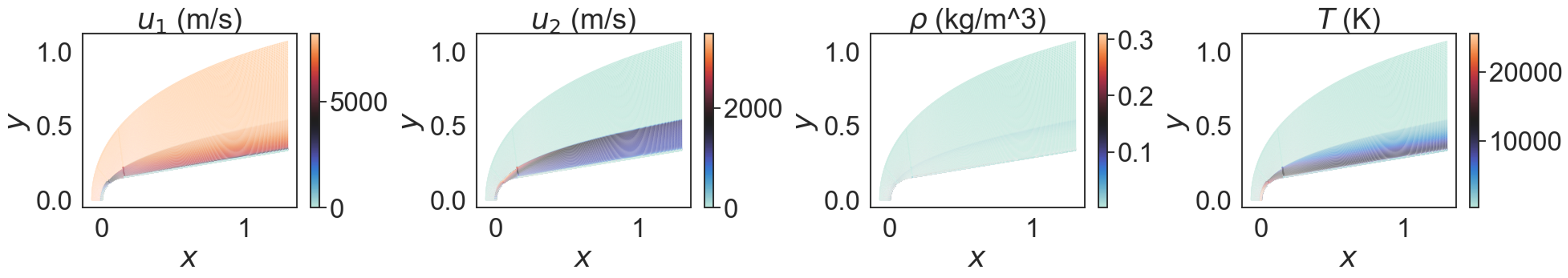
Figure 1: We show the four state variables that are solved for the axisymmetric geometry (Appendix B). This solution corresponds to Mach $25$ and altitude $46\text{\,}\mathrm{k}\mathrm{m}$.

2.2 Deep operator networks

To solve the RAM-C II fluid flow problem, we rely on the DeepONet [3] model. For a state variable $\ell$, the DeepONet $\hat{w}_{\ell}$ is a composition of multi-layer perceptrons (MLPs):

$$(x,\psi)\overset{\hat{w}_{\ell}}{\mapsto}f_{d}(f_{x}(x)\odot f_{\psi}(\psi)),$$ (1)

where $\odot$ is element-wise multiplication, $f_{x}$ is an encoder for the spatial points $x$, $f_{\psi}$ is an encoder for the parameters $\psi$, and $f_{d}$ is a decoder for the predicted state variable. MLPs have $\tanh$ activation functions. Each $\hat{w}_{\ell}^{\text{ONet}}$ is trained by using stochastic gradient descent (SGD) and Adam [18], over tuples $(x_{n},\psi^{d},w^{d}_{n})$ to minimize the squared errors $|w^{d}_{n,\ell}-\hat{w}_{\ell}^{\text{ONet}}(x_{n},\psi^{d})|^{2}$.

We extend the DeepONets with MVE [10], evidential [12], and ensemble [19] UQ methods. Each enables the DeepONets to output a mean $\mu_{\ell}$ and standard deviation $\sigma_{\ell}$, associated with a specified spatial point $x$ and parameter configuration $\psi$. Precise formulations for each UQ approach are standard, but we give them for reference in Appendix D.

3 Results

We evaluate models with respect to prediction error and uncertainty calibration for both in-domain (interpolating) and out-of-domain (OOD) (extrapolating) settings. Model error is measured with the relative error between a simulation’s predicted and ground truth state variables, measured in the normalized state variable space. We also compare the probabilistic DeepONets to a single (deterministic) DeepONet. Calibration is assessed using miscalibration area, as implemented in the Uncertainty Toolbox [20]. A higher miscalibration area means the model’s calibration is worse.

Our dataset (Appendix B) solves the system’s behavior across variation in the parameter vector $\psi=(\mathrm{Mach},\mathrm{altitude})$, where $\mathrm{Mach}\in\{10,11,\ldots,30\}$ and $\mathrm{altitude}\in\{20,22,\ldots,60\}$, in units of kilometers. This yields a total of $441$ simulations. We define the in-domain parameter regime as those simulations having parameters $\psi\in[12,28]\times[26,54]$ ($255$ simulations). The OOD parameter regime is subdivided into four regions: high Mach ($\psi\in\{29,30\}\times\{20,22,\ldots,60\}$), low Mach ($\psi\in\{10,11,12\}\times\{20,22,\ldots,60\}$), high altitude ($\psi\in\{10,11,\ldots,30\}\times\{56,58,60\}$, and low altitude ($\psi\in\{10,11,\ldots,30\}\times\{20,22,24\}$). For evaluating in-domain interpolation and comparing it to out-of-domain extrapolation, we sample $50$ simulations from the in-domain regime to use as a test set. All models use the same hyperparameters and training settings (Appendix C).

In Figure 2, we show that, in-domain, the ensemble model has the lowest errors for all state variables, with the deterministic model a close second. The MVE and evidential model have significantly higher errors across all state variables. Out-of-domain, all models perform more similarly, but on average, the ensemble model still has lower error. Turning to uncertainty calibration in-domain, the ensemble model has by far the best calibration (Figure 3). As training epochs increase, we observe that evidential model does not converge to meaningful uncertainty magnitudes. Out-of-domain, the ensemble model again has the best calibration of the three models.

None of the models have good calibration for $u_{1}$ when extrapolating. To understand why, we plot prediction error and uncertainty spatially (Figure 4), which reveals that uncertainty and error are spatially correlated. Regions of higher error and uncertainty are in regions in which $u_{1}$ changes rapidly over small spatial distances (i.e. at the hypersonic bow shock, in the boundary layer at the front tip of the cone, and at the surface boundary of the blunt cone). This implies that the DeepONet has difficulty fitting rapid spatial changes in state variables.

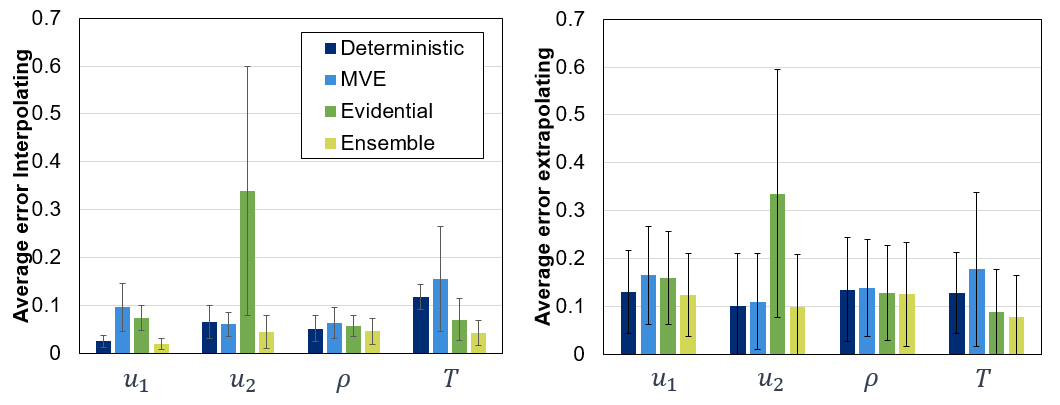
Figure 2: Average relative errors interpolating (in-domain) and extrapolating (OOD) for the four model types across state variables. When interpolating, the ensemble model has the lowest error, with the deterministic model a close second. When extrapolating, the four models perform more similarly, although on average, the ensemble model has the lowest error. For both interpolation and extrapolation, the MVE and evidential models have worse spread and error when predicting $T$ and $u_{2}$, respectively. The bars indicate average error across the domain’s test set for a given parameter. The error bars are the inter-quartile range of the errors across the domain’s test set. The ensemble model performs best when averaging over state variables in all domains, too (Table 1 in Appendix A).

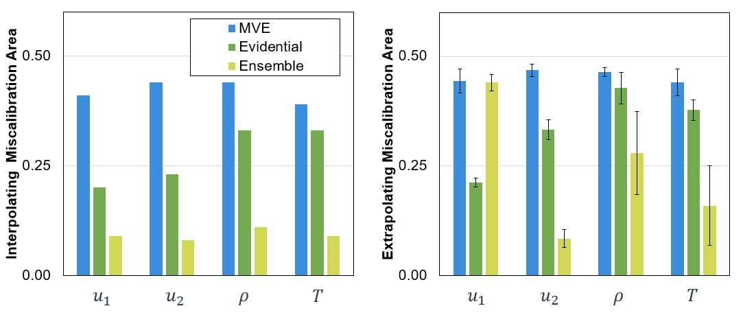
Figure 3: Uncertainty miscalibration areas interpolating (in-domain) and extrapolating (OOD) for the three probabilistic model types across state variables. When interpolating, the ensemble model has the lowest miscalibration area, which means that the uncertainties are well calibrated. The MVE and evidential models have significantly higher miscalbration areas. When extrapolating, the ensemble model has the lowest miscalibration area. No model has good uncertainty calibration when extrapolating for $u_{1}$. Interestingly, the evidential model has significantly lower miscalibration area than the MVE model for all state variables in-domain and for $u_{1}$ OOD than the other two models, implying that the evidential model has better uncertainty calibration. In fact, for some spatial points, the evidential model predicts large uncertainties of order $10^{4}$ for $u_{1}$ and $u_{2}$ and $10^{1}$ for $\rho$ and $T$ (Figure 5 in Appendix A), meaning that the evidential model is not converging on calibrated uncertainties. This is not captured by miscalibration area since it is insensitive to small numbers of outlier uncertainties. These uncertainties are far too large, as all state variables are normalized by mean and standard deviation of the train set before training, and thus, are all order ~1. The bars indicate the miscalibration area across the test domain. The error bars in extrapolation are the standard deviation of miscalibration area across the four extrapolation regimes (high Mach, high altitude, low Mach, low altitude).

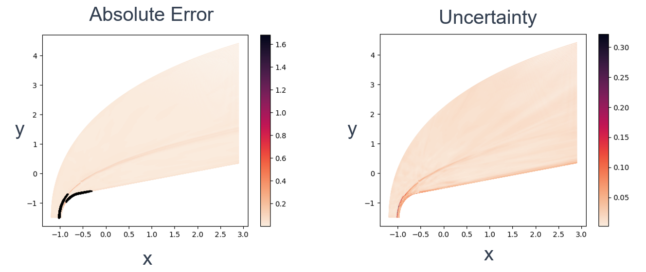
Figure 4: Spatial regions of higher uncertainty are correlated to regions of higher pointwise, absolute error in prediction for $u_{1}$. Darker points in both plots correspond to higher magnitudes of error and uncertainty. In the error plot, regions of relatively high error ($>0.5$) are highlighted in black. Higher error and uncertainty regions are concentrated where state variables rapidly change in value over short distances and at discontinuities (i.e. at the bow shock and at the surface boundary). This plot is from the in-domain test set, with Mach number $25$ and altitude $46\text{\,}\mathrm{k}\mathrm{m}$. Similar trends were observed across state variables and parameters.

4 Conclusion

We extend the DeepONet with three different UQ mechanisms: MVE, evidential uncertainty, and ensembling. We observe that the ensemble model outperforms both other UQ mechanisms in the in-domain (interpolative) and OOD (extrapolative) regimes for a case study on predicting $u_{1}$, $u_{2}$, $\rho$, and $T$ in the hypersonic flow around a blunt nose cone at various Mach numbers and altitudes. For the ensemble model, higher uncertainty is spatially correlated with higher error, which both tend to be concentrated in regions of large changes in state variable values over small distances. This motivates further research into the use of models that inherently account for nonlocal phenomena, such as neural basis functions (NBFs) [5], POD-DeepONets [21], and Fourier neural operators (FNOs) [4].

Appendix A Supplemental figures and tables

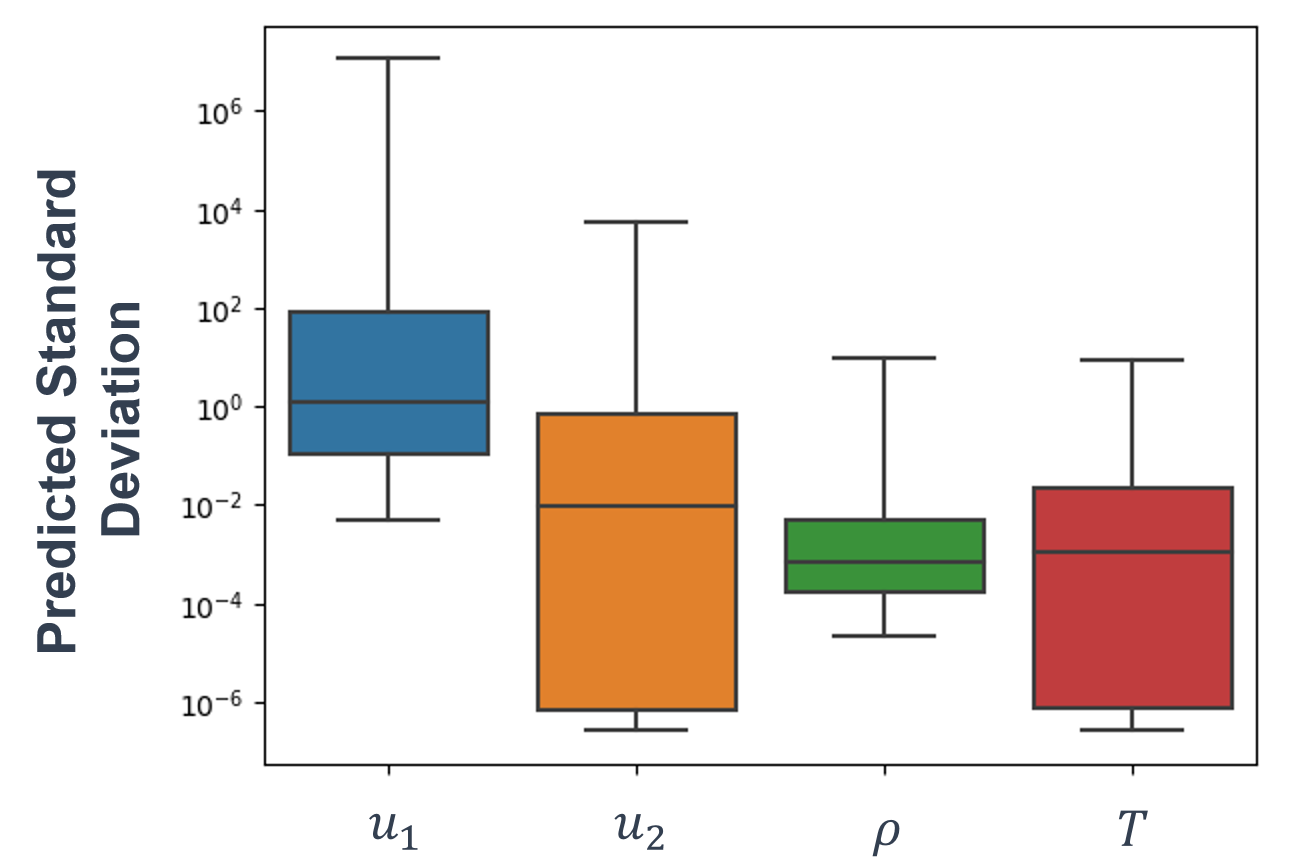
Figure 5: The evidential model does not converge on calibrated uncertainties. All data is normalized by mean and standard deviation, so predicted values are of magnitude ~1. The evidential model predicts uncertainties greater than $10^{4}$ (underconfident) for $u_{1}$ and $u_{2}$ and order $10^{1}$ for $\rho$ and $T$. This is not captured by miscalibration area since the metric is insensitive to small numbers of outlier uncertainties.

UQ mechanism	Evaluation domain	Mean Absolute Error	Calibration
Deterministic	In-domain	$0.0649\pm 0.0340$	n/a
	High Mach	$0.140\pm 0.0175$	n/a
	High Altitude	$0.0996\pm 0.0135$	n/a
	Low Mach	$0.130\pm 0.0174$	n/a
	Low Altitude	$0.124\pm 0.0356$	n/a
MVE	In-domain	$0.0939\pm.0378$	$0.42\pm 0.02$
	High Mach	$0.173\pm 0.0436$	$0.45\pm 0.03$
	High Altitude	$0.136\pm 0.0351$	$0.45\pm 0.00$
	Low Mach	$0.143\pm 0.0219$	$0.48\pm 0.01$
	Low Altitude	$0.139\pm 0.0367$	$0.44\pm 0.03$
Evidential	In-domain	$0.135\pm 0.118$	$0.27\pm 0.06$
	High Mach	$0.245\pm 0.200$	$0.32\pm 0.07$
	High Altitude	$0.158\pm 0.0871$	$0.35\pm 0.10$
	Low Mach	$0.141\pm 0.0253$	$0.35\pm 0.08$
	Low Altitude	$0.168\pm 0.0832$	$0.34\pm 0.08$
Ensembling	In-domain	$0.0378\pm 0.0105$	$0.09\pm 0.01$
	High Mach	$0.119\pm 0.0200$	$0.24\pm 0.14$
	High Altitude	$0.0846\pm 0.0185$	$0.22\pm 0.15$
	Low Mach	$0.118\pm 0.0213$	$0.27\pm 0.12$
	Low Altitude	$0.105\pm 0.0418$	$0.24\pm 0.18$

Table 1: We evaluate the four model types on in-domain and OOD prediction tasks in terms of accuracy and calibration. In contrast to Figure 2, which averages over all domains for each state variable, here we report mean absolute errors and standard deviations calculated over all points in each domain’s test set averaged over the four state variables. Consistent with Figure 2, we observe that ensembling has the lowest mean absolute errors for all evaluated models (in bold text) and, on average, the best calibration.

Appendix B Data generation

As training and evaluation data, we simulate high Mach number flow over a blunt nose cone, for a set of state variables governed by the compressible NSE. The geometry for our study is based on the second flight test from the RAM flight experiments performed in the 1960s: the RAM-C II vehicle [16, 17]. We represent the RAM-C II vehicle by an axisymmetric spherical blunt nose cone. The nose radius is $0.1524\text{\,}\mathrm{m}$ and connects tangentially to the cone body, which has a half-cone angle of $9\text{\,}{}^{\circ}$. The full body length of the configuration is $1.3\text{\,}\mathrm{m}$. We use CFD++ version 20.1 [22] to generate ground truth simulations.

Appendix C Network hyperparameters

Table 2 gives the hyperparameters used to train the DeepONets in this study. We do not find that evidential model performance varies significantly with evidential regularization hyperparameter $\lambda$ for values in the range $[10^{-3},1]$.

Hyperparameter	Value
# of hidden units for the spatial encoder $f_{x}$	$32$
# of layers for the spatial encoder $f_{x}$	$1$
# of hidden units for the parameter encode $f_{\psi}$	$32$
# of layers for the parameter encoder $f_{\psi}$	$1$
# of hidden units for the decoder $f_{d}$	$256$
# of layers for the decoder $f_{d}$	$3$
weight decay for training the DeepONets	$10^{-4}$
# epochs for training the DeepONets	$97$
evidential regularization strength $\lambda$	$10^{-2}$
# of ensemble members	$10$

Table 2: Hyperparameters for training the DeepONet models (Eq. 1)

Appendix D Uncertainty quantification for operator-learning

We evaluate three schemes for UQ in this work. MVE (Section D.1) and evidential uncertainty (Section D.2) are probabilistic methods that extend the network architecture and loss function, while ensembling (Section D.3) is not. Other techniques not considered here include dropout [23] and Gaussian mixture models (GMMs) [24].

D.1 Mean-variance estimation

In MVE, state variables are assumed to follow a conditionally normal distribution. The DeepONet $\hat{w}^{\ell}$ for the state variable $\ell$ has two output variables, the mean $\mu_{\ell}$ and variance $\sigma_{\ell}^{2}$:

$$(x,\psi) \overset{\hat{w}_{\ell}}{\mapsto} \mu_{\ell}(x,\psi),\sigma^{2}_{\ell}(x,\psi),$$ (2)

$$\mu_{\ell}(x,\psi) = [f_{d}(f_{x}(x)\odot f_{\psi}(\psi))]_{1}$$

$$\sigma^{2}_{\ell}(x,\psi) = \mathrm{SoftPlus}[f_{d}(f_{x}(x)\odot f_{\psi}(\psi))]_{2},$$

where the $\mathrm{SoftPlus}$ ensures nonnegativity of variance. MVE DeepONets are trained by minimizing the Gaussian negative log-likelihood (NLL):

$$\mathrm{Loss}((x,\psi),w_{\ell})=\log\sigma_{\ell}^{2}(x,\psi)+\frac{(\mu_{\ell}(x,\psi)-w_{\ell})^{2}}{\sigma_{\ell}^{2}(x,\psi)},$$ (3)

for a partial data point $((x,\psi),w_{\ell})\in\mathbb{R}^{N_{x}}\times\mathbb{R}^{N_{\psi}}\times\mathbb{R}$.

D.2 Evidential uncertainty

In evidential uncertainty [11, 12, 13], a normal inverse-gamma (NIG) probabilistic model is imposed on the data:

$$w_{\ell}|x,\psi \sim \mathcal{N}(\mu_{\ell},\sigma^{2}_{\ell})$$ (4)

$$\mu_{\ell}|x,\psi \sim \mathcal{N}(\gamma_{\ell},\sigma^{2}_{\ell}/v_{\ell})$$

$$\sigma^{2}_{\ell}|x,\psi \sim \Gamma^{-1}(\alpha_{\ell},\beta_{\ell}).$$

From this hierarchical model, we have the predicted state variable value as $\mathbb{E}[\mu_{\ell}]=\gamma_{\ell}$, the predicted aleatoric uncertainty as $\mathbb{E}[\sigma^{2}_{\ell}]=\beta_{\ell}/(\alpha_{\ell}-1)$, and the predicted epistemic uncertainty as $\mathrm{Var}[w_{\ell}]=\beta_{\ell}/(v_{\ell}(\alpha_{\ell}-1))$. Thus, the predictive model $\hat{w}_{\ell}$ for state variable $\ell$ is given by:

$$x,\psi \overset{\hat{w}_{\ell}}{\mapsto} \gamma_{\ell},v_{\ell},\alpha_{\ell},\beta_{\ell}$$ (5)

$$\gamma_{\ell} = [f_{d}(f_{x}(x)\odot f_{\psi}(\psi))]_{1}$$

$$v_{\ell} = \mathrm{SoftPlus}[f_{d}(f_{x}(x)\odot f_{\psi}(\psi))]_{2}$$

$$\alpha_{\ell} = \mathrm{SoftPlus}[f_{d}(f_{x}(x)\odot f_{\psi}(\psi))]_{3}+1$$

$$\beta_{\ell} = \mathrm{SoftPlus}[f_{d}(f_{x}(x)\odot f_{\psi}(\psi))]_{4},$$

where each $f_{\ell}$ is a neural network (NN).

For a partial datapoint $((x,\psi),w_{\ell})\in\mathbb{R}^{N_{X}}\times\mathbb{R}^{N_{W}}\times\mathbb{R}$, the evidential loss function [12] is:

$$\mathrm{Loss}((x,\psi),w) = \sum_{\ell}\mathrm{Loss}^{NLL}((x,\psi),w_{\ell})+\lambda\,\mathrm{Loss}^{R}((x,\psi),w_{\ell}),$$ (6)

where $\mathrm{Loss}^{NLL}$ is a NLL:

$$\mathrm{Loss}^{NLL}((x,\psi),w_{\ell}) = \frac{1}{2}\log\frac{\pi}{v_{\ell}}-\alpha_{\ell}\log\Omega_{\ell}+\log\frac{\Gamma(\alpha_{\ell})}{\Gamma(\alpha_{\ell}+(1/2))}$$ (7)

$$+\left(\alpha_{\ell}+\frac{1}{2}\right)\log\left((w_{\ell}-\gamma_{\ell}^{2}v_{\ell}+\Omega_{\ell}\right)$$

$$\Omega_{\ell} = 2\beta_{\ell}(1+v_{\ell})$$

and $\mathrm{Loss}^{R}$ is a regularization term:

$$\mathrm{Loss}^{R}((x,\psi),w_{\ell}) = |w_{\ell}-\gamma_{\ell}|(2v_{\ell}+\alpha_{\ell})$$ (8)

D.3 Ensembling

In ensembling [19], a set of $B$ models $\hat{w}_{\ell,1},\ldots,\hat{w}_{\ell,B}$ are independently trained from different network weight initializations. Then the predicted means and standard deviations are $\mu_{\ell}(x,\psi)=\underset{b}{\mathrm{mean}}\{\hat{w}_{\ell,b}\}$ and $\sigma_{\ell}(x,\psi)=\underset{b}{\mathrm{StdDev}}\{\hat{w}_{\ell,b}\}$.

References

- [1] Jordan G. Powers, Joseph B. Klemp, William C. Skamarock, Christopher A. Davis, Jimy Dudhia, David O. Gill, Janice L. Coen, David J. Gochis, Ravan Ahmadov, Steven E. Peckham, Georg A. Grell, John Michalakes, Samuel Trahan, Stanley G. Benjamin, Curtis R. Alexander, Geoffrey J. Dimego, Wei Wang, Craig S. Schwartz, Glen S. Romine, Zhiquan Liu, Chris Snyder, Fei Chen, Michael J. Barlage, Wei Yu, and Michael G. Duda. The weather research and forecasting model: Overview, system efforts, and future directions. Bulletin of the American Meteorological Society, 98(8):1717 – 1737, 2017.
- [2] Kevin R. Quinlan, Jagadeesh Movva, Elizabeth V. Stein, and Ana Kupresanin. Leveraging Multi-Fidelity Aerodynamic Databasing to Efficiently Represent a Hypersonic Design Space. 2021.
- [3] Lu Lu, Pengzhan Jin, Guofei Pang, Zhongqiang Zhang, and George Em Karniadakis. Learning nonlinear operators via deeponet based on the universal approximation theorem of operators. Nature Machine Intelligence, 3(3):218–229, Mar 2021.
- [4] Zongyi Li, Nikola Borislavov Kovachki, Kamyar Azizzadenesheli, Burigede liu, Kaushik Bhattacharya, Andrew Stuart, and Anima Anandkumar. Fourier neural operator for parametric partial differential equations. In International Conference on Learning Representations, 2021.
- [5] David Witman, Alexander New, Hicham Alkandry, and Honest Mrema. Neural basis functions for accelerating solutions to high mach euler equations. In ICML 2022 2nd AI for Science Workshop, 2022.
- [6] Dongkun Zhang, Lu Lu, Ling Guo, and George Em Karniadakis. Quantifying total uncertainty in physics-informed neural networks for solving forward and inverse stochastic problems. Journal of Computational Physics, 397:108850, 2019.
- [7] Yibo Yang, Georgios Kissas, and Paris Perdikaris. Scalable uncertainty quantification for deep operator networks using randomized priors. Computer Methods in Applied Mechanics and Engineering, 399:115399, 2022.
- [8] Christopher J. Arthurs and Andrew P. King. Active training of physics-informed neural networks to aggregate and interpolate parametric solutions to the navier-stokes equations. Journal of Computational Physics, 438:110364, 2021.
- [9] Shibo Li, Zheng Wang, Robert Kirby, and Shandian Zhe. Deep multi-fidelity active learning of high-dimensional outputs. In Gustau Camps-Valls, Francisco J. R. Ruiz, and Isabel Valera, editors, Proceedings of The 25th International Conference on Artificial Intelligence and Statistics, volume 151 of Proceedings of Machine Learning Research, pages 1694–1711. PMLR, 28–30 Mar 2022.
- [10] D.A. Nix and A.S. Weigend. Estimating the mean and variance of the target probability distribution. In Proceedings of 1994 IEEE International Conference on Neural Networks (ICNN’94), volume 1, pages 55–60 vol.1, 1994.
- [11] Murat Sensoy, Lance Kaplan, and Melih Kandemir. Evidential deep learning to quantify classification uncertainty. In Proceedings of the 32nd International Conference on Neural Information Processing Systems, NIPS’18, page 3183–3193, Red Hook, NY, USA, 2018. Curran Associates Inc.
- [12] Alexander Amini, Wilko Schwarting, Ava Soleimany, and Daniela Rus. Deep evidential regression. In Proceedings of the 34th International Conference on Neural Information Processing Systems, NIPS’20, Red Hook, NY, USA, 2020. Curran Associates Inc.
- [13] Ava P. Soleimany, Alexander Amini, Samuel Goldman, Daniela Rus, Sangeeta N. Bhatia, and Connor W. Coley. Evidential deep learning for guided molecular property prediction and discovery. ACS Central Science, 7(8):1356–1367, 2021.
- [14] Aik Rui Tan, Shingo Urata, Samuel Goldman, Johannes C. B. Dietschreit, and Rafael Gómez-Bombarelli. Single-model uncertainty quantification in neural network potentials does not consistently outperform model ensembles, 2023.
- [15] Arnaud Vadeboncoeur, Ieva Kazlauskaite, Yanni Papandreou, Fehmi Cirak, Mark Girolami, and Omer Deniz Akyildiz. Random grid neural processes for parametric partial differential equations. In Andreas Krause, Emma Brunskill, Kyunghyun Cho, Barbara Engelhardt, Sivan Sabato, and Jonathan Scarlett, editors, Proceedings of the 40th International Conference on Machine Learning, volume 202 of Proceedings of Machine Learning Research, pages 34759–34778. PMLR, 23–29 Jul 2023.
- [16] Erin Farbar, Iain D. Boyd, and Alexandre Martin. Numerical prediction of hypersonic flowfields including effects of electron translational nonequilibrium. Journal of Thermophysics and Heat Transfer, 27(4):593–606, 2013.
- [17] Pawel Sawicki, Ross S. Chaudhry, and Iain D. Boyd. Influence of chemical kinetics models on plasma generation in hypersonic flight. In AIAA Scitech 2021 Forum, 2021.
- [18] Diederik P. Kingma and Jimmy Ba. Adam: A Method for Stochastic Optimization, 2014. doi:10.48550/ARXIV.1412.6980.
- [19] Balaji Lakshminarayanan, Alexander Pritzel, and Charles Blundell. Simple and scalable predictive uncertainty estimation using deep ensembles. In Proceedings of the 31st International Conference on Neural Information Processing Systems, NIPS’17, page 6405–6416, Red Hook, NY, USA, 2017. Curran Associates Inc.
- [20] Youngseog Chung, Ian Char, Han Guo, Jeff Schneider, and Willie Neiswanger. Uncertainty toolbox: an open-source library for assessing, visualizing, and improving uncertainty quantification. arXiv preprint arXiv:2109.10254, 2021.
- [21] Lu Lu, Xuhui Meng, Shengze Cai, Zhiping Mao, Somdatta Goswami, Zhongqiang Zhang, and George Em Karniadakis. A comprehensive and fair comparison of two neural operators (with practical extensions) based on fair data. Computer Methods in Applied Mechanics and Engineering, 393:114778, 2022.
- [22] MultiMedia LLC. CFD++, Version 20.1, 2023.
- [23] Yarin Gal and Zoubin Ghahramani. Dropout as a bayesian approximation: Representing model uncertainty in deep learning. In Proceedings of the 33rd International Conference on International Conference on Machine Learning - Volume 48, ICML’16, page 1050–1059. JMLR.org, 2016.
- [24] Albert Zhu, Simon Batzner, Albert Musaelian, and Boris Kozinsky. Fast uncertainty estimates in deep learning interatomic potentials. The Journal of Chemical Physics, 158(16):164111, 04 2023.