Diversity and Diffusion:
Observations on Synthetic Image Distributions with Stable Diffusion

Abstract

Recent progress in text-to-image (TTI) systems, such as Stable Diffusion, Imagen, and DALL-E 2, have made it possible to create realistic images with simple text prompts. It is tempting to use these systems to eliminate the manual task of obtaining natural images for training a new machine learning classifier. However, in all of the experiments performed to date, classifiers trained solely with synthetic images perform poorly at inference, despite the images used for training appearing realistic. Examining this apparent incongruity in detail gives insight into the limitations of the underlying image generation processes. Through the lens of diversity in image creation vs. accuracy of what is created, we dissect the differences in semantic mismatches in what is modeled in synthetic vs. natural images. This will elucidate the roles of the image-language model, CLIP, and the image generation model, diffusion. We find four issues that limit the usefulness of TTI systems for this task: ambiguity, adherence to prompt, lack of diversity, and inability to represent the underlying concept. We further present surprising insights into the geometry of CLIP embeddings.

1 Introduction

Large text-to-image (TTI) models have visually demonstrated the remarkable recent progress in AI, enabling high-quality synthesis of images from textual prompts. The most commonly used successful models employ diffusion, a gradual denoising process (Ho, Jain, and Abbeel 2020). These diffusion-based generative text-to-image models (Saharia et al. 2022; Rombach et al. 2021; Chang et al. 2023; Yu et al. 2022; Ramesh et al. 2022; Nichol et al. 2022) have seen impressive improvements in quality that rival or exceed modern Generative Adversarial Networks (GAN) techniques (Kang et al. 2023; Dhariwal and Nichol 2021).

As generative models continue to produce increasingly realistic images, beyond creating images for artistic or more general human viewing, we can ask whether synthetic images can replace traditional datasets gathered by hand. To an untrained eye, the images often appear to be suitable; see Figure 1. If so, creating datasets, even ones much larger than today’s datasets, can become a far less manual process. Conceivably, it is possible that the generative models could produce even more diverse images than the distribution of a hand-gathered set, potentially exceeding their utility.

Multiple works have explored exactly this avenue and have trained classifiers with synthetic-only image sets, typically using ImageNet-1K (Deng et al. 2009) classification as a benchmark (Azizi et al. 2023; Sariyildiz et al. 2023; Bansal and Grover 2023). Interestingly, none of these studies, using purely synthetic images, matches, or even comes close, to the accuracy of training with natural images. Instead, they combine synthetic and natural images to improve accuracy. Nonetheless, even then, a too large proportion of synthetic images degrades the performance; the number of natural images required increases with the number of synthetic images, only increasing the manual process.

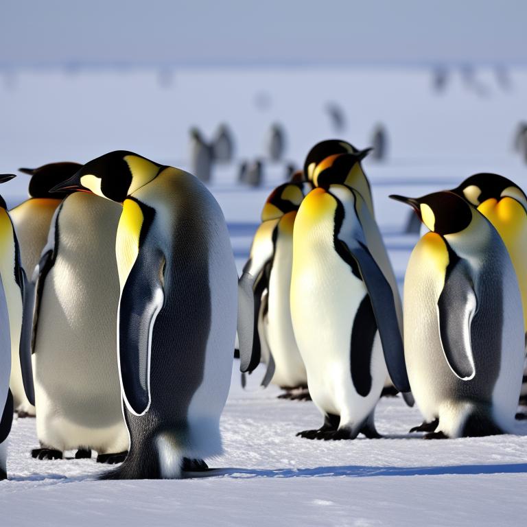
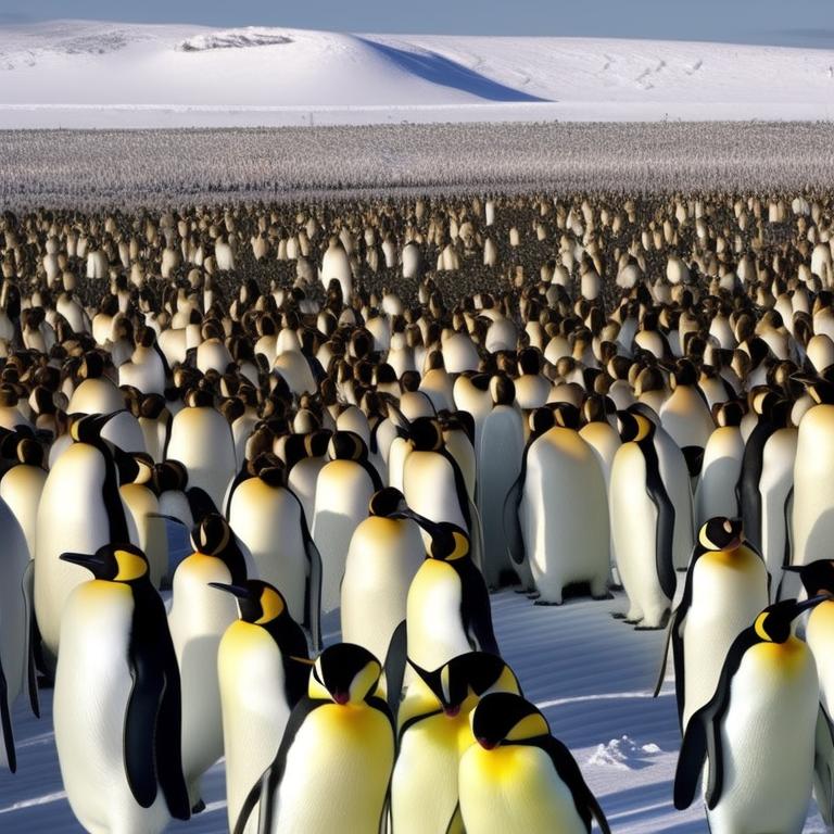
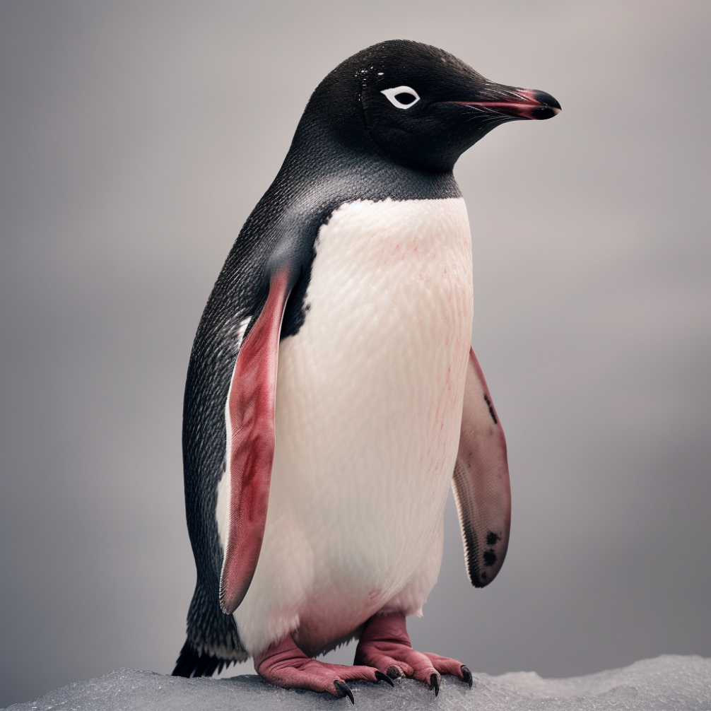
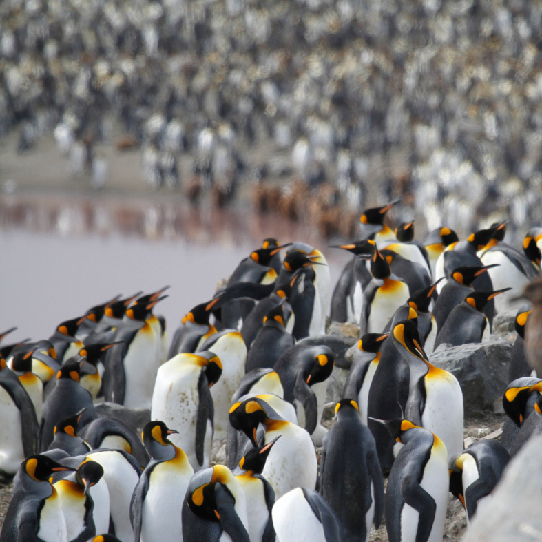
Figure 1: Penguins. Top Row: Synthetic Images. Bottom Row: Natural photographs from  (iNaturalist 2023).

Our primary contribution is to uncover the root causes of the poor performance with purely synthetic images. Given the nascent nature of this field, even choosing which aspects to study is open for discussion. Here, we examine the roles of diversity and meaning-shift in both the internal representations and the generation procedures used inside a TTI system. To make our work as widely applicable as possible, we study Stable Diffusion’s synthesized images in comparison to ImageNet’s natural images.

We present related work in Section 2. Section 3 gives four reasons for the drop in accuracy using synthetic images. Section 4 examines the geometry of prompt and image embeddings created by CLIP. Finally, recognizing that zero-shot classifiers are equivalent to k-nn classifiers with class centroids, we look at k-nn classifiers broadly.

2 Closely Related Work

Synthetic Images for Classification. Foundational to our study are recent attempts at ImageNet classification training using synthetic images. Using the short names for ImageNet-1K classes, or prompts derived from them, a TTI system, such as Stable Diffusion, is used to generate thousands of images for that class that are then used for training. While the ImageNet set has approximately 1,000 images per class, synthetic sets are not limited to this. All of the previous studies used techniques to improve the synthetic image prompts that led to accuracy improvements over pure short-names. Though some studies could exceed their natural-image-only benchmark on subsets of ImageNet, we constrain our study to Top-1 accuracy on the full ImageNet validation set. For the full test, all of the studies see a very large gap (often more than 30%) between training on a natural images and synthetic ones (Sariyildiz et al. 2023; Azizi et al. 2023; Xie et al. 2016). As a middle ground, they all explore forms of fine-tuning or data augmentation for natural images to improve baseline accuracies. However, this technique still demonstrates a continued reliance on hand-gathered data.

Diffusion Models. Many generative TTI systems use diffusion (Ho, Jain, and Abbeel 2020; Song, Meng, and Ermon 2021), including Stable Diffusion (SD), Imagen, DALL-E 2 (Ramesh et al. 2022), Openjourney (PromptHero 2023), Versatile Diffusion (Xu et al. 2023) and Glide (Nichol et al. 2022). Diffusion has been used in other generative domains such as audio synthesis (Kong et al. 2021) and video (Chen et al. 2023). Our analysis investigates the contribution of diffusion to accuracy; however, the ideas trivially generalize to non-diffusion TTI systems like Cogview (Ding et al. 2021), Parti (Yu et al. 2022) and Muse (Chang et al. 2023). Additionally, we note that methods of fine-tuning diffusion, such as Dreambooth and textual inversion (Ruiz et al. 2023; Gal et al. 2022; Tewel et al. 2023) can be used to better create images similar to ImageNet classes. This yields improvements, but again requires the use of an existing image database.

Synthetic Data from GANs. Like diffusion-based-TTI, Generative Adversarial Networks (GANs) (Goodfellow et al. 2020) can create synthetic training examples without hand-implemented domain knowledge, for example for facial expression classification (Bhattarai et al. 2020), traffic sign classification (Dewi et al. 2021) and semantic segmentation (Sankaranarayanan et al. 2018). Such synthetic data for training are typically labeled in the tasks domain while the diffusion models are largely classifier-free. For the wider task of broad text-based synthesis, TTI systems have often shown more fidelity to natural images (Yu et al. 2022).

3 The Pitfalls of Purely Synthetic Data

Synthetic images are poor replacements for natural images when training classifiers. We offer four explanations for this.

Reason #1: Prompt and Class Ambiguity

Many short names (Athalye 2020) for the ImageNet-1K classes can be inadequate for use with a TTI system. First, the ImageNet short names are often less precise than their associated WordNet (Miller 1995) synset description. For example, the synset “African chameleon, Chamaeleo chamaeleon” is more precise than the ImageNet short name, “chameleon.” In contrast to some previous studies, we avoid these issues by starting with synset descriptions as prompts.

Second, often the words in the synset may have homonyms and are therefore ambiguous. SD may have a different meanings than the synset descriptions; it is biased to produce likely images, where “likely” is influenced by popular culture. Figure 2 shows the query “drake” for which ImageNet contains ducks but SD produces the homonymous performer.

“drake”			“whiskey jug”
ImageNet	SD		ImageNet	SD

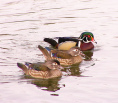
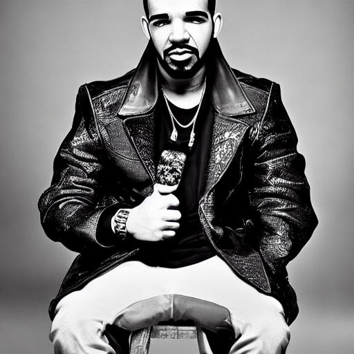
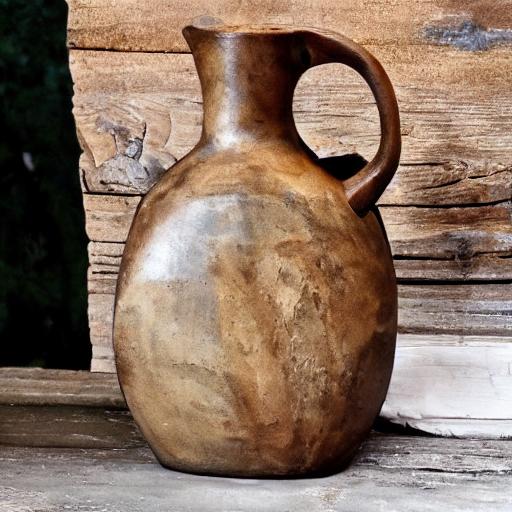
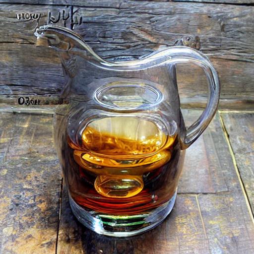
Figure 2: Images from ImageNet and generated by SD. “drake” confuses the duck with the homonymous performer. “whiskey jug” shows the bias in ImageNet.

Third, synsets are often repetitive, e.g. the “chameleon” class (above), causing SD to produce multiple instances of the object rather than interpreting these as synonyms.

Fourth, when humans gather datasets, biases may be introduced in data collection. When ImageNet is used for both training and evaluation without visual examination, these biases remain hidden because train/evaluation are consistent with each other. However, when compared with the common usage of the label, the biases become evident. For example, ImageNet’s “whiskey jug” images are clay jars with distinctive labels, a subset of the general class of "whiskey jugs." See Figure 2. TTI systems will not be limited to a specific type of whiskey jar and will produce out-of-domain images relative to ImageNet. See (Beyer et al. 2020; Stock and Cisse 2018; Tsipras et al. 2020) for a discussion of ImageNet’s limitations. Unfortunately, this has often not been addressed in recent work, and may substantially impact the results.

We broadly categorize these problems as ambiguity. To alleviate these issues, we generated 50 images for each label and classified them with a ResNet-RS-152 classifier. We manually reviewed the 300 labels with the lowest accuracy. For classes with low accuracy that we determined to be caused solely by ambiguity, the labels were minimally clarified. This resulted in 105 modifications.

Before continuing to the deeper analysis of synthetic images, we quantify the improvement of the modified prompts. In our baseline synthetic image set, for each of the 1000 classes we created 1200 training images and 50 evaluation images (total 1,250,000 images created) using Stable Diffusion v1.5 (SD) with the original synsets as prompts. We term this set Synset. Next, we replaced the 105 classes with images created using the newly clarified prompts (131,250 images replaced); this disambiguated set is Disamb.

We use these two sets, each with training and evaluation splits, as drop-in replacements for the original ImageNet set; see Table 1. In our first test, when the standard ImageNet trained network is tested on the Synset and Disamb sets, the performance drops to 68.5% and 72.2% respectively (lines 2-3). This is the first indication that (1) there is a mismatch in the images between ImageNet and the synthetic images, and (2) the modification to the 105 classes was beneficial.

	Training Set	Evaluation Set	Accuracy(%)
1.	Imagenet	Imagenet	80.8
2.	Imagenet	Synset	68.5
3.	Imagenet	Disamb	72.2
4.	Synset	Imagenet	23.0
5.	Synset	Synset	98.5
6.	Disamb	Imagenet	26.3
7.	Disamb	Disamb	98.8

Table 1: Accuracy of various train and evaluation sets, measured by training a ResNet-RS-152.

In our second test, we use the Synset and Disamb sets for training. Training with Synset and evaluating on ImageNet precipitously reduces performance to 23% (random is .1%) (line 4). Training with Disamb improves the results modestly to 26.3%. What happened? Given that training with natural images and evaluating with synthesized images did not suffer as much degradation as training with synthesized and evaluating with natural images, perhaps the synthesized images have less diversity. The useful synthetic images may represent less breadth. Table 1 lines 5 & 7 support this line of inquiry: if we both train and evaluate with synthetic images only, and they have low diversity, the accuracies should be high. They are: 98-99%. This leads to Reasons #3 & #4, which will contrast diversity with centroid-shift, in which a different concept may be represented in the images than expected. Next, reason #2 continues with the role of the prompt and controlling its effect on image generation.

Reason #2: Adherence to the Text Prompt

In most TTI systems, there is an explicit parameter that controls how much the generated image should be conditioned on the given textual prompt. In SD, the parameter clip_guidance_scale (cgs) controls the influence of the prompt on the otherwise unconditional image generation. The default in SD is $cgs=7.5$, which was used for generating both Synset and Disamb sets. We hypothesized that this factor, which represents the adherence to the prompt, may be too high to allow enough diversity in synthetic images.

At $cgs=1.0$, images have no added compliance to the prompt but should be relatively “likely” with respect to SD’s training set. In practice, however, the synthetic images appear largely incoherent. Empirically, the coherence seems to be more consistent when $cgs\geq 2.5$. Lower values produce images that are less compliant to the prompt, but lack of coherence makes them unsuitable for use in training. In contrast, at $cgs=7.5$, images appear very well lit, highly saturated, and more professionally composed. Interestingly, this also makes them poor candidates for training as the ImageNet validation set does not appear professional or unnaturally saturated. Figure 3 shows examples. For completeness, we trained using $cgs=1.0$ images (1,250,000 images created) and results were substantially lower than those in Table 1&2.

	1.0	2.5	5.0	7.5
		(Disamb2.5)		(Disamb)
grand piano, piano
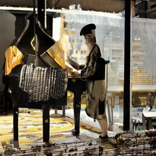
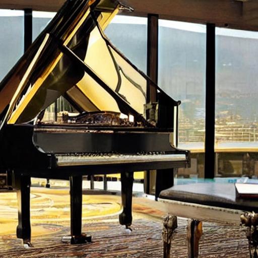
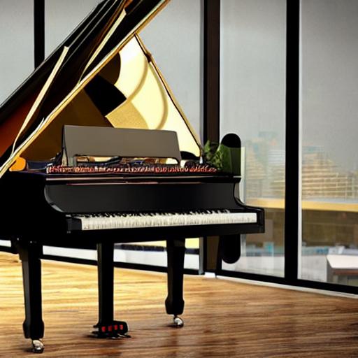
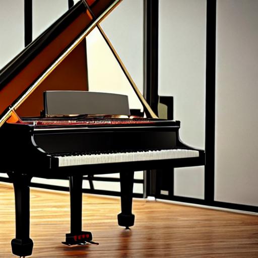
pickup, pickup truck
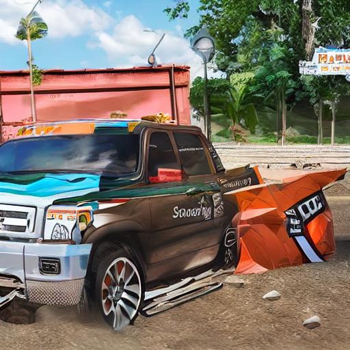
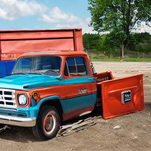
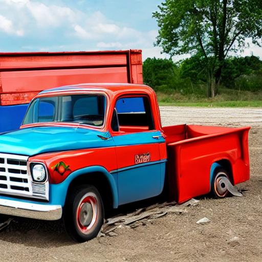
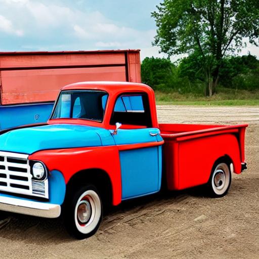
burrito
green mamba

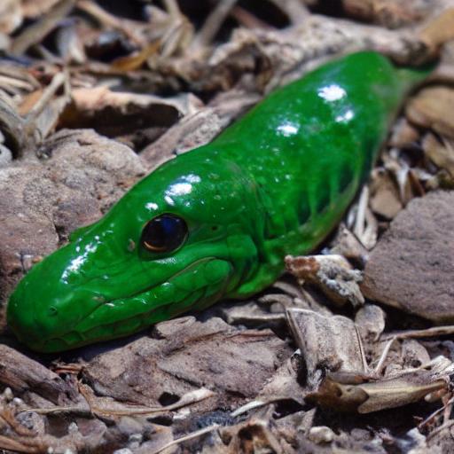
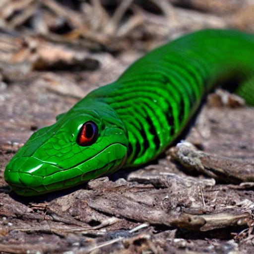
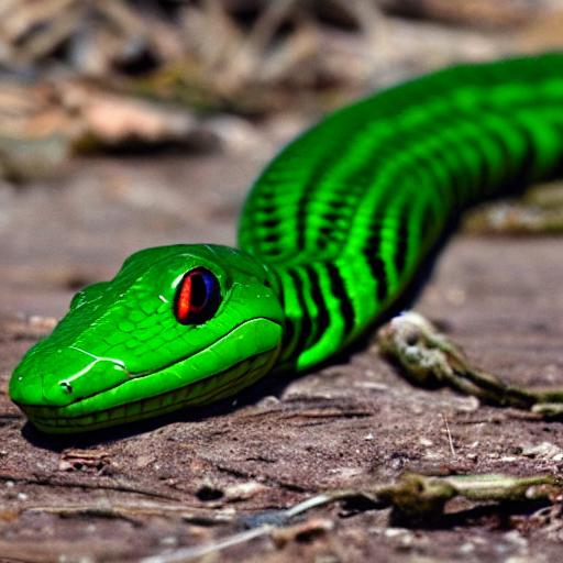
Figure 3: Images for various clip_guidance_scale ($cgs$) values. At $cgs=1.0$, the images are of low quality. With $cgs$ set to higher values, the image sets lose diversity.

Consequently, we created a new set, Disamb2.5, that uses the same prompts as Disamb, but uses ${cgs=2.5}$ (1,250,000 images created). This significantly improved the performance, as shown in Table 2.

	Training Set	Evaluation Set	Accuracy(%)
1.	ImageNet	Disamb2.5	59.2
2.	ImageNet	PromptAug	50.9
3.	Disamb2.5	ImageNet	43.4
4.	Disamb2.5	Disamb2.5	91.0
5.	PromptAug	ImageNet	45.3
6.	PromptAug	PromptAug	81.2

Table 2: Accuracy of various train and evaluation sets, measured by training a ResNet-RS-152.

The Disamb2.5 result in Table 2-line 3, indicates that a wider variety of ImageNet validation images are correctly classified when trained with this new dataset. Compared to the previous setting of $cgs=7.5$ for Disamb, this is a raw improvement of 17%. A byproduct of the increased diversity is that the synthetic images are more difficult for a standard, natural-image-trained network to classify (Table 2, line 1 vs. Table 1, line 3). With more diversity, the training and evaluation with Disamb2.5 (line 4) is harder than with Disamb $cgs=7.5$.

Next, rather than relying on SD to implicitly introduce diversity through reducing prompt adherence, we can also explicitly encourage diversity through prompt augmentation. Similarly, (Radford et al. 2021) uses labels prefixed with “a photo of a”, while (Pratt, Liu, and Farhadi 2022) used prompts created with GPT-3. Our next set, PromptAug, creates a unique prompt for each image – even within a class. For this, we used a combinatorial set of {pre+post}-fix prompt modifiers, and for each class selected 1,250. See Figure 4.

 Creation process for the PromptAug Set  

$looks$  $\overset{{\scriptscriptstyle\operatorname{R}}}{\leftarrow}$ [beautiful, ugly, ..]
$extent_{1,2}$  $\overset{{\scriptscriptstyle\operatorname{R}}}{\leftarrow}$ [slightly, very, …]
$typical$  $\overset{{\scriptscriptstyle\operatorname{R}}}{\leftarrow}$ [uncommon, typical, …]
$size$  $\overset{{\scriptscriptstyle\operatorname{R}}}{\leftarrow}$ [small, large, …]
$location$  $\overset{{\scriptscriptstyle\operatorname{R}}}{\leftarrow}$ [partially_occluded, centered, …]
$style$  $\overset{{\scriptscriptstyle\operatorname{R}}}{\leftarrow}$ [overexposed, hyper_sharp_image, …]

prompt $\leftarrow$ $looks+(extent_{1}*typical)+(extent_{2}*size)+\newline \hskip 39.74872pt\mathbf{class\_name}+location+style$

Figure 4: In PromptAug, each image is generated with a unique prompt. 2 sample values shown for each modifier.  $\overset{{\scriptscriptstyle\operatorname{R}}}{\leftarrow}$ randomly selects a single element from a set. The full set is available to download. Samples are in Appendix B.

Each modifier takes on a single, randomly chosen, value from its small set. The modifiers are broadly applicable and can be used with any class label. No adjectives describing color, texture, or feel were used as they inevitably would be inappropriate for some objects. As can be seen in Table 2, using the images of this set yields a small improvement in accuracy (line 5 vs. line 3). Again, if we look at the indicators of greater diversity in these synthetic images, when ImageNet-trained networks are used for classification, the accuracy drops (Table 2, line 2 vs. line 1). When PromptAug images are used for both training and evaluation, accuracy is again reduced in comparison to previous experiments (line 6 vs. line 4). Figure 5 presents synthesized images in each set.

	Synset		Disamb	Disamb2.5	PromptAug
jay		a bird of type jay
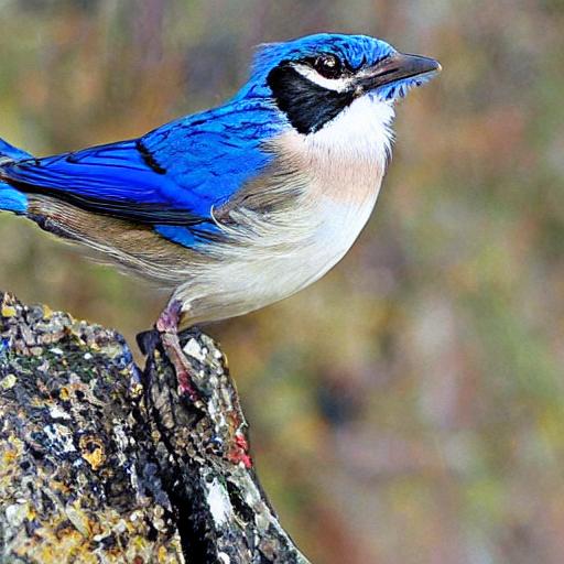
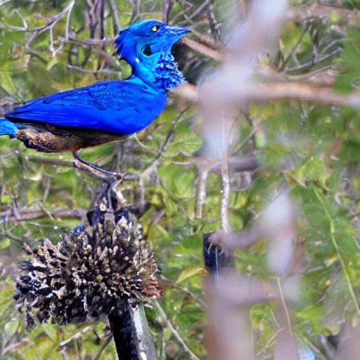
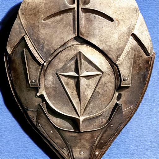
breastplate aegis,egis		breastplate
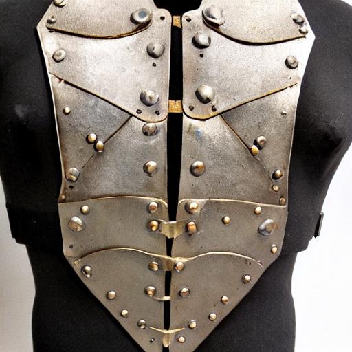
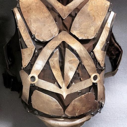
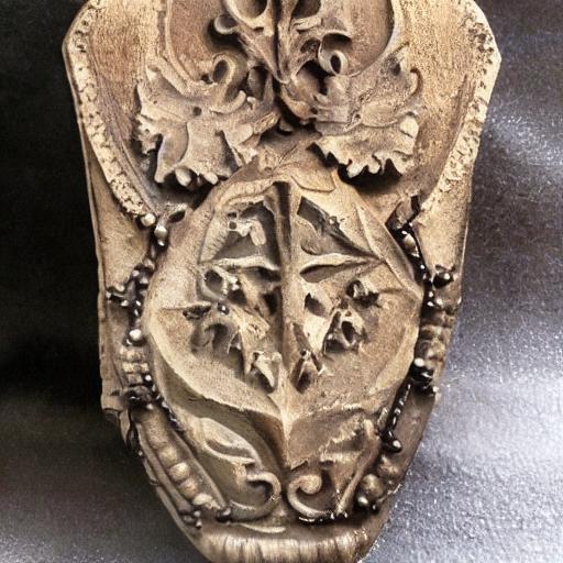
mortar		mortar and pestle
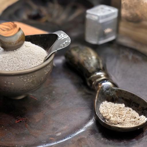
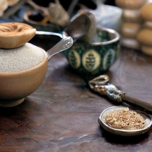
crane		a crane bird
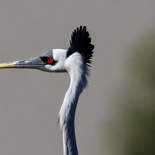
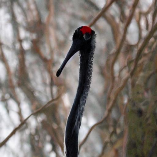
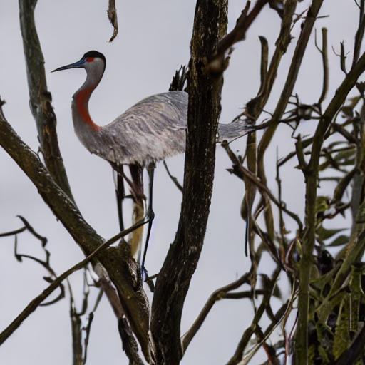
Centroid
Distance	n/a		$1.23{\times}10^{-5}$	$2.05{\times}10^{-5}$	$2.49{\times}10^{-5}$

Figure 5: Four classes, their prompts, and an image from each class, all using the same initial diffusion noise (e.g. same seed). All four classes were in the set of 105 prompts modified for Disamb. The Centroid Distance increases substantially with each set (n/a for Synset as the prompts are ambiguous). PromptAug prompts are created by the procedure in Figure 4 using the shown class names.

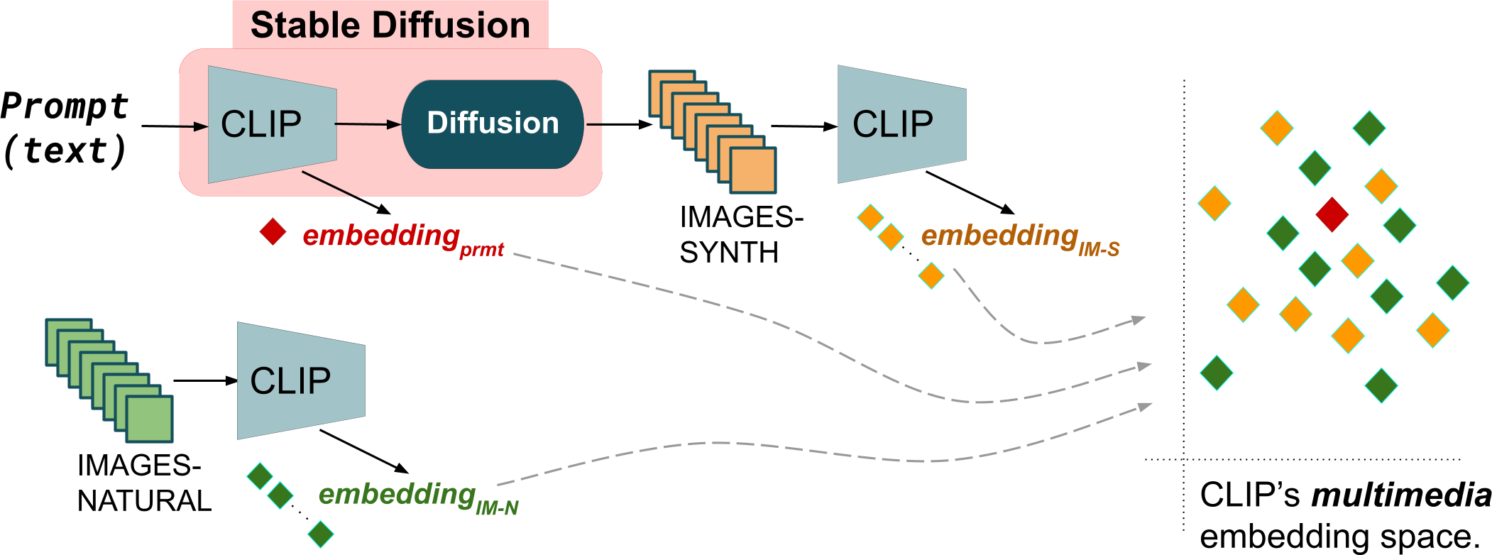
Figure 6: The prompt is passed to CLIP which yields an $embedding_{prmt}$ and guidance for SD. SD yields synthetic images (IM-S), which are passed back into CLIP to get $embeddings_{IM-S}$. Natural images (IM-N) are passed to CLIP which returns $embeddings_{IM-N}$. Right: All the embeddings (prompt, IM-N, IM-S) in the same, joint, embedding space.

The accuracy results are an effect of diversity; they are not, in themselves, a measure of diversity. Naive methods of directly measuring diversity of images by examining pixels intensities, or even summary stats such as eigenvectors (PCA, etc.) do not capture semantic content. Thankfully, modern language/image contrastive methods can provide a more meaningful measure. The CLIP model (Radford et al. 2021) is trained to create a joint high dimensional representation of both text and images; see Figure 6.

We utilize distances in the CLIP embeddings space to quantify diversity by computing centroids and summaries of image distances from them. For all of the images, we compute their CLIP embeddings, $E_{S,c}=ClipEmbedImage(I_{S,c})$ where $I_{S,c}$ are the images of set $S$ in class $c$. Because CLIP is trained using cosine similarity and relies on unit vectors, to calculate the centroid location of $E_{S,c}$, $M_{S,c}=uvec(\sum_{i}uvec(e_{S,c}^{i}\in E_{S,c}))$ where $uvec(\vec{v})=\frac{\vec{v}}{|\vec{v}|}$ is the unit vector function. Given the centroid, we then measure the Centroid Distance, the mean squared distance from that centroid to each image embedding, for each class $Distance_{S,c}=\sum_{i}\operatorname{codiff}(e_{S,c}^{i}\in E_{S,c},M_{S,c})^{2}/|E_{S,c}|$ where $\operatorname{codiff}$ is the complement of cosine similarity, $\operatorname{codiff}(x,y)=1-uvec(x)\cdot uvec(y)$, and for each set by averaging across classes.

The Centroid Distance for each set is shown in Figure 5. As expected, the Centroid Distance increases (gets more diverse), $Disamb$ $(1.23{\times}10^{-5})<$ $Disamb2.5$ $(2.05{\times}10^{-5})<$ $PromptAug$ $(2.49{\times}10^{-5})$. In comparison, ImageNet has greater diversity than all: $2.98{\times}10^{-5}$. This provides insight into the distribution of the samples and why some natural images are incorrectly classified when using the synthetic examples for training – the diversity of samples needed is simply not present in the synthetic sets.

We’ve seen that increasing diversity in synthetic training sets, either implicitly or explicitly, causes increased accuracy and that diversity can be measured using Centroid Distance. However, introducing too much diversity can lower accuracy. We will examine this in Reasons #3 & #4.

For comprehensiveness, we investigated two alternatives to Centroid Distance. First, to test if another embedding would work better, all of these results were recreated with Inception embeddings (Borji 2022); these are the embeddings derived from the penultimate layers of Inception networks trained to classify ImageNet. Inception embeddings did not provide any benefit to using CLIP embeddings and were not as applicable to non-ImageNet classes as the CLIP embeddings. Further, CLIP maps prompts to the same embedding space as images, a key feature that will be used in the next section.

Second, we applied the commonly used Frechet Distance (FD) $d^{2}=|\mu_{X}-\mu_{Y}|+tr(\sum_{X}+\sum_{Y}-2(\sum_{X}\sum_{Y})^{1/2})$. Instead of using FID Inception scores (Heusel et al. 2017), we substituted the CLIP embeddings. The first term of FD, subtracting centroids, strongly correlated with accuracy, but the second term, which compares across channels, did not. (Chong and Forsyth 2020) also found limitations in FID. As such, we use Centroid Distance going forward, which is also based on distances from centroids.

Reason #3: Diversity in Diffusion

In this section, we separate the effects of centroid-shift, measured as the difference in set centroids $\operatorname{codiff}(r_{1},r_{2})=1-uvec(r_{1})\cdot uvec(r_{2})$, and diversity on accuracy. We will also isolate the contribution of diffusion by expanding the use of Centroid Distance from the previous section. Recall that CLIP maps images and text prompts into the same space. Zero-shot classifiers using CLIP (Radford et al. 2021) find the nearest neighbor of an image embedding, the query, among the set of embeddings of the class prompts, the references (one for each of the 1000 classes).

Generalizing this, we allow both query and reference roles to be either prompts or images. Additionally, both prompts and images can have multiple instances per class. When the reference set has multiple instances ($N>1$) in a class, we replace those $N$ embeddings with their single centroid. The accuracy calculation is the same: a query is correct if its label matches the label of the nearest centroid’s class. Analagously to Centroid Distance, we’ll refer to this as Centroid Accuracy; see Figure 7. Formal notation is in Appendix A.

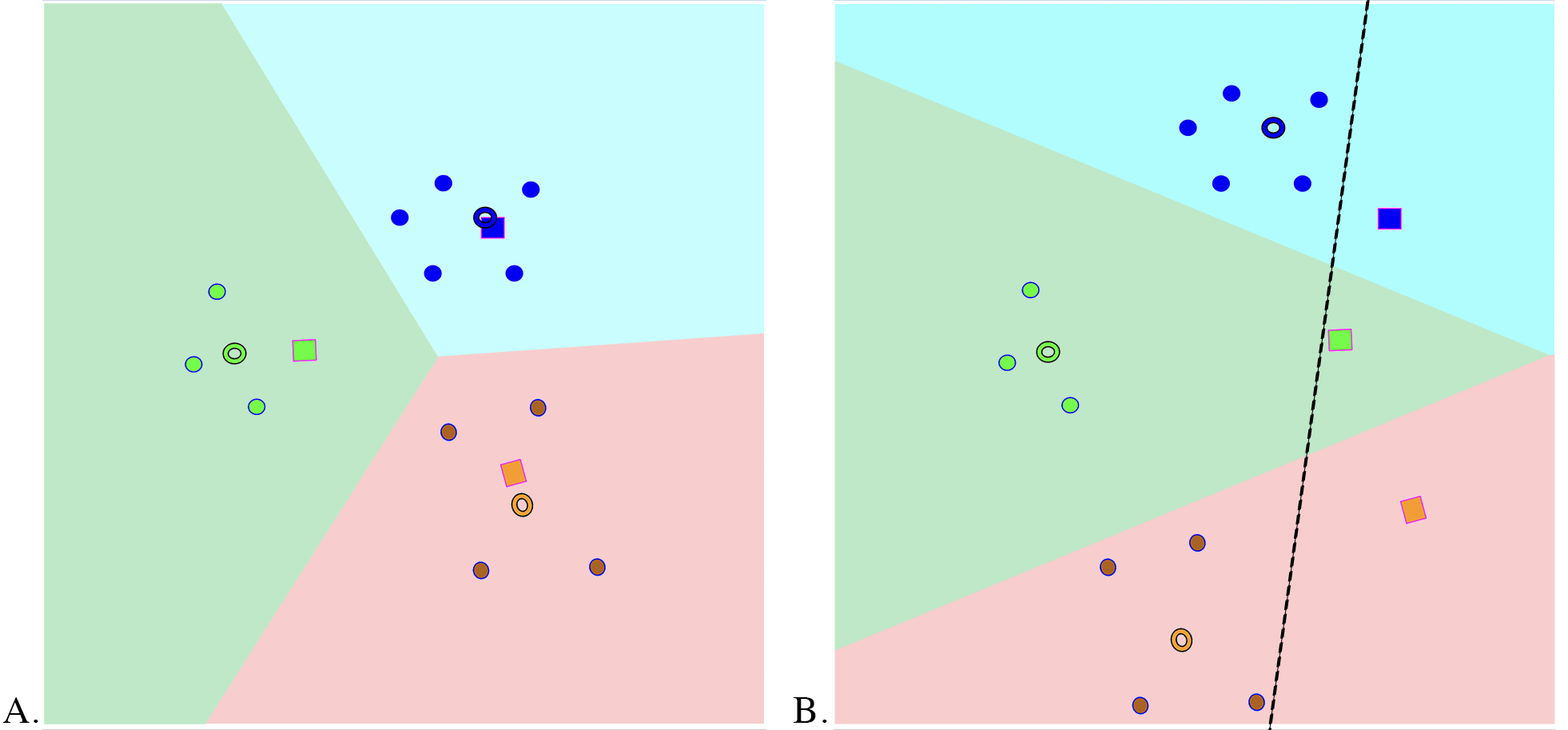
Figure 7: 3 clusters in the embedding space. Circles: images; donuts: centroid of the images; squares: text prompt. Left: Typical clustering. Red: images have higher diversity, but close centroid to the prompt. Blue: smaller distribution, and perfect centroid. Green: small diversity, but centroid is far from generating prompt (flawed, but similar images). Right: An alternate view, same matches, but all the prompts are linearly separated from all the images (discussed in Section 4).

We compute Centroid Accuracy on both images and prompts, distinguished with a -IM and -PRMT suffix respectively. Experiments include using the image-sets: ImageNet-IM, Disamb-IM, Disamb2.5-IM, PromptAug-IM, and the prompt-sets: Disamb2.5-PRMT, PromptAug-PRMT, as both query and reference. The full set of 36 classification trials is given in Appendix A; we will show the more informative ones as they are discussed. Whichever role is used (reference or query), references always use the set’s training split, and queries always uses an independent evaluation split.

In Table 3, Experiment 5 is the baseline, and is comparable to standard zero-shot learning where prompts are the reference set and the ImageNet-validation images are queries. The Centroid Accuracy for ImageNet (measured by the closest prompt to the image in the embedding space) is 70.1%.

Experiment 17 repeats the above experiment with Disamb2.5-IM as the queries to yield 74.9% accuracy. The 25.1% error can be decomposed into the portions caused by centroid-shift and by diversity. To ascertain the relative impact of each, another experiment is performed. Experiment 15 uses Disamb2.5-IM’s own centroid as the reference set rather than the prompts. By calculating the Centroid Accuracy using the same distributions of reference and query, only errors due to diversity remain. If diffusion created images with little/no diversity, then every image would map back to the centroid and Centroid Accuracy would be 100%. However, accuracy is 82.0% (18.0% error), indicating diffusion’s diversity is large enough that some images are closer to the centroids of other classes. Comparing this to the 25.1% error when using prompts as references, because only the centroid has changed between experiments, the difference in the errors is attributable to a centroid-shift. A centroid-shift within the CLIP embedding space is a shift in the concept that is represented – a meaning-shift.

Reference	Query	Centroid	Avg Cos.	Exp
Set	Set	Accuracy	Similarity	#
Disamb2.5-PRMT	ImageNet-IM	70.1%	0.2425	5
Disamb2.5-PRMT	Disamb2.5-IM	74.9%	0.2421	17
Disamb2.5-IM	Disamb2.5-IM	82.0%	0.8709	15

Table 3: Centroid Accuracies. Experiment #’s index to the full set of 36 {reference$\times$query} tests. Full list in Appendix A.

Returning to Experiment 15, a second interesting aspect is that we can attribute the 18.0% misclassification to diversity introduced by diffusion rather than CLIP. We know this because the images are all created from the same prompt; therefore, diffusion is the only source of variation in the generative process. This is an accuracy-based measure of the $Distance_{Disamb2.5}=2.05{\times}10^{-5}$ from Figure 5.

So far, in this section, to quantify the effects of centroid-shift vs. diversity, we modified the role of the synthetic images to use them as the query set. We determined that both a shift between the centroids of the synthetic images and diversity of the synthetic images reduces Centroid Accuracy with the latter contributing more to the overall error.

This puts Reason #2 in context. In Reason #2, we needed to add diversity to improve the ResNet accuracies (Tables 1&2). Here, we showed that just adding diversity is not a panacea; the images generated must still accurately represent the underlying prompt — which the diffusion process does not guarantee. This is why augmentations, such as in PromptAug, are used; they explicitly guide diversity by providing hints to diffusion about how to create unique, but meaningful, images. The augmentations did, on average, improve accuracy; useful diversity was added. In a few classes, however, the errors from centroid-shift dominated the performance and the prompt embedding from CLIP did not represent the class. This failure mode is described in the next section.

On a pragmatic note, we observe that the diffusion process has varying levels of success in paying attention to all portions of specific prompts. Because of the popularity of TTI systems, the practice of prompt tuning (Hao et al. 2022; Zhou et al. 2022; Andruszków 2023) has become widespread; this is the colloquial name given to the explicit control of mean and diversity. In Appendix B, we provide illustrative examples of prompts that do exactly as intended; they control diversity by narrowing the subject/background (the “school bus” class). To contrast this, we also present a class for which diffusion has difficulty; it only creates a canonical version of the subject (“quail”).

Reason #4: Delving Deeper into Centroid-Shifts

To begin this section, recall that Experiment 5 in Table 3 achieved a Centroid Accuracy of 70.1%. This performance indicates a reasonable match between the concept (text/class prompt) as encoded by CLIP and the ImageNet images (when also encoded by CLIP). Diversity, as shown in the previous section, has a larger contribution to error than centroid-shift.

Nonetheless, centroid-shifts can be largely detrimental to some individual classes. To see this effect, we examine classes that SD is unable to generate. Two such classes are “hammer” and “nail”; see Figure 8. The synthetic images for “hammer” are largely nonsensical – not resembling any coherent object. In contrast, the synthetic images for “nail” represent real objects (screws, nuts and bolts), but not the desired class, “nail.” How do these two different failure modes manifest themselves in our analysis? Table 4 shows the accuracy for these two classes.

hammer
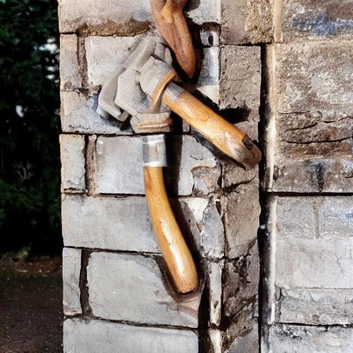
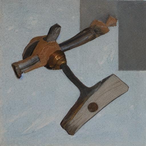
nail

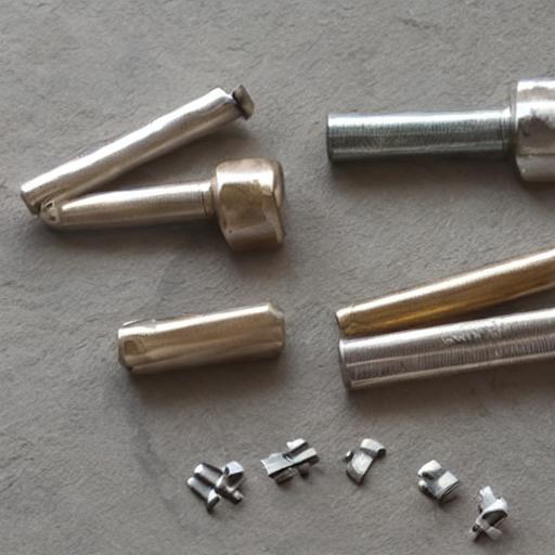
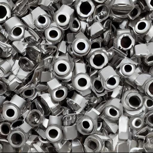
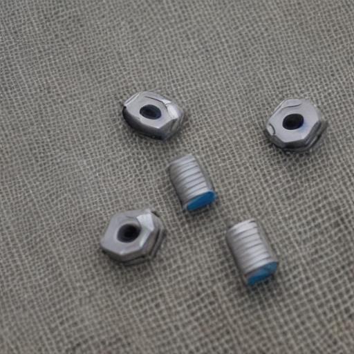
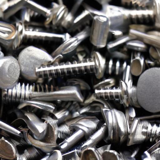
Figure 8: Two example classes where the generated images are poor: "hammer" (top) and "nail" (bottom).

Looking at the poor results for hammer, we can ask whether diffusion’s generation is to blame, or is the concept “hammer” incorrectly represented in CLIP? To determine this, we set the reference set to Disamb2.5-PRMT (which includes “hammer”) and first lookup the natural ImageNet-IM images. The accuracy is only 14% (Table 4, line 1) for this class, significantly lower than the average across all classes of 70.1%. Simply put, CLIP does not represent the prompt well. The embedding CLIP produced, which should represent the concept “hammer”, erroneously represents a different concept. Additionally, we can ask whether diffusion is able to accurately recreate the concept that is represented. Changing the query set to the synthesized images (line 2) does not improve performance; the diversity from diffusion places images so far from their centroid that they are in a different class.

Next, we repeat the same test for “nail.” As before, first we set the reference set to the Disamb2.5-PRMT and lookup the natural ImageNet “nail” images. As with hammers, the accuracy is lower than the average (58%). Next, we ask whether diffusion is able to accurately recreate whatever concept CLIP produced for “nail.” Interestingly, the accuracy jumps to 84%. Contrast this with the 16% for “hammer” in the same test. This indicates that, although the concept of “nail” may not be represented as accurately as other classes, the synthetic images generated by diffusion are consistent with CLIP’s flawed prompt embedding — even though they are not close to the ImageNet “nail” images. This error is largely attributable to a centroid-shift between the synthesized and ImageNet images.

In summary,“nail” and “hammer” are failure examples where the system would benefit from an improved CLIP model. In fact, recently, (Wortsman 2023) employed an improved CLIP model that improves the zero-shot to 80.1% (competitive with our ResNet-RS-152 at 80.8%; Table 1).

Reference	Query	Avg.	Hammer	Nail
Set	Set	CA	CA	CA
Disamb2.5-PRMT	ImageNet-IM	70.1	14.0	58.0
Disamb2.5-PRMT	Disamb2.5-IM	74.9	16.0	84.0

Table 4: Centroid Accuracy (CA) results for “nail” and “hammer” indicate different failure modes. The Avg. CA column give the average accuracy across all 1000 classes.

4 Geometry of Embeddings

In the previous section, we concentrated on Centroid Accuracy for classification. In this section, we take a closer look at the cosine similarity scores it is based on. We reveal some surprising findings in the underlying geometry of CLIP’s shared embeddings space for prompts and images.

When we examine the magnitudes of the similarities between prompts and other prompts (Table 5, Experiments 30,36,29) the similarity is high (0.70-0.90). The same is true with the similarity of images (Experiments 22,15). Now, let us examine the similarity across modalities: between prompts and images. There is a dramatic drop in similarity without a correspondingly large drop in accuracy.

There seems to be a set of clusters that are prompts and another that are images. Within the clusters, however, the individual classes are oriented such that the classification across modalities is still possible. We attempted to visualize this. To do so, we first wanted to examine if there was a clean separation between the set of prompt embeddings and the set of image embeddings. To our surprise, there was not only a separation, but the two types of embeddings were linearly separable. A potential way to have them linearly separable, while still useful for classification, is shown in Figure 7B.

		Centroid	Avg Cos.	Exp
Reference Set	Query Set	Accu-	Simi-	#
		racy	larity
PromptAug-PRMT	PromptAug-PRMT	100%	0.878	30
PromptAug-PRMT	Disamb2.5-PRMT	99.6%	0.796	36
Disamb2.5-PRMT	PromptAug-PRMT	98.8%	0.699	29
PromptAug-IM	PromptAug-IM	70.5%	0.852	22
Disamb2.5-IM	Disamb2.5-IM	82.0%	0.871	15
Disamb2.5-PRMT	Disamb2.5-IM	74.9%	0.242	17
Disamb2.5-PRMT	PromptAug-IM	62.4%	0.231	23
PromptAug-PRMT	Disamb2.5-IM	76.2%	0.258	18
PromptAug-PRMT	PromptAug-IM	69.2%	0.261	24

Table 5: Measures within and across text & image modalities.

Examining CLIP’s loss function provides insight into how this occurs. The loss function rewards correct pairings of prompt and image, but does not attempt to create the same representation for the pair. This explains how this result is possible, though it remains quite unexpected. Recently, (Huang and Alon 2023) have also discovered this.

5 k-nn vs Centroid Accuracy

Zero-shot classification typically employs a single point, the prompt embedding of each class label, as references vectors. This effectively creates a k-nn classifier with $k=1$. Directly relating to our discussions of class diversity, the collapsing of the reference set to a single point may mask the shape and extent of the full reference set. If we expand to the general k-nn approach, this potential loss of information is no longer necessary. This is especially relevant to the scenarios where the reference set is comprised of labeled images or where unique prompts (PromptAug) are used. We repeat the entire set of experiments without collapsing the reference set to centroids, and instead find the nearest (highest cosine similarity) $k$ reference set embeddings. The most frequent class of the found $k$ is returned as the label. We test $k=1,5$.

Though we do not have the space to delve into the details of the 60 k-nn experiments, the full results are in Table 6 (Appendix A). Across the numerous combinations of reference and query sets, Centroid Accuracy averages to 77.1% while k-nn $k=1$ accuracy is 74.6% and $k=5$ is 77.3%. $k=5$ was better than Centroid Accuracy in 40% of the experiments.

This is consistent with the findings presented so far. Without averaging, when using the single nearest neighbor, if the reference set produces imperfect examples, performance can degrade. However, when the labels of a few samples are considered, the effect is mitigated. The results indicate that here, reference centroids sufficiently summarized the statistic required for classification. Additionally, on a pragmatic note, Centroid Accuracy performs similarly to $k=5$ and it is computationally far less expensive (needing to consider 1000 centroids vs. 1.2M neighboring images). In the future, it remains an open question of whether more sophisticated methods beyond k-nn can be used to better exploit the distributions of the individual examples.

6 Discussion

The last few years have seen an explosion in both the number of TTI systems and their improvement in quality. Rapid innovation has taken place in all aspects of the systems: the underlying large language model, the generation process, the memory requirements and the computational speed. Despite, or perhaps because of, the rate of innovation coupled with the already well-understood mathematical underpinning of the diffusion process, comparatively little work has been devoted to developing an understanding about what can be generated. Though the synthetic images already often appear indistinguishable from natural ones, they are not suitable for training classifiers. This indicates that the set of generated images does not yet represent the set of natural images. We examined the roles of diversity and centroid-shifts in both the CLIP and diffusion processes. Our findings include:

1. Ambiguity in prompt interpretation hinders training with synthetic images. It can be mitigated by revising prompts to better reflect the class semantics. This is not merely a matter of synonyms and homonyms – the target class may itself have a bias that is not represented in the prompt.

2. The influence of the prompt must be carefully controlled. Allowing a high influence does not allow for sufficient diversity when creating new datasets (Table 1). Reducing the influence increases diversity (Figure 5), which can improve their utility in training (Table 2). However, increasing diversity has limits. Coherence and accuracy of the images can drop as diversity increases. As demonstrated, a few classes increased diversity too much – e.g. to the point where they are no longer accurate (Table 4) and are, therefore, no longer useful in training.

3. Accuracy is affected by both centroid-shift and diversity. Our Centroid Accuracy and Centroid Distance techniques in combination isolate the effects of diversity and show that diversity has a larger impact on accuracy than centroid-shift. In addition, the effects of the CLIP and diffusion processes can be measured separately. Diffusion is a larger contributor to error than CLIP.

4. For most classes, CLIP faithfully reproduces the concepts; it largely represents ImageNet’s interpretation. Nonetheless, a potential failure case for any TTI system is its inability to recreate images for some prompts/concepts. We presented examples where CLIP represented nonsensical concepts as well as incorrect concepts.

5. In terms of CLIP’s representation of text and images, we have found that the embeddings are linearly separable — an intuitively surprising finding as successful zero-shot classifiers and most clustering is rarely visualized as such. This explains why prompts that are internally consistent when embedded do not always translate to internally consistent images when used by diffusion.

Our study has used Stable Diffusion, the most commonly used TTI system; however, any generation system can be easily substituted. We hope that this work provides insights into image generation systems and also provides guidelines for the understanding, analysis, and evaluation of new systems as they are rapidly deployed.

Appendix A Appendix: Centroid Accuracies and k-nn 

Experiment	Reference	Query	Centroid	k-nn k=1	k-nn k=5	Avg Cos.
#	Set	Set	Accuracy	Accuracy	Accuracy	Similarity
1	ImageNet-IM	ImageNet-IM	75.1%	76.3%	79.2%	0.8353
2	Disamb-IM	ImageNet-IM	60.8%	60.9%	63.1%	0.7748
3	Disamb2.5-IM	ImageNet-IM	61.2%	59.4%	62.5%	0.7779
4	PromptAug-IM	ImageNet-IM	61.4%	58.3%	62.0%	0.7762
5	Disamb2.5-PRMT	ImageNet-IM	70.1%	70.1%	70.1%	0.2425
6	PromptAug-PRMT	ImageNet-IM	73.9%	72.4%	72.8%	0.2600
7	ImageNet-IM	Disamb-IM	76.6%	71.2%	75.3%	0.8388
8	Disamb-IM	Disamb-IM	82.0%	95.5%	96.3%	0.9685
9	Disamb2.5-IM	Disamb-IM	89.8%	89.5%	91.3%	0.8869
10	PromptAug-IM	Disamb-IM	82.5%	82.1%	84.9%	0.8658
11	Disamb2.5-PRMT	Disamb-IM	86.3%	86.3%	86.3%	0.2560
12	PromptAug-PRMT	Disamb-IM	86.2%	85.3%	85.4%	0.2675
13	ImageNet-IM	Disamb2.5-IM	66.0%	58.8%	63.5%	0.8072
14	Disamb-IM	Disamb2.5-IM	78.1%	81.1%	82.8%	0.8518
15	Disamb2.5-IM	Disamb2.5-IM	82.0%	80.8%	83.9%	0.8709
16	PromptAug-IM	Disamb2.5-IM	76.7%	72.7%	76.9%	0.8564
17	Disamb2.5-PRMT	Disamb2.5-IM	74.9%	74.9%	74.9%	0.2421
18	PromptAug-PRMT	Disamb2.5-IM	76.2%	74.2%	74.5%	0.2580
19	ImageNet-IM	PromptAug-IM	55.8%	49.3%	53.7%	0.7874
20	Disamb-IM	PromptAug-IM	59.2%	60.5%	62.6%	0.8136
21	Disamb2.5-IM	PromptAug-IM	61.7%	61.2%	64.3%	0.8375
22	PromptAug-IM	PromptAug-IM	70.5%	65.6%	70.3%	0.8518
23	Disamb2.5-PRMT	PromptAug-IM	62.4%	62.4%	62.4%	0.2314
24	PromptAug-PRMT	PromptAug-IM	69.2%	67.5%	67.9%	0.2605
25	ImageNet-IM	PromptAug-PRMT	93.1%	80.1%	88.0%	0.2742
26	Disamb-IM	PromptAug-PRMT	92.9%	83.1%	88.0%	0.2596
27	Disamb2.5-IM	PromptAug-PRMT	93.0%	80.4%	87.1%	0.2596
28	PromptAug-IM	PromptAug-PRMT	96.3%	80.5%	89.4%	0.2684
29	Disamb2.5-PRMT	PromptAug-PRMT	98.8%	98.8%	98.8%	0.6991
30	PromptAug-PRMT	PromptAug-PRMT	100%	100%	100%	0.8776
31	ImageNet-IM	Disamb2.5-PRMT	95.4%	n/a	n/a	0.2919
32	Disamb-IM	Disamb2.5-PRMT	98.0%	n/a	n/a	0.2824
33	Disamb2.5-IM	Disamb2.5-PRMT	98.5%	n/a	n/a	0.2770
34	PromptAug-IM	Disamb2.5-PRMT	96.6%	n/a	n/a	0.2720
35	Disamb2.5-PRMT	Disamb2.5-PRMT	100%	n/a	n/a	1.0000
36	PromptAug-PRMT	Disamb2.5-PRMT	99.6%	n/a	n/a	0.7960
Averages (only rows with k-nn )			77.1%	74.6%	77.3%

Table 6: For all pairs of reference and query sets, we give the Centroid Accuracy, k-nn Accuracy using $\emph{k-}nn~{}=\{1,5\}$ and Average Cosine Similarity. For k-nn , Disamb2.5-PRMT queries are not calculated because of small sample sizes.

For this study, we experimented with a large set of reference and query sets; many more than could be presented in the main text. Results are presented here. We compute Centroid Accuracy on both images and prompts, distinguished with a -IM and -PRMT suffix respectively. Experiments include the image-sets: ImageNet-IM, Disamb-IM, Disamb2.5-IM, PromptAug-IM, and the prompt-sets: Disamb2.5-PRMT, PromptAug-PRMT, for a total of 36 experiments.

The calculation of Centroid Accuracy proceeds from Section 3. For all of the images, we compute their CLIP embeddings, $E_{S,c}=ClipEmbedImage(I_{S,c})$ where $I_{S,c}$ are the images of set $S$ in class $c$. Because CLIP is trained using cosine similarity and relies on unit vectors, to calculate the centroid location of $E_{S,c}$, $M_{S,c}=uvec(\sum_{i}uvec(e_{S,c}^{i}\in E_{S,c}))$ where $uvec(\vec{v})=\frac{\vec{v}}{|\vec{v}|}$ is the unit vector function. The set of class centroids for the reference set, one per class, is $R^{c}$.

The nearest reference embedding in the set $R^{c}$ to a query embedding $q$ is $Near(q,R^{c})=n\text{~{}where~{}}n\in R^{c}$; randomly selected in case of ties.

The classification correctness of an individual query, $q$, is $Z(q,R)$. $Z(q,R)=1.0$ when $Near(q,R^{c})$ is labeled with the same class as $q$, otherwise $Z(q,R)=0.0$.

The Centroid Accuracy, $\mathop{\textnormal{CA}}\nolimits$, for a query set $Q$ and reference set $R$ is then $\mathop{\textnormal{CA}}\nolimits(Q,R)=\frac{\sum_{q\in Q}Z(q,R)}{|Q|}$.

In Section 5, we discussed using a more general k-nn approach to the zero-shot centroid based versions described earlier. Results with $k=1,5$ are also presented in the table. As with Centroid Accuracy, references always use the set’s training split, and queries always uses an independent evaluation split. k-nn specifics are described in Section 5.

Finally, in the last column, we show the average Cosine Similarity; this is the average of the cosine similarities of the query-reference embedding pairs. These are discussed in detail in the main text, Section 4.

Appendix B Appendix: Explicit Control of Diversity and Mean-Shift through Prompt-Tuning

We briefly examine the common practice (from both academia and end-users of Stable Diffusion) of fine-tuning prompts to produce broader or narrower sets of images. We examine the effects that common prompt tuning has on variance and centroid-shift using the prompt “school bus” and three modified school bus queries. For each of the four prompts (shown in Figure 9), we synthesize 1200 new images; these will be used as the query images. The reference set, which we hold constant, is Disamb2.5-IM; this makes the experiments comparable to Experiment 15 (shown in Appendix A. As a reminder, recall that “school bus” is a class in ImageNet (and therefore in Disamb2.5).

Query	Sample Images	Accuracy
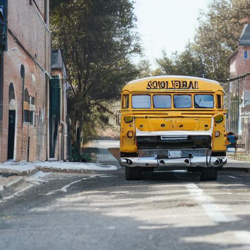
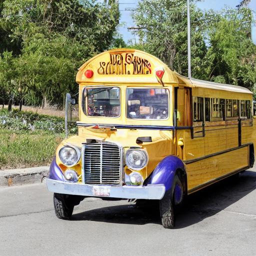
school bus		92.5%
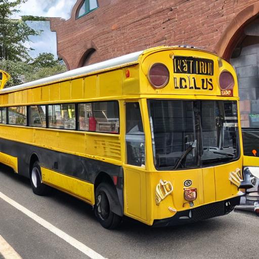
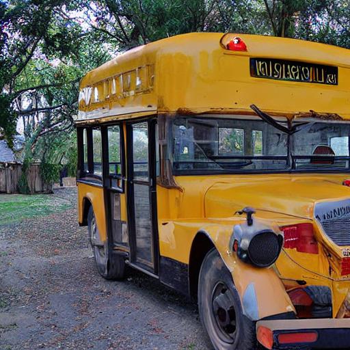
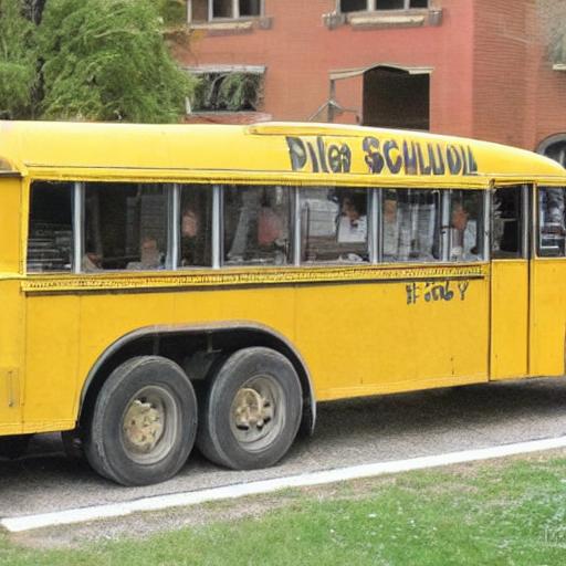
yellow school bus		96.2%
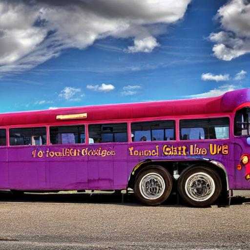
purple school bus		90.7%
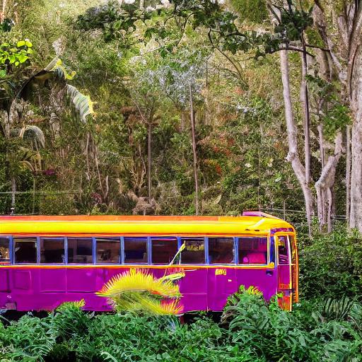
purple school bus in a jungle		88.2%

Figure 9: Centroid Accuracy for the query using “school bus” as the reference.

The new set of images created with the base prompt “school bus” is first tested. Like Experiment 15, this measures only the diversity, entirely due to diffusion since the query text has not changed, and results in Centroid Accuracy of 92.5%.

Next, we attempt to explicitly reduce diversity by constraining the color. The query “yellow school bus” reduces the diversity of school buses generated. Since yellow is the color most often associated with school buses, this will likely have minimal impact on the centroid of the synthetic images, but rather serve primarily to reduce diversity. The increased accuracy of 96.2% corroborates this. Measuring the Centroid Distance produces $10.96{\times}10^{-4}$ for “school bus” and $5.33{\times}10^{-4}$ for “yellow school bus”, verifying the reduced diversity of the latter.

Next, we shift the mean of the synthetic images by generating uncommon school buses, e.g. “purple school buses.” Earlier, we suggested the diffusion process is heavily influenced by the underlying image distributions of the training data; the more common the object, the more likely it is to be produced. Since purple school buses are less likely to be encountered than yellow, they appear less frequently in the reference set, and therefore may be less accurately classified when used as queries. With respect to the reference school bus images, we expect a shift in the centroid of the synthetic images (centroid-shift). Correspondingly, we see reduced classification accuracy (90.7%). Finally, we can further increase centroid-shift by additionally constraining the background to an unlikely scenario: “purple school bus in a jungle,” this further reduces accuracy (88.2%). Additionally, this prompt changes the diversity by limiting the backgrounds generated.

We would be remiss in presenting these results without discussing pragmatic limitations of prompt tuning. Recall that in our set with augmented prompts, PromptAug, we generated a unique prompt for each image generated. The modified prompts used a variety of prefix and postfix modifiers to the class label. In general, these did improve the diversity of the images generated. However, for some classes, not all of the modifiers in the prompts were present. Instead, only similar images were created, despite the modifiers that were used. See Figure 10. This is commonly witnessed by end-users who carefully tune prompts to find the words and phrases that “make it to” the image.

Set	Sample Images
Disamb2.5
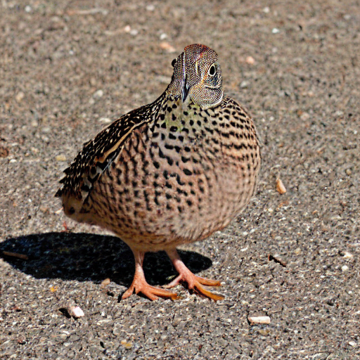
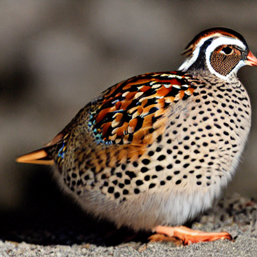
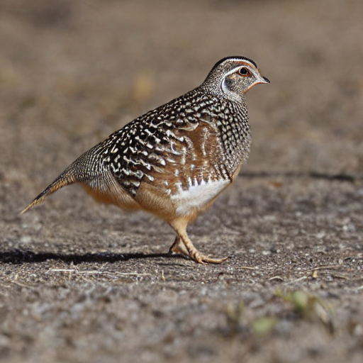
PromptAug

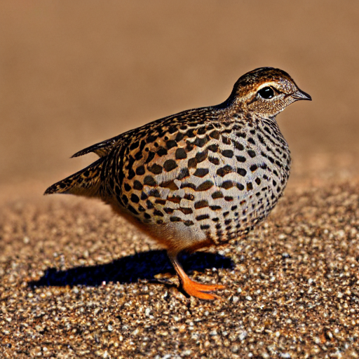
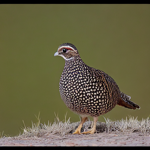
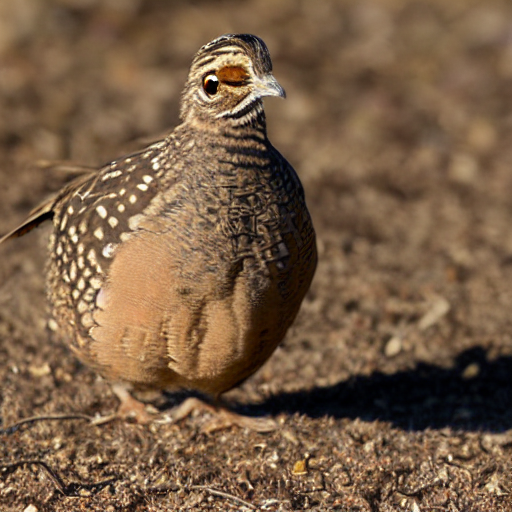
1. beautiful, common, extremely small quail, with many other other objects visible. Hyper-sharp.

2. old, common, extremely large size quail, centered in the image. Typical snapshot.

3. ugly, extremely uncommon, slightly small size quail, centered in the image. Hyper-sharp.

Figure 10: Top row all generated with prompt "quail". Bottom row, generated with the prompts shown. There is some added diversity compared to the top row, but parts of the prompts are not captured in the image generation.

References

- Andruszków (2023) Andruszków, K. 2023. All-In-One Guide For Midjourney: The Art Of Prompts. https://bowwe.com/en/blog/guide-to-midjourney-prompts. Accessed: 2023-08-119.
- Athalye (2020) Athalye, A. 2020. https://github.com/anishathalye/imagenet-simple-labels. Accessed: 2023-07-26.
- Azizi et al. (2023) Azizi, S.; Kornblith, S.; Saharia, C.; Norouzi, M.; and Fleet, D. J. 2023. Synthetic Data from Diffusion Models Improves ImageNet Classification. arXiv:2304.08466.
- Bansal and Grover (2023) Bansal, H.; and Grover, A. 2023. Leaving Reality to Imagination: Robust Classification via Generated Datasets. arXiv:2302.02503.
- Beyer et al. (2020) Beyer, L.; Hénaff, O. J.; Kolesnikov, A.; Zhai, X.; and van den Oord, A. 2020. Are we done with ImageNet? arXiv:2006.07159.
- Bhattarai et al. (2020) Bhattarai, B.; Baek, S.; Bodur, R.; and Kim, T. 2020. Sampling Strategies for GAN Synthetic Data. In 2020 IEEE International Conference on Acoustics, Speech and Signal Processing, ICASSP 2020, Barcelona, Spain, May 4-8, 2020, 2303–2307. IEEE.
- Borji (2022) Borji, A. 2022. Pros and cons of GAN evaluation measures: New developments. Computer Vision and Image Understanding, 215: 103329.
- Chang et al. (2023) Chang, H.; Zhang, H.; Barber, J.; Maschinot, A.; Lezama, J.; Jiang, L.; Yang, M.-H.; Murphy, K.; Freeman, W. T.; Rubinstein, M.; Li, Y.; and Krishnan, D. 2023. Muse: Text-To-Image Generation via Masked Generative Transformers. arXiv:2301.00704.
- Chen et al. (2023) Chen, W.; Wu, J.; Xie, P.; Wu, H.; Li, J.; Xia, X.; Xiao, X.; and Lin, L. 2023. Control-A-Video: Controllable Text-to-Video Generation with Diffusion Models. arXiv:2305.13840.
- Chong and Forsyth (2020) Chong, M. J.; and Forsyth, D. 2020. Effectively unbiased fid and inception score and where to find them. In Proceedings of the IEEE/CVF conference on computer vision and pattern recognition, 6070–6079.
- Deng et al. (2009) Deng, J.; Dong, W.; Socher, R.; Li, L.; Li, K.; and Fei-Fei, L. 2009. ImageNet: A large-scale hierarchical image database. In 2009 IEEE Computer Society Conference on Computer Vision and Pattern Recognition (CVPR 2009), 20-25 June 2009, Miami, Florida, USA, 248–255. IEEE Computer Society.
- Dewi et al. (2021) Dewi, C.; Chen, R.; Liu, Y.; Jiang, X.; and Hartomo, K. D. 2021. Yolo V4 for Advanced Traffic Sign Recognition With Synthetic Training Data Generated by Various GAN. IEEE Access, 9: 97228–97242.
- Dhariwal and Nichol (2021) Dhariwal, P.; and Nichol, A. Q. 2021. Diffusion Models Beat GANs on Image Synthesis. In Ranzato, M.; Beygelzimer, A.; Dauphin, Y. N.; Liang, P.; and Vaughan, J. W., eds., Advances in Neural Information Processing Systems 34: Annual Conference on Neural Information Processing Systems 2021, NeurIPS 2021, December 6-14, 2021, virtual, 8780–8794.
- Ding et al. (2021) Ding, M.; Yang, Z.; Hong, W.; Zheng, W.; Zhou, C.; Yin, D.; Lin, J.; Zou, X.; Shao, Z.; Yang, H.; et al. 2021. Cogview: Mastering text-to-image generation via transformers. Advances in Neural Information Processing Systems, 34: 19822–19835.
- Gal et al. (2022) Gal, R.; Alaluf, Y.; Atzmon, Y.; Patashnik, O.; Bermano, A. H.; Chechik, G.; and Cohen-Or, D. 2022. An image is worth one word: Personalizing text-to-image generation using textual inversion. arXiv preprint arXiv:2208.01618.
- Garden (2023) Garden, M. 2023. TF-Vision Model Garden. https://github.com/tensorflow/models/blob/master/official/vision/MODEL_GARDEN.md. Accessed: 2023-08-04.
- Goodfellow et al. (2020) Goodfellow, I.; Pouget-Abadie, J.; Mirza, M.; Xu, B.; Warde-Farley, D.; Ozair, S.; Courville, A.; and Bengio, Y. 2020. Generative adverserial networks. Communications of the ACM, 63(11): 139–144.
- Hao et al. (2022) Hao, Y.; Chi, Z.; Dong, L.; and Wei, F. 2022. Optimizing prompts for text-to-image generation. arXiv preprint arXiv:2212.09611.
- Heusel et al. (2017) Heusel, M.; Ramsauer, H.; Unterthiner, T.; Nessler, B.; and Hochreiter, S. 2017. GANs Trained by a Two Time-Scale Update Rule Converge to a Local Nash Equilibrium. In Guyon, I.; Luxburg, U. V.; Bengio, S.; Wallach, H.; Fergus, R.; Vishwanathan, S.; and Garnett, R., eds., Advances in Neural Information Processing Systems, volume 30. Curran Associates, Inc.
- Ho, Jain, and Abbeel (2020) Ho, J.; Jain, A.; and Abbeel, P. 2020. Denoising Diffusion Probabilistic Models. In Larochelle, H.; Ranzato, M.; Hadsell, R.; Balcan, M.; and Lin, H., eds., Advances in Neural Information Processing Systems 33: Annual Conference on Neural Information Processing Systems 2020, NeurIPS 2020, December 6-12, 2020, virtual.
- Huang and Alon (2023) Huang, J.; and Alon, Y. 2023. Embeddings in CLIP (working title). In Forthcoming.
- iNaturalist (2023) iNaturalist. 2023. A Community for Naturalists. http://iNaturalist.org. Accessed: 2023-08-04.
- Kang et al. (2023) Kang, M.; Zhu, J.-Y.; Zhang, R.; Park, J.; Shechtman, E.; Paris, S.; and Park, T. 2023. Scaling up GANs for Text-to-Image Synthesis. In Proceedings of the IEEE Conference on Computer Vision and Pattern Recognition (CVPR).
- Kong et al. (2021) Kong, Z.; Ping, W.; Huang, J.; Zhao, K.; and Catanzaro, B. 2021. DiffWave: A Versatile Diffusion Model for Audio Synthesis. In 9th International Conference on Learning Representations, ICLR 2021, Virtual Event, Austria, May 3-7, 2021. OpenReview.net.
- Miller (1995) Miller, G. A. 1995. WordNet: a lexical database for English. Communications of the ACM, 38: 39–41.
- Nichol et al. (2022) Nichol, A.; Dhariwal, P.; Ramesh, A.; Shyam, P.; Mishkin, P.; McGrew, B.; Sutskever, I.; and Chen, M. 2022. GLIDE: Towards Photorealistic Image Generation and Editing with Text-Guided Diffusion Models. arXiv:2112.10741.
- Pratt, Liu, and Farhadi (2022) Pratt, S.; Liu, R.; and Farhadi, A. 2022. What does a platypus look like? Generating customized prompts for zero-shot image classification. arXiv:2209.03320.
- PromptHero (2023) PromptHero. 2023. Openjourney. https://openjourney.art/. Accessed: 2023-08-05.
- Radford et al. (2021) Radford, A.; Kim, J. W.; Hallacy, C.; Ramesh, A.; Goh, G.; Agarwal, S.; Sastry, G.; Askell, A.; Mishkin, P.; Clark, J.; et al. 2021. Learning transferable visual models from natural language supervision. In International Conference on Machine Learning, 8748–8763. PMLR.
- Ramesh et al. (2022) Ramesh, A.; Dhariwal, P.; Nichol, A.; Chu, C.; and Chen, M. 2022. Hierarchical text-conditional image generation with clip latents. arXiv preprint arXiv:2204.06125.
- Rombach et al. (2021) Rombach, R.; Blattmann, A.; Lorenz, D.; Esser, P.; and Ommer, B. 2021. High-Resolution Image Synthesis with Latent Diffusion Models. arXiv:2112.10752.
- Ruiz et al. (2023) Ruiz, N.; Li, Y.; Jampani, V.; Pritch, Y.; Rubinstein, M.; and Aberman, K. 2023. Dreambooth: Fine tuning text-to-image diffusion models for subject-driven generation. In Proceedings of the IEEE/CVF Conference on Computer Vision and Pattern Recognition, 22500–22510.
- Saharia et al. (2022) Saharia, C.; Chan, W.; Saxena, S.; Li, L.; Whang, J.; Denton, E.; Ghasemipour, S. K. S.; Ayan, B. K.; Mahdavi, S. S.; Lopes, R. G.; Salimans, T.; Ho, J.; Fleet, D. J.; and Norouzi, M. 2022. Photorealistic Text-to-Image Diffusion Models with Deep Language Understanding.
- Sankaranarayanan et al. (2018) Sankaranarayanan, S.; Balaji, Y.; Jain, A.; Lim, S. N.; and Chellappa, R. 2018. Learning From Synthetic Data: Addressing Domain Shift for Semantic Segmentation. In 2018 IEEE Conference on Computer Vision and Pattern Recognition, CVPR 2018, Salt Lake City, UT, USA, June 18-22, 2018, 3752–3761. Computer Vision Foundation / IEEE Computer Society.
- Sariyildiz et al. (2023) Sariyildiz, M. B.; Alahari, K.; Larlus, D.; and Kalantidis, Y. 2023. Fake it till you make it: Learning transferable representations from synthetic ImageNet clones. arXiv:2212.08420.
- Song, Meng, and Ermon (2021) Song, J.; Meng, C.; and Ermon, S. 2021. Denoising Diffusion Implicit Models. In 9th International Conference on Learning Representations, ICLR 2021, Virtual Event, Austria, May 3-7, 2021. OpenReview.net.
- Stock and Cisse (2018) Stock, P.; and Cisse, M. 2018. ConvNets and ImageNet Beyond Accuracy: Understanding Mistakes and Uncovering Biases. In Proceedings of the European Conference on Computer Vision (ECCV).
- Tewel et al. (2023) Tewel, Y.; Gal, R.; Chechik, G.; and Atzmon, Y. 2023. Key-Locked Rank One Editing for Text-to-Image Personalization. arXiv:2305.01644.
- Tsipras et al. (2020) Tsipras, D.; Santurkar, S.; Engstrom, L.; Ilyas, A.; and Madry, A. 2020. From ImageNet to Image Classification: Contextualizing Progress on Benchmarks. In III, H. D.; and Singh, A., eds., Proceedings of the 37th International Conference on Machine Learning, volume 119 of Proceedings of Machine Learning Research, 9625–9635. PMLR.
- Wortsman (2023) Wortsman, M. 2023. Reaching 80% Zero-Shot Accuracy with OpenClip: VIT-G/14 Trained on LAION-2B. https://laion.ai/blog/giant-openclip/. Accessed: 2023-08-09.
- Xie et al. (2016) Xie, S.; Girshick, R. B.; Dollár, P.; Tu, Z.; and He, K. 2016. Aggregated Residual Transformations for Deep Neural Networks. 2017 IEEE Conference on Computer Vision and Pattern Recognition (CVPR), 5987–5995.
- Xu et al. (2023) Xu, X.; Wang, Z.; Zhang, E.; Wang, K.; and Shi, H. 2023. Versatile Diffusion: Text, Images and Variations All in One Diffusion Model. arXiv:2211.08332.
- Yu et al. (2022) Yu, J.; Xu, Y.; Koh, J. Y.; Luong, T.; Baid, G.; Wang, Z.; Vasudevan, V.; Ku, A.; Yang, Y.; Ayan, B. K.; et al. 2022. Scaling autoregressive models for content-rich text-to-image generation. arXiv preprint arXiv:2206.10789.
- Zhou et al. (2022) Zhou, K.; Yang, J.; Loy, C. C.; and Liu, Z. 2022. Learning to prompt for vision-language models. International Journal of Computer Vision, 130(9): 2337–2348.