Anatomy of astrophysical echoes from axion dark matter

Abstract

If the dark matter in the Universe is made of $\mu$eV axion-like particles (ALPs), then a rich phenomenology can emerge in connection to their stimulated decay into two photons. We discuss the ALP stimulated decay induced by astrophysical beams of Galactic radio sources. Three signatures, made by two echoes and one collinear emission, are associated with the decay, and can be simultaneously detected, offering a unique opportunity for a clear ALP identification. We derive the formalism associated with such signatures starting from first principles, and providing the relevant equations to be applied to study the ALP phenomenology. We then focus on the case of Galactic pulsars as stimulating sources and derive forecasts for future observations.

1 Introduction

QCD axions are hypothetical particles introduced to solve the so-called strong CP problem, namely to explain the extremely small value of the neutron’s electric dipole moment [1]. This pseudo-scalar Nambu-Goldstone boson, associated with the Peccei-Quinn symmetry breaking, can be produced in the early phase of the Universe, before or after inflation. In this way, the axion can also be a good candidate for cold dark matter (DM), for values of the Peccei-Quinn scale, $f_{a}$, of the order of $10^{10}-10^{12}$ GeV. Such values of $f_{a}$, in turn, correspond to an axion mass, $m_{a}$, in the rage $10^{-6}-10^{-3}$ eV. QCD axion represents a top-priority target for DM, and many detection strategies in the laboratory and in the sky have been designed in order to find it [2], exploiting its very weakly couplings with Standard Model (SM) particles and, in particular, with photons.

It was later realized that axion-like particles (ALPs) are also present in many beyond-the-standard-model theories, such as string theory models [3]. These ‘cousins’ of the QCD axions can be (pseudo-)scalar particles, with masses as low as zeV, with very weak couplings to the SM. As QCD axions do, they couple to photons through the Lagrangian term $\mathcal{L}\propto g_{a\gamma}aF_{\mu\nu}\tilde{F}^{\mu\nu}$. Moreover, they can also be good DM candidates in some portions of the parameter space.

Thanks to their coupling with photons, besides the well-known possibility for an ALP to convert into a photon in the presence of external magnetic fields [4], an ALP has a finite probability to produce two photons from its decay. Moreover, in the presence of an ambient radiation field, a stimulated enhancement of the decay rate occurs. In the radio band and for certain astrophysical environments, this can amplify the photon flux by several orders of magnitude. The observational prospects concerning the ALP stimulated decay inside a photon emitting source, such as dwarf spheroidal galaxies, the Galactic Center, and galaxy clusters, were studied in [5, 6]. The two photons arising from the decay are emitted back-to-back, i.e., one with the same direction as the stimulating photon and one in the opposite direction (or, more precisely, approximately in the opposite direction since the ALP velocity is non-relativistic, but not zero). This means that stimulated ALP decay generates “echoes”, i.e., photons traveling in the opposite direction with respect to the flux of the stimulating source. The production and detection of the ALP echo from an artificial beam was proposed in [7] with in depth calculation in [8] and a possible concrete experiment discussed in [9] (see also [10]). It was soon realized that also “natural” beams, from the emission of astrophysical sources, could induce echoes in the radio sky [11]. In particular, the potential of the echo signatures in our Galaxy was explored for supernova remnants, which are particularly promising since they could have been significantly brighter in the past [12, 13].

The main aim of this work is to present a full derivation of the astrophysical echoes from ALP DM, starting from first principles, and determining the dependence of the signal on the DM properties (such as the spatial and velocity distributions) and the source characteristics (such as distance, age, and motion).

The paper is organized as follows. In Section 2, we describe the derivation of the echo signal from a point source, with additional details of the computation reported in Appendices A-C. Section 3 describes the observational properties of the echoes and their dependence on the DM halo and source characteristics. In Section 4 and Appendix D, we treat the case of collinear emission. Then we focus on the case of Galactic pulsars as stimulating sources, deriving observational prospects in Section 5. Section 6 concludes.

2 Echo signal from a point source

Figure 1: Geometry of the back-light echo.

Figure 2: Geometry of the front-light echo.

We want to describe the following process: a photon emitted by a source with momentum $\vec{q}$ stimulates the decay of a dark matter ALP with momentum $\vec{p}$. Two photons are produced in the decay: one with momentum $\vec{q}$, identical to the incoming photon, and one with momentum $\vec{k}$, the echo photon. In this Section, our task is to derive an expression for the flux density of the echo as seen from Earth. We will treat the collinear emission in Section 4.

The Boltzmann equation for the axion number density $n_{a}$ tells us how many axions decays occur per unit time:

$$\frac{d^{3}\dot{n}_{a}}{dk^{3}} = -\frac{1}{(2\pi)^{3}}\frac{1}{2\omega_{k}}\int\frac{d^{3}p}{(2\pi)^{3}}\frac{f_{a}(\vec{p}\,)}{2m_{a}}\ \frac{d^{3}q}{(2\pi)^{3}}\frac{1}{2\omega_{q}}(2\pi)^{4}\delta^{(4)}(q+k-p)\sum_{\lambda}|\mathcal{M}_{0}|^{2}(1+f_{\gamma}(\vec{q},\lambda))\enspace.$$

Here $\sum_{\lambda}|\mathcal{M}_{0}|^{2}$ is the matrix element squared, summed over the polarizations of the two final state photons, and $f_{a}$ and $f_{\gamma}$ are the phase space distributions of the axions and of the photons emitted by the source. Notice that the enhancement factor from phase space density of photons with momentum $\vec{k}$ does not appear in Eq. (LABEL:boltzmann) because we are considering a configuration in which this state is not initially highly occupied.

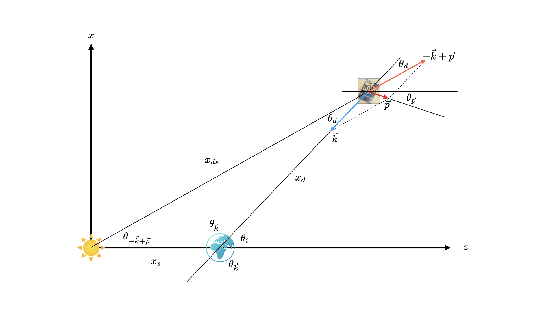
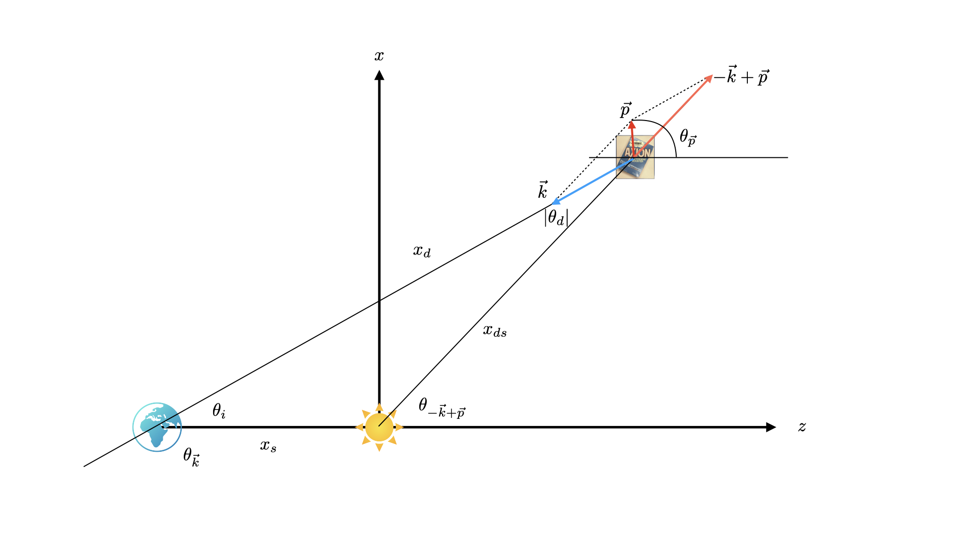
Let’s focus on a point source located at the origin of our coordinate system emitting radially and isotropically. We borrow part of our notation from Ref. [13]. We consider an ALP decay happening at a location $\vec{x}_{ds}$ that we choose to lie on the $xz$-plane. At $\vec{x}_{ds}$, the photons from the source have a unique direction

$$f_{\gamma}(\vec{q},\vec{x}_{ds}) = f_{\gamma}(\omega_{q},x_{ds})\frac{\delta(\theta_{\vec{q}}-\theta_{s})\delta(\phi_{\vec{q}})}{\sin\theta_{\vec{q}}}\enspace,$$ (2.2)

with $\theta_{s}$ determined by $\vec{x}_{ds}$. We take the Earth to lie on the $z$-axis. The geometry is shown in Figures 1 and 2. We consider two possible configurations: 1) the back-light echo coming from the direction opposite to the source, shown in Figure 1 and 2) the front-light echo coming from behind the source, shown in Figure 2.

For the axion phase space distribution, we choose a Maxwell-Boltzmann

$$f_{a}(\vec{p},\vec{x}\,)=n_{a}\frac{(2\pi)^{3}}{(2\pi)^{3/2}\delta p(\vec{x}\,)^{3}}\ e^{-\frac{(\vec{p}-\langle\vec{p}\,\rangle)^{2}}{2\delta p(\vec{x}\,)^{2}}}\enspace,$$ (2.3)

where $\langle\vec{p}\,\rangle$ is the average dark matter momentum in Earth’s rest frame and $\delta p(\vec{x}\,)$ is the momentum dispersion at a location $\vec{x}$. The axion number density is given by

$$n_{a}(\vec{x}\,)=\int\frac{d^{3}p}{(2\pi)^{3}}\,f_{a}(\vec{p}\,,\vec{x}\,)\enspace.$$ (2.4)

From Eq. (LABEL:boltzmann), with Eqs. (2.2) and (2.3), through the derivation described in Appendix A, we obtain

$$\frac{d\dot{n}_{a}}{d\omega_{k}d\Omega_{k}} = -n_{a}\,\frac{g^{2}m_{a}^{2}}{256\pi^{2}}\frac{N_{pol}}{2}\,f_{\gamma}(\omega_{k})\ h(\omega_{k},\vec{x}_{ds})\enspace,$$ (2.5)

with

$$h(\omega_{k},\vec{x}_{ds})=\frac{1}{(2\pi)^{3/2}\delta v^{3}}\ e^{-\frac{\langle v_{t}\rangle^{2}}{2\delta v^{2}}}\ e^{-\frac{(\varepsilon-\langle v_{\parallel}\rangle)^{2}}{2\delta v^{2}}}\ e^{-\frac{(\omega_{k}\theta_{d}/m_{a}-\langle v_{\perp}\rangle)^{2}}{2\delta v^{2}}}\enspace,$$ (2.6)

where we have used that for non-relativistic axions $\vec{p}=m_{a}\vec{v}$. In the equations above, $\Omega_{k}$ is the direction pointing from the decay location to the detector, $\langle v_{\parallel}\rangle$ and $\langle v_{\perp}\rangle$ are the components of the axion average velocity parallel and perpendicular to the line of sight (los) in the $xz$-plane, $\langle v_{t}\rangle$ is the average dark matter velocity perpendicular to the $xz$-plane, $\varepsilon=2\omega_{k}/m_{a}-1$, and $\theta_{d}$ is the angle between the los and the direction from the source to the decay location. In Eq. (2.5), $n_{a}$, $f_{\gamma}$, $\langle\vec{v}\,\rangle$ and $\theta_{d}$ are all functions of the decay location $\vec{x}_{ds}$. Explicit expressions for the components of $\langle\vec{v}\,\rangle$ are given in Appendix C.

The interpretation of Eq. (2.5) is the following. At the decay location $\vec{x}_{ds}$, the source’s photons arrive from a certain direction $\theta_{s}$. Any ALP present at $\vec{x}_{ds}$ can be stimulated to decay, but only if the ALP in question has velocity components $v_{\parallel}=\epsilon$, $v_{\perp}=\omega_{k}\theta_{d}/m_{a}$ and $v_{t}=0$ will the echo photon travel in the direction of Earth with frequency $\omega_{k}$. The likelihood of such a decay depends then on how many axion particles are available with the required momentum.

For a fixed observation angle $\theta_{i}\ll 1$, the deflection angle $\theta_{d}$ takes the following form

$$\theta_{d}=\pm\mathrm{arcsin}\left(\frac{x_{s}}{x_{ds}}\theta_{i}\right)\enspace,$$ (2.7)

where the upper sign corresponds to the back-light echo, the lower to the front-light echo. For the back-light echo, $x_{s}<x_{ds}$, so that a small $\theta_{i}$ implies a small $\theta_{d}$. For the front-light echo, instead, $x_{s}/x_{ds}$ can be large if the decay happens close to the source. Thus, in this case, a small $\theta_{i}$ does not necessarily imply a small $\theta_{d}$. However, for non-relativistic axions, decays with large $\theta_{d}$ are suppressed by the axion phase space distribution. So, in both cases, we can approximate

$$\theta_{d}=\pm\frac{x_{s}}{x_{ds}}\theta_{i}\enspace.$$ (2.8)

The decay rate is the largest at a frequency

$$\omega_{*}\approx\frac{m_{a}}{2}\left(1+\langle v_{\parallel}\rangle\right)\enspace,$$ (2.9)

and is suppressed exponentially for $\omega-\omega_{*}>m_{a}\delta v$. Since $\langle\vec{v}\,\rangle$ is small, we can approximate $\omega_{k}\sim m_{a}/2$ in Eq. (2.5), keeping corrections of order $\langle\vec{v}\,\rangle$ only in the exponents.

The rate of change of the axion number density can be related to the echo flux density observed from Earth. For each axion decay, two photons, each of energy $\sim m_{a}/2$ are produced. Only one of those travels toward Earth. The power emitted towards us per unit volume, unit frequency, and unit solid angle is then equal to $m_{a}/2\ |d\dot{n}_{a}/(d\nu_{k}d\Omega_{k})|$. Integrating along the los, we obtain the spectral intensity

$$I_{\nu}=\int dx_{d}\ \frac{m_{a}}{2}\Big{|}\frac{d\dot{n}_{a}}{d\nu_{k}d\Omega_{k}}\Big{|}\enspace,$$ (2.10)

where we assumed absorption effects to be negligible. Next, we need to relate the source’s photon phase space density to its flux density observed from Earth. Using Eq. (2.2), we obtain

$$f_{\gamma}(\omega,x_{ds})=\frac{(2\pi)^{3}}{N_{pol}\omega^{3}}\frac{d\rho_{\gamma}(x_{ds})}{d\omega}=\frac{(2\pi)^{3}}{N_{pol}\omega^{3}}\frac{d\rho_{\gamma}(x_{s})}{d\omega}\left(\frac{x_{s}}{x_{ds}}\right)^{2}\enspace,$$ (2.11)

where $\rho_{\gamma}$ is the photon energy density. The flux density through a surface area perpendicular to the direction Earth-source is $S^{(0)}_{\nu}(x_{s})=2\pi d\rho_{\gamma}(x_{s})/d\omega$.

Finally, from $S_{\nu}=\int d\Omega_{i}\,B(\Omega_{i})\int_{\rm los}dI_{\nu}$ we obtain

$$S_{\nu}=\frac{\pi g^{2}}{16m_{a}}\ S_{\nu}^{(0)}\int d\Omega_{i}\,B(\Omega_{i})\int dx_{d}\ \rho_{a}(\vec{x}_{ds})\,\left(\frac{x_{s}}{x_{ds}}\right)^{2}h(\omega_{k},\vec{x}_{ds})\enspace.$$ (2.12)

where $S_{\nu}^{(0)}$ is the source’s flux density as observed from Earth, $\Omega_{i}$ is the solid angle in the direction of the los $(\theta_{i},\leavevmode\nobreak\ \phi_{i})$, and $B$ describe the observing beam.

In Eq. (2.12), we have not taken into account two possible effects: the motion of the source with respect to Earth and the time dependence of the source’s luminosity. If we introduce these effects, Eq. (2.12) generalizes to

$$S_{\nu}(t)=\frac{\pi g^{2}}{16m_{a}}\ S^{(0)}_{\nu}(t)\int d\Omega_{i}\,B(\Omega_{i})\int dx_{d}\ \rho_{a}(\vec{x}_{ds})\,\frac{L_{\nu}(t_{em})}{L_{\nu}(t-\tilde{x}_{s}(t))}\left(\frac{\tilde{x}_{s}(t)}{\tilde{x}_{ds}(t_{em})}\right)^{2}h(\omega,\vec{x}_{ds},t_{em})\enspace,$$ (2.13)

where $\tilde{x}_{s}(t)$ is the distance from Earth to the actual position of the source at time $t$ (not to the position where the source appears to be), $\tilde{x}_{ds}(t)$ is the distance from the source to the decay location at time $t$, and $L_{\nu}$ is the luminosity of the source. At time $t_{em}=t-x_{d}-\tilde{x}_{ds}(t_{em})$, the source emitted a photon that subsequently traveled a distance $\tilde{x}_{ds}(t_{em})$ to the decay location, stimulated the decay of an ALP which in turn created a photon that traveled a distance $x_{d}$ to Earth, arriving at a time $t$. The time $t_{em}$ can be expressed as a function of $x_{d}$ and the velocity of the source $\vec{v}_{s}$ as described in Appendix B. The function $h$ is evaluated at a fixed location, determined by $\theta_{i}$ and $x_{d}$ independent of $t_{em}$, however, it develops a time dependence through $\theta_{d}$. This will become clear in Section 3.2.2.

3 Angular distribution of the echo on the sky

To study the angular distribution of the signal in the sky, we isolate from $S_{\nu}$ the following dimensionless quantity

$$g(\theta_{i},\phi_{i}) = x_{s}\int_{r_{min}}^{R}dx_{d}\ \frac{\rho_{a}(\vec{x}_{ds})}{\rho_{\odot}}\ \frac{L_{\nu}(t_{em})}{L_{\nu}(t-x_{s})}\ \frac{1}{x_{ds}(t_{em})^{2}}\ (2\pi)^{3/2}\delta v_{\odot}^{3}\ h(\omega,\vec{x}_{ds}(t_{em}))\enspace,$$ (3.1)

where $\rho_{\odot}$ and $\delta v_{\odot}$ are the dark matter density and velocity dispersion at the Sun’s location.

3.1 Idealized case

Figure 3: Angular distribution of the echo from decays happening at fixed distance $x_{d}$ in the idealized case. We set $\delta v=10^{-3}$.

As a first step, we want to establish a basis onto which to add the various effects relevant to the distribution on the sky of the echo intensity. To this end, we consider the academic case of an infinite dark matter halo with constant energy density $\rho_{a}(\vec{x}_{ds})=\rho_{\odot}$, velocity dispersion $\delta v(\vec{x}_{ds})=\delta v_{\odot}$, and null dark matter and source velocity $\langle\vec{v}\,\rangle=0$. We also assume constant source luminosity $L_{\nu}(t)$ and velocity $\vec{v}_{s}=0$. We fix the energy such that we are at resonance $\omega=\omega_{*}$. Under these assumptions, $g(\theta_{i},\phi_{i})$ reduces to

$$g_{id}(\theta_{i}) = x_{s}\int_{r_{min}}^{R}dx_{d}\ \frac{1}{x_{ds}^{2}}\ \ \exp\left(-\frac{\left(\frac{x_{s}}{x_{ds}}\theta_{i}\right)^{2}}{8\delta v^{2}}\right)\enspace.$$ (3.2)

A first observation is that, if in addition to requiring that the dark matter is at rest on average, we also require it to be perfectly cold, we obtain $g_{id}\propto\delta(\theta_{i})$. This is to be expected because, in the absence of average velocity and velocity dispersion, the echo travels back to the location where the source was when the photons that stimulated the decay were emitted. For a source at rest emitting radially, the only way to receive the echo radiation is to be between the source and the decay location.

When velocity dispersion is present, the intensity on a spherical shell of radius $x_{d}$ centered at Earth drops exponentially as $\theta_{i}$ increases beyond $\frac{x_{s}}{x_{ds}}\theta_{i}\gtrsim 2\delta v$. For fixed $x_{d}$, we thus have the typical size of the intensity patch

$$\theta_{i,0}\sim 2\delta v\left(\frac{x_{d}}{x_{s}}\pm 1\right)\enspace,$$ (3.3)

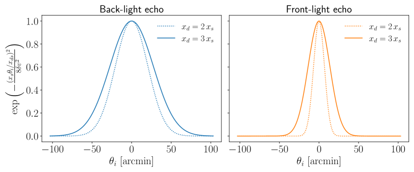
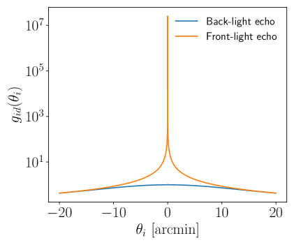
where we have approximated $x_{ds}=x_{d}\pm x_{s}$. Again, the upper sign holds for the back-light echo, the lower sign for the front-light echo. For given $x_{d}$, the intensity of the front-light echo is more compact than that of the back-light echo, because the distance to the source is smaller. We also notice that, for decays happening on shells of increasing $x_{d}$, the size of the patch becomes larger, as shown in Figure 3. Correspondingly, for fixed $\theta_{i}$, the back-light echo emission is peaked at $x_{d}=0$ if $\theta_{i}\lesssim 2\delta v$, while for larger observation angles $\theta_{i}>2\sqrt{2}\delta v$, the decay needs to happen at larger distances in order to have the same $\theta_{d}$. In this case, the largest contribution is from decays happening at $x_{d}=x_{s}(\theta_{i}/(2\sqrt{2}\delta v)-1)$ and the flux is suppressed by the distance. For the front-light echo, the flux from a given direction $\theta_{i}$ is always suppressed at distances $x_{d}<x_{s}(\theta_{i}/(2\sqrt{2}\delta v)+1)$. In both cases, the integrand decreases as $x_{d}^{-2}$ at large distances.

Figure 4: Emission profile of the echoes after integrating along the los in the idealized case. We set $\delta v=10^{-3}$.

Carrying on with our idealized case, we can integrate over $x_{d}$ analytically in the approximation $x_{ds}\approx x_{d}\pm x_{s}$. The lower integration limit is Earth’s radius for the back-light echo, while for the front-light echo we take $r_{min}=x_{s}$. Sending $R\to\infty$, the result is

$$g_{id}(\theta_{i}) = \frac{\sqrt{2\pi}\delta v}{\theta_{i}}\operatorname{erf}{\left(\frac{x_{s}\theta_{i}}{2\sqrt{2}\delta v(r_{min}\pm x_{s})}\right)}\enspace.$$ (3.4)

For the back-light echo, we can neglect $r_{min}$ compared to $x_{s}$. Eq. (3.4) reduces to

$$g_{id}^{(back)}(\theta_{i}) = \frac{\sqrt{2\pi}\delta v}{\theta_{i}}\operatorname{erf}{\left(\frac{\theta_{i}}{2\sqrt{2}\delta v}\right)}\enspace,$$ (3.5)

Notice that the result is finite for $\theta_{i}=0$

$$g_{id}^{(back)}(0) = 1\enspace.$$ (3.6)

For the front-light echo we can set the error function in Eq. (3.4) equal to 1, obtaining

$$g_{id}^{(front)}(\theta_{i}) = \frac{\sqrt{2\pi}\delta v}{|\theta_{i}|}\enspace.$$ (3.7)

The divergence at $\theta_{i}=0$ is only present in this hypothetical case, of an infinitely extended halo and an infinitely old source, since $R$ will be limited by the age of the source and the size of the Galaxy, once we introduce these effects. Moreover, the echo radiation from angles smaller than the radius of the source over $x_{s}$ is blocked by the source itself.

The idealized distribution on the sky is shown in Figure 4. The intensity is almost constant for $\theta_{i}\lesssim\delta v$ for the back-light echo, while for large $\theta_{i}$ it drops as $\theta_{i}^{-1}$. The typical size of the intensity patch on the sky is 10^′, taking $\delta v\sim 10^{-3}$. For the front-light echo, the intensity decreases as $\theta_{i}^{-1}$ everywhere.

Note also that the echo emission can be disentangled from the direct radiation from the source in the front-light echo case by using polarization. Indeed the echo polarization is orthogonal to the one of the source’s emission.

3.2 Realistic case

Source name	$l\leavevmode\nobreak\ (^{\circ})$	$b\leavevmode\nobreak\ (^{\circ})$	$x_{s}\leavevmode\nobreak\ (\mathrm{kpc})$	$\tau_{age}\leavevmode\nobreak\ (\mathrm{yrs})$	$l_{\vec{v}_{s}}\leavevmode\nobreak\ (^{\circ})$	$b_{\vec{v}_{s}}\leavevmode\nobreak\ (^{\circ})$
A	90	0	0.1	$5\times 10^{3}$	90	0
B	270	45	1	$10^{4}$	90	45
C	0	90	0.5	$5\times 10^{4}$	270	0
D	0	0.1	3	$10^{5}$	180	45

Table 1: Properties of hypothetical sources. The columns are the source galactic longitude $l$, galactic latitude $b$, distance from Earth as seen today $x_{s}$, age $\tau_{age}$ and direction of the source’s velocity in galactic coordinates $l_{\vec{v}_{s}}$ and $b_{\vec{v}_{s}}$. For all sources the magnitude of $\vec{v}_{s}$ is 200 km/s.

Now that we have identified the main features of the distribution on the sky of the echo intensity, we proceed to turn on one by one the effects coming from the characteristics of the dark matter halo and of the source.

Whenever an effect is not taken into consideration, the corresponding quantity in Eq. (3.1) is set to its default value. The default values are: $\rho(r)=\rho_{\odot}$, $x_{s}=0.1$ kpc, $\delta v(r)=\delta v_{\odot}$, $\langle v_{\perp}\,\rangle=0$, the age of the source $\tau_{age}=\infty$, $\vec{v}_{s}=0$ and $L=const$. In all plots of the next two subsections, we set the $\omega=\omega_{*}$ and we vary the observation angle $\theta_{i}$ leaving the galactic longitude of the los direction unchanged. Thus, when we talk about negative (positive) $\theta_{i}$, we mean that we are observing directions of lower (larger) galactic latitude than the source.

We illustrate the effects on four hypothetical sources with properties listed in Table 1.

3.2.1 Effects of the halo

Figure 5: Effects of the halo on the back-light echo.

Figure 6: Effects of the halo on the front-light echo.

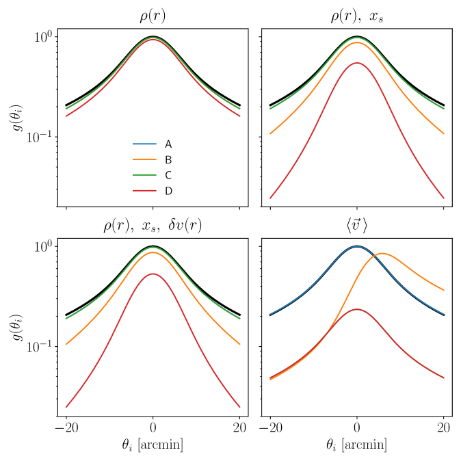
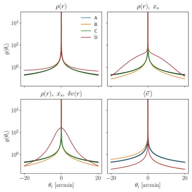
We consider a Navarro-Frenk-White halo, with parameters $\rho_{s}=0.41\leavevmode\nobreak\ \mathrm{GeV\leavevmode\nobreak\ cm}^{-3}$ and $r_{s}=20$ kpc [14], yielding a dark matter density at the Sun’s location $\rho_{\odot}=0.5\leavevmode\nobreak\ \mathrm{GeV\leavevmode\nobreak\ cm}^{-3}$. We calculate $\delta v(r)$ integrating the spherically symmetric Jeans equation assuming no velocity anisotropy (see for example Ref. [15]). We obtain $\delta v_{\odot}=144$ km/s.

We assume that the dark matter is on average at rest in a non-rotating frame attached to the Galaxy. Then the average velocity of dark matter in Earth’s rest frame $\langle\vec{v}\,\rangle$ is mainly given by $-\vec{v}_{\odot,\phi}$, where $\vec{v}_{\odot,\phi}$ is the velocity of the Sun in the tangential direction in the galactic plane with magnitude 245.6 km/s [16] in the direction of galactic coordinates $(l,b)=(90^{\circ},0^{\circ})$. We neglect the Sun’s velocity in the other directions as well as the motion of Earth with respect to the Sun.

We study the effect on the echo of the following quantities:

1. $\rho(r)$,

2. $\rho(r)$ in combination with the distance of the source $x_{s}$,

3. $\rho(r)$ in combination with $x_{s}$ and the velocity dispersion $\delta v(r)$,

4. the dark matter velocity relative to the Sun $\langle\vec{v}\,\rangle$.

In Figures 5 and 6, we show each of the effects above in a separate panel, for the back-light and front-light echo, respectively. The thick black line in all panels represents the idealized case $g_{id}(\theta_{i})$.

On the top left panel, we see the effect of the dark matter density profile. The lines for sources A, B, and C are on top of each other because the dark matter density along the los is the same in these three cases. We observe a minor suppression of the echo flux compared to the idealized case. On the other hand, for source D, the back-light echo flux is more significantly reduced because the los points away from the Galactic center. As expected, we see an increased flux for source D in the case of the front-light echo.

The top right panel shows the combined effect of the density profile and the distance to the source. Notice, that if we let $x_{s}$ vary among sources while keeping $\rho=\rho_{\odot}$ fixed, there would be no effect on the $g$ (see Eqs. (3.5), (3.7)). The lines for sources A and C are unchanged from the top left panel. For sourced B and D, whose distances are larger than the default value, we see a reduction of the flux for the back-light echo due to the lower dark matter density along the los. Conversely, for the front-light echo, we notice a substantial increase in flux for source D which is now placed closer to the Galactic center. This is due to the facts two facts: the dark matter density is higher where $x_{ds}\sim 0$, and the contribution from the high dark matter density at the Galactic center is not suppressed by a large value of $x_{ds}$.

The bottom left panel shows the effect of the variation of the velocity dispersion along the los in combination with the source distance and the variation of the dark matter energy density. In all cases, except for the front-light echo of source D, the effect is negligible. The velocity dispersion goes to zero at large galactic radii, causing a reduction of the echo flux from these locations. However, in this case, the flux is already suppressed by the distance and by the low dark matter density. We see instead a non-negligible effect on the front-light echo of source D, for which the los passes close to the Galactic center, where the velocity dispersion is small. For observation angles small enough to have $\theta_{d}<\delta v$ close to the Galactic center, we see an enhancement of the flux due to the normalization of $h(\omega,\vec{x}_{ds})$, i.e. there are more axions available to decay that will produce photons with the desired direction. If the observation angle is larger than that, the suppression from the exponential wins over the enhancement from the normalization factor and we observe a reduction of the flux.

The bottom right panel shows the effect of the average dark matter velocity. For source A, $\langle\vec{v}\,\rangle$ is almost completely along the los. Hence it does not affect the distribution of the echo on the sky, but rather it will shift its frequency. For source B, instead, we have a sizeable value of $\langle\vec{v}_{\perp}\rangle$. According to Eq.(2.6), the echo flux is the largest when $\omega_{k}\theta_{d}/m_{a}=\langle v_{\perp}\rangle$ or

$$\theta_{i}=\pm\frac{m\langle v_{\perp}\rangle}{\omega_{k}}\frac{x_{ds}}{x_{s}}$$ (3.8)

For the back-light echo, the emission is peaked at a location where $\theta_{i}$ has the same sign as $\langle v_{\perp}\rangle$. Now we have to be careful to interpret this correctly. From Eq. (A.12), we see that $\langle v_{\perp}\rangle$ has the opposite sign as $\langle v_{x}\rangle$ ($\cos\theta_{\vec{k}}<0$). Since $\theta_{i}$ grows in the positive $x$-direction, the peak of the back-light echo emission comes from the direction opposite to that of $\langle v_{x}\rangle$. In other words, the peak of the back-light echo emission is shifted in the direction opposite to that of the average dark matter velocity. When we look in the direction opposite to source B, the component of the average dark matter velocity perpendicular to the los points in the direction of decreasing galactic longitude, i.e. $\langle v_{x}\rangle<0$, causing the emission to peak at positive $\theta_{i}$. The contrary is true for the front-light echo, for which the largest emission comes from the direction where the dark matter velocity points. However, in this case, we don’t see a shift of the peak, but only an asymmetric distribution of the flux. For sources C and D, whose lines are on top of each other, we have $|\langle\vec{v}\,\rangle|\approx|\langle v_{t}\rangle|$, resulting in an overall reduction of the flux by a factor $\exp\left[-\langle v_{t}\rangle^{2}/2\delta v^{2}\right]$.

3.2.2 Effects of the source’s characteristics

Figure 7: Effects of the source characteristics on the back-light echo.

Figure 8: Effects of the source characteristics on the front-light echo.

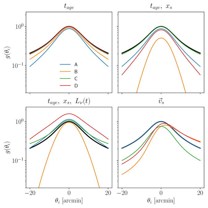
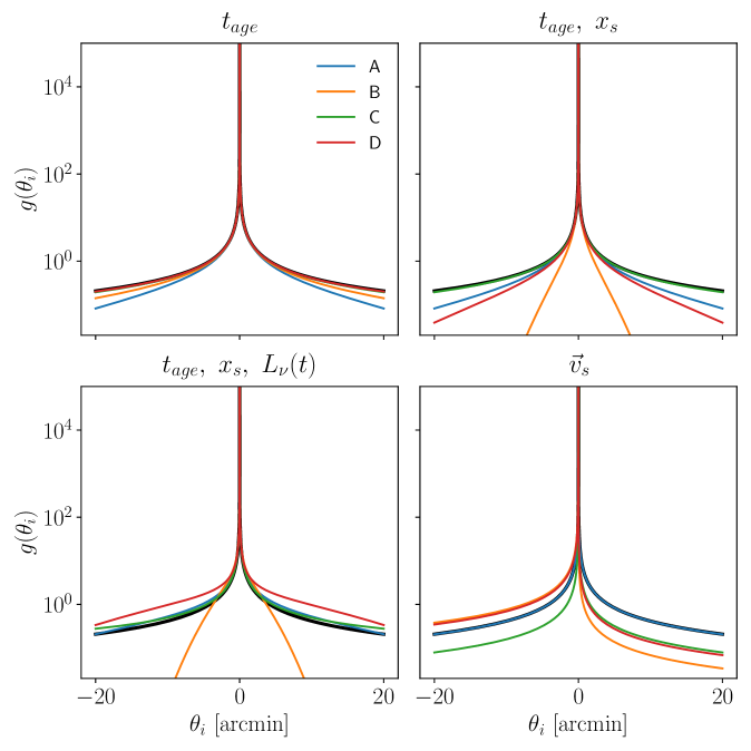
In this Section, we study how the properties of the source affect the echo emission. In particular, we take into account the following ones:

1. the age of the source $\tau_{age}$,

2. $\tau_{age}$ in combination with the distance of the source $x_{s}$,

3. $\tau_{age}$ in combination with the time dependence of the flux,

4. the motion of the source with respect to Earth.

Results are shown in Figures 7 and 8. The top left panel shows the effect of a finite a $\tau_{age}$. The age of the source translates into a reduced upper integration limit in Eq. (3.1). The time it takes a photon to travel the distance $x_{d}+x_{ds}$ cannot exceed $\tau_{age}$. The upper integration limit becomes then

$$R\sim\frac{1}{2}(\tau_{age}\mp x_{s})\enspace.$$ (3.9)

On the top left panel of Figures 7 and 8, we see the expected reduction of the flux for the younger sources. For the older sources, the upper integration limit cuts out locations from where the flux is already suppressed by a large value of $x_{ds}$, and the effect is negligible.

On the top right panel, we add a varying distance for the sources. For the back-light echo, a larger distance implies a reduced upper integration limit, resulting in a reduced flux from sources B and D compared to the top left panel. For the front-light echo, a large $x_{s}$ means a larger $R$, but also a larger $\theta_{d}$ for fixed $\theta_{i}$. For this reason, we see a dimming of the flux compared to the top left panel even if the upper integration limit is larger.

For the time dependence of the sources’ luminosity, we assume a power law

$$L_{\nu}(t)\propto\left(1+\frac{t}{\tau_{0}}\right)^{-\alpha}\enspace,$$ (3.10)

where $t$ is the time since the birth of the source. A positive $\alpha$ means that the source was brighter in the past. The bottom left panel shows how the flux increases for $\alpha=1$ and $\tau_{0}=10^{3}$ yr. As expected, the effect is larger for the older sources.

Finally, the bottom right panel shows the aberration effect due to the motion of the source. Assuming that the source moves with a constant velocity $\vec{v}_{s}$, its position at time $t$ is

$$\vec{r}_{s}(t)=(v_{s,x},\leavevmode\nobreak\ v_{s,x},\leavevmode\nobreak\ v_{s,z})\,(t+x_{s})\enspace,$$ (3.11)

where now $t=0$ is the time today. Let’s focus on a given decay location determined by the observation angle $\theta_{i}$ and the distance along the los $x_{d}$. The motion of the source deforms and rotates the triangle that has Earth, the source, and the decay location as vertices. From $\vec{v}_{s}$, we can obtain expressions for the time-dependent Earth-source distance $\tilde{x}_{s}(t)$, source-decay location distance $\tilde{x}_{ds}(t)$ and the direction from which the source’s photon reach the decay location $\theta_{s}(t)$, $\phi_{s}(t)$. Explicit expressions are given in Appendix B.

Let us first comment on the effect on the front-light echo shown in Fig. 8. We have chosen the velocity of the sources such that source A is moving towards us, meaning that it was further away in the past. In this case, the only effect is a mild increase in $x_{s}/x_{ds}$ and $\theta_{s}$ compared to the case of a source at rest. We find that this effect is negligible.

Source B is moving in the positive $x$-direction of Figure 2, meaning it was further down the $x$-axis in the past. If we start with a positive observation angle, at any time in the past the triangle was more open, because the angle between the los to the decay location and the los to the source was larger than today This leads to a suppression of the flux. On the other hand, if we start with $\theta_{i}<0$, the triangle closes as we go back in time, becoming a line when the source was along the los. This causes an increase in the flux.

To understand if this effect is important, we estimate at which distance along the los the decay must happen for us to be receiving today the echo radiation stimulated by photons emitted when the source was along the line of sight. The enhancement of the flux will be larger if the los crossing happened recently so that the decay location is close and well within the halo.

Setting $v_{s,y}=0$ we see from Figures 1 and 2, that the source was along the los when $\theta_{s}(t)=\theta_{i}$. Starting from a positive $\theta_{i}$, this happened at a time $t_{em}=\mp x_{s}\theta_{i}/v_{s,x}$, (see Eq. (B.2)) This tells us that the zero crossing of $\theta_{i}$ has occurred in the past for the front-light echo if $\theta_{i}$ and $v_{s,x}$ have opposite signs, the other way around for the back-light echo. The distance of the decay stimulated by photons emitted at $t_{em}$ is

$$x_{d}\sim\pm\frac{x_{s}}{2}\left(\frac{\theta_{i}}{v_{s,x}}-1\right)\enspace,$$ (3.12)

which may well be within the dark matter halo.

Going back to Figure 8, for source C, $\vec{v}_{s}$ is perpendicular to the plane $xz$-plane. This causes the triangle to open up, causing an overall reduction of the flux. Finally, source D is moving both away from us and in the positive $x$-direction. The result is similar to that of source B, the effect being reduced because of a smaller magnitude of $v_{s,x}$.

Let’s now turn to the back-light echo Fig. 7. For sources B and D, we see that in this case, the flux is larger for positive $\theta_{i}$. This is expected because now, due to the different geometry, the source crossed the los in the past if $\theta_{i}>0$.

4 Collinear emission

In this Section, we consider axion decays happening at locations between us and the source. In this case, the echo (with momentum $\vec{k}\,$) travels back toward the source, while the decay photons with the same momentum as the incoming ones (denoted by $\vec{q}\,$), travel toward us.

The Boltzmann equation now reads

$$\frac{d^{3}\dot{n}_{a}}{dq^{3}} = -\frac{1}{(2\pi)^{3}}\frac{1}{2\omega_{q}}\int\frac{d^{3}p}{(2\pi)^{3}}\frac{f_{a}(\vec{p}\,)}{2m_{a}}\ \frac{d^{3}k}{(2\pi)^{3}}\frac{1}{2\omega_{k}}(2\pi)^{4}\delta^{(4)}(k+q-p)\sum_{\lambda}|\mathcal{M}_{0}|^{2}(1+f_{\gamma}(\vec{q},\lambda))\enspace.$$

Following Appendix D, one obtains

$$\frac{d\dot{n}_{a}}{d\omega_{q}d\Omega_{q}} = -n_{a}\frac{g_{a\gamma}^{2}m_{a}^{2}}{64\pi^{2}}\,\frac{N_{pol}}{2}\,f_{\gamma}(\omega_{q})\delta(\Omega_{q})\ h_{col}(\omega_{q},\vec{x}_{ds})\enspace,$$ (4.2)

with

$$h_{col}(\omega_{q},\vec{x}_{ds})=\frac{1}{\sqrt{2\pi}\delta v}\ e^{-\frac{(\varepsilon-\langle v_{\parallel}\rangle)^{2}}{2\delta v^{2}}}\enspace.$$ (4.3)

The decay rate is the largest for $\varepsilon=\langle v_{\parallel}\rangle$, where, as before, $\langle v_{\parallel}\rangle$ is the average axion velocity along the direction of the momentum of the photon coming towards us, $\vec{q}$.

Here $\Omega_{q}$ is the angle between the direction of the stimulating photon and the direction of the photon emitted in the ALP decay. The delta-function $\delta(\Omega_{q})$ indicates that the collinear emission comes exactly from the direction of the source, and is not smeared over the sky by the axion momentum dispersion as it happens instead for the echo case.

Proceeding like in Section 2, we obtain the flux density

$$S_{\nu}=\frac{\pi g^{2}}{4m}\ S_{\nu}^{(0)}\int d\Omega_{i}\,B(\Omega_{i})\int dx_{d}\,\delta(\Omega_{q})\,\rho_{a}(\vec{x}_{ds})\,\left(\frac{x_{s}}{x_{ds}}\right)^{2}\,h_{col}(\omega_{q},\vec{x}_{ds})\enspace.$$ (4.4)

With simple geometrical considerations, one can see that, in the limit of small angles, $\theta_{q}=\theta_{i}\,(x_{d}+x_{ds})/x_{ds}$, from which it follows $\delta(\Omega_{q})=\delta(\Omega_{i})\,x_{ds}^{2}/x_{s}^{2}$. We can thus recast Eq. (4.4) in a simpler form:

$$S_{\nu}(t)=\frac{\pi g^{2}}{4m}\ S_{\nu}^{(0)}(t)\,\int dx_{ds}\ \rho_{a}(\vec{x}_{ds})\,h_{col}(\omega_{q},\vec{x}_{ds})\enspace.$$ (4.5)

where, in analogy to Section 2, we also generalized the equation to include the time dependence of the source’s flux.

Compared to Eq. (2.13), the factor $L_{\nu}(t_{em})/L_{\nu}(t-\tilde{x}_{s}(t))$ is not present, because the photons produced in the decay travel together with the ones coming directly from the source, i.e. $t_{em}=t-\tilde{x}_{s}(t)$. Note that in the collinear case, if the source is time-dependent on short timescales, e.g., it has pulsations, the same time-dependency occurs also for the echo signal.

The motion of the source also enters, in principle, through a time-dependent $\delta(\Omega_{i})$. However, as long as the source doesn’t move out of the beam during the course of one observation, the proper motion of the source is completely negligible.

5 Forecast for pulsars

Now, we apply the formalism we developed in the previous Sections to the case of Galactic pulsars as stimulating source. Pulsars in connection to ALPs were considered in [17], but looking at a signal different from the one considered in our work. Ref. [17] studied the ALP conversion in the pulsar magnetic field. Here we derive prospects for detecting the echoes and collinear emission described above.

Our formalism applies to point sources emitting isotropically. The radio emission of pulsars is however not isotropic, but rather concentrated into a rotating beam confined within the polar cap region. The typical opening angle of the beam is [18]

$$\rho\sim 5.4^{\circ}\left(\frac{P}{\rm s}\right)^{-1/2}\enspace.$$ (5.1)

Since the echo intensity is spread over angular distances of order tens of arcminutes, and barring complications due to possible changes of direction of the pulsar’s rotation axis or magnetic field lines, we can safely consider the time-averaged pulsar emission to be isotropic in the directions that are relevant to us. A complication may arise due to the pulsar’s proper motion. If the source was further away from the line of sight in the past, it may be the case that the angle $\theta_{s}(t)$ was larger than $\rho$. In the following, we remove from our integration over the line-of-sight locations for which this is the case. We find that this effect is completely negligible.

Since the flux density involves the product $S^{(0)}_{\nu}\,x_{s}\,g(\Omega_{i})$, we focus on the pulsars with the largest flux times distance product in the ATNF catalog [19] and then take into account all the effects described in the previous Section.

Most of the relevant information is available directly from the ATNF catalog, with the exception of the source’s velocity along the line of sight and the time dependence of the source luminosity. From the analysis of Section 3.2.2, we know that the velocity along the los only affects the flux in a negligible way. We thus set it to zero. The time dependence of the flux luminosity is discussed in the next Subsection.

5.1 Modeling of the time dependence of the pulsar flux

The flux from a pulsar typically varies on timescales of order 1 second because of the pulsar’s rotation. However, as already noted in [13], this time dependence is not present in the echo flux. In fact, the echo is the aggregate of photons produced in decays that happened at different distances along the los. At these locations, the flux from the source peaks at different times, due to the different travel times from the source location. Since we integrate in Eq. (2.13) over distances of order the size of the halo, the travel time is much longer than the pulsar period and thus we expect the echo flux to be constant in time. Thus, in the following, we consider the pulsar’s luminosity averaged over timescales much larger than its period, but much smaller than its age. On the other hand, the time dependence of collinear emission is exactly the same as that of the source’s emission.

Pulsars are the brightest at their birth, their luminosity decreasing in time following the spin-down power $\dot{E}$. For the time-dependent evolution of the spin-down power, we consider the following equation, from the spin-down evolution in the magnetic dipole model (braking index $n=3$) [20]

$$\dot{E}(t)=\dot{E_{0}}\left(1+\frac{t}{\tau_{0}}\right)^{\beta}\enspace,$$ (5.2)

with $\beta=-2$. The constant $\tau_{0}$ is given by

$$\tau_{0}=\frac{P_{0}}{2\dot{P_{0}}}\enspace,$$ (5.3)

where $P_{0}$ and $\dot{P_{0}}$ are the initial spin and spin derivative of the pulsar. It is very challenging to infer the initial $P_{0}$ and $\dot{P_{0}}$ distributions. For example, given $P$ and $\dot{P}$ today, it is not possible to determine $P_{0}$ unless an independent measure of the pulsar’s age is available [18].

The authors Ref. [21] analyzed a population of young neutron starts associated with supernova remnants, for which it is possible to estimate the actual age of the pulsar. They found a log-normal distribution for the initial period, with mean $\log_{10}(P_{0}/\rm s)=-1.04^{+0.15}_{-0.2}$ and standard deviation is $\sigma_{P_{0}}=0.53^{+0.12}_{-0.08}$. In the dipole model, the magnetic field is constant, since it depends only on the product $P\dot{P}$, so that we can assume that the initial magnetic field distribution corresponds to the present one. From [21], the present B-field distribution is best-fitted by a log-normal with mean $\log_{10}(B/\rm G)=12.44$ and standard deviation $\sigma_{B}=0.44$. We use the mean values of these distributions as benchmarks to evaluate the impact of the pulsar spin-down temporal evolution

Using the mean values of the initial spin and magnetic field distributions in expression for the characteristic magnetic field [18]

$$B=3.2\times 10^{19}\leavevmode\nobreak\ \mathrm{G}\leavevmode\nobreak\ \sqrt{\frac{P}{\mathrm{s}}\dot{P}}\enspace,$$ (5.4)

we obtain $\tau_{0}=1.79\times 10^{4}$ yr.

The next ingredient is the relation between the spin-down power and the pulsar’s luminosity at a given frequency. Recently, Ref. [22] presented the largest, uniform, census of young pulsars deriving for 1170 objects correlation between the radio (pseudo)luminosity and parameters such as age and spin-down power. They found that, in the L-band, $\log L_{L}=c_{\dot{E}}\log\dot{E}$ with $c_{\dot{E}}=0.15\pm 0.02$. Assuming $c_{\dot{E}}$ to be independent, we obtain that the luminosity of a pulsar follows Eq. (3.10) with exponent $\alpha=0.3$.

We find that with this value of $\tau_{0}$ and $c_{\dot{E}}$ the effect on the echo of time dependence of the source’s flux is negligible. We thus neglect this effect in our forecasts. In doing this we are being conservative, since, for example, the actual value of $\tau_{0}$ for a given pulsar may very well be smaller than our benchmark value.

5.2 Target selection

Figure 9: Bandwidth-averaged front-light echo spectral intensity at 400 MHz for four of the most promising pulsars from the ATNF catalog assuming $g_{a\gamma}=10^{-11}\leavevmode\nobreak\ \mathrm{GeV}^{-1}$. Blue arrows indicate the direction of the component of the average dark matter velocity perpendicular to the line of sight, while magenta arrows indicate the source’s proper motion. The arrows are drawn in arbitrary units, but their relative lengths are to scale with each other. The thin black lines mark contours of constant $\langle I_{\nu}\rangle$.

Figure 10: Bandwidth-averaged front-light echo spectral intensity at 400 MHz for four of the same pulsars as Figure 9 assuming $g_{a\gamma}=10^{-11}\leavevmode\nobreak\ \mathrm{GeV}^{-1}$. On the left (right) panel, we vary the galactic latitude (longitude) of the line of sight, keeping the galactic longitude (latitude) fixed.

To estimate our projected sensitivity, we choose to integrate over the bandwidth that maximizes the signal-to-noise ratio. Assuming noise scales like $\sqrt{\Delta\nu}$, a top-hat bandwidth and $\nu=m_{a}(1+\langle v_{\parallel}\rangle)/4\pi$, we find that the optimal bandwidth is $\Delta\nu/\nu=2.8\delta v$ [12].

For the targets we are considering, the effect on the echo of a position-dependent velocity dispersion is negligible. We fix then $\Delta\nu$ based on the velocity dispersion at Earth. The frequency-averaged echo spectral intensity is

$$\langle I_{\nu}\rangle=f_{\Delta\nu}\,\frac{g_{a\gamma}^{2}}{16\Delta\nu}\ S_{\nu}^{(0)}\int dx_{d}\ \rho_{a}(\vec{x}_{ds})\,\left(\frac{x_{s}}{x_{ds}}\right)^{2}h_{1}(\omega_{k},\vec{x}_{ds})\enspace,$$ (5.5)

with

$$h_{1}(\vec{x}_{ds})=\frac{1}{8\pi\delta v^{2}}\ e^{-\frac{\langle v_{t}\rangle^{2}}{2\delta v^{2}}}\ e^{-\frac{(\theta_{d}/2-\langle v_{\perp}\rangle)^{2}}{2\delta v^{2}}}\enspace,$$ (5.6)

where we have neglected terms of order $\theta_{d}^{2}$ or $v\theta_{d}$. The Gaussian integrated over the chosen bandwidth provides $f_{\Delta\nu}=0.84$. The frequency-averaged flux density can be then obtained from the usual $\langle S_{\nu}\rangle=\int d\Omega_{i}\,B(\Omega_{i})\int_{\rm los}d\langle I_{\nu}\rangle$.

Similarly, for the collinear emission we have

$$\langle S_{\nu}\rangle=f_{\Delta\nu}\frac{g_{a\gamma}^{2}}{16\Delta\nu}\ S_{\nu}^{(0)}\int dx_{d}\ \rho_{a}(x_{d})\enspace.$$ (5.7)

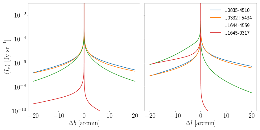
In Figure 9, we show the bandwidth-averaged echo spectral intensity at a frequency of 400 MHz for the four pulsars in the ATNF catalog with the largest product of distance times flux. We assume an axion photon coupling $g_{a\gamma}=10^{-11}\leavevmode\nobreak\ \mathrm{GeV}^{-1}$. We take the flux from the best fit to observations from the recent catalog of [23]. We note that the flux at 400 MHz is slightly lower than the one reported in ATNF. In Figure 10, we show slices of constant galactic longitude and latitude to ease the comparison among pulsars.

All effects discussed in Section 3.2 are implemented with the exception of the time dependence of the source’s luminosity. We have set $v_{s,z}=0$, as this quantity is not known and we have established it is not important for the echo. The age of the pulsar used to determine the upper limit of integration is taken to be the characteristic age $\tau_{age}$ plus the pulsar distance.

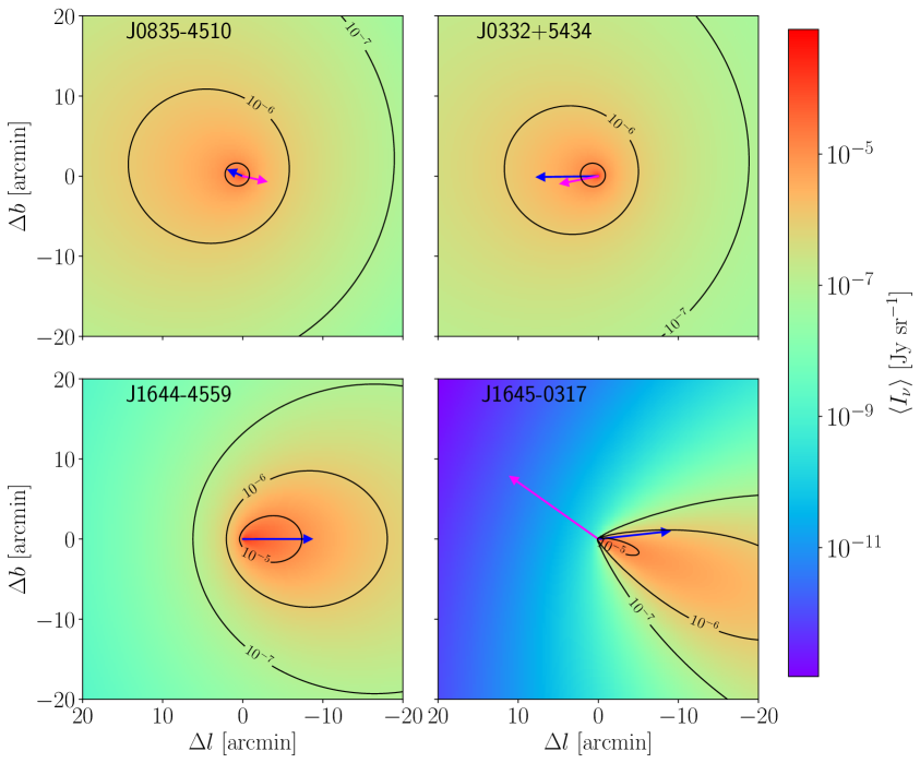
The Vela pulsar J0835-4510 is the brightest source at this frequency with a flux of about 5 Jy. Its front-light echo flux does not experience significant reduction due to any of the effects discussed in Section 3.2. There is some dimming compared to the idealized case due to the young age $\tau_{age}=1.13\times 10^{4}$ yr, and, to a lesser extent, to the dark matter density along the line of sight. The dark matter velocity is essentially along the los, thus affecting the resonance frequency, but not the distribution of the echo on the sky. The projection on the sky of $\langle\vec{v}\rangle$ is shown by the blue arrow in Fig 9. The small velocity of the source, $\vec{v}_{s}\sim 60$ km/s, shown by the magenta arrow, makes the intensity larger for positive values of $\Delta l$, as also visible on the right panel of Fig. 10.

Pulsar J0332+5434 has the largest $x_{s}\,S_{\nu}^{(0)}$, a factor 1.8 larger than Vela. However, its galactic longitude $l=144^{\circ}$, and distance $x_{s}=1.695$ kpc, imply that the average dark matter density along the los is low making it lose its ‘advantage’. The average dark matter and source velocities point approximately in the same direction. From the discussion of Section 3.2.1, we know that for the front-light echo, the intensity is larger in the direction of $\langle\vec{v}\rangle$, while in Section 3.2.2 we have learned that the intensity is larger in the direction of $-\vec{v}_{s}$ (where the source was in the past). For J0332+5434 the two effects tend to compensate, resulting in an intensity patch similar to that of Vela.

Next, we have J1644-4559 and J1645-0317. These two pulsars have similar fluxes at 400 MHz of about 0.4 Jy and comparable distances of order 4 kpc. Their galactic coordinates are $(339^{\circ},\leavevmode\nobreak\ -0.195^{\circ})$ and $(14.1^{\circ},\leavevmode\nobreak\ 26.1^{\circ})$, respectively, implying that the dark matter density along both lines of sight is comparable, as well as the projection of the dark matter velocity on the sky. The main difference between the two is due to our description of their proper motion. For J1644-4559, proper motion information is not available and we set its velocity to zero. J1645-0317 on the other hand has a large velocity of about 375 km/s which causes a drastic reduction in the flux in the direction of $\vec{v}_{s}$.

5.3 Observational prospects

Figure 11: Projected sensitivity on the ALP-photon coupling $g_{a\gamma}$ versus ALP mass $m_{a}$, for different scenarios, described in Section 5.3. The upper colored cases corresponds to observations of single pulsars with either SKA-1 or LOFAR 2.0. More precisely, we show the cases of J0835-4510 (blue), J1644-4559 (green), J1645-0317 (red), and J0332+5434 (orange), including both the front-light echo signal (dashed) and collinear emission (solid). The two black curves report the sensitivity for surveys of all Galactic pulsars with SKA-1 (dashed) and SKA-2 (solid) considering only the collinear case.

For our forecasts, we consider two interferometric observatories of the near future: SKAO for the Southern hemisphere and LOFAR 2.0 for the Northern hemisphere.

Concerning the performance of the first phase of the SKA project, which used to be referred to as SKA-1, we follow [24], see their Tables 6 and 7. For example, at 114 MHz, the sensitivity of SKA-1 Low is $\sigma\sim 184\,\mu{\rm Jy}/{\rm beam}\,\sqrt{100\,{\rm hr}/\Delta t}\,\,\sqrt{10^{-4}/(\Delta\nu/\nu)}$ for a beam of size between $12^{\prime\prime}$ and $10.2^{\prime}$, while for SKA-1 Mid at 1.05 GHz, the sensitivity is $\sigma\sim 18.6\,\mu{\rm Jy}/{\rm beam}\,\sqrt{100\,{\rm hr}/\Delta t}\,\,\sqrt{10^{-4}/(\Delta\nu/\nu)}$ for a beam of size between $0.8^{\prime\prime}$ and $1.8^{\prime}$. SKA-1 should become operative in its final configuration in 2029.

A further development of the SKAO, which used to be referred to as SKA-2, is foreseen for the 2030’s, with telescope specifications still to be decided. According to [25], the goal is to reach a factor of $\times 10$ improvement in sensitivity with respect to SKA-1.

For very low-frequency emission and/or Northern hemisphere targets, we consider LOFAR 2.0, which is an ongoing program including a set of upgrades of the LOFAR stations and an increase of the capabilities of the array, expected to be completed in 2024. We consider the foreseen sensitivity reported in [26]. At 150 MHz, it is $\sigma\sim 200\,\mu{\rm Jy}/{\rm beam}\,\sqrt{100\,{\rm hr}/\Delta t}\,\,\sqrt{10^{-3}/(\Delta\nu/\nu)}$ for a beam at arcsec resolution.

In this Section, we will derive forecasts for the front-light echo and collinear emission. For both of them, we can use the point-like source sensitivity of the telescopes. Bounds are derived requiring $\langle S_{\nu}\rangle<2\sigma_{rms}$, and assuming that the background continuum emission in a single frequency channel can be subtracted away by fitting its shape in the full bandwidth. In the collinear case, we consider an improvement in the sensitivity by a factor $\sqrt{W/(P-W)}$, where $W$ is the width of the pulsation and $P$ is the period.

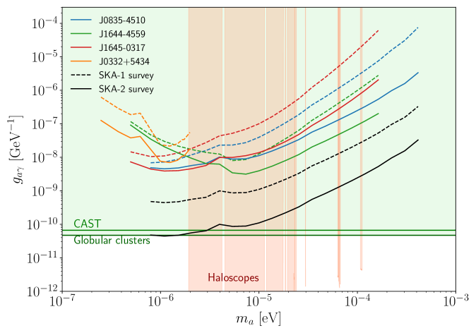
The first case shown in Fig. 11 concerns the sensitivity forecast for 100 hr observations of single pulsars (colored curves). We consider the same four pulsars described in Section 5.2. The pulsars J0835-4510, J1644-4559, and J1645-0317 are in the Southern hemisphere, under the SKA-1 reach. For the observation of J0332+5434 in the Northern hemisphere we instead use LOFAR 2.0. In the case of the front-light echo (color dashed), we remove the contribution from observation angles smaller than the frequency-dependent size of the broadened pulsar image. This would be given by photons passing again through the pulsar, where they might be absorbed or rescattered. For simplicity, we discard those photons. The pulsar’s apparent angular size is given by the broadening due to the scattering of photons in the interstellar medium and it is related to the scattering timescale $\tau_{s}$ as $\theta_{b}=\sqrt{\tau_{s}/x_{s}}$ [18].

As it can be seen from Fig. 11, in this case, prospects fall into a strongly constrained region of the ALP parameter space.

On top of the forecast for a single pulsar, we then estimate the projected sensitivity in the case of a survey of all Galactic pulsars. Such survey is planned for SKAO [27] with an already ongoing program along this direction conducted with MeerKAT [28]. Providing an accurate sensitivity forecast for the survey case is beyond the goal of this paper since it would require knowing the schedule of observations and performing simulations of pulsar populations. We can however derive a simple but reliable projected sensitivity in the following way. Let’s assume Vela (J0835-4510) to be a typical pulsar, in terms of luminosity and other properties, and to be the closest one, which also means the brightest one in terms of flux. We consider a radio luminosity distribution $N\propto L^{-0.8}$ for Galactic pulsars, as found in [29]. Let us now take a conservative simple 1D distribution along the direction to the Galactic center, or, say in other words, let us conservatively assume $N\propto S^{(0)-0.8}_{\nu}$ (in reality it will be somewhat steeper). This implies that the collective pulsar flux measured in a survey is $\int dS\,S\,dN/dS\simeq 4\,S^{(0)}_{\rm Vela}$. Then we take an average pulsar distance of $\langle d\rangle\simeq 8$ kpc and an average DM density between us and the pulsar of $\simeq 2.9\,\rho_{\odot}$, obtained volume averaging the NFW profile used in Section 3 above in the inner 8 kpc from the Galactic center. Finally, we assume 10 hr of observations for each survey field (which, in general, will contain several pulsars), instead of 100 hr considered for the single pulsar case discussed above. Combining all these arguments we obtain an improvement of a factor of $\sim 10.2$ in the projected $g_{a\gamma}$ bound with respect to the case considering the Vela pulsar only.

In Fig. 11, we show the forecast for a survey with SKA-1 assuming this simple rescaling factor (black dashed). We focus on the collinear signal since we saw from the single pulsar case that it is more promising than the front-light echo.

Our ultimate forecast is for a survey with SKA-2 (black solid). It has the capability to reach the allowed region of the ALP parameter space for $\mu$eV masses.

6 Conclusions

In this work, we derived the formalism for computing the signal associated with photon emission from the stimulated decay of axions. We started from first principles and focused on the stimulating point-like sources from our Galaxy. The presence of $\mu$eV ALPs in the Milky Way halo would imply the existence of three distinct line signatures:

1. Front-light echo: Stationary emission from approximately the same direction of the stimulating source and with a slightly broadened size and an orthogonal polarization.

2. Back-light echo: Stationary emission from the opposite direction with respect to the stimulating source and with a significantly broadened size and an orthogonal polarization.

3. Collinear emission: Possibly pulsed emission (if the stimulating source is pulsed) with the same direction, size, and polarization of the stimulating source.

It is difficult to imagine an astrophysical source providing simultaneously all these three line signatures with the above properties. Therefore, they offer a unique opportunity for a clear ALP identification.

Previous works [5, 6, 7, 8, 9, 10, 11, 12, 13] have discussed similar or connected signals, and here we aim at providing a comprehensive view.

We discussed how the echoes and the collinear emission depend on the ALP DM properties, namely on the DM spatial and velocity distributions, and on the source characteristics, such as distance, age, and motion. These dependencies offer extra handles for the ALP signal identification.

In the final part of the paper, we focused on the case of Galactic pulsars as stimulating sources. We showed that pulsar radio surveys of the next decade can be used to identify the described signatures for $\mu$eV ALPs.

Note added: Once this work was in its final phase, Ref. [30] appeared on arXiv. They discuss the two echoes (called gegenschein) and the collinear emission (called forwardschein), focusing on the observational prospects associated with supernova remnants. Our work aims instead at providing a detailed and general derivation of the effects.

Appendix A Derivation of the decay rate

In this Section, we derive the number of ALP decays per unit time and unit volume that produce photons of a given frequency $\omega_{k}$ traveling in a given direction $\Omega_{k}$, given the position of a point-like stimulating source that emits radially and isotropically. The number of decays can be related to the echo flux density at Earth as described in Section 2.

Our starting point is the Boltzmann equation Eq. (LABEL:boltzmann). Throughout the following derivation, we assume ALPs are non-relativistic. We keep corrections in the ALP momentum $\vec{p}$ only up to linear order, and only when they are relevant to the echo’s frequency or direction. Namely, when the correction only affects the magnitude of the decay rate, we ignore it.

Using the delta-function to eliminate the integral over $\vec{q}$ in Eq. (LABEL:boltzmann), we obtain

$$\frac{d^{3}\dot{n}_{a}}{dk^{3}} = -\frac{1}{(2\pi)^{3}}\frac{1}{(2\omega_{k})^{2}}\int\frac{d^{3}p}{(2\pi)^{3}}\frac{f_{a}(\vec{p}\,)}{2m_{a}}\ (2\pi)\delta(\omega_{q}+\omega_{k}-m_{a})\sum_{\lambda}|\mathcal{M}_{0}|^{2}(1+f_{\gamma}(\vec{q},\lambda))\Big{|}_{\vec{q}=-\vec{k}+\vec{p}}\enspace.$$

The matrix element is

$$\sum_{\lambda}|\mathcal{M}_{0}|^{2}=g_{a\gamma}\,|\epsilon^{\mu\nu\rho\sigma}(\hat{e}^{(1)}_{\mu}\hat{e}^{(2)}_{\nu})^{*}k_{1,\rho}k_{2,\sigma}|=g_{a\gamma}^{2}\frac{m_{a}^{4}}{2}\frac{N_{pol}}{2}\enspace,$$ (A.2)

where we allow the possibility for the source to be polarized. The frequency of the incoming photon can be expanded as

$$\omega_{q}\sim\omega_{k}-p\cos\psi\enspace,$$ (A.3)

where $\psi$ is the angle between $\vec{k}$ and $\vec{p}$. From the energy-conserving delta function, we see that the frequency of the echo photons must be close to half the ALP mass, shifted by a small amount proportional to the ALP velocity along the direction of $\vec{k}$

$$\omega_{k}=\frac{m_{a}+p\cos\psi}{2}\enspace.$$ (A.4)

We choose the coordinate system of Figures 1 and 2 and focus on a point source emitting radially and isotropically by using Eq. (2.2). Keeping in mind that $f_{\gamma}$, $f_{a}$, and thus $d^{3}\dot{n}_{a}/dk^{3}$ depend on the decay location $\vec{x}_{ds}$, we can write

$$\frac{d^{3}\dot{n}_{a}}{dk^{3}} = -\frac{g_{a\gamma}^{2}m_{a}}{4}\frac{N_{pol}}{2}\,f_{\gamma}\left(\frac{m_{a}}{2}\right)\frac{1}{(2\pi)^{5}}\ I(\vec{k}\,)\enspace,$$ (A.5)

with

$$I(\vec{k}\,) = \int d^{3}p\ f_{a}(\vec{p}\,)\ \delta(\omega_{q}+\omega_{k}-m_{a})\frac{\delta(\theta_{q}-\theta_{s})\delta(\phi_{\vec{q}})}{\sin\theta_{\vec{q}}}\Big{|}_{\vec{q}=-\vec{k}+\vec{p}}\enspace,$$ (A.6)

To eliminate the integrals over the axion phase space, we need to relate the angles of $\vec{q}$ to those of $\vec{p}$. We choose the decay location to be positioned in the first quadrant on the $xz$-plane. Then the momentum of the echo photon must have an azimuthal angle $\phi_{\vec{k}}=\pi$. Requiring that $\phi_{\vec{q}}=0$ then yields $\phi_{\vec{p}}=0,\pi$. Solving $\vec{p}=\vec{k}+\vec{q}$, we get

$$p = \sqrt{\omega_{k}^{2}+\omega_{q}^{2}+2\omega_{k}\omega_{q}\cos(\theta_{\vec{k}}+\theta_{\vec{q}})}$$

$$\theta_{p} = \begin{cases}-\arctan\left(\frac{\omega_{k}\cos\theta_{\vec{k}}+\omega_{q}\cos\theta_{\vec{q}}}{\omega_{k}\sin\theta_{k}-\omega_{q}\sin\theta_{\vec{q}}}\right),&\text{if $\phi_{p}=0$}\\ \arctan\left(\frac{\omega_{k}\cos\theta_{\vec{k}}+\omega_{q}\cos\theta_{\vec{q}}}{\omega_{k}\sin\theta_{k}-\omega_{q}\sin\theta_{\vec{q}}}\right),&\text{if $\phi_{p}=\pi$}\\ \end{cases}$$ (A.7)

We can now perform the change of variable $d^{3}p\to d^{3}q$ in Eq. (A.6)

$$I(\vec{k}\,) = \omega_{k}^{2}\int d\omega_{q}\,d\theta_{q}\,d\phi_{q}\ f_{a}(\vec{p}\,)\ \delta(\omega_{k}+\omega_{q}-m)\delta(\theta_{\vec{q}}-\theta_{s})\delta(\phi_{\vec{q}})\Big{|}_{\vec{p}=\vec{p}(\vec{q}\,)}$$ (A.8)

$$= \omega_{k}^{2}\ f_{a}(\vec{p}\,(\vec{q}\,))\ \Big{|}_{\begin{subarray}{c}\omega_{q}=m-\omega_{k}\\ \theta_{\vec{q}}=\theta_{s}\end{subarray}}\enspace.$$

The equation above tells us that, for a fixed direction of stimulating photons arriving at the decay location, given by $\theta_{s}$, an ALP with a specific momentum needs to be involved in the decay in order for the echo to have momentum $\vec{k}$ and to reach Earth. In the coordinate system of Figures 1 and 2, the components of the axion momentum involved in such a decay are

$$p_{x} = -\omega_{k}\sin\theta_{\vec{k}}+(m-\omega_{k})\sin\theta_{s}$$

$$p_{y} = 0$$

$$p_{z} = \omega_{k}\cos\theta_{k}+(m-\omega_{k})\cos\theta_{s}\enspace.$$ (A.9)

It is convenient to express $\theta_{s}$ in terms of the angle between the direction of the photons from the source coming into the decay location and the direction of the echo photons traveling towards Earth

$$\theta_{d}=\pi-\theta_{\vec{k}}-\theta_{s}\enspace.$$ (A.10)

One can check that $\theta_{d}$ is of order the axion velocity. More precisely, to linear order in $p$

$$\theta_{d} = \frac{p}{\omega_{k}}\sin(\theta_{\vec{k}}\pm\theta_{\vec{p}})\enspace.$$ (A.11)

We can then expand Eqs (A.9) to first order in the small quantities $\theta_{d}$ and $\epsilon=2\omega_{k}-m$, obtaining

$$p_{x} = \omega_{k}\theta_{d}\ \cos\theta_{k}-\epsilon\sin\theta_{k}$$

$$p_{z} = \epsilon\ \cos\theta_{k}+\omega_{k}\theta_{d}\ \sin\theta_{k}\enspace.$$ (A.12)

Let’s define components of the axion momentum parallel and perpendicular to $\vec{k}$, through the following rotation

$$\left(\begin{array}[]{cc}p_{\perp}\\ p_{\parallel}\\ \end{array}\right)=\left(\begin{array}[]{cc}\cos\theta_{k}&\sin\theta_{k}\\ -\sin\theta_{k}&\cos\theta_{k}\\ \end{array}\right)\left(\begin{array}[]{cc}p_{x}\\ p_{z}\\ \end{array}\right)=\left(\begin{array}[]{cc}\omega_{k}\theta_{d}\\ \epsilon\\ \end{array}\right)\enspace.$$ (A.13)

The axion momentum $\vec{p}\,$ necessary to produce an echo photon with frequency $\omega_{k}$ and direction $\theta_{k}$, given the direction of the incoming photon $\theta_{s}$, has a component along the direction of $\vec{k}$ equal to $\epsilon$, and the component perpendicular to $\vec{k}$ equal to $\omega_{k}\theta_{d}$.

Inserting our expression for $\vec{p}$ into Eq. (2.3), we obtain the desired result

$$I(\vec{k}\,) = n_{a}\,\left(\frac{m_{a}}{2}\right)^{2}\frac{(2\pi)^{3}}{(2\pi)^{3/2}\delta p^{3}}\ e^{-\frac{\langle p_{t}\rangle^{2}}{2\delta p^{2}}}\ e^{-\frac{(\epsilon-\langle p_{\parallel}\,\rangle)^{2}}{2\delta p^{2}}}\ e^{-\frac{(\omega_{k}\theta_{d}-\langle p_{\perp}\,\rangle)^{2}}{2\delta p^{2}}}\enspace,$$ (A.14)

where $\langle p_{\parallel}\,\rangle$ and $\langle p_{\perp}\,\rangle$ are the components of the axion average momentum parallel and perpendicular to $\vec{k}$ in the $xz$-plane, while $\langle p_{t}\rangle$ is the component perpendicular to the $xz$-plane. Finally, we need to express the angle $\theta_{d}$ in terms of $x_{d}$, $x_{s}$ and $\theta_{i}$. In the case of the back-light echo, we have

$$\cos\theta_{d}=\frac{x_{d}+x_{s}\cos\theta_{i}}{x_{ds}}\qquad\qquad\sin\theta_{d}=\frac{x_{s}}{x_{ds}}\sin\theta_{i}\qquad\qquad x_{ds}=\sqrt{x_{d}^{2}+x_{s}^{2}+2x_{d}x_{s}\cos\theta_{i}}\enspace.$$ (A.15)

In this case, a small $\theta_{i}$ always implies a small $\theta_{d}$ and we can use

$$\theta_{d}=\frac{x_{s}}{x_{ds}}\theta_{i}\enspace.$$ (A.16)

For the front-light echo, we have instead

$$\cos|\theta_{d}|=\frac{x_{d}-x_{s}\cos\theta_{i}}{x_{ds}}\qquad\qquad\sin|\theta_{d}|=\frac{x_{s}}{x_{ds}}\sin\theta_{i}\qquad\qquad x_{ds}=\sqrt{x_{d}^{2}+x_{s}^{2}-2x_{d}x_{s}\cos\theta_{i}}\enspace.$$ (A.17)

In this case, $|\theta_{d}|$ can be large even if $\theta_{i}$ is small. In particular, $|\theta_{d}|>\pi/2$ for $\cos\theta_{i}>x_{d}/x_{s}$. However, such large values of $\theta_{d}$ are exponentially suppressed by the axion phase space distribution and won’t contribute to the signal. For $\cos\theta_{i}\leq x_{d}/x_{s}$, we can express $\theta_{d}$ as

$$\theta_{d}=-\arcsin\frac{x_{s}}{x_{ds}}\theta_{i}\enspace.$$ (A.18)

Appendix B Motion of the source

Let’s now take into account the fact that, in general, the source moves relative to us with some velocity $\vec{v}_{s}$. This implies that, for a fixed decay location $\vec{x}_{ds}$, the direction of the incoming photons from the source is time-dependent. The photon phase space density Eq. (2.2) generalizes to

$$f_{\gamma}(\vec{k},\vec{x}_{ds}) = f_{\gamma}(\omega,x_{ds})\frac{\delta(\theta_{\vec{k}}-\theta_{s}(t))\delta(\phi_{\vec{k}}-\phi_{s}(t))}{\sin\theta_{\vec{k}}}\enspace.$$ (B.1)

When the source is at a position $\vec{r}_{s}(t)$, its photons reach the decay location along the direction of the vector $\vec{x}_{ds}-\vec{r}_{s}(t)$, yielding

$$\theta_{s}(t) = \arctan\left(\frac{\sqrt{(x_{d}\sin\theta_{i}-r_{s,x}(t))^{2}+r_{s,y}^{2}(t)}}{x_{d}\cos\theta_{i}\pm x_{s}-r_{s,z}(t)}\right)$$

$$\phi_{s}(t) = \arctan\left(\frac{r_{s,y}(t)}{x_{d}\sin\theta_{i}-r_{s,x}(t)}\right)\enspace.$$ (B.2)

The $x$ and $z$ axes are defined based on the position where the source appears to be today as seen from Earth. We define today to correspond to time $t=0$. The direction of the line of sight is fixed at $\theta_{i}$, i.e. the angle of the los relative to the $z$-axis, and we also fix $x_{d}$. The source has moved in the time it takes light to travel from the source to here. If today we see the source at a point with coordinates (0, 0, 0), it means that, assuming $\vec{v}_{s}$ to be a constant, it is now at position

$$\vec{r}_{s}(t=0)=(v_{s,x},\leavevmode\nobreak\ v_{s,x},\leavevmode\nobreak\ v_{s,z})\,x_{s}\enspace.$$ (B.3)

Here $x_{s}$ is the distance Earth-source when the source was at (0, 0, 0). In other words, $x_{s}$ is the distance of the source as it appears today to us and we will assume we know this quantity (eg. from ATNF).

Then, at a generic time $t$ the source is at a position

$$\vec{r}_{s}(t)=(v_{s,x},\leavevmode\nobreak\ v_{s,x},\leavevmode\nobreak\ v_{s,z})\,(t+x_{s})\enspace.$$ (B.4)

Performing the same calculations as Appendix A using Eq. (B.1), the axion momentum selected in the decay is

$$p_{x} = -\omega_{k}\sin\theta_{\vec{k}}+(m-\omega_{k})\sin\theta_{s}\cos\phi_{s}$$

$$p_{y} = (m-\omega_{k})\sin\theta_{s}\sin\phi_{s}$$

$$p_{z} = \omega_{k}\cos\theta_{k}+(m-\omega_{k})\cos\theta_{s}$$ (B.5)

To linear order in $\theta_{d}$ and $\epsilon$

$$p_{x} = \omega_{k}\theta_{d}\cos\phi_{s}\cos\theta_{\vec{k}}-(\omega_{k}(1-\cos\phi_{s})+\epsilon\cos\phi_{s})\sin\theta_{k}$$

$$p_{y} = (\omega_{k}\theta_{d}\cos\theta_{k}+(\omega_{k}-\epsilon)\sin\theta_{k})\sin\phi_{s}$$

$$p_{z} = \epsilon\ \cos\theta_{k}+\omega_{k}\theta_{d}\ \sin\theta_{k}\enspace.$$ (B.6)

Now, what should we use for $t$ in the equations above for a decay happening at a distance $x_{d}$ along the line of sight? The quantities $\theta_{s}(t),\leavevmode\nobreak\ \phi_{s}(t)$ enter the expression for the echo flux through $f_{\gamma}$. Let’s consider a photon emitted by the source at time $t_{em}$ that travels to the decay location and stimulates the decay of an ALP. We then detect one of the photons from this decay today at time $t_{obs}$. The time of observation must be equal to the time of emission plus the total distance traveled by the photons

$$t_{obs}=t_{em}+\tilde{x}_{ds}(t_{em})+x_{d}\enspace.$$ (B.7)

This tells us that for given $t_{obs}$ and $x_{d}$, we should evaluate Eqs. (B.2), at $t=t_{em}=t_{obs}-x_{d}-\tilde{x}_{ds}(t_{em})$. Eq. (B.7) can be solved for $t_{em}$ as a function of $x_{s}$, $x_{d}$, $\theta_{i}$ and $\vec{v}_{s}$.

To compute the echo flux observed from Earth today, we also need expressions for the distance Earth-source and source-decay location

$$\tilde{x}_{s}(t) = \sqrt{(v_{s,x}(t+x_{s})))^{2}+(v_{s,y}(t+x_{s}))^{2}+(\pm x_{s}-v_{s,z}(t+x_{s}))^{2}}$$

$$\tilde{x}_{ds}(t) = \sqrt{(x_{d}\sin\theta_{i}-v_{s,x}(t+x_{s}))^{2}+(v_{s,y}(t+x_{s}))^{2}+(x_{d}\cos\theta_{i}\pm x_{s}-v_{s,z}(t+x_{s}))^{2}}\enspace.$$

Notice $x_{s}=\tilde{x}_{s}(-x_{s})$ and $x_{ds}=\tilde{x}_{s}(-x_{s})$, when choosing $t_{obs}=0$.

The echo flux is related to the phase space density of photons at $t_{em}$, at the location where the source was back then, as follows

$$S_{\nu}(t_{obs}) \sim \dot{n}_{a}(t_{obs}-x_{d},\vec{x}_{ds})\sim f_{\gamma}(t_{obs}-x_{d},\tilde{x}_{ds}(t_{obs}-x_{d}))$$ (B.9)

$$\sim f_{\gamma}(t_{em},\tilde{x}_{ds}(t_{em}))\sim f_{\gamma}(t_{em},r_{*})\left(\frac{r_{*}}{\tilde{x}_{ds}(t_{em})}\right)^{2}\enspace,$$

where $r_{*}$ is the radius of the source. Notice that in $f_{\gamma}(t,x)$, $x$ is the distance from the location where the source was at time $t$.

Finally, we need to relate $f_{\gamma}(t_{em},r_{*})$ to a known quantity, i.e. source’s flux density today on Earth

$$S_{\nu}^{(0)}(t_{obs})\sim f_{\gamma}(t_{obs},\tilde{x}_{s}(t_{obs}))=f_{\gamma}(t_{obs}-\tilde{x}_{s}(t_{obs}),r_{*})\left(\frac{r_{*}}{\tilde{x}_{s}(t_{obs})}\right)^{2}\enspace.$$ (B.10)

Then we get

$$f_{\gamma}(t_{em},r_{*})\left(\frac{r_{*}}{\tilde{x}_{ds}(t_{em})}\right)^{2}=f_{\gamma}(t_{obs},x_{s}(t_{obs}))\,\frac{f_{\gamma}(t_{em},r_{*})}{f_{\gamma}(t_{obs}-\tilde{x}_{s}(t_{obs}),r_{*})}\left(\frac{\tilde{x}_{s}(t_{obs})}{\tilde{x}_{ds}(t_{em})}\right)^{2}$$ (B.11)

and we can generalize Eq. (2.12) to

$$S_{\nu}(t)=\frac{\pi g_{a\gamma}^{2}}{16m}S^{(0)}_{\nu}(t_{obs})\int d\Omega_{i}\,B(\Omega_{i})\int dx_{d}\ \rho_{a}(\vec{x}_{ds})\,\frac{L_{\nu}(t_{em})}{L_{\nu}(t_{obs}-\tilde{x}_{s}(t_{obs}))}\left(\frac{\tilde{x}_{s}(t_{obs})}{\tilde{x}_{ds}(t_{em})}\right)^{2}h(\omega,\vec{x}_{ds},t_{em})\enspace,$$ (B.12)

where $L_{\nu}(t)$ is the luminosity of the source.

The Doppler shift of the source’s radiation as seen from the decay location compared to as seen from Earth is unimportant to the echo if $f_{\gamma}(\omega_{k},x_{ds})$ changes slowly as a function of $\omega_{k}$.

Appendix C Implementation

To evaluate Eq. (2.12) numerically, we introduce two cartesian coordinate systems: 1) $XYZ$ centered at the Galactic center, the $Z$ axis pointing towards the galactic north pole (GNP) and the $X$ axis pointing towards the Sun’s location; 2) $X^{\prime}Y^{\prime}Z^{\prime}$ obtained by translating $XYZ$ along the $X$ axis by $r_{\odot}$, where $r_{\odot}$ is the distance of the Sun from the Galactic center. The system $X^{\prime}Y^{\prime}Z^{\prime}$ is centered at the Sun’s location (we neglect the vertical displacement of the Sun from the galactic plane). A point with galactic coordinates $(l,b)$ at a distance $d$ from the Sun has cartesian coordinates

$$X^{\prime} = -d\cos b\cos l$$

$$Y^{\prime} = -d\cos b\sin l$$

$$Z^{\prime} = d\sin b\enspace.$$ (C.1)

The galactocentric distance of the point $r$ is then given by

$$r=\sqrt{X^{2}+Y^{2}+Z^{2}}=\sqrt{(X^{\prime}+r_{\odot})^{2}+Y^{\prime 2}+Z^{\prime 2}}\enspace.$$ (C.2)

To evaluate Eq. (2.12), we need to compute $r$ for all points along the line of sight. So, we need to find an equation for the los in the $XYZ$ coordinate system. Let the source have coordinates $(l_{s},b_{s})$ and distance from the Sun $x_{s}$. Then, for the front-light echo, we will center our observations in the direction $(l_{s}^{f},b_{s}^{f})=(l_{s},b_{s})$, while for the back-light echo we’ll have $(l_{s}^{b},b_{s}^{b})=(l_{s}+\pi,-b_{s})$. The los is displaced on the sky from the direction $(l_{s}^{j},b_{s}^{j})$ (with $j=f,b$) by an angle $\theta_{i}>0$ in some direction $\phi_{i}$. Let’s define $\phi_{i}=0$ when the los is displaced with respect to $(l_{s}^{i},b_{s}^{i})$ in the direction of growing galactic latitude and unchanged galactic longitude, and let $\phi_{i}$ grow in the clockwise direction when we look at $(l_{s}^{i},b_{s}^{i})$ from the Sun’s location. The direction of the los is then $(l_{los},b_{los})=(l_{s}^{i}-\theta_{i}\sin\phi_{i},b_{s}^{i}+\theta_{i}\cos\phi_{i})$.

Let $X_{d}^{\prime},\ Y^{\prime}_{d},\ Z^{\prime}_{d}$ be the coordinates of a point along the los at a distance $x_{s}$ from the Sun, then the equations for the los are

$$X^{\prime}=X_{d}^{\prime}\ t\qquad\qquad Y^{\prime}=Y_{d}^{\prime}\ t\qquad\qquad Z^{\prime}=Z_{d}^{\prime}\ t\enspace,$$ (C.3)

and the distance from the Sun of a point along the los is $x_{d}=x_{s}t$ and its galactocentric distance is

$$r(t)=\sqrt{x_{s}^{2}t^{2}+r_{\odot}^{2}+2X^{\prime}_{d}r_{\odot}t}\enspace.$$ (C.4)

The next step is to calculate the components of the average dark matter velocity along the axes of the system $xyz$ defined in Figures 1 and 2. To do so we express the unit vectors $\hat{x},\ \hat{y},\ \hat{z}$ in the $X^{\prime}Y^{\prime}Z^{\prime}$ system. They are given by

$$\hat{x} = (\sin b_{s}\cos l_{s}\cos\phi_{i}\pm\sin l_{s}\sin\phi_{i},\ \sin b_{s}\sin l_{s}\cos\phi_{i}\mp\cos l_{s}\sin\phi_{i},\ \cos b_{s}\cos\phi_{i})$$

$$\hat{y} = (-\sin b_{s}\cos l_{s}\sin\phi_{i}\pm\sin l_{s}\cos\phi_{i},\ -\sin b_{s}\sin l_{s}\sin\phi_{i}\mp\cos l_{s}\cos\phi_{i},\ -\cos b_{s}\sin\phi_{i})$$

$$\hat{z} = \mp(-\cos b_{s}\cos l_{s},\ -\cos b_{s}\sin l_{s},\ \sin b_{s})\enspace.$$ (C.5)

From these, we can calculate the components of the average ALP velocity in the $xyz$ system and then obtain $\langle v_{\parallel}\rangle$ and $\langle v_{\perp}\rangle$ through the rotation matrix Eq. (A.13).

Appendix D Collinear emission

Starting from the Boltzmann equation for the collinear emission Eq. (LABEL:boltzmann_collinear)

$$\frac{d^{3}\dot{n}_{a}}{dq^{3}} = -\frac{1}{(2\pi)^{3}}\frac{1}{2\omega_{q}}\int\frac{d^{3}p}{(2\pi)^{3}}\frac{f_{a}(\vec{p}\,)}{2m_{a}}\ \frac{d^{3}k_{1}}{(2\pi)^{3}}\frac{1}{2\omega_{k}}(2\pi)^{4}\delta^{(4)}(k+q-p)\sum_{\lambda}|\mathcal{M}_{0}|^{2}(1+f_{\gamma}(\vec{q},\lambda))\enspace,$$

we proceed to integrate over the momentum of the echo photon traveling back toward the source

$$\frac{d^{3}\dot{n}_{a}}{dq^{3}} = -\frac{1}{(2\pi)^{3}}\frac{1}{(2\omega_{q})^{2}}\int\frac{d^{3}p}{(2\pi)^{3}}\frac{f_{a}(\vec{p}\,)}{2m_{a}}\ (2\pi)\delta(2\omega_{q}-m-p\cos\theta_{p})\sum_{\lambda}|\mathcal{M}_{0}|^{2}(1+f_{\gamma}(\vec{q},\lambda))\enspace.$$

We have chosen the direction of $\vec{q}$ to be that of the positive $z$-axis and as usual we keep corrections of order $p$ only when they are relevant to the frequency or direction of the photons. Plugging in the expression for the matrix element

$$\frac{d^{3}\dot{n}_{a}}{dq^{3}} = -\frac{1}{(2\pi)^{2}}\frac{g_{a\gamma}^{2}m_{a}}{4}f_{\gamma}(\vec{q},\lambda)\int\frac{d^{3}p}{(2\pi)^{3}}f_{a}(\vec{p}\,)\ \delta(\epsilon-p\cos\theta_{p})\enspace.$$ (D.3)

Let’s focus on the integral over the axion momentum $I=\int\frac{d^{3}p}{(2\pi)^{3}}f_{a}(\vec{p}\,)\ \delta(\epsilon-p\cos\theta_{p})$

$$I = \frac{n_{a}}{(2\pi)^{3/2}\delta p^{3}}\int dp\,p^{2}\ e^{-\frac{p^{2}+\langle p\,\rangle^{2}}{2\delta p^{2}}}\int d\Omega_{p}\delta(\epsilon-p\cos\theta_{p})e^{\frac{p\langle p\,\rangle}{\delta p^{2}}\cos\theta_{\vec{p}\langle\vec{p}\,\rangle}}\enspace,$$ (D.4)

where $\cos\theta_{\vec{p}\langle\vec{p}\,\rangle}=\cos\theta_{p}\cos\theta_{\langle p\rangle}+\sin\theta_{p}\sin\theta_{\langle p\rangle}\cos\phi_{p}$.

We can integrate over the azimuthal angle

$$\int d\phi_{p}\ e^{\frac{p\langle p\,\rangle}{\delta p^{2}}\sin\theta_{p}\sin\theta_{\langle p\rangle}\cos\phi_{p}}=2\pi I_{0}\left(\frac{p\langle p\,\rangle}{\delta p^{2}}\sin\theta_{p}\sin\theta_{\langle p\rangle}\right)\enspace,$$ (D.5)

where $I_{0}$ is the modified Bessel function of the first kind of order 0. Let’ define the component of the axion momentum parallel and perpendicular to the los: $\langle p_{\parallel}\rangle=\langle p\,\rangle\cos\theta_{\langle p\rangle}$ and $\langle p_{\perp}\rangle=\langle p\,\rangle\sin\theta_{\langle p\rangle}$, and take the integral over $\cos\theta_{p}$ using the delta-function

$$\int d\Omega_{p}\delta(\epsilon-p\cos\theta_{p})e^{\frac{p\langle p\,\rangle}{\delta p^{2}}\cos\theta_{\vec{p}\langle\vec{p}\,\rangle}} = \frac{2\pi}{p}\int d\cos\theta_{p}\ \delta\left(\cos\theta_{p}-\frac{\epsilon}{p}\right)e^{\frac{p\langle p_{\parallel}\rangle}{\delta p^{2}}\cos\theta_{p}}I_{0}\left(\frac{p\langle p_{\perp}\rangle}{\delta p^{2}}\sin\theta_{p}\right)$$ (D.6)

$$= \frac{2\pi}{p}e^{\frac{\epsilon\langle p_{\parallel}\rangle}{\delta p^{2}}}I_{0}\left(\frac{\langle p_{\perp}\rangle}{\delta p^{2}}\sqrt{p^{2}-\epsilon^{2}}\right)\enspace,$$

Then

$$I = \frac{2\pi n_{a}}{(2\pi)^{3/2}\delta p^{3}}\ e^{-\frac{\langle p\,\rangle^{2}}{2\delta p^{2}}}\ e^{\frac{\epsilon\langle p_{\parallel}\rangle}{\delta p^{2}}}\int dp\,p\ e^{-\frac{p^{2}}{2\delta p^{2}}}I_{0}\left(\frac{\langle p_{\perp}\rangle}{\delta p^{2}}\sqrt{p^{2}-\epsilon^{2}}\right)$$ (D.7)

$$= \frac{n_{a}}{\sqrt{2\pi}\delta p}\ e^{-\frac{(\epsilon-\langle p_{\parallel}\rangle)^{2}}{2\delta p^{2}}}\enspace.$$

As expected, the transverse average axion momentum has no effect, and the decay rate is the largest for $\epsilon=\langle p_{\parallel}\rangle$.

We have now our desired result

$$\frac{d\dot{n}_{a}}{d\omega_{q}d\Omega_{q}} = -n_{a}\frac{g_{a\gamma}^{2}m_{a}^{3}}{64\pi^{2}}f_{\gamma}(\vec{q},\lambda)\frac{1}{\sqrt{2\pi}\delta p}\ e^{-\frac{(\epsilon-\langle p_{\parallel}\rangle)^{2}}{2\delta p^{2}}}\enspace.$$ (D.8)

References

- [1] R. D. Peccei and H. R. Quinn, Constraints Imposed by CP Conservation in the Presence of Instantons, Phys. Rev. D16 (1977) 1791–1797.
- [2] A. S. Chou et al., Snowmass Cosmic Frontier Report, in Snowmass 2021, 11, 2022. 2211.09978.
- [3] A. Arvanitaki, S. Dimopoulos, S. Dubovsky, N. Kaloper, and J. March-Russell, String Axiverse, Phys. Rev. D81 (2010) 123530, [0905.4720].
- [4] P. Sikivie, Experimental Tests of the Invisible Axion, Phys. Rev. Lett. 51 (1983) 1415–1417. [,321(1983)].
- [5] A. Caputo, C. P. Garay, and S. J. Witte, Looking for axion dark matter in dwarf spheroidal galaxies, Phys. Rev. D98 (2018), no. 8 083024, [1805.08780].
- [6] A. Caputo, M. Regis, M. Taoso, and S. J. Witte, Detecting the Stimulated Decay of Axions at RadioFrequencies, JCAP 03 (2019) 027, [1811.08436].
- [7] A. Arza and P. Sikivie, Production and Detection of an Axion Dark Matter Echo, Phys. Rev. Lett. 123 (Sept., 2019) 131804, [1902.00114].
- [8] A. Arza and E. Todarello, Axion dark matter echo: A detailed analysis, Phy. Rev. D 105 (Jan., 2022) 023023, [2108.00195].
- [9] A. Arza, Q. Guo, L. Wu, Q. Yang, X. Yang, et al., Listening for the Axion Echo with the 21 CentiMeter Array, arXiv e-prints (Sept., 2023) arXiv:2309.06857, [2309.06857].
- [10] A. Arza, A. Kryemadhi, and K. Zioutas, Searching for axion streams with the echo method, Phy. Rev. D 108 (Oct., 2023) 083001, [2212.10905].
- [11] O. Ghosh, J. Salvado, and J. Miralda-Escudé, Axion Gegenschein: Probing Back-scattering of Astrophysical Radio Sources Induced by Dark Matter, arXiv e-prints (Aug., 2020) arXiv:2008.02729, [2008.02729].
- [12] M. A. Buen-Abad, J. Fan, and C. Sun, Axion echoes from the supernova graveyard, Phy. Rev. D 105 (Apr., 2022) 075006, [2110.13916].
- [13] Y. Sun, K. Schutz, A. Nambrath, C. Leung, and K. Masui, Axion dark matter-induced echo of supernova remnants, Phy. Rev. D 105 (Mar., 2022) 063007, [2110.13920].
- [14] M. Benito, F. Iocco, and A. Cuoco, Uncertainties in the Galactic Dark Matter distribution: An update, Phys. Dark Univ. 32 (2021) 100826, [2009.13523].
- [15] E. L. Lokas and G. A. Mamon, Properties of spherical galaxies and clusters with an nfw density profile, Mon. Not. Roy. Astron. Soc. 321 (2001) 155, [astro-ph/0002395].
- [16] R. Drimmel and E. Poggio, On the solar velocity, Research Notes of the AAS 2 (nov, 2018) 210.
- [17] R. A. Battye, M. J. Keith, J. I. McDonald, S. Srinivasan, B. W. Stappers, et al., Searching for time-dependent axion dark matter signals in pulsars, Phys. Rev. D 108 (2023), no. 6 063001, [2303.11792].
- [18] D. R. Lorimer and M. Kramer, Handbook of Pulsar Astronomy, vol. 4. 2004.
- [19] R. N. Manchester, G. B. Hobbs, A. Teoh, and M. Hobbs, The Australia Telescope National Facility pulsar catalogue, Astron. J. 129 (2005) 1993, [astro-ph/0412641].
- [20] L. Orusa, S. Manconi, F. Donato, and M. Di Mauro, Constraining positron emission from pulsar populations with AMS-02 data, JCAP 12 (2021), no. 12 014, [2107.06300].
- [21] A. P. Igoshev, A. Frantsuzova, K. N. Gourgouliatos, S. Tsichli, L. Konstantinou, et al., Initial periods and magnetic fields of neutron stars, Mon. Not. Roy. Astron. Soc. 514 (2022), no. 3 4606–4619, [2205.06823].
- [22] B. Posselt et al., The Thousand Pulsar Array program on MeerKAT – IX. The time-averaged properties of the observed pulsar population, Mon. Not. Roy. Astron. Soc. 520 (2023), no. 3 4582–4600, [2211.11849].
- [23] N. A. Swainston, C. P. Lee, S. J. McSweeney, and N. D. R. Bhat, pulsar_spectra: A pulsar flux density catalogue and spectrum fitting repository, Publ. Astron. Soc. Austral. 39 (2022) e056, [2209.13324].
- [24] R. Braun, A. Bonaldi, T. Bourke, E. Keane, and J. Wagg, Anticipated Performance of the Square Kilometre Array – Phase 1 (SKA1), arXiv e-prints (Dec., 2019) arXiv:1912.12699, [1912.12699].
- [25] “Ska-2 specifications.” https://www.skao.int/en/science-users/118/ska-telescope-specifications.
- [26] “Lofar 2.0 specifications.” https://www.lofar.eu/lofar2-0-documentation/.
- [27] R. Smits, M. Kramer, B. Stappers, D. R. Lorimer, J. Cordes, et al., Pulsar searches and timing with the square kilometre array, A&A 493 (Jan., 2009) 1161–1170, [0811.0211].
- [28] X. Song, P. Weltevrede, M. J. Keith, S. Johnston, A. Karastergiou, et al., The Thousand-Pulsar-Array programme on MeerKAT - II. Observing strategy for pulsar monitoring with subarrays, MNRAS 505 (Aug., 2021) 4456–4467, [2012.03561].
- [29] D. R. Lorimer, A. J. Faulkner, A. G. Lyne, R. N. Manchester, M. Kramer, et al., The Parkes Multibeam Pulsar Survey - VI. Discovery and timing of 142 pulsars and a Galactic population analysis, MNRAS 372 (Oct., 2006) 777–800, [astro-ph/0607640].
- [30] Y. Sun, K. Schutz, H. Sewalls, C. Leung, and K. W. Masui, Looking in the axion mirror: An all-sky analysis of stimulated decay, arXiv e-prints (Oct., 2023) arXiv:2310.03788, [2310.03788].