Abstract. In this paper, we show that the Kolmogorov two hidden layer neural network model with a continuous, discontinuous bounded or unbounded activation function in the second hidden layer can precisely represent continuous, discontinuous bounded and all unbounded multivariate functions, respectively.

2010 MSC: 46A22, 46E10, 46N60, 68T05, 92B20

Key words: Kolmogorov’s Superposition Theorem, Lipschitz function, dual space, conjugate operator, indicator function, linear functional.

1. Introduction

There are a lot of papers in neural network literature on the capability of special neural networks, called the Kolmogorov neural networks or Kolmogorov’s mapping neural networks, to precisely represent each continuous multivariate function. But precise representation in other function classes has not been considered there. In this paper, we show that the Kolmogorov networks have an extreme power of representing not only continuous, but also discontinuous bounded and all unbounded multivariate functions.

The idea of constructing of the above mentioned neural networks stems from the famous Kolmogorov superposition theorem. This theorem positively solves Hilbert’s 13th problem. Hilbert in his address to the International Congress of Mathematicians held in Paris in 1900, outlined 23 outstanding mathematical problems, the 13th of which asked: Is the root of the equation

$$x^{7}+ax^{3}+bx^{2}+cx+1=0$$

a superposition of continuous functions of two variables? Hilbert thought the answer should be negative – surely functions of three variables are more complex than those of two. It should be remarked that this problem resisted all efforts to prove it for more than 50 years. Almost all the mathematicians, interested in this problem, were attempting to prove the validity of Hilbert’s conjecture. But in 1957, Kolmogorov [18] refuted all expectations by proving that each continuous function of three and more variables can be represented by superpositions of continuous functions of one variable and the single function of two variables, namely the addition function $x+y$.

In literature, there are many versions of Kolmogorov’s superposition theorem. From the perspective of applications in neural networks, we cite the following version, which is due to Sprecher [31, 32]:

Theorem 1.1. Let$~{}d\geq 2$ and $\gamma\geq 2d+2$ be given integers and $\mathbb{I}=[0,1]$. There exists a universal monotonic increasing function $\varphi$ of the class $Lip[\ln 2/\ln\gamma]$ such that every continuous $d$-variable function $f:\mathbb{I}^{d}\rightarrow\mathbb{R}$ has the representation

$$f(x_{1},...x_{d})=\sum_{q=0}^{2d}g_{q}\left(\sum_{p=1}^{d}\lambda_{p}\varphi(x_{p}+aq)\right),$$

where $g_{q}$ is some continuous one-variable function depending on $f.$ Here $a=\left[\gamma(\gamma-1)\right]^{-1},$ $\lambda_{1}=1,\lambda_{p}=\sum_{r=1}^{\infty}\gamma^{-(p-1)(d^{r}-1)/(d-1)}$ for $p=2,3,...,d$.

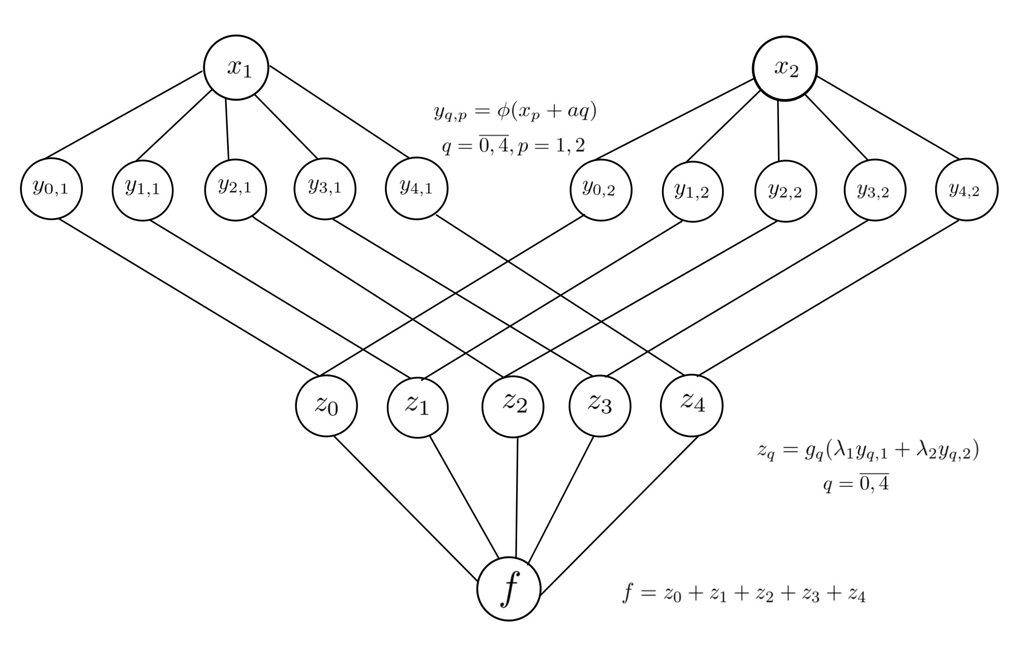
Eq. (1.1) has the following interpretation as a feedforward neural network consisting of an input layer, two hidden layers and an output layer. The input layer having $d$ neurons sends signals $x_{1},...x_{d}$ to the first hidden layer with $d(2d+1)$ neurons and the activation function $\varphi$. The $(q,p)$-th neuron $y_{q,p}$ ($0\leq q\leq 2d,$ $1\leq p\leq d$) produces the signal $\varphi(x_{p}+aq)$. These signals are sent to the second hidden layer consisting of $2d+1$ neurons and the activation functions $g_{q}$. The $q$-th neuron $z_{q}$ ($0\leq q\leq 2d$) produces the signal $g_{q}\left(\sum_{p=1}^{d}\lambda_{p}y_{q,p}\right)$. Finally, the output layer with the unique output neuron just sums up these last signals to produce the number $f(x_{1},...x_{d})$. Feedforward neural networks with this structure are usually called the Kolmogorov neural networks. Figure 1 displays Kolmogorov’s neural network in case of $d=2$.

Figure 1: The neural network interpretation of Kolmogorov’s superposition theorem.

The relevance of Kolmogorov’s superposition theorem to neural networks was first observed by Hecht-Nielsen [8]. In Hecht-Nielsen’s interpretation the Kolmogorov neural network (called in [8] Kolmogorov’s mapping neural network) had three layers, two hidden layers in Fig. 1 were identified as a single layer. Although Kolmogorov’s theorem reveals the profound character of feedforward neural networks to precisely represent each continuous function, it was considered by some authors as non-constructive. For example, Girosi and Poggio pointed out that Kolmogorov’s network is not useful. In [6] they argued that for an implementation of a network that has good properties, the functions corresponding to the layers in the network have to be smooth, which is not the case for the functions $\varphi$ and $g_{q}$ in Kolmogorov’s network. This criticism was addressed by Kůrkova [21, 22] pointing out that the relevance of Kolmogorov’s superposition theorem to approximation by neural networks is different. Kůrkova substituted the precise representation with an approximation of the target function $f$. For this purpose she used sigmoidal functions $\sigma$ (which is defined as a function with the property $\lim_{t\rightarrow-\infty}\sigma(t)=0$ and $\lim_{t\rightarrow+\infty}\sigma(t)=1$) and finite linear combinations $\sum_{k}c_{k}\sigma(w_{k}x-\theta_{k})$ to approximate functions of one variable, in particular Kolmogorov’s inner universal and outer functions. As a result, the number of terms in the outer sum was increased, but her method enabled an estimation of the number of hidden neurons depending on the approximation accuracy $\varepsilon$. Note that in [22] the number of hidden neurons increases when the approximation accuracy $\varepsilon\rightarrow\infty$.

The above dependency of $\varepsilon$ on the number of neurons was eliminated in Nakamura, Mines, and Kreinovich [25]. They developed algorithms that generate the activation functions with guaranteed accuracy and keep number of hidden neurons independent of $\varepsilon$. All operations and functions in [25] were defined constructively, which means that they are implementable in a computer program. However, as noted by the authors of [25], the algorithms that they constructed in the proofs are very complicated and not suitable for practical usage. For other approximative, but constructive approaches to function approximation by using Kolmogorov’s superposition theorem, see [5, 9, 26].

Using Kůrkova’s ideas, Sprecher and Katsura [16] constructed a sequence of functions $\left\{\varphi_{n}\right\}_{n=1}^{\infty}$ that converges to the inner function $\varphi$ and constructed $2d+1$ series of functions that converge to the outer functions $g_{q}$ in (1.1).

Later Sprecher [31, 32] developed a numerical algorithm for the computation of the inner and outer functions in (1.1). In these papers, the inner function $\varphi$ is defined as an extension of a function which is explicitely defined on the set of so-called terminating rational numbers. Note that these numbers are dense in $\mathbb{R}$. He proved continuity and monotonicity of the resulting function $\varphi$.

The papers [31, 32] were discussed in Köppen [20], where it was pointed out that Sprecher’s function $\varphi$ does not possess the continuity and monotonicity properties. To fill this gap, Köppen suggested a modified inner function and stated its continuity. He defined $\varphi$ recursively on the same set of terminating rational numbers $\mathcal{D}$ and claimed that this recursion terminates. Köppen assumed that there exists an extension from $\mathcal{D}$ to $\mathbb{R}$ as in Sprecher’s construction and that this extended $\varphi$ is monotone increasing and continuous, but he did not give a proof for it. Such a proof was given in Braun and Griebel [2] and Braun [3]. That is, it was shown that Köppen’s $\varphi$ indeed exists, i.e., it is well defined and has the necessary continuity and monotonicity properties.

In this section we show that the above Theorem 1.1 can be generalized to discontinuous bounded and also to all unbounded functions. In addition, we prove that in all cases the outer functions $g_{q}$ can be replaced by a single outer function $g$.

Obviously, all functions on a given compact set $X$ can be divided into the following three nonintersecting classes. These are the classes of continuous, discontinuous bounded and unbounded functions. Note that if a function is continuous on $X$, then it is automatically bounded. The following theorem gives a precise representation formula for each of these classes.

Theorem 2.1. Assume$~{}d\geq 2$ and $\gamma\geq 2d+2$ are given integers and $\mathbb{I}=[0,1]$. Set $a=\left[\gamma(\gamma-1)\right]^{-1},$ $\lambda_{1}=1,\lambda_{p}=\sum_{r=1}^{\infty}\gamma^{-(p-1)(d^{r}-1)/(d-1)}$ for $p=2,3,...,d$ and $b_{q}=(2d+1)q$ for $q=0,1,...,2d$. Then there exists a universal monotonic increasing function $\varphi$ of the class $Lip[\ln 2/\ln\gamma]$ with the property:

Each $d$-variable function $f:\mathbb{I}^{d}\rightarrow\mathbb{R}$ can be precisely represented in the form

$$f(x_{1},...x_{d})=\sum_{q=0}^{2d}g\left(\sum_{p=1}^{d}\lambda_{p}\varphi(x_{p}+aq)+b_{q}\right),$$

where $g$ is a one-variable function depending on $f$. If $f$ is continuous, then $g$ can be chosen continuous as well. If $f$ is discontinuous bounded, then $g$ is discontinuous bounded; and if $f$ is unbounded, then $g$ is unbounded.

Theorem 2.1 gives rise to the following feedforward neural network model. This model contains four layers: the input layer with $d$ neurons $x_{1},...x_{d}$, the first hidden layer with $d(2d+1)$ neurons $y_{q,p}$, $0\leq q\leq 2d,$ $1\leq p\leq d$, the second hidden layer with $2d+1$ neurons $z_{q}$, $0\leq q\leq 2d$, and the output layer with a single neuron $w$. Activation functions of the first and second hidden layers are $\varphi$ and $g$, respectively. The connecting rules between the layers are as follows:

The input layer : $$\text{ }x_{1},...x_{d};$$

The first hidden layer : $$\text{ }y_{q,p}=\varphi(x_{p}+aq)\text{ for }q=0,1,...,2d;~{}p=1,...,d;$$

The second hidden layer : $$\text{ }z_{q}=g\left(\sum_{p=1}^{d}\lambda_{p}y_{q,p}+b_{q}\right)\text{ for }q=0,1,...,2d;$$

The output layer : $$\text{ }w=\sum_{q=0}^{2d}z_{q}.$$

Theorem 2.1 means that any multivariate function $f(x_{1},...x_{d})$ can be implemented by such a network. That is, $w=f(x_{1},...x_{d})$. The only parameter depending on $f$ is the activation function $g$ of the second hidden layer. It carries continuity and boundedness properties of the given $f$. More precisely, $g$ is continuous if $f$ is continuous, $g$ is discontinuous bounded if $f$ is discontinuous bounded, and $g$ is unbounded if $f$ is unbounded.

Proof. Using Sprecher’s result, it is easy to prove (2.1) for continuous $f:\mathbb{I}^{d}\rightarrow\mathbb{R}$. Note that for such a function representation (1.1) is valid. In the proof of (1.1) $\varphi$ was constructed in such a way that $\varphi(\mathbb{I})=\mathbb{I}$ and $\varphi(x+1)=\varphi(x)+1$ for $x\in\mathbb{I}$ (see [31]). This means that $\varphi([0,2])=[0,2].$ Since $0\leq x_{p}+aq<2$ for all indices $p$ and $q$, we have $0\leq\varphi(x_{p}+aq)<2.$ On the other hand it is not difficult to check that $\max\left\{\lambda_{1},...,\lambda_{p}\right\}=1.$ Hence the ranges of all the functions $\sum_{p=1}^{d}\lambda_{p}\varphi(x_{p}+aq)$ in (2.1) fall into $[0,2d]$. It follows that the ranges of the functions

$$\Psi_{q}(x_{1},...x_{d}):=\sum_{p=1}^{d}\lambda_{p}\varphi(x_{p}+aq)+b_{q},~{}~{}q=0,1,...,2d,$$

are pairwise disjoint.

Let $Y_{q}$ denote the range of $\Psi_{q}(x_{1},...x_{d})$. That is,

$$Y_{q}:=\Psi_{q}(\mathbb{I}^{d})\text{ for all }q=0,1,...,2d.$$

Set

$$Y:=\cup_{q=0}^{2d}Y_{q}.$$

Note that all $Y_{q}$ and $Y$ are compact sets. Construct the function $g$ on $Y$ by the following way:

$$g(y):=g_{q}(y-b_{q})\text{ if }y\in Y_{q},\text{ }q=0,1,...,2d.$$

Since $Y_{i}\cap Y_{j}\neq\emptyset$, for all $0\leq i,j\leq 2d$, $i\neq j$, this formula makes $g$ a well-defined function on $Y.$ Clearly, $g$ is continuous on $Y$ and we can extend $g$ by continuity to the whole $\mathbb{R}$. In fact, there are many ways of doing this. Now taking (2.2) into account in (1.1), we obtain (2.1).

Now let us prove (2.1) for bounded $f:\mathbb{I}^{d}\rightarrow\mathbb{R}$. We use the above proved fact that representation (2.1) holds for continuous multivariate functions defined on $\mathbb{I}^{d}$. Let for any compact set $X$, $C(X)$ and $B(X)$ stand for the spaces of continuous functions on $X$ and bounded functions on $X$, respectively.

Consider the operator

$$T:C(Y)\rightarrow C(\mathbb{I}^{d}),\text{ }Tg=\sum_{q=0}^{2d}g\left(\sum_{p=1}^{d}\lambda_{p}\varphi(x_{p}+aq)+b_{q}\right).$$

Since (2.1) is valid for all $f\in C(\mathbb{I}^{d})$, the operator $T$ in (2.3) is a surjection. Consider also the dual spaces $C(Y)^{\ast}$ and $C(\mathbb{I}^{d})^{\ast}.$ These are the spaces of regular real-valued measures of finite total variation defined on Borel subsets of $Y$ and $\mathbb{I}^{d}$, respectively.

The conjugate operator $T^{\ast}:C(\mathbb{I}^{d})^{\ast}\rightarrow C(Y)^{\ast}$ has the form

$$T^{\ast}\mu=\sum_{q=0}^{2d}\Psi_{q}\circ\mu.$$

Here $\Psi_{q}\circ\mu$ is a measure in $C(Y_{q})^{\ast}$, which is defined as follows

$$\left[\Psi_{q}\circ\mu\right](Q)=\mu(\Psi_{q}^{-1}(Q)),\text{ for all }Q\in\mathcal{B}_{q}\text{,}$$

where $\mathcal{B}_{q}$ is the set of Borel subsets of $Y_{q}.$

It is a well known fact in Functional Analysis that an operator $F:U\rightarrow V$ between Banach spaces $U$ and $V$ is a surjection if and only if the conjugate operator $F^{\ast}:V^{\ast}\rightarrow U^{\ast}$ is one-to-one and closed (and vice versa). The last is equivalent to the inequality

$$\left\|x\right\|\leq\epsilon\left\|F^{\ast}x\right\|\text{,}$$

for all $x\in V^{\ast}$ and some $\epsilon>0$ (see, e.g., [27, Ch. 4]). Applying this fact to our problem, we obtain that there exists a positive number $\epsilon$ such that the inequality

$$\left\|\mu\right\|\leq\epsilon\left\|T^{\ast}\mu\right\|=\epsilon\left\|\sum_{q=0}^{2d}\Psi_{q}\circ\mu\right\|\leq\epsilon\sum_{q=0}^{2d}\left\|\Psi_{q}\circ\mu\right\|$$

holds for all $\mu\in C(\mathbb{I}^{d})^{\ast}$.

For any compact set $X$, consider a linear space $l_{1}(X)$ consisting of discrete measures in $X$. That is, $\nu\in l_{1}(X)$ means that

$$\nu=\sum_{i=1}^{\infty}a_{i}\delta_{t_{i}},\text{ }\left\|\nu\right\|=\sum_{i=1}^{\infty}\left|a_{i}\right|<\infty$$

where $\{a_{i}\}_{i=1}^{\infty}$ is a sequence of real numbers such that $\sum_{i=1}^{\infty}\left|a_{i}\right|<\infty,$ $\{t_{i}\}_{i=1}^{\infty}$ is a sequence in $\mathbb{I}^{d}$ and $\delta_{t_{i}}$ are points masses at $t_{i}.$

Note that $l_{1}(X)\subset C(X)^{\ast}$. Thus (2.4) holds also for all $\mu\in l_{1}(\mathbb{I}^{d}).$

Now construct the following Banach space

$$S=\left\{\nu=(\nu_{0},...,\nu_{2d}):\nu_{q}\in l_{1}(Y_{q}),~{}0\leq q\leq 2d\right\},\text{ }\left\|\nu\right\|=\sum_{q=0}^{2d}\left\|\nu_{q}\right\|.$$

Consider its dual $S^{\ast}$. Since for any $X$, the dual of $l_{1}(X)$ is the space of bounded functions on $X$ (see, e.g., [4, Ch. 4]), the space $S^{\ast}$ has the following structure:

$$S^{\ast}=\left\{g=(g_{0},...,g_{2d}):g_{q}\in B(Y_{q}),~{}0\leq q\leq 2d\right\},\text{ }\left\|g\right\|=\max_{0\leq q\leq 2d}\left\|g_{q}\right\|.$$

Note that $g\in S^{\ast}$ acts on $\nu\in S$ as follows

$$g[\nu]=\sum_{q=0}^{2d}\int_{Y_{q}}g_{q}d\nu_{q}.$$

Consider the operator

$$Z:l_{1}(\mathbb{I}^{d})\rightarrow S;~{}Z(\mu)=\left(\Psi_{0}\circ\mu,...,\Psi_{2d}\circ\mu\right)$$

and its conjugate

$$Z^{\ast}:S^{\ast}\rightarrow l_{1}(\mathbb{I}^{d})^{\ast}.$$

Note that by the definition of conjugate operator

$$Z^{\ast}g[\mu]=g[Z\mu]=\sum_{q=0}^{2d}\int_{Y_{q}}g_{q}d(\Psi_{q}\circ\mu)=\sum_{q=0}^{2d}\int_{\mathbb{I}^{d}}g_{q}\circ\Psi_{q}d\mu=\int_{\mathbb{I}^{d}}\left(\sum_{q=0}^{2d}g_{q}\circ\Psi_{q}\right)d\mu.$$

Therefore,

$$Z^{\ast}g=\sum_{q=0}^{2d}g_{q}\circ\Psi_{q}.$$

Again by the above mentioned fact of Functional Analysis the operator $Z^{\ast}$ is surjective if and only if there exists $\epsilon>0$ such that

$$\left\|\mu\right\|\leq\epsilon\left\|Z\mu\right\|=\epsilon\sum_{q=0}^{2d}\left\|\Psi_{q}\circ\mu\right\|$$

holds for all $\mu\in l_{1}(\mathbb{I}^{d})$. But we have seen above in (2.4) that this inequality indeed holds for all $\mu\in C(\mathbb{I}^{d})^{\ast}$, hence for all $\mu\in l_{1}(\mathbb{I}^{d})\subset C(\mathbb{I}^{d})^{\ast}$. We obtain that $Z^{\ast}$ is a surjective operator and hence its range is all of $l_{1}(\mathbb{I}^{d})^{\ast}=B(\mathbb{I}^{d}).$ Comparing this assertion with (2.5) gives that for any bounded function $f\in B(\mathbb{I}^{d})$ the representation

$$f=\sum_{q=0}^{2d}g_{q}\circ\Psi_{q},$$

is valid for some bounded $g_{q}\in B(Y_{q}).$ Since the sets $Y_{q},$ $q=0,1,...,2d,$ are pairwise disjoint, we can construct a single function $g$ as in (2.2), which is well defined and bounded on $Y$. One can extend $g$ to the whole real line in such a way that $g$ remains bounded also on $\mathbb{R}$. Thus for any $f\in B(\mathbb{I}^{d})$ we have the precise representation

$$f(x_{1},...,x_{d})=\sum_{q=0}^{2d}g(\Psi_{q}(x_{1},...,x_{d})),$$

where $g\in B(\mathbb{R})$. If $f$ is bounded and discontinuous, then $g$ will be discontinuous as well, otherwise the right-hand side of (2.6) will be a continuous function whereas the left-hand side is discontinuous. This proves the second part of the theorem. It should be remarked that the method of using $l_{1}(X)$ measures in representation of bounded functions on $X$ was introduced by Sternfeld [33] and refined by Khavinson [17, Ch. 1].

Now let us prove the theorem for an unbounded function $f:\mathbb{I}^{d}\rightarrow\mathbb{R}$. In fact, we will prove the validity of (2.1) for any $d$-variable function $f$ defined on $\mathbb{I}^{d}$. Certainly, if $f$ is unbounded, then $g$ must be unbounded too, otherwise the right hand side of (2.1) would be bounded, contradicting the equality in (2.1). In [14], the second author proved a slightly different version of this part, where not a single but $2d+1$ outer functions $g_{q}$ in the representation formula are needed. For completeness we repeat the main details of that proof here and show where and how all that $g_{q}$ can be replaced by a single function $g$.

Again we use the representation formula (2.1) for continuous functions, which has been proved above. In fact, we will use the following concise form of (2.1)

$$f(x_{1},...,x_{d})=\sum_{q=0}^{2d}g(\Psi_{q}(x_{1},...,x_{d})),$$

where $f\in C(\mathbb{I}^{d})$, $g\in C(\mathbb{R})$ and $\Psi_{q}$ are defined above. From (2.7) we can obtain the following important property of the family of functions $\left\{\Psi_{q}\right\}_{q=0}^{2d}$, which we formulate as a lemma.

Lemma 2.1. For any finite set $\{\mathbf{x}_{1},...,\mathbf{x}_{n}\}\subset$ $\mathbb{I}^{d}$ the system of equations

$$\sum_{j=1}^{n}\mu_{j}\delta_{\Psi_{q}(\mathbf{x}_{j})}=0,~{}q=0,...,2d,$$

with respect to $\mu_{j}$ has only a zero solution.

In this lemma and in the sequel $\delta_{\mathcal{A}}$ stands for the indicator function of a set $\mathcal{A}\subset\mathbb{R}$. That is,

$$\delta_{\mathcal{A}}(t)=\left\{\begin{array}[]{c}1,\text{ if }t\in\mathcal{A}\\ 0,\text{ if }t\notin\mathcal{A}\end{array}\right..$$

Note that in (2.8) $\delta_{\Psi_{q}(\mathbf{x}_{j})}$ are indicator functions of the single point sets $\{\Psi_{q}(\mathbf{x}_{j})\}$.

Let us explain Eq. (2.8) in detail. We will see that it stands for a system of certain linear equations. To show this, fix the subscript $q.$ Let the set $\{\Psi_{q}(\mathbf{x}_{j}),$ $j=1,...,n\}$ have $s_{q}$ different values, which we denote by $\gamma_{1}^{q},\gamma_{2}^{q},...,\gamma_{s_{q}}^{q}.$ Then (2.8) implies that

$$\sum_{j}\mu_{j}=0,$$

where the sum is taken over all $j$ such that $\Psi_{q}(\mathbf{x}_{j})=\gamma_{k}^{q}$, $k=1,...,s_{q}$. Thus for fixed $q$ we have $s_{q}$ linear homogeneous equations in $\mu_{1},...,\mu_{n}$. The coefficients of these equations are $0$ and $1$. By varying $q$, we will have $\sum_{q=0}^{2d}s_{q}$ such equations. Thus (2.8), in its expanded form, stands for the system of these equations.

Note that not only $\left\{\Psi_{q}\right\}_{q=0}^{2d}$, but a family of arbitrarily given multivariate functions $\left\{h_{1},...,h_{k}\right\}$ on any set $X$ can generate (2.8). It should be remarked that in this case finite sets $\{\mathbf{x}_{1},...,\mathbf{x}_{n}\}$ satisfying the system of equations (2.8) when there is a nonzero solution $(\mu_{1},...,\mu_{n})$ were exploited under the name of “closed paths” in several works of the second author (see, e.g., [10, 12, 13]).

Let us now prove the lemma. Assume the contrary. Assume that there is a finite set $p=\{\mathbf{x}_{1},...,\mathbf{x}_{n}\}$ in $\mathbb{I}^{d}$ such that the system of equations (2.8) has a nonzero solution $\mu=(\mu_{1},...,\mu_{n})$. Without loss of generality we may assume that all the numbers $\mu_{j}\neq 0$, $j=1,...,n$. Otherwise we can remove all zero components $\mu_{j}$ from $\mu$ and the corresponding $\mathbf{x}_{j}$ (having the same index) from $p$ and consider the resulting sets $\{\mu_{j}\}$ and $\{\mathbf{x}_{j}\}$. Consider the linear functional

$$G_{p}(f)=\sum_{j=1}^{n}\mu_{j}f(\mathbf{x}_{j}),\text{ }G_{p}:C(\mathbb{I}^{d})\rightarrow\mathbb{R}\text{.}$$

This functional annihilates all sums of the form $\sum_{q=0}^{2d}g(\Psi_{q}(x_{1},...,x_{d}))$, and hence, according to (2.7), every function $f\in C(\mathbb{I}^{d})$. That is, $G_{p}(f)=0$ for any $f\in C(\mathbb{I}^{d})$. On the other hand by Urysohn’s lemma (see, e.g., [34, Ch. 5]) there exists a continuous function $f_{0}$ with the property: $f_{0}(\mathbf{x}_{j})=1$ for indices $j$ such that $\mu_{j}>0$; $f_{0}(\mathbf{x}_{j})=-1$ for indices $j$ such that $\mu_{j}<0$; and $-1<f_{0}(\mathbf{x})<1$ for $\mathbf{x}\in\mathbb{I}^{d}\setminus p$. For this function we have $G_{p}(f_{0})=\sum_{j=1}^{n}\left|\mu_{j}\right|\neq 0$. The obtained contradiction means that Eq. (2.8) has only a zero solution $(\mu_{1},...,\mu_{n})$ for any finite subset $\{\mathbf{x}_{1},...,\mathbf{x}_{n}\}\subset\mathbb{I}^{d}$. The lemma has been proved.

Now let us return to the proof of the third part of our theorem. We want to prove that for any function $f:\mathbb{I}^{d}\rightarrow\mathbb{R}$, the following representation holds

$$f(x_{1},...,x_{d})=\sum_{q=0}^{2d}g(\Psi_{q}(x_{1},...,x_{d})),$$

where $g$ is a one-variable function depending on $f$.

Recall that we denoted ranges of $\Psi_{q}$ by $Y_{q}$ and $Y$ is the union of $Y_{q}.$ Consider the following set

$$\mathcal{L}=\{A=\{y_{0},...,y_{2d}\}:\text{if there exists }\mathbf{x}\in\mathbb{I}^{d}\text{ s.t. }\Psi_{q}(\mathbf{x})=y_{q},~{}q=0,...,2d\}$$

Note that $\mathcal{L}$ is not a subset of $Y$. It is a set of some special subsets of $Y.$ Each element of $\mathcal{L}$ is a set $A=\{y_{0},...,y_{2d}\}\subset Y$ with the property that there exists at least one point $\mathbf{x}\in\mathbb{I}^{d}$ such that $\Psi_{q}(\mathbf{x})=y_{q},~{}q=0,...,2d.$ These $\mathbf{x}$ will be called generating points for $A$.

It is almost obvious that in (2.9) for each element $A$ there exists only one generating point $\mathbf{x}\in\mathbb{I}^{d}$. Indeed, if there were two points $\mathbf{x}_{1}$ and $\mathbf{x}_{2}$ for a single $A$ in (2.9), then $\Psi_{q}(\mathbf{x}_{1})=\Psi_{q}(\mathbf{x}_{2})$, $q=0,...,2d$, and hence for the set $\left\{\mathbf{x}_{1},\mathbf{x}_{2}\right\}\subset\mathbb{I}^{d}$ we would have

$$1\cdot\delta_{\Psi_{q}(\mathbf{x}_{1})}+(-1)\cdot\delta_{\Psi_{q}(\mathbf{x}_{2})}\equiv 0,~{}q=0,...,2d.$$

That is, for such $\left\{\mathbf{x}_{1},\mathbf{x}_{2}\right\}$ the system of equations (2.8) would have a nonzero solution $(1;-1).$ But this contradicts Lemma 2.1.

Since in (2.8) each $A\in\mathcal{L}$ corresponds to only one generating point $\mathbf{x}\in\mathbb{I}^{d}$, we can define the following set function

$$\tau:\mathcal{L}\rightarrow\mathbb{R},~{}\tau(A)=f(\mathbf{x}).$$

Consider now a class $\mathcal{S}$ of functions of the form $\sum_{j=1}^{m}r_{j}\delta_{D_{j}},$ where $m$ is a positive integer, $r_{j}$ are real numbers and $D_{j}$ are elements of $\mathcal{L},~{}j=1,...,m.$ We fix neither the numbers $\ m,~{}r_{j},$ nor the sets $D_{j}.$ Clearly, $\mathcal{S\ }$is a linear space. On elements of $\mathcal{S}$, we define the linear functional

$$F:\mathcal{S}\rightarrow\mathbb{R},~{}F\left(\sum_{j=1}^{m}r_{j}\delta_{D_{j}}\right)=\sum_{j=1}^{m}r_{j}\tau(D_{j}).$$

Introduce the linear space:

$$\mathcal{S}^{\prime}=\left\{\sum_{j=1}^{m}r_{j}\delta_{\omega_{j}}\right\},$$

where $m\in\mathbb{N}$, $r_{j}\in\mathbb{R}$, $\omega_{j}\subset Y.$ As above, we do not fix the parameters $m$, $r_{j}$ and $\omega_{j}.$ Note that now we use not only the special subsets $D_{j}$ of $Y$, but all possible subsets $\omega_{j}\subset Y$. Obviously, the space $\mathcal{S}^{\prime}$ is larger than $\mathcal{S}$. Consider the linear extension of $F$ to the space $\mathcal{S}^{\prime}$, which we denote by $F^{\prime}$. That is, $F^{\prime}:\mathcal{S}^{\prime}\rightarrow\mathbb{R}$ and $F^{\prime}(z)=F(z)$ for all $z\in\mathcal{S}$.

Define the following functions:

$$g_{q}:Y_{q}\rightarrow\mathbb{R},\text{ }g_{q}(y_{q}):=F^{\prime}(\delta_{y_{q}}),\text{ }q=0,...,2d.$$

Since the sets $Y_{q}$ are pairwise disjoint we can also define the single function

$$g:Y\rightarrow\mathbb{R}\text{, }g(y)=g_{q}(y),\text{ if }y\in Y_{q}\text{.}$$

Clearly, (2.10) correctly defines $g$ on the whole $Y$, the union of ranges of $\Psi_{q}$.

Let now $\mathbf{x}=(x_{1},...,x_{d})$ be an arbitrary point in $\mathbb{I}^{d}.$ Obviously, $\mathbf{x}$ is a generating point for some set $A=\{y_{0},...,y_{2d}\}\in\mathcal{L}$. Thus we can write that

$$f(\mathbf{x})=\tau(A)=F(\delta_{A})=F\left(\sum_{q=0}^{2d}\delta_{y_{q}}\right)=F^{\prime}\left(\sum_{q=0}^{2d}\delta_{y_{q}}\right)=$$

$$\sum_{q=0}^{2d}F^{\prime}(\delta_{y_{q}})=\sum_{q=0}^{2d}g_{q}(y_{q})=\sum_{q=0}^{2d}g(y_{q})=\sum_{q=0}^{2d}g(\Psi_{q}(\mathbf{x})).$$

This proves the theorem for all functions $f:\mathbb{I}^{d}\rightarrow\mathbb{R}$, hence for unbounded $f$.

3. Conclusions and remarks

The topic on the role of Kolmogorov superposition theorem in neural network theory is still active today (see, e.g., [15, 24, 28, 29]). The research in this area was developed mainly in two directions. In the first direction, the analysis was concentrated on approximative versions of Kolmogorov’s superposition theorem and obtaining corresponding results on neural network approximation (see, e.g., [7, 11, 13, 21, 22, 23]). In the second direction, representation power of Kolmogorov superposition-based neural networks were studied (see, e.g., [1, 14, 16, 30, 31, 32]). Due to these second type works, there is a perspective for a practical usage of the precise representation of multivariate functions by Kolmogorov type neural networks.

This paper studies the Kolmogorov two hidden layer neural network model with one-variable activation functions $\varphi$ and $g$ in the first and second hidden layers, respectively. It shows that each multivariate function $f$ can be precisely represented by this model. All parameters of the network except the second activation $g$ are fixed and do not depend on $f$. The main result proves that if $f$ is continuous, then $g$ can be chosen continuous as well. Further if $f$ is discontinuous bounded, then $g$ is discontinuous bounded; and if $f$ is unbounded, then $g$ is unbounded.

It should be remarked that existence results and construction methods for the universal inner function $\varphi$ were given in the papers [31, 20, 2, 3] (see Introduction). Using these methods one can easily construct the functions $\Psi_{q}$, since all the numbers in their definitions are explicitly known. A numerical algorithm for the parallel computations $g_{q}$ in the representation formula (1.1) was developed in [32]. Taking into account (2.2) one can apply Sprecher’s method for computation of the single outer function $g$. These tips refer to computational aspects of the case when in Theorem 2.1 only continuous functions are involved. A practical construction of $g$ in cases with discontinuous bounded and unbounded functions is not yet known. For such cases Theorem 2.1 gives only a theoretical understanding of the representation problem. This is because for the representation of discontinuous bounded functions we have derived (2.1) from the fact that the range of the operator $Z^{\ast}$ is the whole space of bounded functions $B(\mathbb{I}^{d})$. This fact directly gives us a formula (2.1) but does not tell how the bounded one-variable function $g$ is attained. For the representation of unbounded functions we have used a linear extension of the functional $F$, existence of which is based on Zorn’s lemma (see, e.g., [19, Ch. 3]). Application of Zorn’s lemma provides no mechanism for practical construction of such an extension. Zorn’s lemma helps to assert only its existence.

References

- [1] V. Brattka, From Hilbert’s 13th problem to the theory of neural networks: Constructive aspects of Kolmogorov’s superposition theorem, In: Kolmogorov’s Heritage in Mathematics, Springer, Berlin, 2007, 253–280.
- [2] J. Braun and M. Griebel, On a constructive proof of Kolmogorov’s superposition theorem, Constr. Approx. 30 (2009), no. 3, 653–675.
- [3] J. Braun, An application of Kolmogorov’s superposition theorem to function reconstruction in higher dimensions, Ph.D. dissertation, Universitat Bonn, 2009.
- [4] N. Dunford and J. T. Schwartz, Linear operators. Part I, Interscience, New York, 1959.
- [5] R. J. P. de Figueiredo, Implications and applications of Kolmogorov’s superposition theorem, IEEE Trans. Automatic Control, AC-25 (1980), 1227–1231.
- [6] F. Girosi and T. Poggio, Representation properties of networks: Kolmogorov’s theorem is irrelevant, Neural Comp., 1 (1989), 465–469.
- [7] N. J. Guliyev and V. E. Ismailov, Approximation capability of two hidden layer feedforward neural networks with fixed weights, Neurocomputing 316 (2018), 262–269.
- [8] R. Hecht-Nielsen, Kolmogorov’s mapping neural network existence theorem, In: Proc. I987 IEEE Int. Conf. on Neural Networks, IEEE Press, New York, 1987, vol. 3, 11–14.
- [9] B. Igelnik and N. Parikh, Kolmogorov’s spline network, IEEE Trans. Neural Netw., 14 (2003), 725–733.
- [10] V. E. Ismailov, A note on the representation of continuous functions by linear superpositions, Expo. Math. 30 (2012), 96–101.
- [11] V. E. Ismailov, On the approximation by neural networks with bounded number of neurons in hidden layers, J. Math. Anal. Appl. 417 (2014), no. 2, 963–969.
- [12] V. E. Ismailov, On the uniqueness of representation by linear superpositions, Ukrainian Math. J. 68 (2017), no. 12, 1874–1883.
- [13] V. E. Ismailov, Ridge functions and applications in neural networks, Mathematical Surveys and Monographs, 263. American Mathematical Society, 2021, 186 pp.
- [14] V. E. Ismailov, A three layer neural network can represent any multivariate function. J. Math. Anal. Appl. 523 (2023), no. 1, Paper No. 127096, 8 pp.
- [15] P. E. T. Jorgensen and J. F. Tian, Superposition, reduction of multivariable problems, and approximation, Anal. Appl. (Singap.) 18 (2020), no. 5, 771–801.
- [16] H. Katsura and D. A. Sprecher, Computational aspects of Kolmogorov’s superposition theorem, Neural Netw., 7 (1994), 455–461.
- [17] S. Ya. Khavinson, Best approximation by linear superpositions (approximate nomography), Translated from the Russian manuscript by D. Khavinson. Translations of Mathematical Monographs, 159. American Mathematical Society, Providence, RI, 1997, 175 pp.
- [18] A. N. Kolmogorov, On the representation of continuous functions of many variables by superposition of continuous functions of one variable and addition. (Russian), Dokl. Akad. Nauk SSSR 114 (1957), 953–956.
- [19] A. N. Kolmogorov, S. V. Fomin, Elements of the theory of functions and functional analysis, Sixth edition. “Nauka”, Moscow, 1989, 624 pp.
- [20] M. Köppen, On the training of a Kolmogorov network, ICANN 2002, Lecture Notes In Computer Science, 2415 (2002), 474–479.
- [21] V. Kůrkova, Kolmogorov’s theorem is relevant, Neural Comp., 3 (1991), 617–622.
- [22] V. Kůrkova, Kolmogorov’s theorem and multilayer neural networks, Neural Netw., 5 (1992), 501–506.
- [23] V. Maiorov and A. Pinkus, Lower bounds for approximation by MLP neural networks, Neurocomputing 25 (1999), 81–91.
- [24] H. Montanelli and H. Yang, Error bounds for deep ReLU networks using the Kolmogorov-Arnold superposition theorem, Neural Netw. 129 (2020), 1–6.
- [25] M. Nakamura, R. Mines, and V. Kreinovich, Guaranteed intervals for Kolmogorov’s theorem (and their possible relation to neural networks), Interval Comput., 3 (1993), 183–199.
- [26] M. Nees, Approximative versions of Kolmogorov’s superposition theorem, proved constructively, J. Comput. Appl. Math., 54 (1994), 239–250.
- [27] W. Rudin, Functional analysis, Second edition. International Series in Pure and Applied Mathematics. McGraw-Hill, Inc., New York, 1991, 424 pp.
- [28] J. Schmidt-Hieber, The Kolmogorov-Arnold representation theorem revisited, Neural Netw. 137 (2021), 119–126.
- [29] Z. Shen, H. Yang, and S. Zhang, Neural network approximation: Three hidden layers are enough, Neural Netw. 141 (2021), 160-173.
- [30] D. A. Sprecher, A universal mapping for Kolmogorov’s superposition theorem, Neural Netw. 6 (1993), 1089–1094.
- [31] D. A. Sprecher, A numerical implementation of Kolmogorov’s superpositions, Neural Netw. 9 (1996), 765–772.
- [32] D. A. Sprecher, A numerical implementation of Kolmogorov’s superpositions II, Neural Netw. 10 (1997), 447–457.
- [33] Y. Sternfeld, Uniformly separating families of functions, Israel J. Math. 29 (1978), 61–91.
- [34] S. Willard, General topology, Addison-Wesley Publishing Co., Reading, Mass.-London-Don Mills, Ont., 1970, 369 pp.