Temperature Dependence of Energy Transport in the $\mathbb{Z}_{3}$ Chiral Clock Model

Abstract

We employ matrix product state simulations to study energy transport within the non-integrable regime of the one-dimensional $\mathbb{Z}_{3}$ chiral clock model. To induce a non-equilibrium steady state throughout the system, we consider open system dynamics with boundary driving featuring jump operators with adjustable temperature and footprint in the system. Given a steady state, we diagnose the effective local temperature by minimizing the trace distance between the true local state and the local state of a uniform thermal ensemble. Via a scaling analysis, we extract the transport coefficients of the model at relatively high temperatures above both its gapless and gapped low-temperature phases. In the medium-to-high temperature regime we consider, diffusive transport is observed regardless of the low-temperature physics. We calculate the temperature dependence of the energy diffusion constant as a function of model parameters, including in the regime where the model is quantum critical at the low temperature. Notably, even within the gapless regime, an analysis based on power series expansion implies that intermediate-temperature transport can be accessed within a relatively confined setup. Although we are not yet able to reach temperatures where quantum critical scaling would be observed, our approach is able to access the transport properties of the model over a broad range of temperatures and parameters. We conclude by discussing the limitations of our method and potential extensions that could expand its scope, for example, to even lower temperatures.

I Introduction

The study of non-equilibrium quantum systems poses a central challenge across various fields of many-body physics, encompassing classical solid-state systems to the recently emphasized dynamics of quantum information [1, 2, 3, 4, 5, 6, 7, 8]. Among numerous pertinent physical occurrences, delving into transport phenomena can unveil intrinsic characteristics of quantum matter and provide a window into the fundamental dynamical processes at play. While the investigation of energy transport has been a longstanding endeavor, the underlying microscopic source of this typical diffusive transport remains somewhat enigmatic even in the present day. Even in the case of locally interacting one-dimensional systems, determining transport characteristics remains a challenging task [9, 10].

Regarding equilibrium in one-dimensional systems, tensor network approaches, especially matrix product state techniques, have demonstrated significant efficacy in characterizing extensive equilibrium systems [11, 12, 13, 14]. However, when entanglement accumulates in a linear fashion over time, the bond dimension experiences exponential growth, consequently amplifying the computational workload. While new approaches have been developed to surpass this entanglement obstacle by devising altered dynamical principles that diverge from the microscopic unitary evolution [15, 16, 3, 17, 18], open quantum system methodologies, which employ an explicit external driving force to guide a system towards its non-equilibrium steady state (NESS), have emerged as a promising avenue for investigating transport properties [19, 20, 21, 22, 23, 24, 25, 26]. In general, directly connecting a system to a reservoir is anticipated to diminish the entanglement within the system, making it plausible to investigate transport phenomena through a low-entanglement simulation by utilizing an open quantum system methodology.

Nevertheless, how to efficiently implement reservoirs that induce a NESS is still a crucial question. It is essential to employ an open quantum system framework with well-optimized reservoir configurations to induce a NESS, and this can be categorized into different approaches. A first approach could involve establishing a reservoir configuration of infinite size and then eliminating the reservoir’s degrees of freedom through a tracing-out process. Nevertheless, it becomes evident that the resultant master equation exhibits temporal non-locality, and its memory kernel proves overly intricate for practical solvability [27]. For instance, the Redfield master equation [28], which is derived through additional approximations, remains challenging to practically solve.

A more practical strategy involves searching for an evolution equation for the density matrix of the system that can effectively characterize the NESS condition. In this particular situation, the Lindblad master equation [29, 30], which can be obtained via further approximations, possesses two crucial attributes: complete positivity with trace preservation and dynamic semigroup behavior. As a result, it provides a computationally feasible framework. In the case of a system exhibiting good thermalization properties, opting for appropriate local Lindblad operators (which represent the influence of reservoirs) exclusively at the chain’s edges leads to a coherent bulk dynamics primarily governed by the system’s Hamiltonian. These applications can be extended to low-temperature transport scenarios, where intricate phase diagrams need to be taken into account. It has been argued that many systems, including non-interacting and interacting fermions as well as strongly interacting spins, can achieve thermalization under the condition of infinitely large and weakly damped reservoirs [24, 31]. However, achieving reliable thermalization at low temperatures is commonly constrained by various obstacles, such as the system’s intrinsic energy scales and the slow dynamics for attaining a steady state. So designing jump operators that can effectively drive the system to equilibrium remains a challenging task, one that calls for exploration and experimentation.

Here we study energy transport in a $\mathbb{Z}_{3}$ chiral clock model [32, 33, 34, 35, 36, 37, 38] with boundary driving, with a focus on pushing the current methods to their limits. The chiral clock model has been extensively explored from a theoretical standpoint, driven in part by its relevance to a novel experimental setup involving trapped cold atoms [39]. Its low-temperature physics involves a symmetry-breaking quantum phase transition [40], and a prominent aspect of the model is its distinctive property dynamical critical exponent, $z\neq 1$, at criticality [41, 42, 43]. While substantial advancements have been made in exploring the phase transition characteristics of the model through both field-theoretical and numerically-based Density Matrix Renormalization Group (DMRG) approaches [44], the dynamical aspects remain inadequately comprehended. Certain prior investigations have delved into energy transport within this model, including a generalized hydrodynamics framework at a critical integrable point [45], a NESS approach involving tailored Lindblad operators with a constant bath temperature [46] and a DMRG approach for the finite temperature thermal conductivity along a line of integrable points [47]. Nevertheless, there remains considerable potential for further exploration. Given the model’s non-integrable nature and gapless behavior at its quantum critical points, one could anticipate effective thermalization within a certain temperature range. Furthermore, its gapless attribute potentially facilitates investigations into novel regimes of low-temperature transport, opening up the potential for exploring exotic quantum critical transport phenomena. Additionally, it’s worth highlighting that the model extends the transverse field Ising model by enlarging the local Hilbert space from dimension $2$ to $3$. This enlargement provides an opportunity to thoroughly assess the computational capabilities of methods aimed at approximating the thermalized state.

In this study, we explore the finite temperature transport properties of the $\mathbb{Z}_{3}$ chiral clock model by imposing a temperature gradient across the system, which can be achieved with manipulation of the parameters of the bath operators. Similar to the scenario observed in typical non-integrable interacting spin-$1/2$ systems, we anticipate that the model exhibits an efficient NESS description that encapsulates a meaningful effective temperature pertaining to energy transport. While the expanded local state space considerably increases computational complexities, it remains feasible to apply the approach to systems over a range of temperatures that large enough to see behavior consistent with the thermodynamic limit. The system’s effective temperature is evaluated using the thermometry method outlined in Ref. [48], which relies on comparing steady-state local density matrices to their thermal equilibrium counterparts, quantified through a measure of trace distance.

As an initial exploration, we examine the energy transport within the model across both its gapless and gapped phases, focusing on relatively high temperatures for the analysis. Consequently, we observe conventional diffusive transport irrespective of the model’s symmetries and gap magnitude. Subsequently, our attention shifts towards the model’s gapless point, where we assess the temperature-dependent behavior of the energy diffusion constant by progressively reducing the bath temperature. The effective temperature exhibits a linear correlation with the bath temperature before eventually reaching a non-zero saturation point, comparable to the model’s characteristic energy scale, $J$. This behavior mirrors our earlier findings obtained through an analysis of smaller system sizes in Ref. [31]. We uncover a resemblance between the temperature dependency of the gapless chiral clock model and the chaotic spin-$1/2$ XZ model [48]. At the lowest effective temperature attained in our simulations, the diffusivity appears to reside within an intermediate-temperature range when compared to the power-series expansion with respect to inverse temperature.

This paper is structured as follows. First, the $\mathbb{Z}_{3}$ chiral clock model is introduced in Sec. II. Then, in Sec. III, we outline the boundary open system configuration and methods to estimate the effective temperature and the transport coefficients in question. In Sec. IV we present the finite temperature transport characteristics of the system. Finally, we provide analyses of our findings and explore potential extensions in Sec. V.

II The $\mathbb{Z}_{3}$ Chiral Clock Model

Figure 1: The energy gap of the $\mathbb{Z}_{3}$ chiral clock model for $\phi=0$. The gap is computed using DMRG on a one-dimensional chain with a length of $L=200$ and a bond dimension of $\chi=200$. The depicted black region represents the gapless regime, indicating instances of direct transitions for small $\theta$ values and the intermediate incommensurate regime for larger $\theta$. The yellow and red circles in the middle of the map are the chosen critical points of the energy transport study. The green stars represent selected points to study slightly gapped models. In particular, temperature-dependent transport of the model is considered at the red point.

In this investigation, we analyze energy transport within a one-dimensional chain of open boundary conditions for the $\mathbb{Z}_{3}$ chiral clock model (CCM). The Hamiltonian of the CCM for a total chain length $L$ is given by [41, 42, 43]

$$H_{\text{CCM}}=-fe^{-i\phi}\sum_{j=1}^{L}\tau^{\dagger}-Je^{-i\theta}\sum_{j=1}^{L-1}\sigma_{j}^{\dagger}\sigma_{j+1}+\mathrm{h.c.},$$ (1)

where $\tau_{i}$ and $\sigma_{i}$ are the local three-state operators at site $i$. It turns out that $\tau$ and $\sigma$ satisfy following relations

$$\tau^{3}=\sigma^{3}=\mathbb{1},\quad\sigma\tau=\omega\tau\sigma;\quad\omega=e^{2\pi i/3}.$$ (2)

In particular, we choose the explicit matrix representations

$$\tau=\begin{pmatrix}1&0&0\\ 0&\omega&0\\ 0&0&\omega^{2}\end{pmatrix},\quad\sigma=\begin{pmatrix}0&1&0\\ 1&0&0\\ 0&0&1\end{pmatrix}$$ (3)

for $\tau$ and $\sigma$ analogous to the Pauli matrices $\sigma_{z}$ and $\sigma_{x}$ for spin-1/2 systems, respectively. Utilizing these formulations, the $\mathbb{Z}_{3}$ chiral clock model can be seen as an extension of the transverse field Ising model, featuring a broader local Hilbert space of dimension $d=3$. The Hamiltonian presented above comprises four parameters: the on-site spin flip strength and the two-site interaction strength, which are governed by the scalar parameters $f$ and $J$, respectively. The remaining pair of parameters, $\phi$ and $\theta$, introduce distinct “chiralities” to the model.

These many parameters contribute to the model’s intricate phase diagram. As implied by its name, the model exhibits a global $\mathbb{Z}_{3}$ symmetry, which is associated with the operator $\mathcal{G}=\prod_{i}\tau_{i}$. Similar to the behavior of the transverse field Ising model, each coupling strength, $f$ and $J$, define distinct regions within the phase diagram. Consequently, when $f\gg J$, one can anticipate a disordered phase, while on the opposite side of the phase diagram with $f\ll J$, a $\mathbb{Z}_{3}$ ordered phase becomes apparent.

The symmetry properties of the model can be further elucidated by the introduction of three operators, charge conjugation $\mathcal{C}$, spatial parity $\mathcal{P}$, and time reversal $\mathcal{T}$. The following symmetry transformation relations are satisfied by these operators [43]:

$$\mathcal{C}\sigma_{i}\mathcal{C}=\sigma_{i}^{\dagger}, \quad\mathcal{C}\tau_{i}\mathcal{C}=\tau_{i}^{\dagger},\quad\mathcal{C}^{2}=\mathbb{1},$$ (4)

$$\mathcal{P}\sigma_{i}\mathcal{P}=\sigma_{-i}, \quad\mathcal{P}\tau_{i}\mathcal{P}=\tau_{-i},\quad\mathcal{P}^{2}=\mathbb{1},$$ (5)

$$\mathcal{T}\sigma_{i}\mathcal{T}=\sigma_{i}^{\dagger}, \quad\mathcal{T}\tau_{i}\mathcal{T}=\tau_{i},\quad\mathcal{T}^{2}=\mathbb{1}.$$ (6)

The model can have other discrete symmetries depending on the values of parameters $\phi$ and $\theta$ due to the above relationships. When the chiralities are absent ($\phi=\theta=0$), the model exhibits the presence of all three of these symmetries, leading to the model’s reduction into the three-state quantum Potts model [49, 50]. However, when both $\theta\neq 0$ and $\phi\neq 0$, the discrete spacetime symmetry is solely a composite of $\mathcal{C}\mathcal{P}\mathcal{T}$, with no individual symmetry remaining intact. In contrast, either the $\phi=0$ or $\theta=0$ scenario retains separate time-reversal and parity symmetries, wherein the charge conjugation operator $\mathcal{C}$ is coupled with either $\mathcal{P}$ or $\mathcal{C}$, respectively. Notably, the spatial chirality $\theta$ introduces incommensurate floating phases in relation to the periodicity of the underlying lattice [51].

In addition, there is a special parameter curve $f\cos(3\phi)=J\cos(3\theta)$ where the CCM becomes integrable [52] and it further exhibits what is known as “superintegrability” at $\phi=\theta=\pi/6$ [53, 54]. Integrability offers a broad range of methods to manipulate the model, but transport properties near the integrable point are still veiled.

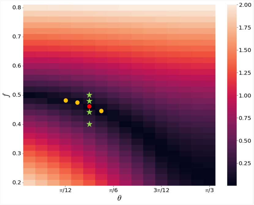
For the sake of simplicity, our study focuses exclusively on models characterized by $\phi=0$ and $f=1-J$. This specific choice has been extensively examined in previous literature [42, 43]. Notably, we specifically opt for several quantum critical points, where direct phase transitions occur as established by Ref. [42]. These particular points are also acknowledged for their gapless nature, and our previous investigations (Ref.  [31]) have highlighted significant constraints when simulating low-temperature transport under these conditions. Furthermore, we extend our analysis to encompass both mildly and fully gapped regimes, achieved by strategically selecting representative points. This approach aims to explore the potential occurrence of crossovers in transport properties. We present the corresponding energy gap map of the model in Figure 1.

III Methods

Figure 2: Illustrative representation of the boundary-driven transport setup. Thermal baths with temperatures $T_{L}$ and $T_{R}$ are produced at both ends of the system using the Lindbladian operator $L_{jk}$. In the depicted scenario, 3-site bath operators are shown, facilitating the establishment of the non-equilibrium steady state. The energy current $j_{E}$ traversing the system is an outcome of this dynamic arrangement.

III.1 Tensor Network Simulation Setup

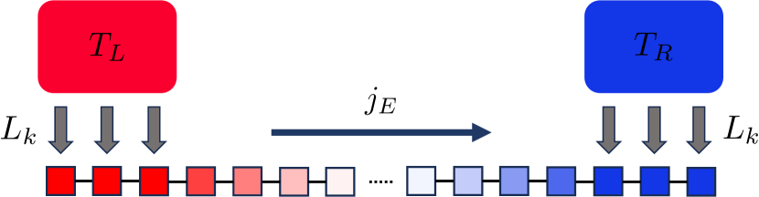
The non-equilibrium configuration depicted in Fig. 2 presents a one-dimensional chain subjected to boundary driving, with two bath assemblies connected at its ends, to investigate energy transport phenomena. To simulate the evolution of a system connected to an environment as described by the bath setup, Markovian dissipative dynamics can be employed in this arrangement. The system’s interaction with the environment is effectively accounted for using a superoperator representation of $\mathcal{L}$. This situation is well-characterized by the GKLS Master equation [29, 30]

$$\frac{d\rho}{dt}=\mathcal{L}(\rho)\equiv-i[H,\rho]+\sum_{jk}\left(L_{jk}\rho L_{jk}^{\dagger}-\frac{1}{2}\{L_{jk}^{\dagger}L_{jk},\rho\}\right),$$ (7)

where $H$ is the Hamiltonian of the system and $L_{jk}$ are Lindblad bath operators, which encode the information of the interaction between the system and the environment, that exclusively operate on the two ends of the one-dimensional chain. The formulation of these operators is guided by the thermal equilibrium states of the system’s Hamiltonian. When the Hamiltonian $H$ is absent, these operators drive the rightmost and leftmost $M$ (bath size) end sites of the system toward its thermal state $\rho_{B}$ at temperature $T_{B}$. A comprehensive description of an arbitrary-size version of $L_{jk}$ is provided in an Appendix of our previous paper [31].

We start by decomposing the Hamiltonian into three components as $H=H_{S}+H_{B}+gH_{I}$. Here, $H_{S}$, $H_{B}$, and $H_{I}$ represent the sub-Hamiltonians that characterize the system (bulk), bath, and their interaction, respectively. In the above decomposition, $g$ serves as a dimensionless coupling governing the degree of interaction between the system and the environment. We set $g=1$ throughout this study to enhance the convergence of the NESS. Further elaboration on this matter can be found in Sec. IV.

When considering the coupling between the bath and Hamiltonian, the steady state of the system deviates from its anticipated thermal equilibrium. As long as it remains feasible to identify an effective temperature for the system, the current setup remains applicable. Within our configuration, the temperature gradient is generated by maintaining different temperatures for the left and right bath operators. Specifically, we assign $T_{L}=1.2T_{B}$ to the left and $T_{R}=0.8T_{B}$ to the right bath operator. This deliberate difference in temperature at the two ends is chosen to provide a clear energy profile and energy current output. Simultaneously, it ensures a moderate variation in the final effective temperature between the two ends, a factor of significance in the determination of the effective bulk temperature.

The equation Eq. (7), known as the master equation, provides a means to describe the time evolution of the density matrix. This implies that the state $\rho(t)$ of the entire open quantum system at a specific time $t$ can be accurately determined using this formalism. By considering the superoperator $\mathcal{L}$, which encodes both coherent and dissipative dynamics, the NESS $\rho_{\text{NESS}}$ corresponds to a unique fixed point solution where $d\rho_{\text{NESS}}/dt=0$ in Eq. (7). It is important to note that while there is generally a unique NESS solution under well-defined conditions, this might not be the case universally [55]. In particular scenarios, there could be a number of slowly decaying quasi-steady states, especially when the impact of the bath operator is limited to the system edges. Mathematically, the NESS is equivalent to the limit of the solution of the master equation as time approaches infinity: $\rho_{\text{NESS}}=\lim_{t\rightarrow\infty}\rho(t)$. While some exceptions exist, such as cases involving non-interacting [56, 57] and strongly-driven systems [58, 59, 60, 61, 62], it remains challenging to directly solve the complete equation for exact NESS solutions in general. When dealing with generic one-dimensional systems, one of the most promising approaches is the utilization of tensor network-based methods.

For open quantum system simulations, the vectorization of the density matrix proves highly advantageous for representing the given problem within an expanded Hilbert space [63, 64, 65]. This approach involves a super-ket state, denoted as $\lvert\rho\rangle$, which directly signifies the associated density matrix as a vector within the operator Hilbert space. Simultaneously, two different physical operators $X$ and $Y$ can operate on $\rho$ via $\lvert X\rho Y\rangle=Y^{T}\otimes X\lvert\rho\rangle$. Within this framework, the Lindbladian operator described in Eq. (7) is transformed into an equivalent Liouvillian super-operator

$$\begin{split}\mathcal{L}&=-i\left(I\otimes H-H^{T}\otimes I\right)\\ &\qquad+\sum_{\nu}\left(L_{\nu}^{\ast}\otimes L_{\nu}-\frac{1}{2}\left(I\otimes L_{\nu}^{\dagger}L_{\nu}+L_{\nu}^{T}L_{\nu}^{*}\otimes I\right)\right).\end{split}$$ (8)

Using Eq. (8) as a starting point, the time evolution of the super-operator can be realized through the application of the Time Evolving Block Decimation (TEBD) algorithm [66, 67], akin to its use in the Matrix Product State (MPS) formalism. To discretize the time evolution operator $e^{\mathcal{L}t}$, we choose the second-order Suzuki-Trotter decomposition [68, 69, 13] with a time step of $\delta t=0.05$. The cumulative error arising from these approximations remains sufficiently negligible for the specific physical parameters employed in our investigation of energy transport. Given the non-integrable nature of the model, the uniqueness of the NESS is preserved regardless of the initial state. Consequently, we opt for the infinite temperature state as the initial condition in the majority of our simulations. The calculation of the NESS typically demands a considerable amount of time, depending on various simulation parameters. However, within the relevant regimes of our model, a finite simulation time of approximately $t\sim 2000$ generally yields robust convergence. Additional details regarding the simulations are available in Appendix A.

III.2 Local Temperature

Utilizing the tensor network simulation elucidated in the preceding section, we ascertain the non-equilibrium steady state (NESS) of the system. Given our focus on transport properties at finite temperatures, it becomes imperative to deduce the effective temperature associated with the resulting NESS. As we mentioned, owing to the intricate interplay between the system and its bath, the effective temperature can diverge from the bath temperature $T_{B}$. One straightforward method to measure the effective temperature involves comparing the final NESS with the Gibbs state at a given temperature, which entails quantifying the dissimilarity between the two states. This approach becomes viable upon the introduction of the notion of local temperature [70, 71, 72, 73, 74].

This approach allows for an estimation of the effective temperature of the system, under the assumption that the system is in local thermal equilibrium within the NESS [48]. The methodology concentrates on the reduced density matrix of the NESS, which dwells on the accessible size of subsystem $A$. Denoting this reduced density matrix as $\rho_{\text{NESS}}^{A}$, we introduce a thermal state $\rho^{A}(T)$ defined within the same subsystem. The trace distance $K\left(\rho_{\text{NESS}}^{A},\rho^{A}(T)\right)$ between these two states is then determined by the following expression:

$$K\left(\rho_{\text{NESS}}^{A},\rho^{A}(T)\right)=\frac{1}{2}\Tr\left(\sqrt{\left(\rho_{\text{NESS}}^{A}-\rho^{A}(T)\right)^{2}}\right).$$ (9)

The local temperature $T$ within subsystem $A$ is obtained by identifying the temperature yielding the minimum trace distance $K\left(\rho_{\text{NESS}}^{A},\rho^{A}(T)\right)$.

In line with the approach presented in Ref. [48], we investigate the local temperature utilizing the zeroth-order gradient expansion. Incorporating local operators enhances the utility of the trace distance, as it facilitates the assessment of the separation between two states, thereby yielding an upper limit on the difference between their expectation values [22]. By disregarding all gradients, the concept of local temperature can be consistently defined for subsystems of an arbitrary size.

Given the aforementioned rationale, the chosen subsystem for estimating the local temperature encompasses two adjacent sites, denoted as $(i,i+1)$. This choice is not only computationally expedient but also ensures the preservation of a consistent and evenly distributed local temperature across the central region of the system. Consequently, the temperature at the center of the system, denoted as $T_{S}$, can be regarded as a representative temperature for the system, derived from the NESS. The expression for $T_{S}$ is given by:

$$T_{S}=\operatorname*{arg\,min}_{T}K\left(\rho_{\text{NESS}}^{\left(\frac{N}{2},\frac{N}{2}+1\right)},\rho^{\left(\frac{N}{2},\frac{N}{2}+1\right)}(T)\right).$$ (10)

III.3 Transport Coefficients

The NESS serves as a basis for computing the expectation values of any designated local operator. This capability facilitates the evaluation of transport characteristics, which stem from the expectation values of local operators associated with the conserved quantities of the system. For instance, in a scenario where a system exhibits a locally conserved quantity $Q=\sum_{i}Q_{i}$, the corresponding local current $j_{i}$ can be computed utilizing both the continuity equation and Heisenberg’s equations of motion:

$$\frac{\partial Q_{i}}{\partial t}=-i\left[Q_{i},H\right]=-(j_{i}-j_{i+1}).$$ (11)

We consider the total energy $E=\sum_{i}E_{i}$ as the conserved quantity of the model Eq. (1), where the local energy operator is represented by the three-site operator

$$E_{i}=-f\tau_{i}-\frac{Je^{i\theta}}{2}\left(\sigma_{i-1}\sigma_{i}^{\dagger}+\sigma_{i}\sigma_{i+1}^{\dagger}\right)+\mathrm{h.c.},$$ (12)

with the chiral parameter $\phi$ set to 0. Through a series of algebraic computations employing Eq. (11), one can derive the corresponding energy current operator $j_{E;i}$. This operator can be expressed as a combination of two distinct two-site operators situated at the site $(i,i+1)$:

$$j_{E;i} =i\frac{fJe^{i\theta}}{2}\left(j_{E;i}^{1}+j_{E;i}^{2}\right)+\mathrm{h.c.}$$ (13)

$$j_{E;i}^{1} =\left(\omega-1\right)\sigma_{i}\left(\tau_{i}+\tau_{i+1}\right)\sigma_{i+1}^{\dagger}$$ (14)

$$j_{E;i}^{2} =\left(\omega^{2}-1\right)\sigma_{i}\left(\tau_{i}^{\dagger}+\tau_{i+1}^{\dagger}\right)\sigma_{i+1}^{\dagger}$$ (15)

The phenomenological Fourier’s law is applicable to systems characterized by diffusive transport behavior. This law establishes a connection between the current and corresponding charge density, with the diffusion constant $D$ serving as the proportionality, quantified in terms of lattice units. In the context of diffusive energy transport, when an energy bias $\Delta E=\langle E_{L}\rangle-\langle E_{R}\rangle$ is introduced to the system, where $\langle E_{L,R}\rangle$ denotes the fixed energy density at the left and right ends respectively, the energy current $\langle j_{E}\rangle$ across the one-dimensional chain can be expressed as

$$\langle j_{E}\rangle=-D\frac{\Delta E}{L},$$ (16)

with $L$ representing the length of the system.

This approach can be expanded to scenarios where the system demonstrates anomalous transport behavior. In such cases, the previously discussed relationship is altered through the introduction of a scaling exponent represented by $\gamma$:

$$\langle j_{E}\rangle=-D_{\gamma}\frac{\Delta E}{L^{\gamma}}$$ (17)

In the context of the above equation, we consider a scenario where the only scaling exponent characterizing the transport is $\gamma$. This approach accounts for various forms of transport, including: (i) ballistic transport ($\gamma=0$), (ii) superdiffusive transport $(0<\gamma<1)$, and (iii) subdiffusive transport $(\gamma>1)$, in addition to the conventional diffusive transport $(\gamma=1)$.

IV Results

In this section, we present our findings regarding the finite-temperature transport properties of the $\mathbb{Z}_{3}$ chiral clock model. The transport coefficients, namely the diffusion constant $D$ and the scaling exponent $\gamma$, are determined from a system size of $L=48$, which is utilized for all calculations in this section of the paper. Regarding the bath size, we predominantly employ a $2-$site bath configuration for the majority of cases. Furthermore, to tackle more challenging scenarios at lower temperatures, we utilize a $3-$site bath setup to compare the transport coefficients. Another critical consideration in our simulations is the bond dimension employed to approximate the resulting NESS. For the chosen parameter ranges, a bond dimension of $\chi=200$ gives a satisfactory level of convergence, considering the order of the trace distance.

Figure 3: The scaled energy current $j_{E}/\Delta E$ is depicted against the system size $L$ at a high bath temperature of $T_{B}=10$. The data is derived from the NESS using selected parameters, encompassing various quantum critical points (a) as well as a slightly gapped regime adjacent to a specific critical point $(f=0.463,\theta=\pi/8)$ (b). The dashed lines in the plot correspond to the best-fit results based on the generalized Fourier’s law $j_{E}/\Delta E=-D/L^{\gamma}$, where $L_{\text{edge}}=10$ is considered. The top panel also features an inset illustrating the variation of the scaling exponent $\gamma$ with respect to $L_{\text{edge}}$. Meanwhile, the bottom panel includes an inset showcasing the extracted scaling exponent $\gamma$ as a function of $f$.

IV.1 High Temperature Transport Properties

We initiate our investigation by examining energy transport within the gapped and gapless regimes of the model under conditions of high bath temperature. In this context, ”high bath temperature” refers to a temperature that is finite yet substantial enough to establish a well-defined effective temperature across the entire system that is large relative to the model’s energy scale. In this study, we set the bath temperature to $T_{B}=10$ to define this regime of energy transport. To estimate the system’s effective temperature $T_{S}$, we employ the trace distance calculation outlined in Sec. III. In the case of a suitably large system, we determine that the system size does not significantly influence $T_{S}$. This observation allows us to directly employ Fourier’s law to derive the transport coefficient at $T_{S}$.

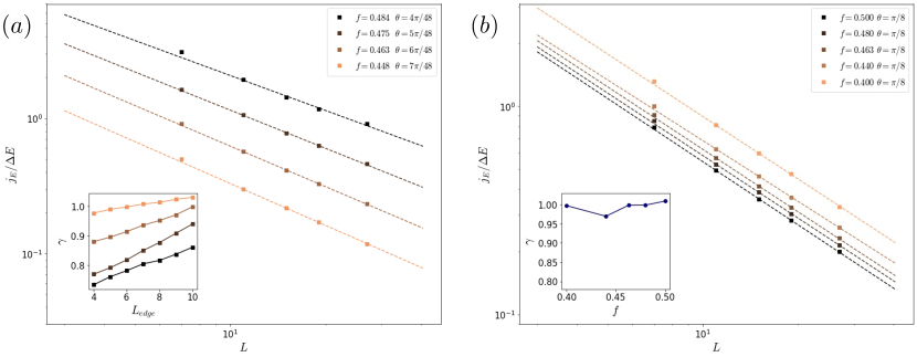
The outcomes of the scaled energy current $j_{E}/\Delta E$ under high-temperature conditions for both the gapless and gapped regimes are depicted in Fig. 3. Given that the model becomes non-integrable for non-zero chiralities, it is generally anticipated that the selected points in Fig. 1 would exhibit diffusive energy relaxation behavior. We start with the results on energy transport in the gapless regime. We choose specific values of $f$ and $\theta$ along the phase transition line, as detailed in Ref. [42]. In the calculation of the expectation values used for estimating transport coefficients, we account for the impact of driving and other boundary effects by excluding a total of $L_{\text{edge}}=10$ sites at each boundary. Among our chosen points, the influence of finite-size effects from the boundaries is relatively modest for the two cases with larger $\theta$ values. In these instances, we observe the anticipated diffusive transport behavior, with a scaling exponent $\gamma$ closely aligned with the expected value of 1, accompanied by a small uncertainty of approximately $\pm 0.03$. Conversely, the remaining two points with smaller $\theta$ values exhibit signs of superdiffusive transport, characterized by scaling exponents around the range of 0.8 to 0.9.

Given our anticipation of normal diffusive transport in cases where $T_{S}\gg J$ and the expected preservation of symmetrical properties, we proceed to examine how finite-size effects impact the scaling exponent $\gamma$ by systematically altering the number of sites excluded at the boundaries, denoted as $L_{\text{edge}}$. The inset in Fig. 3 (a) emphasizes the gradual rise of $\gamma$ as the bulk system size becomes more confined to a smaller number of central sites. While not a precise solution, this qualitative examination indicates that strong finite effects tend to exhibit the superdiffusivity. In general, we observe that the transport coefficients become challenging to compute as we approach the achiral model ($\theta\rightarrow 0$). Specifically, both the energy gradient $\Delta E$ and the energy current $j_{E}$ become exceedingly small in this region, preventing the transport coefficients from converging within the constraints of moderate simulation parameters.

Next, we delve into the analysis of energy transport within the gapped phases of the model. To explore potential variations in transport properties across the direct phase transition line, we focus on a specific point $(f=0.463,\theta=\pi/8)$, along with two additional points sharing the same $\theta$ value from both the disordered and $\mathbb{Z}_{3}$ ordered phases. This particular point demonstrates better convergence compared to smaller $\theta$ values and remains sufficiently distant from the intermediate incommensurate phase. Our investigations confirm the prevalence of diffusive energy transport across all the selected points, as depicted in Fig. 3 (b). Thus, it appears that the model’s transport behavior remains robust, seemingly unaffected by the low-temperature physics.

We have also extended our method to investigate scenarios where the gap size is comparable to the energy scale ($\Delta\sim J$). In such cases, the non-integrable model with a larger gap generally exhibits a shorter convergence time [75], although obtaining a reliable NESS in the large gap regime might be influenced by other factors. Similar to the situation with small $\theta$ values, we observe that the scaling exponent $\gamma$ (data not shown) gradually converges towards the normal diffusive value. However, the increasing trend of $\gamma$ is considerably smaller than 1, indicating that convergence of the NESS is affected by other factors, for example, difficulties estimating the gradient of energy and potential small gaps in the Liouvillian. Furthermore, it is noteworthy that the trace distance $K(\rho_{\text{NESS}},\rho(T_{S}))$ is primarily influenced by $T_{S}$. While a relatively lower $K(\rho_{\text{NESS}},\rho(T_{S}))$ doesn’t necessarily ensure the complete reliability of the NESS, it remains a critical criterion for assessing the accuracy of the calculated transport coefficients, considering the computational complexity involved.

Figure 4: (a) The scaled energy current $j_{E}/\Delta E$ at various bath temperatures is described in relation to the system size $L$, derived from the NESS results for the parameters $(f=0.463,\theta=\pi/8)$. The dashed lines illustrate the fitting according to the generalized Fourier’s law $j_{E}/\Delta E=-D/L^{\gamma}$ with $L_{\text{edge}}=10$. Inset provides a representation of the scaling exponent $\gamma$ extracted as a function of $f$. (b) The obtained diffusion constant $D$ from the generalized Fourier’s law is shown as a function of the reciprocal of the system’s temperature $T_{S}$ for two different bath sizes. The dashed line represents the best-fit power series curve expressed in Eq. (18). The inset plot illustrates the relationship between $T_{S}$ and $T_{B}$.

IV.2 Transport Coefficients at Lower Temperatures

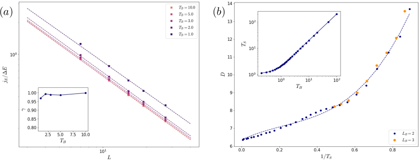
Now, we proceed to the study of energy transport at various temperatures using the same parameter point as in the slightly gapped regime analysis ($(f=0.463,\theta=\pi/8)$). The bath temperature is varied within the range of $0.5\leq T_{B}\leq 100$, covering high temperature all the way down to just below the scale of $J$. The scaled energy currents exhibit a proportional relationship with the inverse of the system size within this temperature range, as shown in Fig. 4 (a). This result indicates that diffusive energy transport persists even at temperatures comparable to the energy scale. Here, the trace distance $K$ serves as an indicator of the transport simulation’s performance, reflecting the deviation between the NESS expectation values and the thermal state. For higher temperatures, we observe $K\sim 10^{-3}$, whereas as we approach lower temperatures, the quality of $K$ deteriorates. As a result, we confine our investigation to temperatures where $K\sim 10^{-1}$ between the steady state and the thermal state, especially for the most challenging simulation scenarios.

Through our thermometry scheme, we observe a linear relationship between the effective system temperature $T_{S}$ and the bath temperature $T_{B}$ up to around $T_{B}\sim 1$. (as seen in the inset of Fig.4 (b)). In contrast, as the temperature decreases to lower limits, we notice that the improvement in $T_{S}$ becomes non-linear and levels off to a nonzero value, which is on the same order of magnitude as the energy scale of the model, as discussed with a smaller system size in our earlier work (Ref.  [31]). While it’s possible that $T_{S}$ is influenced by implicit model parameters, we consider it to be a fundamental aspect of the simulation method. In our prior research, we also observed a connection between the resulting $T_{S}$ and the implementation of the bath. Specifically, employing a bath with weaker bath-system interactions and larger bath sizes seems to enable access to lower temperatures in our system. On the other hand, using a weaker bath can lead to a numerical instability akin to what we observed in the high-temperature transport simulation as $\theta$ approaches zero. In general, the relaxation time is associated with the spectral gap $\Delta_{\mathcal{L}}$ of the super-operator. For our non-integrable model in a boundary-driven setup, perturbation theories suggest that the spectral gap scales as $\Delta_{\mathcal{L}}\sim\Gamma g^{2}/L$ in the limit of $g,\gamma\rightarrow 0$ [76, 75, 77]. Consequently, the relaxation time also follows this scaling behavior. This implies that reducing the strength of bath-system interaction $g$ leads to a notable increase in the time required for the NESS to reliably converge. However, it turns out that this trade-off provides only a marginal advantage in improving the effective temperature for this specific model. Despite implementing a larger bath, similar convergence issues persist, and the relaxation time remains largely unaffected by the bath size. In light of this, we explore the application of the 3-site bath technique in the low-temperature regime, as illustrated in Fig. 4 (b). Notably, expanding the bath size primarily offers an enhancement in the trace distance. Specifically, the trace distance is slightly improved (by approximately $10\%$) for the 3-site bath calculation when compared to the 2-site bath, while the estimated diffusion constants exhibit consistent agreement between the two cases.

Using the approach of estimating local temperature, we acquire temperature-dependent diffusion constants for the model, as depicted in Fig. 4 (b). Given that the effective temperature remains significantly higher, making it reasonable to disregard any potential power-law modifications for the zero-temperature limit, we can maintain the assumption of diffusive energy transport within the low-temperature regime. At high temperatures, the diffusion constant converges to a constant value of approximately $D_{\infty}\approx 6.3$, exhibiting a notable resemblance to the spin-$1/2$ model outlined in Ref. [48]. Given the system’s gapless nature at the quantum critical point, the energy gap $\Delta$ holds no significance in relation to its transport properties. Independent of the gap size, a power-series expansion in terms of the inverse temperature is a suitable approach for describing transport in the high-to-intermediate-temperature range, as discussed in Ref.  [48]. This expansion is expressed as

$$D=D_{\infty}\left(1+\sum_{a\geq 1}\frac{c_{a}}{T^{a}}\right).$$ (18)

At these temperature levels, the power-series fitting curve with $a=3$ exhibits excellent agreement with numerical results, indicating that the energy transport of the model falls within the realm of intermediate temperatures. However, the increasing trend in the diffusivity at the lowest temperature we observed is not entirely clear. Given that the model lacks a gap, one could speculate that a new energy scale needs to be introduced to elucidate this trend within the semi-classical kinetic theory for gapped systems [78, 79, 48].

V Discussion

In this paper, we studied the finite temperature energy transport in the non-integrable $\mathbb{Z}_{3}$ chiral clock model by utilizing tensor network-based simulations of the open quantum system approach. Based on the notion of local temperature, the NESS’s effective temperature is evaluated using trace distance-based thermometry. Subsequently, transport characteristics of the model are derived from the NESS using the generalized Fourier’s law. In the high-temperature regime, we observe diffusive energy transport regardless of model parameters so long as we consider the non-integrable regime. This confirms our expectation that the low-temperature physics does not directly affect the high-temperature transport. Subsequently, we choose parameters corresponding to a quantum critical point at zero temperature to study the temperature dependence of transport coefficients. With modest computational resources, we are able to probe transport at lower temperatures comparable to the characteristic energy scale, $J$, of the model. The use of both $2-$ and $3-$site baths yields consistent outcomes in terms of extracting temperature-dependent diffusion constants at this specific point. Notably, the resulting diffusion constant at this point in the phase diagram aligns well with a power-series expansion in terms of inverse temperature.

By dedicating significantly larger computational resources, there is potential to delve into energy transport at even lower temperatures with the aspiration of approaching the intrinsic minimum temperature achievable by the boundary-driven setup. At much lower temperatures, it becomes intriguing to investigate the emergence of power-law behavior in the temperature dependence of the transport coefficients, which could serve as an indication of a quantum critical transport regime. Furthermore, exploring the potential correlation between the model’s transport properties and its chiralities (and consequently its symmetries) at low temperatures offers another compelling avenue for future exploration.

The exploration of these fascinating phenomena can be facilitated through carefully engineered reservoir configurations. In a previous study (Ref. [31]), a minimum attainable temperature for the gapless chiral clock model was suggested. An interesting avenue for future research could involve developing a comprehensive framework for designing optimized baths and dynamics, aiming to overcome this limitation. One possible approach to tackle this challenge involves approximating larger baths using the Product Spectrum Ansatz [80, 81] for designing dissipators, as larger baths often lead to improved thermalization. Another potential avenue is the design of unconventional baths [82], including those based on random energy models or random matrix models. These bath models tend to exhibit densely populated spectral densities, suggesting that they could lead to effective thermalization if they can be implemented at a considerably large scale. Additionally, exploring similar techniques with other quantum master equations, such as the Redfield equation, could also be considered.

Appendix A Details of Tensor Network Simulations

Figure 5: Typical convergence of the NESS for $L=32$, $\chi=200$ at the critical point ($\chi=200,f=0.463,\theta=\pi/8)$ at various bath temperatures. (a) Schmidt spectrum at the center of the chain. The best power-law fittings are presented with dashed lines. (b) Convergence of the scaled energy current as a function of bond dimension $\chi$.

Our main goal in this text is to investigate how the energy transport of the $\mathbb{Z}_{3}$ CCM is influenced by temperature variations. In this section, we take a closer look at the details of our tensor network calculations. For our finite temperature tensor network approach, we choose the vectorization approach to depict the density matrix [63] over the purification approach [83]. While this approach doesn’t necessarily preserve positivity, it generally offers a more effective way to represent an open quantum system setup compared to alternatives. Using this formalism, we introduce the finite temperature bath into the superoperator $L$, as outlined in Eq. 8.

In the context of the boundary driving setup and using the specified superoperators, we attain a non-equilibrium steady state by employing the TEBD algorithm on the vectorized density matrix [66, 67, 84]. The time evolution superoperator is represented as $U=e^{\mathcal{L}\delta t}$ and is discretized using the Suzuki-Trotter decomposition. The $2k-$th order Suzuki-Trotter decomposition of the time evolution operator $U^{(2k)}$ is defined by the following recurrence relation [85],

$$U^{(2)}(\delta t) =e^{\frac{\delta t}{2}\mathcal{L}_{N-1}}\cdots e^{\frac{\delta t}{2}\mathcal{L}_{1}},$$ (19)

$$U^{(2k)}(\delta t) =U^{(2k-2)}(u_{k}\delta t)^{2}U^{(2k-2)}((1-4u_{k})\delta t)U^{(2k-2)}(u_{k}\delta t)^{2},$$ (20)

where $u_{k}=1/(4-4^{1/(2k-1)})$. In our simulations, we opt for a second-order approximation and set the time step to $\delta t=0.05$. When applying the discretized time evolution operator, we introduce a cumulative error of order $\mathcal{O}(\delta t^{2k+1})$ into our final state and, consequently, its expectation values. Despite this, we observe that the error remains below $1\%$ within the parameters of our simulation.

An additional significant source of simulation error emerges from truncating the operator Hilbert space dimension of the density matrix. The extent of this truncation error is intricately linked to the operator space entanglement entropy of the NESS. To manage the computational complexity of the simulation, we utilize the standard Schmidt value truncation. In this approach, the Schmidt decomposition of the density matrix into two subsystems, denoted as $A$ and $B$, is expressed as [86]:

$$\rho=\sum_{m}\sqrt{\lambda_{m}}\rho_{m}^{A}\otimes\rho_{m}^{B}.$$ (21)

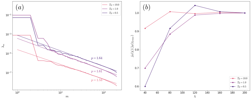
Subsequently, the truncation error is evaluated as the sum of truncated Schmidt values, expressed as $\sum_{m>\chi}\lambda_{m}$. The canonical representation of MPS conveniently grants direct access to the spectrum of Schmidt values [11]. In our simulations, we notice a characteristic asymptotic power-law decay [10], denoted as $\lambda_{m}\sim m^{-p}$ (refer to Fig. 5 (a)), which holds true for all simulation parameters. Hence, we believe that the non-equilibrium state will exhibit an efficient representation in terms of tensor networks even at low temperatures and extended local Hilbert space.

The combination of the cumulative Suzuki-Trotter expansion error and the truncated Hilbert space error introduces an imperfect representation of $\rho_{\text{NESS}}$ as a tensor network. This inherent instability manifests as minor fluctuations in the expectation values, persisting even at later stages of the simulation. To estimate the most probable physical outcome, we take an average of our expectation values over approximately $10^{3}$ Trotter steps, considering the most challenging simulation in our study.

Typically, opting for the initial state as an infinite temperature state, the dynamics encounters an upsurging entanglement entropy in the early stages, reaching saturation in later times. To ensure a good approximation at each time domain as the density matrix evolves, we employ varying bond dimensions. Initially, we start with a large bond dimension, $\chi=200$, during the early stages, and then reduce $\chi$ to 81 for intermediate times where the entanglement entropy begins to saturate while the expectation values continue evolving. Subsequently, at late times, we increase the bond dimension back to $\chi=200$ to fine-tune our solution. We consistently verify the convergence of NESS observables with the bond dimension and find $\chi=200$ to be sufficient within our range of study. The convergence of the NESS expectation value, as illustrated in Fig. 5, confirms that the NESS energy current improves with a larger $\chi$, aligning with the power-law decay of the Schmidt value spectrum closely tied to the estimated error order [10].

Similar to chaotic spin-$1/2$ systems, our system converges to a unique NESS as a consequence of its dynamics [55]. When initializing the system with various states $\rho(0)$, we verify that the resulting state converges to the same NESS, with differences being negligible and attributed to cumulative errors and late-time fluctuations. The uniqueness of this NESS enables us to employ a temperature annealing strategy for lower temperature simulations, in which the relaxation times to reach the NESS are significantly extended. The primary computational workload arises from the gradual evolution during the mid-later stages. However, the early time evolution from an infinite temperature state can be bypassed by initiating the process with a slightly higher temperature NESS to attain the subsequent lower temperature NESS.