A novel method for holographic transport
Abstract
We introduce a novel and effective method to compute transport coefficients in strongly interacting plasma states in holographic QFTs. Our method is based on relating the IR limit of fluctuations on a gravitational background to its variations providing a previously overlooked connection between boundary and near horizon data. We use this method to derive analytic formulas for the viscosities of an anisotropic plasma state in the presence of an external magnetic field or another isotropy breaking external source. We then apply our findings to holographic QCD.
I Introduction
Gauge-gravity duality Maldacena (1998); Gubser et al. (1998); Witten (1998) has emerged as an essential tool in characterizing transport in strongly interacting many-body systems such as the quark-gluon plasma and dense quark matter produced in heavy ion collisions and neutron star mergers, as well as condensed matter such as high- superconductors and resonantly interacting ultra-cold atoms. The celebrated holographic prediction for the shear viscosity-entropy ratio Policastro et al. (2001, 2002); Kovtun et al. (2003) provides a very good estimate for the quark-gluon plasma — see for example Nijs et al. (2021a, b); Everett et al. (2021a, b). Among other successful predictions of the holographic approach are the bulk viscosity of the quark-gluon plasma Benincasa et al. (2006); Buchel (2008); Buchel and Liu (2004); Buchel (2005); Gubser et al. (2008); Eling and Oz (2011); Buchel et al. (2011), electric and thermal conductivities Hartnoll (2009), chiral anomalous transport Erdmenger et al. (2009); Gynther et al. (2011) and Hall viscosity of magnetized plasmas Hoyos et al. (2019).
Standard holographic computation of a transport coefficient involves determining response of plasma to perturbation by solving for the fluctuation created by this perturbation on the boundary and falling in the horizon of the dual blackhole. In fact, this relation between transport and blackhole horizons predates the gauge-gravity duality. The membrane paradigm Price and Thorne (1986); Thorne et al. (1986) proposed to reformulate Einstein’s equations near horizon in terms of hydrodynamics of a putative fluid characterized by transport coefficients. This idea was later reified in the context of holography using different approaches Iqbal and Liu (2009); Crossley et al. (2017); Bhattacharyya et al. (2008); de Boer et al. (2015); Eling and Oz (2010); Liu et al. (2017). However, only in special “universal” cases e.g. shear viscosity and electric conductivity of an isotropic fluid— which are dual to massless helicity-2 and helicity-1 fluctuations — transport coefficients can be expressed solely in terms of horizon data. This is because response is read off from the subleading term near the boundary which can be mapped to horizon data only for such massless fluctuations 111An exception is Eling and Oz (2011) where an analytic formula for the bulk viscosity in terms of horizon data was provided using the Raychaudhuri equation Raychaudhuri (1955). However, this approach is only applicable to dissipative transport as it is based on reformulating Einstein’s equations as divergence of the entropy current to which only dissipative transport contributes.. The situation is further complicated by isotropy breaking external fields, e.g. a magnetic field, that are present in all the aforementioned examples.
In this paper we introduce a novel means to study holographic transport which allows for reading off both universal and non-universal coefficients directly from the horizon. The fact that transport coefficients are obtained from the IR limit of bulk fluctuations suggest that they are intimately related to variations in the background geometry. We flesh this idea out and utilize it to provide a novel and effective method to compute these quantities.
II The method
Our basic idea is to relate limit of bulk fluctuations — the standard holographic prescription to compute transport coefficients — to variations of parameters of the holographic background such as temperature and charge. Below is a demonstration in the case of bulk viscosity, , in an isotropic background. The minimal holographic set-up Gursoy and Kiritsis (2008); Gursoy et al. (2008a) that is dual to a non-conformal theory with non-trivial is a black-brane
| (1) |
coupled to scalar field and a gauge field with field strength with an action,
| (2) |
where the potential is chosen such that the metric is asymptotically Anti-de-Sitter near the boundary and we keep the gauge field Lagrangian unspecified. Thermodynamics and transport of the dual thermal field theory has been studied in detail in Gursoy et al. (2009a); Charmousis et al. (2010) and Gursoy et al. (2009b). We first review the standard holographic computation Gubser et al. (2008); Gursoy et al. (2009b) of bulk viscosity. This follows from fluctuating the metric 222We choose a gauge to set fluctuations of to zero. as , with
| (3a) | ||||
| (3b) | ||||
| (3c) | ||||
| (3d) | ||||
Corresponding fluctuation equations, that are obtained from (2), turn out to have a nested structure Gubser et al. (2008) which determines the solution completely in terms of . Assuming time dependence of the form etc. and imposing infalling boundary conditions at the horizon, one obtains in the limit
| (4) |
where is the entropy density, subscript denotes horizon value, and is the horizon value of the fluctuation in the limit obtained by numerically solving the fluctuation equation with the boundary conditions
| (5) |
These boundary conditions follows from the fact that the Kubo formula connects bulk viscosity to the correlator of the energy momentum tensor with spatial indices.
We will now show that Eq. (4), can be rewritten in terms of variations of background fields. We consider the charge neutral case for simplicity, the generalization to the charged case being straightforward. We first relate fluctuations to variations of the background, which leads to
| (6a) | ||||
| (6b) | ||||
| (6c) | ||||
In Eq. (6) we used diffeomorphism symmetry to set the fluctuation of the dilaton to zero to remain consistent with the standard computation outlined above. Now, as with the equivalence of active and passive transformations in classical mechanics, we can create the same situation as fluctuation added on a fixed background instead by varying the background so as to subtract this fluctuation. This requires finding the right symmetry transformations to produce new backgrounds from the given one in order to obtain the desired boundary values for the fluctuations. Symmetries of a generic background (1) are Gursoy et al. (2008b, 2009a):
| (7a) | ||||
| (7b) | ||||
where parametrize independent infinitesimal transformations. Now, inverting (6), adding the symmetry transformations (7) with and judiciously chosen to reproduce (5), and expanding near the horizon, one finds
| (8) |
with is an arbitrary constant which could be set to zero by choosing appropriately and which cancels below. One finally obtains for the total variation of the background functions
| (9) |
where we used and (8) to determine the variation of horizon. Note that here and denote the variations of the boundary values of the fields, whereas , , and are the variations of the functions evaluated at the horizon. Finally, to express (4) in terms of physical quantities, we note that . Therefore, we can write
| (10) |
Employing Eq. (4) we finally obtain
| (11) |
This result coincides with the formula initially derived in Eling and Oz (2011), using positivity of entropy production near horizon, which was numerically shown to be equivalent to Eq. (4) in Ref. Buchel et al. (2011). Our derivation does not use entropy arguments, and relates directly to horizon data .
III Anisotropic transport
To apply our method to the more complex and unexplored case of transport in anisotropic fluids, we consider an external (non-dynamical) magnetic field 333We also assume parity and time-reversal symmetry. which decomposes the leading order dissipative correction to stress tensor as Hernandez and Kovtun (2017); Armas and Jain (2019)
| (12) | ||||
where we define the projectors
| (13) | ||||
Our goal is to compute the anisotropic transport coefficients that appear in (12) using holography. Magnetic field is holographically realized by choosing the bulk gauge field in (2) as
| (14) |
Accordingly, we should introduce an anisotropy function in the metric ansatz as
| (15) |
The shear viscosities and were computed in Ref. Jain et al. (2015) and it was found that
| (16) |
See Landsteiner et al. (2016); Davison et al. (2022); Bhattacharyya and Roychowdhury (2015) for some recent holographic studies of transport in anisotropic thermal states.
III.1 Anisotropic bulk viscosities from fluctuations
Aiming at generalizing Eq. (4) to the anisotropic case we consider metric fluctuations
| (17a) | ||||
| (17b) | ||||
| (17c) | ||||
| (17d) | ||||
| (17e) | ||||
We see that we now have two spatial scalar fluctuations and , which do not have a decoupled fluctuation equations, unlike was the case for the isotropic . We apply the approach based on conserved graviton flux between the boundary and the horizon, introduced in Gubser et al. (2008) and generalized to multiple fluctuations in Kaminski et al. (2010). We only sketch the most relevant points below, see Demircik et al. (2024) for details. We first construct linear combination of fluctuations which decouple from each other near the horizon. These are
| (18a) | ||||
| (18b) | ||||
Assuming harmonic time dependence so that , we find
| (19) |
where are coefficients that depend on the background fields and are subleading near the horizon. We now have two fluctuations near horizon that are coupled near the boundary. We can label the linearly independent boundary conditions also by index which leads to a 22 matrix whose solution near the horizon and in the limit we denote by ; this is analogous to in the previous section. Following Gubser et al. (2008), Kaminski et al. (2010) we obtain the retarded Green’s functions to leading order in in terms of the flux of gravitons at the horizon as
where the expressions for reflect the form of in (19). One finds from Eq. (12), see Hernandez and Kovtun (2017), that
| (20a) | ||||
| (20b) | ||||
| (20c) | ||||
III.2 Anisotropic bulk viscosities from variations
We now apply our method to express Eq. (20) in horizon data. As in (6) fluctuations are expressed in terms of background variations as 444We again use the gauge where the fluctuation of the dilaton vanishes.
| (21a) | ||||
| (21b) | ||||
| (21c) | ||||
| (21d) | ||||
Following the same steps as in the isotropic case discussed above we now work out the symmetry transformations of the background to cancel the boundary sources. There is an additional symmetry under which the new background functions and transform as and while transformations of , and remain as in (7). Now, in addition to (5) we also have the boundary values of either of to cancel. We use the extra symmetry parameter to cancel them. Inverting (21), adding the symmetry transformations with , chosen to cancel the fluctuations on the boundary one expresses variations of the background at the horizon in terms . We spare the reader from these rather long formulas — see Demircik et al. (2024) for details — and instead present the final relations between and complete background variations i.e. etc. where is read off from exactly as above
| (22a) | ||||
| (22b) | ||||
| (22c) | ||||
| (22d) | ||||
Substitution of Eq. (22) into Eq. (20) leads to our final expressions for the magnetically induced anisotropic bulk viscosities
| (23a) | ||||
| (23b) | ||||
| (23c) | ||||
Note that these expressions satisfy the constraints that arise from positivity of local entropy production
| (24) |
that were obtained in Hernandez and Kovtun (2017); Armas and Jain (2019). In our accompanying paper Demircik et al. (2024), we derived the same results independently using the Raychaudhuri equation and positivity of entropy production by extending Eling and Oz (2011) to anisotropic horizons.
IV Application to QCD
We finally apply our end result for anisotropic viscosities (23) in a realistic holographic QCD model. In doing so we shall also validate these expressions by numerically comparing the results obtained via the background variation method and the standard fluctuation analysis (20). To this end, we employ V-QCD Järvinen and Kiritsis (2012), a bottom-up effective model that incorporates a relatively extensive set of parameters meticulously adjusted to match with experimental QCD data, lattice QCD findings, and perturbative QCD predictions. This widely accepted and successful model serves as a valuable tool for describing both the different phases of QCD and investigating various phenomena at finite-temperature Alho et al. (2013); Areán et al. (2013); Jokela et al. (2019); Alho et al. (2015); Iatrakis et al. (2017), finite-density Alho et al. (2014); Ishii et al. (2019); Jarvinen (2015); Ecker et al. (2020); Hoyos et al. (2020); Demircik et al. (2022, 2021); Hoyos et al. (2022); Tootle et al. (2022); Cruz Rojas et al. (2023), finite-magnetic-field Drwenski et al. (2016); Demircik and Gursoy (2017); Gürsoy et al. (2017, 2019, 2021) and in the presence of anisotropies Giataganas et al. (2018). In the case of V-QCD, the matter Lagrangian in (2) takes the Dirac-Born-Infeld form Bigazzi et al. (2005); Casero et al. (2007). For detailed information on V-QCD, we refer to Järvinen and Kiritsis (2012) and the comprehensive review Järvinen (2022).
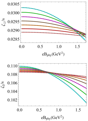
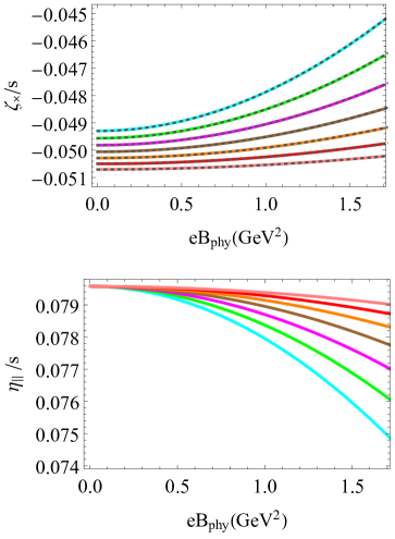
Sparing the details of the numerical computation to our accompanying paper Demircik et al. (2024), we present our results depicting temperature and magnetic field dependence of anisotropic viscosities in Fig. 1. For completeness we also plot which we compute using Eq. (16). Solid colored curves are obtained using the fluctuation analysis whereas the dotted gray curves follow from (23) and we see perfect agreement. As additional consistency checks on our numerics, we verified that the Onsager relations Hernandez and Kovtun (2017) are satisfied, and showed that our results are consistent in the limit of with earlier literature Hernandez and Kovtun (2017); Buchel et al. (2011).
V Discussion
We observe in Fig. 1 that both the magnetic field and temperature dependence of bulk viscosities are overall very mild. This implies that these transport coefficients can approximately be treated as constant in numerical hydrodynamic simulations. We find that while is larger than the universal value () of the shear viscosity-entropy ratio, whereas and are smaller but still significant.
Analytic expressions like (23) and (16) are extremely useful in deriving universal relations among transport coefficients. For example, one can easily prove a universal bound using (16) and Einstein equations Demircik et al. (2024). One can also compute electric conductivities () perpendicular (parallel) to in the absence of background charge. One then finds another intriguing universal relation Demircik et al. (2024):
A similar relation was already observed in Landsteiner et al. (2016). One wonders whether these universal relations extend to the domain of finite ’t Hooft coupling. To explore this one will need to extend our analysis to include higher derivative corrections to Einstein’s gravity.
VI Acknowledgments
We are grateful to Niko Jokela, Govert Nijs and Francisco Peña-Benitez for discussions. This work was supported, in part by the Netherlands Organisation for Scientific Research (NWO) under the VICI grant VI.C.202.104. T.D. acknowledges the support of the Narodowe Centrum Nauki (NCN) Sonata Bis Grant No. 2019/34/E/ST3/00405. M. J. has been supported by an appointment to the JRG Program at the APCTP through the Science and Technology Promotion Fund and Lottery Fund of the Korean Government. M. J. has also been supported by the Korean Local Governments – Gyeongsangbuk-do Province and Pohang City – and by the National Research Foundation of Korea (NRF) funded by the Korean government (MSIT) (grant number 2021R1A2C1010834).
References
- Maldacena (1998) J. M. Maldacena, Adv. Theor. Math. Phys. 2, 231 (1998), arXiv:hep-th/9711200 .
- Gubser et al. (1998) S. S. Gubser, I. R. Klebanov, and A. M. Polyakov, Phys. Lett. B 428, 105 (1998), arXiv:hep-th/9802109 .
- Witten (1998) E. Witten, Adv. Theor. Math. Phys. 2, 253 (1998), arXiv:hep-th/9802150 .
- Policastro et al. (2001) G. Policastro, D. T. Son, and A. O. Starinets, Phys. Rev. Lett. 87, 081601 (2001), arXiv:hep-th/0104066 .
- Policastro et al. (2002) G. Policastro, D. T. Son, and A. O. Starinets, JHEP 09, 043 (2002), arXiv:hep-th/0205052 .
- Kovtun et al. (2003) P. Kovtun, D. T. Son, and A. O. Starinets, JHEP 10, 064 (2003), arXiv:hep-th/0309213 .
- Nijs et al. (2021a) G. Nijs, W. van der Schee, U. Gürsoy, and R. Snellings, Phys. Rev. Lett. 126, 202301 (2021a), arXiv:2010.15130 [nucl-th] .
- Nijs et al. (2021b) G. Nijs, W. van der Schee, U. Gürsoy, and R. Snellings, Phys. Rev. C 103, 054909 (2021b), arXiv:2010.15134 [nucl-th] .
- Everett et al. (2021a) D. Everett et al. (JETSCAPE), Phys. Rev. Lett. 126, 242301 (2021a), arXiv:2010.03928 [hep-ph] .
- Everett et al. (2021b) D. Everett et al. (JETSCAPE), Phys. Rev. C 103, 054904 (2021b), arXiv:2011.01430 [hep-ph] .
- Benincasa et al. (2006) P. Benincasa, A. Buchel, and A. O. Starinets, Nucl. Phys. B 733, 160 (2006), arXiv:hep-th/0507026 .
- Buchel (2008) A. Buchel, Phys. Lett. B 663, 286 (2008), arXiv:0708.3459 [hep-th] .
- Buchel and Liu (2004) A. Buchel and J. T. Liu, Phys. Rev. Lett. 93, 090602 (2004), arXiv:hep-th/0311175 .
- Buchel (2005) A. Buchel, Phys. Lett. B 609, 392 (2005), arXiv:hep-th/0408095 .
- Gubser et al. (2008) S. S. Gubser, S. S. Pufu, and F. D. Rocha, JHEP 08, 085 (2008), arXiv:0806.0407 [hep-th] .
- Eling and Oz (2011) C. Eling and Y. Oz, JHEP 06, 007 (2011), arXiv:1103.1657 [hep-th] .
- Buchel et al. (2011) A. Buchel, U. Gursoy, and E. Kiritsis, JHEP 09, 095 (2011), arXiv:1104.2058 [hep-th] .
- Hartnoll (2009) S. A. Hartnoll, Class. Quant. Grav. 26, 224002 (2009), arXiv:0903.3246 [hep-th] .
- Erdmenger et al. (2009) J. Erdmenger, M. Haack, M. Kaminski, and A. Yarom, JHEP 01, 055 (2009), arXiv:0809.2488 [hep-th] .
- Gynther et al. (2011) A. Gynther, K. Landsteiner, F. Pena-Benitez, and A. Rebhan, JHEP 02, 110 (2011), arXiv:1005.2587 [hep-th] .
- Hoyos et al. (2019) C. Hoyos, F. Peña-Benitez, and P. Witkowski, Journal of High Energy Physics 2019, 146 (2019).
- Price and Thorne (1986) R. H. Price and K. S. Thorne, Phys. Rev. D 33, 915 (1986).
- Thorne et al. (1986) K. S. Thorne, R. H. Price, and D. A. Macdonald, eds., BLACK HOLES: THE MEMBRANE PARADIGM (1986).
- Iqbal and Liu (2009) N. Iqbal and H. Liu, Phys. Rev. D 79, 025023 (2009), arXiv:0809.3808 [hep-th] .
- Crossley et al. (2017) M. Crossley, P. Glorioso, and H. Liu, JHEP 09, 095 (2017), arXiv:1511.03646 [hep-th] .
- Bhattacharyya et al. (2008) S. Bhattacharyya, V. E. Hubeny, S. Minwalla, and M. Rangamani, JHEP 02, 045 (2008), arXiv:0712.2456 [hep-th] .
- de Boer et al. (2015) J. de Boer, M. P. Heller, and N. Pinzani-Fokeeva, JHEP 08, 086 (2015), arXiv:1504.07616 [hep-th] .
- Eling and Oz (2010) C. Eling and Y. Oz, JHEP 02, 069 (2010), arXiv:0906.4999 [hep-th] .
- Liu et al. (2017) H.-S. Liu, H. Lu, and C. N. Pope, JHEP 09, 146 (2017), arXiv:1708.02329 [hep-th] .
- Note (1) An exception is Eling and Oz (2011) where an analytic formula for the bulk viscosity in terms of horizon data was provided using the Raychaudhuri equation Raychaudhuri (1955). However, this approach is only applicable to dissipative transport as it is based on reformulating Einstein’s equations as divergence of the entropy current to which only dissipative transport contributes.
- Gursoy and Kiritsis (2008) U. Gursoy and E. Kiritsis, JHEP 02, 032 (2008), arXiv:0707.1324 [hep-th] .
- Gursoy et al. (2008a) U. Gursoy, E. Kiritsis, and F. Nitti, JHEP 02, 019 (2008a), arXiv:0707.1349 [hep-th] .
- Gursoy et al. (2009a) U. Gursoy, E. Kiritsis, L. Mazzanti, and F. Nitti, JHEP 05, 033 (2009a), arXiv:0812.0792 [hep-th] .
- Charmousis et al. (2010) C. Charmousis, B. Gouteraux, B. S. Kim, E. Kiritsis, and R. Meyer, JHEP 11, 151 (2010), arXiv:1005.4690 [hep-th] .
- Gursoy et al. (2009b) U. Gursoy, E. Kiritsis, G. Michalogiorgakis, and F. Nitti, JHEP 12, 056 (2009b), arXiv:0906.1890 [hep-ph] .
- Note (2) We choose a gauge to set fluctuations of to zero.
- Gursoy et al. (2008b) U. Gursoy, E. Kiritsis, L. Mazzanti, and F. Nitti, Phys. Rev. Lett. 101, 181601 (2008b), arXiv:0804.0899 [hep-th] .
- Note (3) We also assume parity and time-reversal symmetry.
- Hernandez and Kovtun (2017) J. Hernandez and P. Kovtun, JHEP 05, 001 (2017), arXiv:1703.08757 [hep-th] .
- Armas and Jain (2019) J. Armas and A. Jain, Physical Review Letters 122 (2019), 10.1103/physrevlett.122.141603.
- Jain et al. (2015) S. Jain, R. Samanta, and S. P. Trivedi, JHEP 10, 028 (2015), arXiv:1506.01899 [hep-th] .
- Landsteiner et al. (2016) K. Landsteiner, Y. Liu, and Y.-W. Sun, Physical Review Letters 117 (2016), 10.1103/physrevlett.117.081604.
- Davison et al. (2022) R. A. Davison, B. Goutéraux, and E. Mefford, (2022), arXiv:2210.14802 [hep-th] .
- Bhattacharyya and Roychowdhury (2015) A. Bhattacharyya and D. Roychowdhury, JHEP 03, 063 (2015), arXiv:1410.3222 [hep-th] .
- Kaminski et al. (2010) M. Kaminski, K. Landsteiner, J. Mas, J. P. Shock, and J. Tarrio, JHEP 02, 021 (2010), arXiv:0911.3610 [hep-th] .
- Demircik et al. (2024) T. Demircik, D. Gallegos, U. Gürsoy, M. Järvinen, and R. Lier, (2024), arXiv:2402.12224 [hep-th] .
- Note (4) We again use the gauge where the fluctuation of the dilaton vanishes.
- Järvinen and Kiritsis (2012) M. Järvinen and E. Kiritsis, JHEP 03, 002 (2012), arXiv:1112.1261 [hep-ph] .
- Alho et al. (2013) T. Alho, M. Järvinen, K. Kajantie, E. Kiritsis, and K. Tuominen, JHEP 01, 093 (2013), arXiv:1210.4516 [hep-ph] .
- Areán et al. (2013) D. Areán, I. Iatrakis, M. Järvinen, and E. Kiritsis, JHEP 11, 068 (2013), arXiv:1309.2286 [hep-ph] .
- Jokela et al. (2019) N. Jokela, M. Järvinen, and J. Remes, JHEP 03, 041 (2019), arXiv:1809.07770 [hep-ph] .
- Alho et al. (2015) T. Alho, M. Jarvinen, K. Kajantie, E. Kiritsis, and K. Tuominen, Phys. Rev. D 91, 055017 (2015), arXiv:1501.06379 [hep-ph] .
- Iatrakis et al. (2017) I. Iatrakis, E. Kiritsis, C. Shen, and D.-L. Yang, JHEP 04, 035 (2017), arXiv:1609.07208 [hep-ph] .
- Alho et al. (2014) T. Alho, M. Järvinen, K. Kajantie, E. Kiritsis, C. Rosen, and K. Tuominen, JHEP 04, 124 (2014), [Erratum: JHEP 02, 033 (2015)], arXiv:1312.5199 [hep-ph] .
- Ishii et al. (2019) T. Ishii, M. Järvinen, and G. Nijs, JHEP 07, 003 (2019), arXiv:1903.06169 [hep-ph] .
- Jarvinen (2015) M. Jarvinen, JHEP 07, 033 (2015), arXiv:1501.07272 [hep-ph] .
- Ecker et al. (2020) C. Ecker, M. Järvinen, G. Nijs, and W. van der Schee, Phys. Rev. D 101, 103006 (2020), arXiv:1908.03213 [astro-ph.HE] .
- Hoyos et al. (2020) C. Hoyos, N. Jokela, M. Jarvinen, J. G. Subils, J. Tarrio, and A. Vuorinen, Phys. Rev. Lett. 125, 241601 (2020), arXiv:2005.14205 [hep-th] .
- Demircik et al. (2022) T. Demircik, C. Ecker, and M. Järvinen, Phys. Rev. X 12, 041012 (2022), arXiv:2112.12157 [hep-ph] .
- Demircik et al. (2021) T. Demircik, C. Ecker, and M. Järvinen, Astrophys. J. Lett. 907, L37 (2021), arXiv:2009.10731 [astro-ph.HE] .
- Hoyos et al. (2022) C. Hoyos, N. Jokela, M. Järvinen, J. G. Subils, J. Tarrí o, and A. Vuorinen, Physical Review D 105 (2022), 10.1103/physrevd.105.066014.
- Tootle et al. (2022) S. Tootle, C. Ecker, K. Topolski, T. Demircik, M. Järvinen, and L. Rezzolla, SciPost Phys. 13, 109 (2022), arXiv:2205.05691 [astro-ph.HE] .
- Cruz Rojas et al. (2023) J. Cruz Rojas, T. Demircik, and M. Järvinen, Symmetry 15, 331 (2023), arXiv:2301.03173 [hep-th] .
- Drwenski et al. (2016) T. Drwenski, U. Gursoy, and I. Iatrakis, JHEP 12, 049 (2016), arXiv:1506.01350 [hep-th] .
- Demircik and Gursoy (2017) T. Demircik and U. Gursoy, Nucl. Phys. B 919, 384 (2017), arXiv:1605.08118 [hep-th] .
- Gürsoy et al. (2017) U. Gürsoy, I. Iatrakis, M. Järvinen, and G. Nijs, JHEP 03, 053 (2017), arXiv:1611.06339 [hep-th] .
- Gürsoy et al. (2019) U. Gürsoy, M. Järvinen, G. Nijs, and J. F. Pedraza, JHEP 04, 071 (2019), [Erratum: JHEP 09, 059 (2020)], arXiv:1811.11724 [hep-th] .
- Gürsoy et al. (2021) U. Gürsoy, M. Järvinen, G. Nijs, and J. F. Pedraza, JHEP 03, 180 (2021), arXiv:2011.09474 [hep-th] .
- Giataganas et al. (2018) D. Giataganas, U. Gürsoy, and J. F. Pedraza, Phys. Rev. Lett. 121, 121601 (2018), arXiv:1708.05691 [hep-th] .
- Bigazzi et al. (2005) F. Bigazzi, R. Casero, A. L. Cotrone, E. Kiritsis, and A. Paredes, JHEP 10, 012 (2005), arXiv:hep-th/0505140 .
- Casero et al. (2007) R. Casero, E. Kiritsis, and A. Paredes, Nucl. Phys. B 787, 98 (2007), arXiv:hep-th/0702155 .
- Järvinen (2022) M. Järvinen, Eur. Phys. J. C 82, 282 (2022), arXiv:2110.08281 [hep-ph] .
- Jokela et al. (2021) N. Jokela, M. Järvinen, G. Nijs, and J. Remes, Phys. Rev. D 103, 086004 (2021), arXiv:2006.01141 [hep-ph] .
- Raychaudhuri (1955) A. Raychaudhuri, Phys. Rev. 98, 1123 (1955).