Complex orders and chirality in the classical Kitaev-$\bm{\Gamma}$ model

Abstract

It is well-recognized that the low-energy physics of many Kitaev materials is governed by two dominant energy scales, the Ising-like Kitaev coupling $K$ and the symmetric off-diagonal $\Gamma$ coupling. An understanding of the interplay between these two scales is therefore the natural starting point toward a quantitative description that includes sub-dominant perturbations that are inevitably present in real materials. The present study focuses on the classical $K$-$\Gamma$ model on the honeycomb lattice, with a specific emphasis on the region $K\!<\!0$ and $\Gamma\!>\!0$, which is the most relevant for the available materials and which remains enigmatic in both quantum and classical limits, despite much effort. We employ large-scale Monte Carlo simulations on specially designed finite-size clusters and unravel the presence of a complex multi-sublattice magnetic orders in a wide region of the phase diagram, whose structure is characterized in detail. We show that this order can be quantified in terms of a coarse-grained scalar-chirality order, featuring a counter-rotating modulation on the two spin sublattices. We also provide a comparison to previous studies and discuss the impact of quantum fluctuations on the phase diagram.

I Introduction

Mott insulators with a strong spin-orbit coupling (SOC) have been the subject of a significant research interest in the past decade [1, 2, 3, 4, 5, 6, 7, 8, 9]. In these systems, an interplay of SOC with the crystal fields and strong electron-electron interactions yields anisotropic bond-dependent exchange interactions between low-energy spin degrees of freedom [9]. Most notably, a lot of effort has been devoted to the experimental investigation of the 4$d$ and 5$d$ materials, such as, e.g., A₂IrO₃ (A=Na, Li) [10, 11, 12, 13, 14, 15] and $\alpha$-RuCl₃ [16, 17, 18], with the goal of finding candidates to realize the Kitaev spin liquid [19], a highly exotic quantum phase of matter. This phase is characterized by fractionalized excitations, non-Abelian anyons, and topological properties that make it of significant interest to physicists. The Kitaev coupling, as originally introduced by Kitaev in 2006 [19], is indeed the dominant microscopic interaction in all these materials, hence the term ‘Kitaev materials’  [7]. However, despite the dominance of the Kitaev coupling, most of these materials exhibit magnetic ordering at sufficiently low temperatures [5, 6, 7, 8], indicating the presence of additional interactions in the system.

Studies suggest that a minimal nearest-neighbor (NN) model that effectively describes Kitaev materials is the $J$-$K$-$\Gamma$-$\Gamma^{\prime}$ model on the honeycomb lattice [4, 20, 9]. In most cases, the bond-dependent off-diagonal coupling $\Gamma$ is of comparable magnitude to the Kitaev interaction $K$, while the $J$ and $\Gamma^{\prime}$ interactions are rather small. The overall predominance of the $K$ and $\Gamma$ interactions can be attributed to two facts: the indirect superexchange via ligand $p$-orbitals often dominates over the direct exchange contributions which are responsible for the Heisenberg coupling, and the relatively small trigonal distortion in these systems suppresses the $\Gamma^{\prime}$. The $\Gamma$ interaction, stemming from a combination of direct and ligand-mediated hopping, typically exhibits a weaker strength than $K$ but remains larger than other subdominant interactions allowed by symmetry.

The phase diagram of the four dimensional $J$-$K$-$\Gamma$-$\Gamma^{\prime}$ parameter space is very rich, and the interplay of these additional interactions beyond the Kitaev $K$ coupling plays a crucial role in determining the specific magnetic orderings observed in the Kitaev materials  [21, 22, 23, 24, 25, 26, 27, 3, 28, 4, 20, 9]. In addition to the compelling question of how close these systems are to the Kitaev quantum spin liquid, probed through a range of dynamical probes with signatures of fractionalization in low-energy excitations, it is crucial to recognize that Kitaev materials harbor competing magnetic orders characterized by significant complexity and unconventional behavior. This aspect merits in-depth investigation in its own regard, as evident by a substantial body of research in the field [1, 2, 3, 4, 5, 6, 7, 9]. For instance, in the lithium allotropes $\alpha,\beta,\gamma$-Li₂IrO₃, incommensurate phases with intricate internal structures have been observed [8]. Further, some of the predicted nearby magnetic phases exhibit finite chirality, potentially imparting non-trivial topological characteristics to excitations, some others acquire chirality in the presence of the magnetic field. These phases may manifest signatures in thermal transport measurements and give rise to either anomalous or normal thermal Hall conductivity [29, 30, 31, 32].

One of the most interesting regions in the parameter space of the $J$-$K$-$\Gamma$-$\Gamma^{\prime}$ model and the focus of this work is the $K$-$\Gamma$ line, which connects the two types of strongly correlated regimes, the Kitaev quantum spin liquid [19] and the $\Gamma$ classical spin liquid [28]. Contrary to the Heisenberg interaction on the honeycomb lattice, which leads to simple collinear ordering (ferromagnetic or antiferromagnetic), both Kitaev and $\Gamma$ interactions on generic tricoordinated lattices are highly frustrated, with an infinite number of classical ground states, see Refs. [33, 34, 35, 36] and [28, 37, 38], respectively. Importantly, the local symmetries responsible for the infinite degeneracy remain true symmetries in the quantum regime only for the Kitaev model [33], but not for the $\Gamma$ model [28]. As a result, the effects of quantum fluctuations in these two models are qualitatively different: while the Kitaev model maintains its spin liquidity in the quantum regime (for any spin $S$ [36]) due to Elitzur’s theorem [39], the degeneracy of the $\Gamma$ model is accidental and is therefore lifted by quantum fluctuations. In particular, the temperature scale below which this happens and the type of selected ground state depend on the sign of $\Gamma$ [28].

When both $K$ and $\Gamma$ are present, the ground states are known only when the two couplings have the same sign [24, 9]. The parameter regions of opposite signs remain elusive in both the quantum and the classical regime, despite substantial research efforts [28, 37, 40, 38, 41, 42, 43, 44, 45, 46, 47]. Here we study the opposite sign regime of the $K$-$\Gamma$ model, with ferromagnetic (FM) $K<0$ and antiferromagnetic (AFM) $\Gamma>0$, using numerical Monte-Carlo methods and specially designed finite-size cluster minimization procedures. We find an intermediate phase (IP) that occupies the majority of the phase diagram when $K<0$ and $\Gamma>0$, and is situated between two commensurate phases, denoted by 18C₃ and $6^{\prime}$ in the literature. The spatial modulation of the IP is parameter dependent and our finite-size numerics suggests a cascade of incommensurate phases. The latter can be described as long-wavelength modulations of the neighbouring 18C₃ state, which essentially interpolate between an 18C${}_{3}^{A}$ state centered on the $A$ sublattice and a 18C${}_{3}^{B}$ state centered on the $B$ sublattice. The local inversion symmetry breaking associated with this sublattice center switching is manifested in characteristic counter-rotating structure of the coarse-grained scalar chirality which we analyze in detail.

The rest of the paper is organized as follows: In Sec. II we present the explicit model and its symmetries. A summary of known results for the classical model along the $K\Gamma$ line is summarized in Sec. III. Our main results for $K<0$ and $\Gamma>0$ are presented in Sec. IV.2, and the IP is analyzed in detail in Sec. IV.7. The scalar and coarse-grained scalar chiralities are defined and analyzed in Sec. IV.8. In Sec. V.1 we provide a comparison to previous studies, and in Sec. V.2 we discuss the impact of quantum-mechanical fluctuations on the phase diagram. Our conclusions are given in Sec. VI. Details of the numerical minimization methods are found in Sec. IV.1 and supplementary information is presented in the appendices.

II Model and symmetries

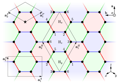
Figure 1: The honeycomb structure spans the crystallographic plane $\mathbf{a}\!=\![\overline{1},\overline{1},2]/\sqrt{6}$ and $\mathbf{b}\!=\![1,\overline{1},0]/\sqrt{2}$, perpendicular to $\mathbf{c}\!=\!\mathbf{a}\!\times\!\mathbf{b}\!=\![1,1,1]/\sqrt{3}$, written in cubic coordinates $xyz$. Red, green, and blue indicate NN X-, Y- and Z-bonds respectively, which are parallel to $[0\overline{1}1]$, $[10\overline{1}]$, and $[\overline{1}10]$ directions respectively. A primitive $(\mathbf{a}^{P}_{1},\mathbf{a}^{P}_{2})\!=\!\sqrt{2}([\overline{2},1,1],[1,\overline{2},1])$ unit cell is shown, with the two sublattice in fractional coordinates $(1/3,2/3)$, $(2/3,1/3)$. The crystallographic inversion center is shown by a star. The honeycomb hexagons can be partitioned into three disjoint groups H_x, H_y, H_z, shaded, respectively, by red, green, and blue, up to hexagon conventional unit cell translations $(\mathbf{a}^{H}_{1},\mathbf{a}^{H}_{2})\!=\!(2\mathbf{a}^{P}_{1}\!+\!\mathbf{a}^{P}_{2},\mathbf{a}^{P}_{1}\!+\!2\mathbf{a}^{P}_{2})$. The armchair unit cell $(\mathbf{a}^{A}_{1},\mathbf{a}^{A}_{2})\!=\!(\mathbf{a}^{P}_{1}\!-\!\mathbf{a}^{P}_{2},\mathbf{a}^{P}_{1}\!+\!\mathbf{a}^{P}_{2})$ is also shown.

The $K$-$\Gamma$ model on the honeycomb lattice reads

$$\begin{array}[]{c}\mathcal{H}=\mathcal{H}^{(\text{X})}+\mathcal{H}^{(\text{Y})}+\mathcal{H}^{(\text{Z})},\\ \mathcal{H}^{(\text{X})}=\displaystyle\sum\limits_{\langle ij\rangle\in\text{X}}\!\left[KS_{i}^{x}S_{j}^{x}+\Gamma\!\left(\!S_{i}^{y}S_{j}^{z}\!+\!S_{i}^{z}S_{j}^{y}\right)\right],\\ \mathcal{H}^{(\text{Y})}=\displaystyle\sum\limits_{\langle ij\rangle\in\text{Y}}\!\left[KS_{i}^{y}S_{j}^{y}+\Gamma\!\left(\!S_{i}^{z}S_{j}^{x}\!+\!S_{i}^{x}S_{j}^{z}\right)\right],\\ \mathcal{H}^{(\text{Z})}=\displaystyle\sum\limits_{\langle ij\rangle\in\text{Z}}\!\left[KS_{i}^{z}S_{j}^{z}+\Gamma\!\left(\!S_{i}^{x}S_{j}^{y}\!+\!S_{i}^{y}S_{j}^{x}\right)\right],\end{array}$$ (1)

where $\langle ij\rangle$ denote nearest neighbor lattice sites forming an X-, Y-, or Z-type of bond, shown, respectively, by red, green and blue in Fig. 1. This Figure also shows the conventional unit cells and their spanning vectors, as well as the crystallographic ‘$abc$’ and cubic ‘$xyz$’ frame.

The model has a $D_{3d}$ point group, consisting of threefold rotations $C_{3}$ around the out of plane $\mathbf{c}$-axis, twofold rotations $C_{2\text{X}(\text{Y}\text{Z})}$ around the X(YZ)-bond directions, inversion (through the center of any hexagon plaquette), as well as the mirror symmetries $m_{\text{X}(\text{Y}\text{Z})}=IC_{2\text{X}(\text{Y}\text{Z})}$ and improper rotations $S_{6}=IC_{3}$.

Besides the space group symmetries, the model has three global, site-dependent, symmetries $\mathcal{R}_{x}$, $\mathcal{R}_{y}$ and $\mathcal{R}_{z}$, corresponding to six-sublattice operations in the spin-space alone, that map the Hamiltonian to itself, see supplementing material of Ref. [28] and Ref. [9]. To see this one can define a six-sublatice conventional hexagon unit cell ($\mathbf{a}_{1}^{H}$, $\mathbf{a}_{2}^{H}$) that tiles the entire honeycomb. Based on these translations we can partition the set of all hexagons into three disjoint subsets H_x, H_y, H_z, shown as red, green, and blue subsets respectively in Fig. 1. Using the site labeling of Fig. 1, the $\mathcal{R}$ symmetries can be written as the following combinations of two-fold rotations $\mathsf{C}_{2x(yz)}$ (around cubic $x,\,y,\,z$ axes) in spin space:

$$\begin{array}[]{l}\mathcal{R}_{x}\!=\!\displaystyle\prod\limits_{i\in\{2,3\}}\!\mathsf{C}_{2x}(i)\!\prod\limits_{j\in\{1,6\}}\!\mathsf{C}_{2y}(j)\!\prod\limits_{k\in\{4,5\}}\!\mathsf{C}_{2z}(k),\\ \mathcal{R}_{y}\!=\!\displaystyle\prod\limits_{i\in\{5,6\}}\!\mathsf{C}_{2x}(i)\!\prod\limits_{j\in\{3,4\}}\!\mathsf{C}_{2y}(j)\!\prod\limits_{k\in\{1,2\}}\!\mathsf{C}_{2z}(k),\\ \mathcal{R}_{z}\!=\!\displaystyle\prod\limits_{i\in\{1,4\}}\!\mathsf{C}_{2x}(i)\!\prod\limits_{j\in\{2,5\}}\!\mathsf{C}_{2y}(j)\!\prod\limits_{k\in\{3,6\}}\!\mathsf{C}_{2z}(k)\,.\end{array}$$ (2)

For instance, the $\mathcal{R}_{z}$ transformation can be visualized as

(3)

Note that the operations $\mathcal{R}_{x}$, $\mathcal{R}_{y}$ and $\mathcal{R}_{z}$ can be thought of as products of the Kitaev’s plaquette operators [19] sitting on the H_x, H_y, or H_z subsets. The three $\mathcal{R}_{\alpha}$ operators, together with the identity, form the Klein four-group, i.e, $\mathcal{R}_{\alpha}\mathcal{R}_{\beta}\!=\!\mathcal{R}_{\gamma}$ and $\mathcal{R}_{\alpha}\!=\!\mathcal{R}_{\alpha}^{-1}$. Due to their site-dependent nature, these symmetries can mix the local character of any state in a nontrivial way. As we shall see, this leads to degeneraces between very different looking orders.

The $K$-$\Gamma$ model has a hidden SU(2) symmetry when $K\!=\!\Gamma$. The associated transformation is again a six-sublattice operation in spin space alone [48], which, for the H_z subset of the hexagons, can be written as [9]

$$\begin{array}[]{lclcrrr}\lx@intercol\hfil\small\mathcal{T}_{6z}~{}\text{transformation:}\hfil\lx@intercol\\ \widetilde{\mathbf{S}}_{1}=\mathbf{S}_{1}&\Rightarrow&\mathbf{S}_{1}&=(&\widetilde{S}_{1}^{x},&\widetilde{S}_{1}^{y},&\widetilde{S}_{1}^{z}),\\ \widetilde{\mathbf{S}}_{2}=\mathsf{C}_{2\text{Z}}\mathbf{S}_{2}&\Rightarrow&\mathbf{S}_{2}&=(&-\widetilde{S}_{2}^{y},&-\widetilde{S}_{2}^{x},&-\widetilde{S}_{2}^{z}),\\ \widetilde{\mathbf{S}}_{3}=\mathsf{C}_{3}^{-1}\mathbf{S}_{3}&\Rightarrow&\mathbf{S}_{3}&=(&\widetilde{S}_{3}^{y},&\widetilde{S}_{3}^{z},&\widetilde{S}_{3}^{x}),\\ \widetilde{\mathbf{S}}_{4}=\mathsf{C}_{3}\mathsf{C}_{2\text{Z}}\mathbf{S}_{4}&\Rightarrow&\mathbf{S}_{4}&=(&-\widetilde{S}_{4}^{x},&-\widetilde{S}_{4}^{z},&-\widetilde{S}_{4}^{y}),\\ \widetilde{\mathbf{S}}_{5}=\mathsf{C}_{3}\mathbf{S}_{5}&\Rightarrow&\mathbf{S}_{5}&=(&\widetilde{S}_{5}^{z},&\widetilde{S}_{5}^{x},&\widetilde{S}_{5}^{y}),\\ \widetilde{\mathbf{S}}_{6}=\mathsf{C}_{3}^{-1}\mathsf{C}_{2\text{Z}}\mathbf{S}_{6}&\Rightarrow&\mathbf{S}_{6}&=(&-\widetilde{S}_{6}^{z},&-\widetilde{S}_{6}^{y},&-\widetilde{S}_{6}^{x}).\\ \end{array}$$ (4)

where $(S_{i}^{x},S_{i}^{y},S_{i}^{z})$ are the components in the (global) cubic $xyz$ frame, and $(\widetilde{S}_{i}^{x},\widetilde{S}_{i}^{y},\widetilde{S}_{i}^{z})$ are the components in the rotated, site-dependent frame. The transformations $\mathcal{T}_{6x}$ and $\mathcal{T}_{6y}$ on the H_x and H_y subsets of hexagons are defined accordingly. To see the hidden SU(2) symmetry, we consider, e.g., the interactions on a Z-bond (1,2). Under $\mathcal{T}_{6z}$, we have

$$KS_{1}^{z}S_{2}^{z}+\Gamma(S_{1}^{x}S_{2}^{y}+S_{1}^{y}S_{2}^{x})\mapsto-K\widetilde{S}_{1}^{z}\widetilde{S}_{2}^{z}-\Gamma(\widetilde{S}_{1}^{x}\widetilde{S}_{2}^{x}+\widetilde{S}_{1}^{y}\widetilde{S}_{2}^{y}),$$ (5)

which, in turn, maps to $-K\ \widetilde{\bf S}_{1}\!\cdot\!\widetilde{\bf S}_{2}$ when $K\!=\!\Gamma$. The same holds for the other bonds. Thus, the point $\!K\!=\!\Gamma\!<\!0$ is a hidden SU(2) AFM point, and the point $\!K\!=\!\Gamma\!>\!0$ is a hidden SU(2) FM point.

Finally, we note that, in the classical model, there exists a duality transformation which flips the spins of the second sublattice of the honeycomb. Since this requires acting with time reversal on half of the sites, this transformation is only possible in the classical regime. In this regime, the duality effectively maps $(K,\Gamma)\!\to\!(-K,-\Gamma)$, so the classical phase diagram for a given set of couplings can be obtained from that of the opposite couplings. This leads to two, qualitatively different regions in the parameter space, the ones where $K$ and $\Gamma$ have the same sign, and the ones with opposite signs.

III Summary of known results about the Classical phase diagram of the $K$-$\Gamma$ model

Before we present our results, it is instructive to briefly review the main known features of the phase diagram of $K$-$\Gamma$ model. As usual, we parameterize the two couplings of the model in terms of an angle $\psi$, as

$$K=\cos\psi,\ \Gamma=\sin\psi\,,$$ (6)

and work in energy units of $\sqrt{K^{2}+\Gamma^{2}}=1$. In the regions $\psi\!\in\![0,\pi/2]$ and $\psi\!\in\![\pi,3\pi/2]$, where $K$ and $\Gamma$ have the same sign, we can use the following recipe to get the classical ground states [28, 36]: for every site $i$, write the components of the spin as $\mathbf{S}_{i}\!=\![x_{i},y_{i},z_{i}]$ with $x_{i}^{2}\!+\!y_{i}^{2}\!+\!z_{i}^{2}\!=\!S^{2}$, and then align its NN spins along $\zeta[x_{i},z_{i},y_{i}]$, $\zeta[z_{i},y_{i},x_{i}]$, or $\zeta[y_{i},x_{i},z_{i}]$, if the two sites share, respectively, an X-, Y-, or Z-bond, and $\zeta\!=\!-\operatorname{sgn}(K)=\!-\operatorname{sgn}(\Gamma)$. Schematically,

(7)

The energy contributions from the three bonds emanating from each site $i$ add up to $-(|K|+2|\Gamma|)(x_{i}^{2}\!+\!y_{i}^{2}\!+\!z_{i}^{2})\!=\!-(|K|+2|\Gamma|)S^{2}$. Since each bond is shared by two sites, the configurations that are generated by the above recipe saturate the energy lower bound $E_{\text{min}}/N\!=\!-(|K|/2+|\Gamma|)S^{2}$, and are therefore ground states.

Denoting by $[x_{o},y_{o},z_{o}]$ the spin of a starting, reference site, we can apply the above recipe to its first neighbours, and then to the second neighbours, and so on, until we cover the whole lattice. The resulting configurations take the form

(8)

with the following features, for general $[x_{o},y_{o},z_{o}]$:

i) There are six spin directions, $\mathbf{A}$ through $\mathbf{F}$, with spins pointing along the directions

$$\!\!\begin{array}[]{lll}{\bf A}\!=\![x_{o},y_{o},z_{o}],&{\bf B}\!=\![y_{o},z_{o},x_{o}],&{\bf C}\!=\![z_{o},x_{o},y_{o}],\\ {\bf D}\!=\!\zeta[y_{o},x_{o},z_{o}],&{\bf E}\!=\!\zeta[x_{o},z_{o},y_{o}],&{\bf F}\!=\!\zeta[z_{o},y_{o},x_{o}]\,.\end{array}$$ (9)

ii) The states form a two-parameter manifold, associated with the choice of $[x_{o},y_{o},z_{o}]$ of the reference site.

iii) The states break translational symmetry, with the underlying superlattice shown by dashed lines in Eq. (8) i.e., the Wigner-Seitz cell of the conventional hexagonal unit cell ($\mathbf{a}_{1}^{H}$, $\mathbf{a}_{2}^{H}$) from Fig. 1.

iv) Going from $\mathbf{A}\!\to\!\mathbf{B}\!\to\!\mathbf{C}$ is achieved by successive clockwise 120^∘ spin rotation around the $\mathbf{c}$-axis (even parity cyclic permutations of $[x_{o},y_{o},z_{o}]$), while for $\mathbf{D}\!\to\!\mathbf{E}\!\to\!\mathbf{F}$ the spin rotation is counter-clockwise (odd parity cyclic permutations of $[x_{o},y_{o},z_{o}]$). So, the classical ground states feature a period-3 modulation with two counter-rotating sublattices. This is one of the key ramifications of the interplay between $K$ and $\Gamma$, and here it arises simply from the requirement to saturate the energy contributions from both couplings along all bonds.

vi) In the local frames defined by the $\mathcal{T}_{6}$ transformation of Eq. (4), the above states map to the (much simpler) collinear Néel state (with moments along $\widetilde{\mathbf{S}}_{i}=\pm[x_{o},y_{o},z_{o}]$) for $\zeta=-1$, or the FM state (with moments along $\widetilde{\mathbf{S}}_{i}=[x_{o},y_{o},z_{o}]$) for $\zeta=1$. So, for negative $K$ and $\Gamma$, we end up with a ‘dual Néel’ phase, which includes the hidden SU(2) point $\psi\!=\!5\pi/4$, and, similarly, for positive $K$ and $\Gamma$, we get a ‘dual FM’ phase, which includes the hidden SU(2) point $\psi\!=\!\pi/4$.

It should be noted that at the isolated Kitaev points or the isolated $\Gamma$ points, there are infinitely more ground states, which can be generated by the two recipes described in Ref. [28] and [36]. The construction of (7) is essentially a combination of those two recipes, which works when the two couplings have the same sign [9].

When $K$ and $\Gamma$ have opposite signs, the two recipes cannot be combined due to frustration, and the phase diagram is more complex. Various classical energy minimization approaches, such as iterative simulated annealing [44], classical Monte Carlo simulations [49, 50], and machine learning approach [46, 51] have been employed to study the phase diagram in this region. These studies coherently show that a big part of the phase diagram is occupied by magnetic orders with large unit cells and/or truly incommensurate phases, but overall there is no consensus on the overall structure of the classical phase diagram in this region. This part of the phase diagram is the main focus of our study.

\begin{overpic}[width=433.62pt,percent]{Fig2.pdf}\put(0.0,61.0){(a)} \put(0.0,56.5){(b)} \put(0.0,34.5){(c)} \end{overpic}

Figure 2: (a) Phase diagram in the region $\psi\!/\!\pi\!\in\![0.5,1.0]$. (b) Minimum classical energy, $E_{\text{Min}}$ as a function of $\psi/\pi$ (black curve), as obtained by stitching together results from Monte Carlo runs and trial ansatz minimizations. Blue and red curves show the first and second derivatives of $E_{\text{Min}}$, respectively. The peaks in the second derivative (red curve) indicate phase transitions. Note multiple weak peaks in the IP, subleading by two order of magnitude from the strong transitions $6^{\prime}$ $\rightarrow$ 16. (c) Static structure factors (SSF) of the minimum energy state at representative $\psi$, one from each of the five regions. (SSHs decomposed in the cubic coordinates for the same values of the representative values $\psi$ are also shown Fig. 13.) The magnitudes of the SSF peaks are shown in the logarithmic scale from largest black dot to smallest gray dot, with the over all values normalized individually for every $\psi$ to the largest peak of that case.

IV Classical phase diagram for $\bm{K\!<\!0}$ and $\bm{\Gamma\!>\!0}$

\begin{overpic}[width=216.81pt,percent]{Fig3.pdf}\put(0.5,30.0){(c)} \put(0.5,63.5){(b)} \put(0.5,97.0){(a)} \put(43.8,30.0){(f)} \put(43.8,63.5){(e)} \put(43.8,97.0){(d)} \end{overpic}

Figure 3: The ansatz 18C₃ state (a-c) and $6^{\prime}$ state (d-f). For each of the ansatz we show: a color coded sketch of the ansatz (a) and (d), that corresponds to Eq. (13) and (15), the real space configuration of the spin state (b) at $\psi\!/\!\pi=0.55$ and (e) at $\psi\!/\!\pi=0.85$, and their $\mathbf{R}$ dual state (c) and (f). Magnetic unit cells are indicated by a faint gray area. The $\mathcal{R}$ symmetries reveal dual state, with the that 18C₃ state being degenerate with a different 18 site order, and the $6^{\prime}$ state degenerate with another different 18 site order.

IV.1 Computational methods

We performed classical Monte Carlo simulation of the $K$-$\Gamma$ model employing a combination of simulated annealing and parallel tempering approaches. In the simulated annealing we used an exponential cooling scheduler, performing $100-200$ cooling steps, with $10^{5}-10^{6}$ sweeps per step, cooling from $T=3$ down to $T=10^{-7}$ (all energies and temperatures are given in units of $\sqrt{K^{2}+\Gamma^{2}}$). In parallel tempering, we simulate $256$ replicas, with temperature logarithmically spread between $T=3$ and $T=10^{-5}$, and performing $10^{5}$ temperature updates for smaller clusters and up to $0.5\times 10^{6}$ for the largest clusters, with 100 sweeps between updates. One sweep consists of system-size number of Metropolis–Hastings trial updates. After Monte Carlo methods, we further refine the states by promoting

$$\mathcal{H}\rightarrow\widetilde{\mathcal{H}}=\mathcal{H}+\sum_{i}\lambda_{i}(\mathbf{S}_{i}\!\cdot\!\mathbf{S}_{i}-1),$$ (10)

using Lagrange multipliers $\lambda_{i}$, and minimizing the residual of the extrema equations $(\partial_{S_{i}^{\alpha}}\widetilde{\mathcal{H}},\partial_{\lambda_{i}}\widetilde{\mathcal{H}})=0$ with the aid of the non-linear optimization Ceres Library [52]. Minimization has also been performed by the torque updates, where demanding that the ground state be a stationary state, i.e., the time derivative as given by the Landau–Lifshitz–Gilbert equation [53] be set to zero $\mathrm{d}S^{\alpha}_{i}/\mathrm{d}t=-\varepsilon^{\alpha\beta\gamma}S^{\beta}_{i}(\partial\mathcal{H}/\partial S^{\gamma}_{i})=0$, imposes that every site by aligning with the local field

$$\mathbf{S}_{i}\rightarrow\mathbf{S}^{\prime}_{i}=-\mathbf{S}_{i}\times\mathbf{B}_{i}/\left\|\mathbf{S}_{i}\times\mathbf{B}_{i}\right\|,$$ (11)

where $B_{i}^{\alpha}=\partial\mathcal{H}/\partial S^{\gamma}_{i}$. The updates are performed repeatedly, until the convergence criteria $\mathrm{Max}\left[\left\|\mathbf{S}^{\prime}_{i}-\mathbf{S}_{i}\right\|\right]<10^{-15}$ is satified. We find that the Lagrange multiplier non-linear optimization and the torque update minimization have matching results.

IV.2 General aspects of the phase diagram

Combining all our numerical results, the resulting phase diagram for $K\!<0\!$ and $\Gamma\!>\!0$ is shown in Fig. 2 (a) and contains 5 extended regions, labeled as 18C₃, IP, $6^{\prime}$, 16 and zz. It is determined by the minimum classical energy $E_{\text{Min}}$ containing the combined information from all Monte Carlo runs, as well as ansatz minimization, across 10000 points in $\psi\!\in\![\pi/2,\pi]$, by always selecting the smallest energy state. In Fig. 2 (b) we show the evolution of the classical energy $E_{\text{Min}}$ (black curve), along with the first and second derivatives with respect to $\psi$ (blue and red curves, respectively), which signify the phase boundaries. For a selection of representative values of $\psi$, in Fig. 2(c) we show the static structure factors (SSF)

$$S(\mathbf{q})=\dfrac{1}{N}\sum\limits_{i,j}\mathrm{e}^{i\mathbf{q}\cdot(\mathbf{r}_{i}-\mathbf{r}_{j})}\mathbf{S}_{i}\!\cdot\!\mathbf{S}_{j}$$ (12)

up to the second Brillouin zone (BZ), for the corresponding ground states and their counterparts (called ‘$\mathcal{R}$ dual’ in the following) resulting from the symmetry operations $\mathcal{R}_{x(yz)}$ of Eq. (2). The decomposition of the SSF in various polarization channels is shown in App. C.2.

Among the 5 extended regions, the 18C₃, $6^{\prime}$, 16 and zz phases (whose structure will be discussed in more detail below) have been identified previously in the literature [54, 49, 55], and the special points $\psi\!=\!\pi/2$ and $\pi$ have infinite classical ground states [33, 56]. The wide intermediate region occupies almost 40% of the phase diagram and comprises a cascade of transitions between states with varying periodicity. Evidence for this is revealed by the series of peaks in the second derivative of the ground state energy, $\partial^{2}_{\psi}E_{\text{Min}}$ shown in Fig. 2 (b). Similar peaks in the second derivative mark the boundary of the IP region to the 18C₃ phase on the left and to the $6^{\prime}$ phase on the right, as well as the transitions between the $6^{\prime}$, 16 and zz phases. The peaks for the latter transitions are three orders of magnitude higher that those in the IP.

While other global aspects of the various states are discussed in App. C, in the following we analyze the main characteristics of each phase separately.

IV.3 The 18C₃ phase

Let us now examine the phase diagram more closely. In the region $\psi/\pi\!\in\!(0.5,0.6]$, we obtain the threefold-symmetric order with 18 spin sublattices called 18C₃ order in Ref. [54], 18^η order in Ref. [49] and triple-meron crystal in Ref. [55]. Its region of stability is much smaller compared to that reported in the literature [54, 49, 55]. Its magnetic unit cell is the $(3\mathbf{a}^{P}_{1},3\mathbf{a}^{P}_{2})$ cluster, which we denote as $P_{3\times 3}$ in the following. Figure 3 (a) shows the sublattice decomposition of this state, while Figs. 3 (b-c) show the actual spin directions of this state and its dual counterpart for the representative point $\psi=0.55\pi$. The Cartesian components of the 18 sublattices have the general form

$$\begin{array}[]{lll}\lx@intercol\hfil\mathbf{A}\!=\!-[1,1,1]/\sqrt{3}\,,~{}~{}~{}\overline{\mathbf{A}}\!=\![1,1,1]/\sqrt{3},\hfil\lx@intercol\\ \mathbf{B}_{1}\!=\![x,y,z],&\mathbf{B}_{2}\!=\![z,x,y],&\mathbf{B}_{3}\!=\![y,z,x],\\ \widetilde{\mathbf{B}}_{1}\!=\![y,x,z],&\widetilde{\mathbf{B}}_{2}\!=\![z,y,x],&\widetilde{\mathbf{B}}_{3}\!=\![x,z,y],\\ \mathbf{C}_{1}\!=\![x_{\mathrm{r}},x_{\mathrm{r}},z_{\mathrm{r}}],&\mathbf{C}_{2}\!=\![z_{\mathrm{r}},x_{\mathrm{r}},x_{\mathrm{r}}],&\mathbf{C}_{3}\!=\![x_{\mathrm{r}},z_{\mathrm{r}},x_{\mathrm{r}}],\\ \mathbf{D}_{1}\!=\![x_{\mathrm{g}},x_{\mathrm{g}},z_{\mathrm{g}}],&\mathbf{D}_{2}\!=\![z_{\mathrm{g}},x_{\mathrm{g}},x_{\mathrm{g}}],&\mathbf{D}_{3}\!=\![x_{\mathrm{g}},z_{\mathrm{g}},x_{\mathrm{g}}],\\ \mathbf{E}_{1}\!=\![x_{\mathrm{b}},x_{\mathrm{b}},z_{\mathrm{b}}],&\mathbf{E}_{2}\!=\![z_{\mathrm{b}},x_{\mathrm{b}},x_{\mathrm{b}}],&\mathbf{E}_{3}\!=\![x_{\mathrm{b}},z_{\mathrm{b}},x_{\mathrm{b}}].\\ \end{array}$$ (13)

and, apart from ${\mathbf{A}}$ and $\overline{\mathbf{A}}$, all other components vary with $\psi$. The sublattices ${\mathbf{A}}$ and $\overline{\mathbf{A}}$ reside at the center of the magnetic unit cell shown by the shaded hexagons. The remaining sublattices can be grouped into several flavors ($\mathbf{B}$ through $\mathbf{E}$), and are depicted by different colors in Fig. 3 (a). Within each group, there are three sites that are $\mathsf{C}_{3}$ related, indicated by subscripts 1,2,3, and in this sense the sites swirl around the $\mathbf{A}$ center, see Fig. 3 (b). The sites of $\mathbf{B}$ and $\widetilde{\mathbf{B}}$ groups have three non-zero spin components and are related to each other by $\mathsf{C}_{2}$ rotations, i.e., $\widetilde{\mathbf{B}}_{1}\!=\!-\mathsf{C}_{2\text{Z}}\mathbf{B}_{1}$, so we denote them by the similar letters. The sites on both magnetic $\mathbf{B}$ and $\widetilde{\mathbf{B}}$ groups, as well as the ${\mathbf{A}}$ and $\overline{\mathbf{A}}$ groups, reside on the same sublattice of the honeycomb lattice. The other sublattice of the honeycomb lattice hosts spins belonging to $\mathbf{C}$, $\mathbf{D}$, and $\mathbf{E}$ groups [depicted by red, green, blue colors in Fig. 3(a)]. These sites have $[x,x,z]$ character, i.e., they live on the $\mathbf{ac}$ plain. From the ansatz structure, we clearly see that honeycomb sublattice symmetry is broken in the 18C₃ state. We also note that 18C3 breaks the inversion symmetry. The inversion symmetry related state of 18C3 state with the center on the A sublattice (dubbed 18C${}_{3}^{A}$ in the following) will have its center on the B sublattice (dubbed 18C${}_{3}^{B}$).

The dual counterpart of the 18C₃ state, denoted by $\mathcal{R}(\text{18C${}_{3}$})$, also involves 18 sites, however, its internal structure is different and breaks the $\mathsf{C}_{3}$ symmetry, see Fig. 3 (c). This is due to the nontrivial, site-dependent nature of the $\mathcal{R}$ transformations.

The SSFs of the 18C₃ state and its dual are shown in the first column of Fig. 2 (c). The $C_{3}$ character of the 18C₃ state is characterized by a 3Q-pattern inside both the first and second BZ, where peaks reside at the points $\pm 2{\bf M}/3$ and $\pm 4{\bf M}/3$, along with subdominant peaks at the boundary of the second BZ, and with all $C_{3}$ related momenta having the same weight (as expected by symmetry). By contrast, the dual $\mathcal{R}(\text{18C${}_{3}$})$ loses this behaviour. Its SSF is dominated by the $2{\bf M}/3$ momentum points, with subdominant contribution from the $\mathbf{K}$ points of the BZ and a residual $\mathbf{q=0}$ contribution. Note that if we were to disregard the influence of the residual points, the system would exhibit a state characterized by only 6 magnetic sublattices, as in the $6^{\prime}$ state, which will be discussed in Sec. IV.4. However, due to the presence of these residual points, we observe a truly intricate 18-magnetic-sublattice order within this region of the phase diagram, both in the original and the dual spin space. As we discuss in Sec. IV.8 below, due to this complex spin structure, the 18$C_{3}$ state possesses a non-zero total scalar chirality, the largest among the various states of the phase diagram.

\begin{overpic}[width=216.81pt,percent]{Fig4.pdf}\put(0.5,97.5){(a)} \put(0.5,39.0){(b)} \end{overpic}

Figure 4: (a) Common-origin plot of the spin directions in the 18C₃ state at $\psi\!=\!0.55\pi$ (arrows) and in its ‘parent’ state at $\psi\!\to\!(\pi/2)^{+}$, given by Eq. (14) $\psi\!\to\!(\pi/2)^{+}$ (thin lines). b) Comparison between the corresponding SSFs of the two states.

The ‘parent 18C₃’ state. We will now show that the 18C₃ state can be thought of as a slightly distorted version of its limiting structure at $\psi\!\to\!(\pi/2)^{+}$. In this limit, the 18$C_{3}$ state becomes a member of the infinitely degenerate ground state manifold of the pure $\Gamma$ point [28]. Indeed, in this limit, the Cartesian components of Eq. (13) tend to

$$\begin{array}[]{c}\mathbf{A}=-\overline{\mathbf{A}}=\mathbf{E}_{1}=\mathbf{E}_{2}=\mathbf{E}_{3}=\!=\!-[1,1,1]/\sqrt{3},\\ \mathbf{B}_{1}=\widetilde{\mathbf{B}}_{1}=\mathbf{C}_{1}=-\mathbf{D}_{1}=[1,1,-1]/\sqrt{3},\\ \mathbf{B}_{2}=\widetilde{\mathbf{B}}_{2}=\mathbf{C}_{2}=-\mathbf{D}_{2}=[-1,1,1]/\sqrt{3},\\ \mathbf{B}_{3}=\widetilde{\mathbf{B}}_{3}=\mathbf{C}_{3}=-\mathbf{D}_{3}=[1,-1,1]/\sqrt{3}.\end{array}$$ (14)

These directions satisfy the general recipe discussed in Ref. [28] and the state is therefore one of the ground states. Now, as shown in Fig. 4 (a), the 18C₃ state at a representative point inside the phase ($\psi\!=\!0.55\pi$) is quite similar to that of Eq. (14). This is further reflected in the almost identical SSFs shown in Fig. 4 (b). Therefore, the characteristic 3Q SSF profile of the 18C₃ state originates in the special, four-sublattice structure of the ‘parent 18C₃’ state, with spins pointing along the different [111] axes. The weak deviations of the spins away from these four primary directions of the parent state, which are caused by a negative $K$, amount to weak signals at ${\bf q}\!=\!0$ (evidencing a small nonzero magnetization) and the two corners of the 1st BZ (${\bf K}$-points).

IV.4 The $\mathbf{6^{\prime}}$ phase

The $6^{\prime}$ state is stable on the right side of the IP phase, in the region $\psi/\pi\!\in\![0.793,0.909]$. These boundaries align with those reported in the literature [49, 55], although they appear slightly shifted on the left side. The magnetic unit cell comprises 6 sublattices with only 3 different spin directions, all in the same plane. There are three versions of the $6^{\prime}$ state, related to each other by threefold rotations. Figure 3 (d) shows the sublattice decomposition of one of them, with spins living on the $\mathbf{ac}$ plane, and sublattices

$$\begin{array}[]{lll}\mathbf{A}\!=\![x_{\mathrm{r}},x_{\mathrm{r}},z_{\mathrm{r}}],&\mathbf{B}\!=\![x_{\mathrm{g}},x_{\mathrm{g}},z_{\mathrm{g}}],&\mathbf{C}\!=\![x_{\mathrm{b}},x_{\mathrm{b}},z_{\mathrm{b}}].\end{array}$$ (15)

The spatial profile of these sublattices shows a counter-rotating modulation, $\mathbf{ABC}\cdots$ vs $\mathbf{ACB}\cdots$, of the two honeycomb sublattices, similar to the so-called ‘$K$-state’ discussed in the 3D material $\beta$-Li₂IrO₃ [57].

The actual magnetization profiles of the $6^{\prime}$ state and its dual are shown in Figs. 3 (e-f) for the representative point $\psi\!=\!0.85\pi$. The corresponding SSFs are shown in the third column of Fig. 2 (c). The magnetic unit cell of the dual state $\mathcal{R}(6^{\prime})$ has 18 sites, three times larger than that of the $6^{\prime}$ state. The SSF of the $6^{\prime}$ state is dominated by four peaks at $\pm 2{\bf M}/3$ and $\pm 4{\bf M}/3$, and has residual contributions at the boundary of the second BZ and at $\mathbf{q=0}$. The latter shows that this state features a nonzero total moment. The SSF of the dual state is similar to the SSF of the $\mathcal{R}(\text{18C}_{3})$ state if we ignore subdominant peaks, suggesting a deeper connection between the two phases. Indeed, we have found that the characteristic ABC-structure in the $6^{\prime}$ configuration, with spins in the ${\bf ab}$-plane, can be reproduced (modulo a spin-length normalization for the vectors ${\bf A}$, ${\bf B}$ and ${\bf C}$) by the following linear combination of different replica of the 18C₃ state:

$$6^{\prime}\!\propto\!\Big{(}1+\mathcal{T}_{{\bf a}^{A}_{2}}+\mathcal{T}_{2{\bf a}^{A}_{2}}\Big{)}\cdot\Big{(}\text{18C}_{3}^{A}\!+\!\text{18C}_{3}^{B}\Big{)}\,,$$ (16)

where the translation operator $\mathcal{T}_{\bf a}$ moves the spins by lattice vector distances $\mathcal{T}_{\bf a}\cdot{\bf S}_{A(B),{\bf R}}\!=\!{\bf S}_{A(B),{\bf R}+{\bf a}}$, and $\mathbf{a}_{2}^{A}\!=\!\mathbf{a}_{1}^{P}\!+\!\mathbf{a}_{2}^{P}$ one of the armchair lattice vectors, see Fig. 1. This construction, elaborated in App. B, shows that contrary to the 18C3 state, 6’ state restores the inversion symmetry.

IV.5 The 16 phase

The phase labeled as ‘16’ in Fig. 2 (a) is stable in the narrow region $\psi/\pi\in[0.909,0.926]$ and has a magnetic unit cell with 16 sites, which in turn belong to 8 different spin directions. As in the $6^{\prime}$ state, the spins are again coplanar and there are three versions of the 16 order, related to each other by threefold rotations. Figure 5 (a) shows the sublattice decomposition of one of them, with spins living on the ${\bf ac}$ plane, and sublattices given by

$$\begin{array}[]{ll}\mathbf{A}\!=\![x_{\mathrm{r}},x_{\mathrm{r}},z_{\mathrm{r}}],&\overline{\mathbf{A}}\!=\!-{\bf A},\\ \mathbf{B}\!=\![x_{\mathrm{g}},x_{\mathrm{g}},z_{\mathrm{g}}],&\overline{\mathbf{B}}\!=\!-{\bf B},\\ \mathbf{C}\!=\![x_{\mathrm{b}},x_{\mathrm{b}},z_{\mathrm{b}}],&\overline{\mathbf{C}}\!=\!-{\bf C},\\ \mathbf{D}\!=\![x_{\mathrm{y}},x_{\mathrm{y}},z_{\mathrm{y}}],&\overline{\mathbf{D}}\!=\!-{\bf D},\end{array}$$ (17)

The magnetization profiles of this state and its dual counterpart $\mathcal{R}(16)$ (whose magnetic unit cell contains 48 sites) are shown in Figs. 5 (b-c), for the representative point $\psi\!=\!0.917\pi$. Their corresponding SSFs are shown in the fourth column of Fig. 2 (c). The SSF of the 16 state shows dominant peaks at $\pm 3{\bf M}/4$ and $\pm 5{\bf M}/4$, and a bit smaller peaks at $\pm{\bf M}/4$ and $\pm 7{\bf M}/4$. Comparing to the neighboring phases, it appears as if the $6^{\prime}$ state with dominant peaks at $\pm 2{\bf M}/3$ is attempting to move towards the zz state with peaks at the ${\bf M}$ points, however it happens through the intermediate small window of the 16 state with dominant $\pm 3{\bf M}/4$ peaks [with visual representation in Fig.2 (c)].

IV.6 The zz phase

The zigzag (zz) order is stable for $\psi/\pi\!\in\![0.926,1)$. The appearance of this order may be attributed to the nearby hidden symmetry point $\mathcal{T}_{1}\mathcal{T}_{4}$ in the enlarged $J$-$K$-$\Gamma$-$\Gamma^{\prime}$ model [48], and has been seen to stabilize a sizeable zz region even for very small $\Gamma^{\prime}\!<\!0$ interactions compared to the $K$ and $\Gamma$ parameters [25].

The magnetic unit cell comprises 4 sites which belong to two different spin directions, aligned opposite to each other (i.e., the state is collinear). As in the phases $6^{\prime}$ and 16, there are three different versions of the zz phase, related to each other by threefold rotations. Figure 5 (d) shows one of them, with with spins living on the $\mathbf{ac}$ plane and sublattices given by

$$\mathbf{A}\!=\![x,x,z]\,,~{}~{}\overline{\mathbf{A}}\!=\!-{\bf A}$$ (18)

The magnetization profiles of the zz state and its dual counterpart $\mathcal{R}(\text{zz})$ (whose magnetic unit cell contains 12 sites) are shown in Figs. 5 (e-f) for the representative point $\psi\!=\!0.95\pi$. The corresponding SSFs are shown in the last column of Fig. 2 (c), with the SSF of the zz state having the standard Bragg peaks at one of the three ${\bf M}$ points of the BZ.

Finally, we note that in the limit of $\psi\!\to\!\pi^{-}$, the zz state becomes a member of the infinitely degenerate ground state manifold of the pure Kitaev point [33, 34, 36]. Indeed, in this limit, the Cartesian components of Eq. (18) tend to

$$\overline{\mathbf{A}}\!=\!-{\bf A}=[1,1,0]/\sqrt{2}.$$ (19)

These directions satisfy the general recipe discussed in Ref. [36] and the state is therefore one of the ground states.

\begin{overpic}[width=216.81pt,percent]{Fig5.pdf}\put(0.5,30.0){(c)} \put(0.5,63.5){(b)} \put(0.5,97.0){(a)} \put(58.5,30.0){(f)} \put(58.5,63.5){(e)} \put(58.5,97.0){(d)} \end{overpic}

Figure 5: The ansatz 16 state (a-c) and zz state (d-f). For each of the ansatz we show: a color coded sketch of the ansatz (a) and (d), that corresponds to Eq. (17) and (18), the real space configuration of the spin state (b) and (e), and the $\mathbf{R}$ dual state (c) and (f). Magnetic unit cells are indicated by a faint gray area. The $\mathcal{R}$ symmetries reveal dual state, with the that 16 state being a 48 site order, and the zz state degenerate with a 12 site order.

\begin{overpic}[width=433.62pt,percent]{Fig6.pdf}\put(2.0,33.5){(a)} \put(35.0,33.5){(b)} \put(67.8,33.5){(c)} \put(2.0,16.5){(d)} \put(35.0,16.5){(e)} \put(67.8,16.5){(f)} \end{overpic}

Figure 6: Energy per site plots as a function of armchair cluster length $n$, as found from Monte Carlo simulations. The simulated clusters are $A_{3\times n}$ clusters, as illustrated in (a). Total energies obtained by the Monte Carlo simulations for $\psi/\pi=$ $0.65$ (b), $0.7$ (c), $0.725$ (d), $0.75$ (e), and $0.775$ (f) show deviations from the energy of the 18C₃ and $6^{\prime}$ states indicated by horizontal gray lines. Note that in panel (f) the energy of the 18C₃ has become higher that the $6^{\prime}$. We see a universal behaviour: the results partition into three curves $3|n$ (red), $3|(n-1)$ (green), and $3|(n-2)$ (blue). The oscillatory behaviour of the curves as a function of $n$ is interpreted as a signature of incommensuration.

IV.7 The intermediate phase

IV.7.1 Energetics of finite-size clusters

The IP occupies a considerable region of the phase diagram $\psi/\pi\!\in\![0.6,0.793]$. Previous studies  [44, 58, 49, 46, 59, 50] suggested that this region consists of phases with large magnetic unit cells or long-wavelength, incommensurate modulations. While such orders with large (or infinite) unit cells are challenging to study in finite-size simulations, the associated multi-peaked SSFs offer distinctive fingerprints for their experimental detection. This is why here we perform a detailed analysis of this phase by employing numerical simulations on the most suitable elongated armchair clusters.

The armchair building block is a conventional rectangle unit cell, spanned by $(\mathbf{a}_{1}^{A},\mathbf{a}_{2}^{A})$ lattice vectors, parallel to $\mathbf{a}$ and $\mathbf{b}$ directions, see Fig. 1. The elongated clusters that host the IP state have a structure of $(3\mathbf{a}_{1}^{A},n\mathbf{a}_{2}^{A})\!\equiv\!A_{3\times n}$, see Fig. 6 (a). By construction the zz state fits on any armchair. The 16-site state needs at least the $A_{4\times 1}$ cluster and is not compatible with any $A_{3\times n}$ clusters. The $6^{\prime}$ state commensurates with the $A_{3\times 1}$ cluster, exactly two copies of it. The 18C₃ state lives on the $P_{3\times 3}$ cluster, which commensurates with $A_{3\times n}$ clusters only if $n$ is divisible by 3, or in math notation $3|n$. The $\mathcal{R}$ operations need at least the hexagonal $(\mathbf{a}_{1}^{H},\mathbf{a}_{2}^{H})$ unit cell, which commensurates with the primitive $P_{3\times 3}$, and consequently commensurates with $A_{3\times n}$ when $3|n$. Further details on commensurability of the $P_{m\times m}$ clusters with $A_{3\times n}$ clusters can be found in App. A.

We performed Monte Carlo simulations on the $A_{3\times n}$ clusters with $1\!\leq\!n\!\leq\!60$ and for $\psi/\pi\!=$0.65, 0.7, 0.725, 0.75, 0.775. Results for the energy per site as a function of $n$ are shown in Fig. 6 (b-f). For comparison, we also indicate, by labelled horizontal gray lines, the (variational) energies per site of the 18C₃ and $6^{\prime}$ states for each given parameter point. Some general trends, that are particularly well seen in the insets of Fig. 6 (b-f), emerge from our simulations. The energy curves naturally partition into three families: $3|n$ (red curve), $3|(n-1)$ (green curve), and $3|(n-2)$ (blue curve). The $3|n$ family fits the 18C₃ state and stabilizes it for a large window of $n$, until eventually the energy gets lower than that of 18C₃, suggesting states with even larger unit cells, or, even incommensurate states. Similarly, the energies of the $3|(n-1)$ and $3|(n-2)$ families, after a short window of $n$, get below the energy of the $6^{\prime}$ state and eventually below that of the 18C₃ for $n$ sightly larger than 6. The first curve to drop, for any $\psi$, is $3|(n-1)$, then $3|(n-2)$, and finally $3|n$. For each curve, the energy appears to oscillate. Moreover, the minimum switches between families. These results are suggestive of an incommensurate state being accommodated on finite-size clusters.

\begin{overpic}[width=216.81pt,percent]{Fig7.pdf}\put(0.5,98.5){(a)} \put(20.0,98.5){(b)} \put(20.0,78.0){(c)} \put(20.0,60.0){(d)} \end{overpic}

Figure 7: (a) The IP state, for $\psi/\pi\!=\!0.7$ hosted on the $A_{3\times 39}$ cluster ($3|n$ familiarly). (b) Common origin plot of spins, resolved on the $A_{3\times 3}$ subcluster ($13A_{3\times 3}=A_{3\times 39}$), where sublattice A(B) colored in red(blue). Gray arrows indicating the average direction of the “near-cone” formed by the precessing spins [note that these gray arrows follow the directions of the $\mathcal{R}(6^{\prime})$ state, compare to Fig. 3 (f)]. The red ($A$ sublattice) and blue ($B$ sublattice) near-cones counter rotate to eachother, shown more clearly in (c) for two example common origin points. (d) Zoom in windows of the elongated state, highlighting the switch of 18C₃ like local windows, from $A$ (red circle) to $B$ (blue circle) sublattice, approximately half way through the cluster.

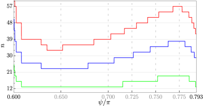
Figure 8: Tracking the cluster’s length $n$ of the minimum energy state within the three families: $3|n$ (red), $3|(n-1)$ (green), and $3|(n-2)$ (blue). Dashed gray lines indicate the $\psi$ points for which $A_{3\times n}$ clusters were simulated in Monte Carlo for $n$ up to 60. The rest of the points were calculated by Lagrange multiplier minimization using Monte Carlo result as an input, also supplemented with torque updates.

IV.7.2 Static structure factors

We computed the SSFs for several $\psi$ points in the intermediate phase, and they appear to be similar in all cases. For all points, magnetic orders obtained by the Monte Carlo simulations on the finite $A_{3\times n}$ clusters appear to utilize the entire cluster length with no sub-periods. To illustrate their structure, we plot in the second column of Fig. 2 (c) the SSF of the IP and its $\mathcal{R}$-dual (diagonal components of SSH in cubic coordinates are shown Fig. 13), as obtained for $\psi/\pi\!=\!0.7$ on the cluster with $n\!=\!39$ belonging to the $3|n$ family. The SSFs exhibit a sequence of well-defined Bragg peaks, accompanied by additional trailing points in the vicinity of these peaks. Notably, the positions and relative intensities of the sharp Bragg peaks resemble closely those of the neighbouring 18C₃ and $\mathcal{R}(6^{\prime})$ states, while all trailing points exhibit vertical displacement. These observations indicate a one-dimensional incommensurate modulation (here in the vertical direction) of the neighboring commensurate states.

IV.7.3 Local 18C₃ character

The corresponding magnetic state needs a large $3|n$ unit cell, so the real space visualization is rather difficult. Figure 7 (a) shows a zoomed out overview of the intermediate state for $\psi/\pi\!=\!0.7$, along with some zoomed in windows in panel (c). We observe a distinctive modulation of the magnetic order which can be best described by the switching between windows of local 18C₃-like character. Going sliver by sliver, at the bottom of the cluster we have a fragment of the 18C₃ state centered on the $A$ sublattice of the honeycomb lattice (referred to as 18$C_{3}^{A}$), then by moving vertically up along the cluster, all sublattices of 18C₃ state slowly undergo a gradual precession such that at about the middle of the cluster we see that the center of the 18C₃ switches to the honeycomb $B$ sublattice (referred to as 18$C_{3}^{B}$). These two regions are related by inversion symmetry i.e., 18$C_{3}^{B}$=$I($18$C_{3}^{A})$. This multi-sublattice magnetic order mimics the intermediate state and lowers the energy of the 18C₃ like centers via restoring the sublattice and inversion symmetry of the honeycomb lattice.

The switching of sublattices in the 18C₃-like centers is achieved through a non-trivial precession of the spins. To simplify the representation, we can collapse all the sites of the $A_{3\times 39}$ lattice down to a single $A_{3\times 3}$ window. Then each site serves as a common origin for plotting the spins. Those corresponding to the centers of the 18C₃ order shown in Fig. 7 (b) are depicted in Fig. 7 (c), with spins colored in red for the $A$ sublattice and blue for the $B$ sublattice. The spin configurations almost form cones but exhibit some deviation, and we shall refer to them as ‘near-cones’.

Let us first focus on the centers within the cluster that underwent a mid-cluster switch. Specifically, one center originated from the $A$ sublattice, while the other originated from the $B$ sublattice, in Fig. 7 (a) marked with red and blue circles, respectively. Interestingly, the near-cone associated with the $A$ sublattice and the one linked to the $B$ sublattice align perfectly in their orientations. However, a noteworthy observation is that these two near-cones exhibit counter-rotational precession relative to each other.

To gain further insight, we can calculate the average directions of the near-cones, which reveal the axis of precession. These average directions are indicated by the gray arrows in Fig. 7 (b). Upon closer examination, it becomes evident that this counter-rotational behavior is not limited to a specific region; instead, it persists throughout the system. Specifically, the near-cones associated with the $A$ sublattice exhibit a counter-clockwise traversal around their respective axes of precession, while those related to the $B$ sublattice undergo clockwise precession. Notably, the directions of precession within the system aligns with the directions of the spins observed in the $\mathcal{R}(6^{\prime})$ state. This observation implies that the dominant peaks in the SSF of the intermediate state stem from the magnetic structure described by the averaged directions of the spins, and the trailing points that extend away from these dominant peaks are due to the gradual precession of spins occurring on the near-cones.

Next, using the cluster length as an indication of the incommensurate repetition period and in order to examine the dependence of optimal cluster length on the model parameters, we use the Monte Carlo numerical states as the input for a more refined Lagrange multiplier minimization, in combination with torque updates. Our results are summarized in Fig. 8 where we track the energy minimum in every family and plot the optimal value of $n$ as a function of $\psi$. All three families in Fig. 8 (b) show a similar behaviour, indicative that all families are attempting to fit the same type of state as the ground state. Within each family, the cluster length $n$ for which the energy is minimized generally increases as $\psi$ increases.

Along with the smooth behaviour of cluster length in the majority of the IP, Fig. 8 (b) shows an increase in the optimal cluster’s size towards the left boundary to the 18C₃ state and a decrease towards the right boundary to the $6^{\prime}$ state. The sharp increase in cluster length as we approach the left boundary of the IP can be attributed to the 18C${}_{3}^{A}$ centres pushing away from the 18C${}_{3}^{B}$ centers in order to leave a single clean 18C₃ state. The transition between the 18C₃ and the IP can therefore be thought of as a continuous commensurate-incommensurate (C-I) transition, whereby the spin structure ‘rotates’ between different ‘domains’ (here 18C${}_{3}^{A}$ and 18C${}_{3}^{B}$) of a parent commensurate state (here the 18C₃ state), with the distance between the domains going to infinity at the transition [60, 61, 62, 63].

By contrast, the decrease of the cluster length $n$ at around $\psi/\pi\!=\!0.793$ suggests that the transition to the $6^{\prime}$ state is not a continuous C-I transition. In particular, the deeper connection between the $6^{\prime}$ and the 18C₃ states, as follows from Eq. (16), suggests that the sharp decrease of cluster length towards the $6^{\prime}$ boundary can be interpreted as merging of several 18$C_{3}$ windows to form the $6^{\prime}$ state.

IV.8 Evolution of scalar spin chirality profiles

\begin{overpic}[width=216.81pt,percent]{Fig9.pdf}\put(0.5,98.5){(a)} \put(0.5,71.0){(b)} \put(0.5,33.5){(c)} \end{overpic}

Figure 9: (a) Definition of chiralities $\chi^{(1)/(2)}_{A/B,\mathbf{R}}$ for sublattice $A$ (red) and $B$ (blue).(b) Plot of $\left\langle\chi\right\rangle$ for the original (solid lines) and $\mathcal{R}$ dual (doted lines) states, resolved on sublattices (red and blue) as well as the total (black). Dashed gray lines indicate the $\psi$ points for which $A_{3\times n}$ clusters where simulated in Monte Carlo, while other points in the IP are evaluated from Lagrange multiplier minimization. (c) Coarse-grained chirality $\left\langle\chi_{A(B)}\right\rangle_{m}$ with $0\!\leq\!m\!\leq\!n$. Each $\psi/\pi\!=\!0.65,0.7,0.725,0.75,0.775$ realizes the ground state on a cluster of different length,$n_{\psi}=33,39,45,51,57$ respectively, and the coarse-grained chirality is plotted as a function of the $\text{normalized}(m)=m/n_{\psi}$.

The visual representation of the intermediate state in Fig. 7 provides some hints that the nature of the IP can be understood as an incommensuration between 18$C_{3}^{A(B)}$ like centres. Aiming to quantify this behaviour, in this section we will discuss how inequivalence of the scalar chiralites for A and B triangular sublattices can be used to describe this incommensuration.

Scalar spin chirality is defined for each triangular plaquette formed by second-neighbour sites $i$, $j$ and $k$ as $\mathbf{S}_{i}\!\cdot\left(\mathbf{S}_{j}\!\times\!\mathbf{S}_{k}\right)$. If the moments on the plaquette are non-coplanar, the resulting scalar spin chirality is non-zero, $\langle\mathbf{S}_{i}\!\cdot\left(\mathbf{S}_{j}\!\times\!\mathbf{S}_{k}\right)\rangle\neq 0$ and breaks the time-reversal and the inversion symmetries. On the honeycomb lattice, with two sublattices $A$ and $B$ in the primitive unit cell located at position $\mathbf{R}$, four chiralities can be defined:

$$\begin{array}[]{l}\chi^{(1)}_{A,\mathbf{R}}\!\equiv\!\mathbf{S}_{A,\mathbf{R}}\!\cdot\!\left(\mathbf{S}_{A,\mathbf{R}+\mathbf{a}^{P}_{1}}\!\times\!\mathbf{S}_{A,\mathbf{R}+\mathbf{a}^{P}_{1}+\mathbf{a}^{P}_{2}}\right),\\ \chi^{(2)}_{A,\mathbf{R}}\!\equiv\!\mathbf{S}_{A,\mathbf{R}}\!\cdot\!\left(\mathbf{S}_{A,\mathbf{R}+\mathbf{a}^{P}_{1}+\mathbf{a}^{P}_{2}}\!\times\!\mathbf{S}_{A,\mathbf{R}+\mathbf{a}^{P}_{2}}\right),\\ \chi^{(1)}_{B,\mathbf{R}}\!\equiv\!\mathbf{S}_{B,\mathbf{R}}\!\cdot\!\left(\mathbf{S}_{B,\mathbf{R}+\mathbf{a}^{P}_{1}+\mathbf{a}^{P}_{2}}\!\times\!\mathbf{S}_{B,\mathbf{R}+\mathbf{a}^{P}_{2}}\right),\\ \chi^{(2)}_{B,\mathbf{R}}\!\equiv\!\mathbf{S}_{B,\mathbf{R}}\!\cdot\!\left(\mathbf{S}_{B,\mathbf{R}+\mathbf{a}^{P}_{1}}\!\times\!\mathbf{S}_{B,\mathbf{R}+\mathbf{a}^{P}_{1}+\mathbf{a}^{P}_{2}}\right),\end{array}$$ (20)

where superscript $(1)$ indicates triangles of $A(B)$ sublattice sites centred over an empty hexagon, and superscript $(2)$ triangles of $A(B)$ sublattice sites centred over a $B(A)$ sublattice site. The site ordering is chosen such that the sites are traversed anti-clockwise. In Fig. 9 (a) we show these quantities as red triangles for sublattice $A$, and blue triangles for sublattice $B$. Together, $\chi^{(1)}_{A(B),\mathbf{R}}$ and $\chi^{(2)}_{A(B),\mathbf{R}}$ tessellate the entire sublattice $A(B)$. The average chirality on each sublattice is

$$\left\langle\chi_{A(B)}\right\rangle\equiv\dfrac{1}{2N_{c}}\displaystyle\sum\limits_{\mathbf{R}}\left[\chi^{(1)}_{A(B),\mathbf{R}}+\chi^{(2)}_{A(B),\mathbf{R}}\right],$$ (21)

with $N_{c}$ the number of unit cells, and the factor of $\frac{1}{2}$ to normalize the average to unity, since $\chi^{(1)}$ and $\chi^{(2)}$ each have a maximum value of 1. We further define the coarse-grained chirality $\left\langle\chi_{A(B)}\right\rangle_{m}$ as the partial averaging of the scalar chirality over a window of $A_{3\times 3}$ centered at vertical location $m$,

$$\left\langle\chi_{A(B)}\right\rangle_{m}\!=\!\dfrac{1}{36}\displaystyle\sum\limits_{\mathbf{R}\in A_{3\times 3}}\left[\chi^{(1)}_{A(B),\mathbf{R}+m\mathbf{a}_{2}^{A}}\!+\!\chi^{(2)}_{A(B),\mathbf{R}+m\mathbf{a}_{2}^{A}}\right].$$ (22)

Similarly, we can define the coarse-grained chirality $\left\langle\chi_{A(B)}\right\rangle_{m}$ for a $A_{3\times n}$ cluster with $0\!\leq\!m\!\leq\!n-1$ running vertically throughout the entire cluster. We can compute, alternatively to Eq. (21, the average chirality of the entire cluster as

$$\left\langle\chi_{A(B)}\right\rangle=\dfrac{1}{n}\displaystyle\sum\limits_{m=0}^{n-1}\left\langle\chi_{A(B)}\right\rangle_{m}.$$ (23)

In Fig. 9 (b) we show the average chirality $\langle\chi_{A(B)}\rangle$ by a red(blue) solid curve for the original state and dotted lines for the $\mathcal{R}$ dual states. In the 18C₃ state, due to the sublattice imbalance indicated earlier, we see that the average chirality is also imbalanced with $\left\langle\chi_{A}\right\rangle\neq\pm\left\langle\chi_{B}\right\rangle$, however, all other states including the IP show a sublattice egalitarian behaviour of $\left\langle\chi_{A}\right\rangle=\left\langle\chi_{B}\right\rangle$. The chirality for states $6^{\prime}$, 16, and zz are all zero, and can be attributed to the surviving $m_{\text{Z}}$ mirror symmetry in all three states. A jump is seen going from the 18C₃ to the IP, however, going from the IP to the dual $\mathcal{R}(6^{\prime})$ 18-sublattice state looks continuous. This is consistent with the picture of $\mathcal{R}(6^{\prime})$ state being a commensurate limit of the IP.

For the minimum energy states of the $3|n$ family obtained for a set of points $\psi/\pi\!=$0.65, 0.7, 0.725, 0.75, 0.775, we examine the coarse-grained chirality $\left\langle\chi_{A(B)}\right\rangle_{m}$ while traversing the cluster vertically with $m$. Since for every $\psi$ the minima is on a different cluster length $n_{\psi}$, we normalize the length and plot $\left\langle\chi_{A(B)}\right\rangle_{m}$ as a function of normalized $(m)$=$m/n_{\psi}$, with $0\!\leq\!m\!\leq\!n_{\psi}$. In Fig. 9 (c) we see the coarse-grained chirality for the IP, plotted against $m$. Running through the cluster, we see that $\left\langle\chi_{A}\right\rangle_{m}\!=\!-\left\langle\chi_{B}\right\rangle_{m}$ but with their average centred around the same value consistent with the average chirality behaviour. We also see that approximately $\left\langle\chi_{A(B)}\right\rangle_{m}\!\propto\!\cos\left(\frac{2\pi}{n}m\right)$, with the smaller $\psi$ having additional harmonic contributions, while the larger $\psi$ being essentially a clean sinusoidal behaviour. This harmonic behaviour is capturing a clear switching between sublattice $A$ to $B$ halfway through the cluster.

V Discussion

V.1 Comparison with known results

In a recent study by Liu et al. [64], the entire region under investigation was classified as a single state denoted as $S_{3}\times Z_{3}$. This classification was based on the identification of an internal 18-site symmetry that is parameter-dependent and was discovered using machine learning techniques. It is important to note that the machine learning algorithm employed in their study was trained on temperatures, T, of approximately $10^{-3}\sqrt{K^{2}+\Gamma^{2}}$. However, it is worth highlighting that the states 18C₃, IP, and $6^{\prime}$ may differ in energy only at the third decimal place, meaning the $S_{3}\times Z_{3}$ characterization was carried out at finite temperature, where the energy resolution was at its limit. Consequently, this characterization may not be entirely conclusive.

In another work, Li et al. [59] identified an ansatz with an internal structure they labeled as CABBAC. Notably, this structure seems to be a cyclic permutation of the $\mathbf{AABCCB}$ pattern associated with the $6^{\prime}$ state, as illustrated in Fig. 3 (d). Indeed, they found an ansatz energy per site of -0.92393734 at $\psi/\pi\!=\!0.75$, which precisely matches the energy of the $6^{\prime}$ ansatz at this parameter point. However, it is worth noting that at the same parameter point, their raw Monte Carlo calculation on the $P_{72\times 72}$ cluster yielded a slightly lower energy of -0.92424917. Notably, our $A_{3\times 36}$ armchair cluster is commensurate with their $P_{72\times 72}$ cluster, and this energy aligns precisely with the results from our simulation.

The phase diagram of various other extended extended $K$-$\Gamma$ models has also been studied. The anisotropic $K$-$\Gamma$ model, where one bond is allowed to be stronger than the other two, was studied by Rayyan et al. [49]. Additionally, Chen et al. [50] explored the effects of introducing a single-ion anisotropy term. In these studies the $K$-$\Gamma$ line is a critical line owing to the breaking of the $\mathcal{R}$ symmetries from these additional interactions. Although we are unable to provide detailed insights into the extended regions, we can draw comparisons with their findings along the $K$-$\Gamma$ line. In the region $\psi/\pi\in[0.5,0.909]$ two phases where identified; Phase I, referred to as $18^{\eta}V$/$18^{\eta}{x(yz)}$ in Ref. [49], TmX/18_B in Ref.[50], and 18C₃/$\mathcal{R}(\text{18C}_{3})$ in this work; Phase II, denoted as 6/18 in Ref. [49], 6_A/18_A in Ref. [50], $6^{\prime}$/$\mathcal{R}(6^{\prime})$ in this work. Notably, our findings deviate from previous studies. In Refs. [49] and [50], Phase I is found to extend to the whole region of $\psi\!/\!\pi\!\in\![0.5,0.77]$, subsequently transitioning into Phase II occupying $\psi\!/\!\pi\!\in\![0.77,0.909]$. In our study, we have observed a notable reduction in the size of these phases, opening a large region $\psi/\pi\in[0.6,0.793]$ for the intermediate phase. Lastly we note that in all these works, including the current one, the region $\psi/\pi\in[0.909,1]$ is consistently characterized by the presence of the zigzag phase.

V.2 Role of quantum fluctuations

Let us now discuss the fate of the above phase diagram when we include quantum fluctuations. We start by focusing on the semiclassical, large-$S$ limit. On general grounds, in this limit the phase diagram is expected to remain qualitatively the same almost everywhere, except in the vicinity of the classical spin liquid regions, namely the pure Kitaev and the pure $\Gamma$ points. In some of these regions, there is a competition between states that are selected at the mean-field level (at order $S^{2}$) and states that are stabilized by the leading (order $S$) quantum fluctuations.

\begin{overpic}[width=216.81pt,percent]{Fig10.pdf}\put(0.3,81.2){(a)} \put(50.55,81.2){(b)} \put(0.3,38.2){(c)} \put(50.55,38.2){(d)} \end{overpic}

Figure 10: Comparison between the spin configurations selected at the mean field level (a,c) and one of the states selected by the leading (order $S$) quantum fluctuations (b,d) in the vicinity of the pure AFM $\Gamma$ ($\psi/\pi\!\to\!0.5^{+}$) and the pure FM Kitaev point ($\psi/\pi\!\to\!1^{-}$). In panels (b,d), the spin directions (shown by gray arrows) are pinned along the cubic directions $[\pm 1,0,0]$, $[0,\pm 1,0]$, $[0,0,\pm 1]$, whereas in panels (a, c) the spins point along the various $[111]$ and $[110]$ axes.

Take for example the vicinity of the pure AFM $\Gamma$ model, with a small negative $K$. The $\Gamma$ point hosts an infinite number of ground states [28] and, as mentioned above, a weak negative $K$ selects, at the mean-field level, the ‘parent 18C₃’ state of Eq. (14), which is shown in the top right panel of Fig. 10. The energy scale associated with the selection of this state is $\propto{}K{}S^{2}$. This state is qualitatively different from the family of states that are generated by the leading quantum fluctuations at the $\Gamma$ point itself. Indeed, according to Ref. [28], the leading order-by-disorder mechanism gives rise to emergent Ising degrees of freedom $\tau$, residing on the triangular superlattice formed by 1/3 of the hexagonal plaquettes of the lattice. For positive $\Gamma$, the interactions between the $\tau$ variables are described in terms of an AF Ising model, one of the prototype models of frustration. This model is characterized by an infinitely large sub-family of ground states of $\tau$’s, featuring two majority and one minority $\tau$ in each triangle. One of these states is shown in the top left panel of Fig. 10, where $\pm$ signs inside the shaded plaquettes indicate the direction (up or down) of the corresponding $\tau$ variables. Given that the order-by-disorder energy scale leading to $\tau$ states is $\propto\Gamma{}S$, we anticipate that these states will be energetically favoured compared to the parent 18C₃ state for sufficiently weak $K$. The width of this region, which is controlled by QM corrections, will increase with decreasing $S$. The precise nature of the actual ground state within this window or whether the $\tau$ picture survives down to $S\!=\!1/2$ is still under debate. We note finally that in the opposite side of the AFM $\Gamma$ point (i.e., the one with a small positive $K$) the $\tau$ objects interact with each other ferromagnetically, leading to a fully polarised state of $\tau$ variables, which coincides with the state obtained at the mean field level [28]. So the semiclassical corrections do not alter the classical picture in this region.

Let us now turn to the vicinity of the FM Kitaev point, with a small positive $\Gamma$. The Kitaev point hosts an infinite number of classical ground states [33, 34, 36], and, as mentioned above, a small positive $\Gamma$ selects, at the mean-field level, the zigzag state, which is shown in the bottom right panel of Fig. 10. The energy scale associated with the selection of this state is $\propto{}\Gamma{}S^{2}$. This state is qualitatively different from the family of states that are generated by the leading spin-wave corrections at the Kitaev point. Indeed, according to Refs. [33, 36], the leading spin-wave corrections give rise to emergent Ising degrees of freedom $\eta$, which now leave on the midpoints of nearest-neighbour dimers, which in turn form a ‘star pattern’. Including quantum tunneling corrections on top of the spin-wave, potential-like, terms, gives rise to an effective Toric-Code Hamiltonian on the honeycomb superlattice of $\eta$’s [36]. The latter has a quantum spin liquid ground state with topological degeneracy and fractionalized excitations. This QSL state is a linear superposition of an infinite number of special states (the ones selected by the potential terms alone [36]), a member of which is shown in the bottom left panel of Fig. 10. Now, the energy scale of the potential terms of the Toric code is $\propto{}K{}S$, while the tunneling terms are exponentially small in $S$. So, we anticipate that the QSL state of the $\eta$ variables will be energetically favoured compared to the zigzag state for sufficiently weak $\Gamma$. The width of this region will increase with decreasing $S$. As discussed in Ref. [36], the QSL state of $\eta$ variables survives down to $S\sim 3/2$, below which other types of spin liquids are expected (including the exactly solvable QSL at $S=1/2$ [19]).

VI Conclusion

We provide a comprehensive theoretical description of the classical phase diagram of the Kitaev-$\Gamma$ model, with particular emphasis on the region with negative $K$ and positive $\Gamma$. This region not only holds crucial relevance to the existing materials but also poses a formidable challenge for theoretical and numerical investigations. Within this region, the frustration between $K$ and $\Gamma$ gives rise to remarkably rich classical phase diagram, characterized by a plethora of magnetic orders with large unit cells. In addition to previously established 18C₃, $6^{\prime}$, $16$ and zz phases [54, 49, 55], for which we provide further insights, we also identify a novel intermediate phase (IP) which occupies a substantial portion (about 40%) of the parameter region $\psi/\pi\in[0.5,1]$. To characterize the complex structure of this phase, we employ large-scale numerical minimizations on specially designed finite-size clusters (with periodic boundary conditions), which are significantly elongated along the crystallographic $\mathbf{a}$ direction.

The IP can be qualitatively understood as a long-distance twisting of the neighbouring 18C₃ state, which essentially interpolates from a 18C${}_{3}^{A}$ state centered on sublattice $A$ to the state 18C${}_{3}^{B}\!=\!I$(18C${}_{3}^{A}$), centered on sublattice $B$.

To reduce the energy, the IP introduces an incommensurate separation between 18C${}_{3}^{A}$ and 18C${}_{3}^{B}$, causing sublattices $A$ and $B$ to undergo counter-precession relative to each other. This precession is further qualified and quantified by a detailed study of the scalar chirality profiles. Within this phase, we have observed a cosine-like behavior in the coarse-grained chirality of sublattice $A$, accompanied by a corresponding negative cosine-like pattern in sublattice $B$. This behavior is attributed to the switching of 18C₃-like centers. We anticipate that the presence of a finite average chirality, along with the intrinsic internal structure of coarse-grained chirality, can give rise to non-trivial topological features in spin-wave excitations. This, in turn, can lead to the emergence of a thermal Hall effect even in the absence of an external magnetic field.

The boundaries of the IP reflect fundamental changes in the spatial relationship between the two 18C₃-like centers. Also, the distinctiveness of the boundaries that define the IP serves as a clear indicator of its intricate relationship with neighboring phases. The transition from the IP to the 18C₃, occurring at approximately $\psi\!/\!\pi\!=\!0.6$, can be conceptually understood as a continuous commensurate-incommensurate transition, whereby the distance between the centers of 18C${}_{3}^{A}$ and 18C${}_{3}^{B}$ tends to to infinity at the transition. This separation of the 18C${}_{3}^{A}$ and 18C${}_{3}^{B}$ centers aligns with an increase in the total chirality within the system, ultimately reaching its maximum at the 18C₃ phase. Conversely, the boundary between the IP state and the $6^{\prime}$ state, found at around $\psi\!/\!\pi=0.793$, corresponds to a situation in which 18C${}_{3}^{A}$ and 18C${}_{3}^{B}$ regions overlap perfectly, effectively reducing their separation distance to zero, thereby restoring the inversion symmetry. As such, the transition to the $6^{\prime}$ state is also accompanied by the vanishing of the total chirality.

We also address the role of quantum fluctuations at a qualitative level, and identify distinct regions, the vicinities of the pure $K$ and pure $\Gamma$ models, where quantum fluctuations play a non-trivial role already at the large-$S$ limit. The extend to which the resulting ‘semiclassical’ predictions for these regions survives down to $S=1/2$ is a significant open problem, which warrants further theoretical investigation.

VII Acknowledgements

The authors thank Cristian Batista and Hae-Young Kee for valuable discussions. The work by P.P.S., Y.Y. and N.B.P. was supported by the U.S. Department of Energy, Office of Science, Basic Energy Sciences under Award No. DE-SC0018056. IR acknowledges the support by the Engineering and Physical Sciences Research Council, Grant No. EP/V038281/1. Y.Y., I.R. and N.B.P. acknowledge the hospitality of KITP during the Qmagnets23 program and partial support by the National Science Foundation under Grants No. NSF PHY-1748958 and PHY-2309135. N.B.P. also acknowledges the hospitality and partial support of the Technical University of Munich – Institute for Advanced Study and the Alexander von Humboldt Foundation.

Appendix A Commensuration of $\bm{A_{3\times n}}$ armchair clusters with $\bm{P_{l\times l}}$ primitive clusters

The $A_{3\times n}$ cluster needs to be padded $v$ times along $3\mathbf{a}_{1}^{A}$ and $u$ times along $\mathbf{a}_{2}^{A}$ so that it commensurates with the $P_{l\times l}$ primitive cluster. Given fixed integer $n$, to find the commensuration one needs to solve the equations

$$l\mathbf{a}_{1}^{P}+l\mathbf{a}_{2}^{P}=un\mathbf{a}_{2}^{A},\ l\mathbf{a}_{1}^{P}=v3\mathbf{a}_{1}^{A}+\dfrac{u}{2}n\mathbf{a}_{2}^{A}$$ (24)

with $u$, $v$, $l$ in the positive integers. Given a solution $u$, $v$, $l$, any integer multiplication of all three is also a solution, and we are interested in the minimum $l$ that admits a solution. In Tab. 1 the minimum $l$ that solves the above equation for $n$ up to 60 are shown.

$(n-1)|3$		$(n-2)|3$		$n|3$		$(n-1)|3$		$(n-2)|3$		$n|3$
$n$	$l$	$n$	$l$	$n$	$l$	$n$	$l$	$n$	$l$	$n$	$l$
1	6	2	12	3	6	31	186	32	192	33	66
4	24	5	30	6	12	34	204	35	210	36	72
7	42	8	48	9	18	37	222	38	228	39	78
10	60	11	66	12	24	40	240	41	246	42	84
13	78	14	84	15	30	43	258	44	264	45	90
16	96	17	102	18	36	46	276	47	282	48	96
19	114	20	120	21	42	49	294	50	300	51	102
22	132	23	138	24	48	52	312	53	318	54	108
25	150	26	156	27	54	55	330	56	336	57	114
28	168	29	174	30	60	58	348	59	354	60	120

Table 1: Commensuration of armcahir $A_{3\times n}\equiv(3\mathbf{a}_{1}^{A},n\mathbf{a}_{2}^{A})$ clusters with primitive $P_{l\times l}\equiv(l\mathbf{a}_{1}^{P},l\mathbf{a}_{2}^{P})$. Armchairs are split into three columns depending on if $n$ is divisible by 3, corresponding to the three families described in Sec.IV.7.

\begin{overpic}[width=433.62pt,percent,angle={0}]{Fig11.pdf}\put(0.4,41.8){(a)} \put(0.4,20.0){(b)} \put(33.7,41.8){(c)} \put(33.7,20.0){(d)} \put(67.1,41.8){(e)} \put(67.1,20.0){(f)} \end{overpic}

Figure 11: Construction of the $6^{\prime}$ ansatz from the 18C₃ ansatz. (a) The $\text{18C}_{3}^{A}$ ansatz, with the center on subllatice $A$. (b) The $\text{18C}_{3}^{B}$ ansatz, with the center on sublattice $B$, constructed by crystalographic inversion, with the inversion center indicated by a star. The summation of three translations $(1+\mathcal{T}_{{\bf a}^{A}_{2}}+\mathcal{T}_{2{\bf a}^{A}_{2}})\!\cdot\!\text{18C}_{3}^{A}$ is shown in (c), and correspondingly the summation of $\text{18C}_{3}^{B}$ translations in (d). Panel (e) consists of the addition of (c) and (d), which is the complete construction $6^{\prime}\propto(1+\mathcal{T}_{{\bf a}^{A}_{2}}+\mathcal{T}_{2{\bf a}^{A}_{2}})\!\cdot\!\left(\text{18C}_{3}^{A}\!+\!\text{18C}_{3}^{B}\right)$. The relations of the magnetic sublattices are shown in (f).

Appendix B Constructing $\bm{6^{\prime}}$ from 18C₃

We find that the $6^{\prime}$ state Eq. (15) can be constructed from the 18C₃ state Eq. (13). To achieve this we need to remove two features of the 18C₃ state: 1) the $A$ vs $B$ sublattice imbalance, and 2) the inherit $\mathsf{C}_{3}$ character.

The visual representation of the construction is shown in the various panels of Fig. 11. The first goal of restoring sublattice symmetry will be achieved by the crystallographic inversion $I$, which naturaly maps $A$ sublattice sites to $B$. So we begin with the 18C${}_{3}^{A}$ state, with the center on sublattice $A$, in panel (a), and construct the 18C${}_{3}^{B}=I\cdot$18C${}_{3}^{A}$ in panel (b).

For the second goal of lifting the inherit $\mathsf{C}_{3}$ character we aim to combining 3 sites at a time. The $\mathbf{a}_{2}^{A}\!=\!\mathbf{a}_{1}^{P}\!+\!\mathbf{a}_{2}^{P}$ lattice vector translations (parallel to the crystalographic $\mathbf{a}$ direction) is the necessary translation to achieve this goal by forming the partial summation $(1+\mathcal{T}_{{\bf a}^{A}_{2}}+\mathcal{T}_{2{\bf a}^{A}_{2}})\!\cdot\!\text{18C}_{3}^{A}$ in panel (c), and the corresponding summation of $\text{18C}_{3}^{B}$ translations in panel (d). Using Eq. (13) to carry out the summation, 6 magnetic sublattices remain

$$\begin{array}[]{lcrrrr}\mathbf{A}^{\prime}_{A}&\!\!\!\!=\!\!\!\!&{[}&\!\!\!\!-1+y+z,&\!\!-1+y+z,&\!\!-1+2x{]},\\ \mathbf{B}^{\prime}_{A}&\!\!\!\!=\!\!\!\!&{[}&\!\!\!\!1+x+y,&\!\!1+x+y,&\!\!1+2z{]},\\ \mathbf{C}^{\prime}_{A}&\!\!\!\!=\!\!\!\!&{[}&\!\!\!\!1+x+z,&\!\!1+x+z,&\!\!1+2y{]},\\ \mathbf{A}^{\prime}_{B}&\!\!\!\!=\!\!\!\!&{[}&\!\!\!\!x_{\mathrm{r}}+x_{\mathrm{g}}+z_{\mathrm{g}},&\!\!x_{\mathrm{r}}+x_{\mathrm{g}}+z_{\mathrm{g}},&\!\!2x_{\mathrm{g}}+z_{\mathrm{r}}{]},\\ \mathbf{B}^{\prime}_{B}&\!\!\!\!=\!\!\!\!&{[}&\!\!\!\!x_{\mathrm{b}}+x_{\mathrm{r}}+z_{\mathrm{r}},&\!\!x_{\mathrm{b}}+x_{\mathrm{r}}+z_{\mathrm{r}},&\!\!2x_{\mathrm{r}}+z_{\mathrm{b}}{]},\\ \mathbf{C}^{\prime}_{B}&\!\!\!\!=\!\!\!\!&{[}&\!\!\!\!x_{\mathrm{g}}+x_{\mathrm{b}}+z_{\mathrm{b}},&\!\!x_{\mathrm{g}}+x_{\mathrm{b}}+z_{\mathrm{b}},&\!\!2x_{\mathrm{b}}+z_{\mathrm{g}}{]},\end{array}$$ (25)

with the spin directions fixed on the $\mathbf{ac}$ plane for all 6 magnetic sublattices. Finally by combining these partial summations into the total operation

$$\Big{(}1+\mathcal{T}_{{\bf a}^{A}_{2}}+\mathcal{T}_{2{\bf a}^{A}_{2}}\Big{)}\cdot\Big{(}\text{18C}_{3}^{A}\!+\!\text{18C}_{3}^{B}\Big{)}\,,$$ (26)

we arrive at a 3 magnetic sublattice structure $\mathbf{A}^{\prime}\!=\!\mathbf{A}^{\prime}_{A}\!+\!\mathbf{A}^{\prime}_{B}$, $\mathbf{B}^{\prime}\!=\!\mathbf{B}^{\prime}_{A}\!+\!\mathbf{B}^{\prime}_{B}$, and $\mathbf{C}^{\prime}\!=\!\mathbf{C}^{\prime}_{A}\!+\!\mathbf{C}^{\prime}_{B}$, shown in panel (e). By normalizing these 3 spin directions we arrived at the $6^{\prime}$ state Eq. (15).

Appendix C Supplementary information on numerical results

C.1 Evolution of the spin inertia eigenvalues

Many of the states discussed in this work have a non-coplanar nature, which can be also identified by examining the three eigenvalues of the so-called spin inertia tensor [65]

$$\mathbb{I}^{\alpha\beta}=\dfrac{1}{N}\displaystyle\sum\limits_{i}S_{i}^{\alpha}S_{i}^{\beta}.$$ (27)

This matrix is semi-definite positive and its trace equals 1, due to the spin length constrains. It follows that the three eigenvalues of $\mathbb{I}$ are non-negative and add to one. Moreover, for collinear (resp. coplanar) configurations, two (resp. one) of the eigenvalues of $\mathbb{I}$ must vanish identically. Figure 12 (a) shows the evolution of the eigenvalues of $\mathbb{I}$ for the states 18C₃, IP, $\mathcal{R}(6^{\prime})$, $\mathcal{R}(16)$ and $\mathcal{R}(zz)$, and Fig. 12 (b) shows the corresponding plot for the states $\mathcal{R}$(18C₃), $\mathcal{R}$(IP), $6^{\prime}$, $16$ and $zz$. For the zz state, two of the eigenvalues of $\mathbb{I}$ vanish because this is a collinear state. Similarly, for the $6^{\prime}$ and $16$ phases, one of the eigenvalues vanishes because these are coplanar states. Additionally, one of the two remaining eigenvalues is much larger than the other, indicating that these states are nearly collinear. For the remaining two phases, all three eigenvalues are nonzero, consistent with their general non-coplanar nature (although for $\mathcal{R}$(18C₃) and $\mathcal{R}$(IP), one of the eigenvalues (in black) is evidently much larger than the other two). Finally, on the boundary of the phases we see a behaviour, consistent with the one seen in the main text average chirality at the transition points: The smooth-ish transition at $\psi\!/\!\pi\!=\!0.6$ seams to be between IP to $\mathcal{R}(\text{18C}_{3})$, while at $\psi\!/\!\pi\!=\!0.793$ the IP seams to transition into the $\mathcal{R}(6^{\prime})$ state. This latter point is consistent with the findings in Sec. IV.8 as well.

\begin{overpic}[width=216.81pt,percent]{Fig12.pdf}\put(0.5,69.0){(a)} \put(0.5,36.0){(b)} \end{overpic}

Figure 12: The eigenvalues of the spin inertia tensor $\mathbb{I}$ in the region $\psi/\pi\in[0.5,1.0]$, for states 18C₃, IP, $\mathcal{R}(6^{\prime})$, $\mathcal{R}(16)$, and $\mathcal{R}(\text{zz})$ in panel (a), and $\mathcal{R}(\text{18C}_{3})$, $\mathcal{R}(\text{IP})$, $6^{\prime}$, $16$, and zz in panel (b). Dashed gray gridlines indicate the $\psi$ points for which $A_{3\times n}$ clusters where simulated in Monte Carlo, with other points in the IP are evaluated from Lagrange multiplier minimization. The commensurate 18C₃, $6^{\prime}$, 16 and zz phases’ inertia tensors evaluated from the respective ansatz.

C.2 Decomposition of the SSF in cubic coordinates

The SSF involves the correlator of the dot product of the spins on diffrent sites. It can be decomposed into its three contributions

$$\begin{array}[]{c}S^{\alpha\alpha}(\mathbf{q})=\dfrac{1}{N}\sum\limits_{i,j}\mathrm{e}^{i\mathbf{q}\cdot(\mathbf{r}_{i}-\mathbf{r}_{j})}S_{i}^{\alpha}S_{j}^{\alpha},\\ S(\mathbf{q})=S^{xx}(\mathbf{q})+S^{yy}(\mathbf{q})+S^{zz}(\mathbf{q}),\end{array}$$ (28)

working in the cubic axis decomposition. The results are shown in Fig. 13. The colinear and coplanar orders zz, $\mathcal{R}(6^{\prime})$ and $16^{\prime}$ show a characteristic $S^{xx}=S^{yy}\neq S^{zz}$, which reflects the fact that their spins lived purely on the $\mathbf{ac}$ plane leading to the form [x,x,z] in their respective ansatz. The inherite $C_{3}$ character of the 18C₃ state is now broken up into three parts, with the three contributions being $C_{3}$ related to eachother, to add up to the star pattern with manifest $C_{3}$ character. Comparing the decomposed forms of 18C₃, IP, $6^{\prime}$, and their $\mathcal{R}$ duals, we note that the decomposition of IP looks the most like the decomposition of $\mathcal{R}(6^{\prime})$. This would be consistent with the findings in Sec. IV.7.

\begin{overpic}[width=433.62pt,percent]{Fig13.pdf}\put(1.0,98.6){$\psi/\pi$} \put(11.2,98.5){0.55} \put(27.15,98.5){0.7} \put(42.2,98.5){0.85} \put(57.3,98.5){0.917} \put(73.4,98.5){0.95} \par\put(1.0,53.8){\scriptsize Fig.~{}\ref{fig:all_the_energies} (c)} \put(1.0,52.1){\scriptsize 1\textsuperscript{st} row} \put(5.3,57.3){\rotatebox{60.0}{18C${}_{3}$}} \put(21.4,58.0){\rotatebox{60.0}{IP}} \put(36.0,57.2){\rotatebox{60.0}{$\mathcal{R}(6^{\prime})$}} \put(51.5,57.0){\rotatebox{60.0}{$\mathcal{R}(16)$}} \put(67.3,57.1){\rotatebox{60.0}{$\mathcal{R}(\text{zz})$}} \par\put(1.0,4.5){\scriptsize Fig.~{}\ref{fig:all_the_energies} (c)} \put(1.0,2.8){\scriptsize 2\textsuperscript{nd} row} \put(4.4,7.0){\rotatebox{60.0}{$\mathcal{R}(\text{18C}_{3})$}} \put(20.7,8.15){\rotatebox{60.0}{$\mathcal{R}(\text{IP})$}} \put(37.0,9.2){\rotatebox{60.0}{$6^{\prime}$}} \put(52.6,9.0){\rotatebox{60.0}{$16$}} \put(68.2,9.1){\rotatebox{60.0}{zz}} \par\end{overpic}

Figure 13: Decomposition of the SSF in the cubic resolved $S(\mathbf{q})=S^{xx}(\mathbf{q})+S^{yy}(\mathbf{q})+S^{zz}(\mathbf{q})$, with one case from each state. The ordering (left to right) follows in tandem with Fig. 2 (c).

References

- Witczak-Krempa et al. [2014] W. Witczak-Krempa, G. Chen, Y. B. Kim, and L. Balents, Correlated Quantum Phenomena in the Strong Spin-Orbit Regime, Annu. Rev. Condens. Matter Phys. 5, 57 (2014).
- Rau et al. [2016] J. G. Rau, E. K.-H. Lee, and H.-Y. Kee, Spin-Orbit Physics Giving Rise to Novel Phases in Correlated Systems: Iridates and Related Materials, Annu. Rev. Condens. Matter Phys. 7, 195 (2016).
- Winter et al. [2016] S. M. Winter, Y. Li, H. O. Jeschke, and R. Valentí, Challenges in design of kitaev materials: Magnetic interactions from competing energy scales, Phys. Rev. B 93, 214431 (2016).
- Winter et al. [2017] S. M. Winter, A. A. Tsirlin, M. Daghofer, J. van den Brink, Y. Singh, P. Gegenwart, and R. Valentí, Models and materials for generalized Kitaev magnetism, J. Phys.: Condens. Matter 29, 493002 (2017).
- Takagi et al. [2019] H. Takagi, T. Takayama, G. Jackeli, G. Khaliullin, and S. E. Nagler, Concept and realization of Kitaev quantum spin liquids, Nat. Rev. Phys. 1, 264 (2019).
- Takayama et al. [2021] T. Takayama, J. Chaloupka, A. Smerald, G. Khaliullin, and H. Takagi, Spin-orbit-entangled electronic phases in 4d and 5d transition-metal compounds, J. Phys. Soc. Jpn. 90, 062001 (2021).
- Trebst and Hickey [2022] S. Trebst and C. Hickey, Kitaev materials, Phys. Rep. 950, 1 (2022).
- Tsirlin and Gegenwart [2022] A. A. Tsirlin and P. Gegenwart, Kitaev magnetism through the prism of lithium iridate, Phys. Status Solidi B 259, 2100146 (2022).
- Rousochatzakis et al. [2023] I. Rousochatzakis, N. B. Perkins, Q. Luo, and H.-Y. Kee, (2023), arXiv:2308.01943 [cond-mat.str-el] .
- Singh and Gegenwart [2010] Y. Singh and P. Gegenwart, Antiferromagnetic Mott insulating state in single crystals of the honeycomb lattice material , Phys. Rev. B 82, 064412 (2010).
- Singh et al. [2012] Y. Singh, S. Manni, J. Reuther, T. Berlijn, R. Thomale, W. Ku, S. Trebst, and P. Gegenwart, Relevance of the Heisenberg-Kitaev Model for the Honeycomb Lattice Iridates , Phys. Rev. Lett. 108, 127203 (2012).
- Choi et al. [2012] S. K. Choi, R. Coldea, A. N. Kolmogorov, T. Lancaster, I. I. Mazin, S. J. Blundell, P. G. Radaelli, Y. Singh, P. Gegenwart, K. R. Choi, S.-W. Cheong, P. J. Baker, C. Stock, and J. Taylor, Spin Waves and Revised Crystal Structure of Honeycomb Iridate , Phys. Rev. Lett. 108, 127204 (2012).
- Ye et al. [2012] F. Ye, S. Chi, H. Cao, B. C. Chakoumakos, J. A. Fernandez-Baca, R. Custelcean, T. F. Qi, O. B. Korneta, and G. Cao, Direct evidence of a zigzag spin-chain structure in the honeycomb lattice: A neutron and x-ray diffraction investigation of single-crystal Na2IrO3, Phys. Rev. B 85, 180403 (2012).
- Hwan Chun et al. [2015] S. Hwan Chun, J.-W. Kim, J. Kim, H. Zheng, C. C. Stoumpos, C. D. Malliakas, J. F. Mitchell, K. Mehlawat, Y. Singh, Y. Choi, T. Gog, A. Al-Zein, M. M. Sala, M. Krisch, J. Chaloupka, G. Jackeli, G. Khaliullin, and B. J. Kim, Direct evidence for dominant bond-directional interactions in a honeycomb lattice iridate Na2IrO3, Nat. Phys. 11, 462 (2015).
- Williams et al. [2016] S. C. Williams, R. D. Johnson, F. Freund, S. Choi, A. Jesche, I. Kimchi, S. Manni, A. Bombardi, P. Manuel, P. Gegenwart, and R. Coldea, Incommensurate counterrotating magnetic order stabilized by Kitaev interactions in the layered honeycomb , Phys. Rev. B 93, 195158 (2016).
- Plumb et al. [2014] K. W. Plumb, J. P. Clancy, L. J. Sandilands, V. V. Shankar, Y. F. Hu, K. S. Burch, H.-Y. Kee, and Y.-J. Kim, : A spin-orbit assisted Mott insulator on a honeycomb lattice, Phys. Rev. B 90, 041112 (2014).
- Sears et al. [2015] J. A. Sears, M. Songvilay, K. W. Plumb, J. P. Clancy, Y. Qiu, Y. Zhao, D. Parshall, and Y.-J. Kim, Magnetic order in : A honeycomb-lattice quantum magnet with strong spin-orbit coupling, Phys. Rev. B 91, 144420 (2015).
- Majumder et al. [2015] M. Majumder, M. Schmidt, H. Rosner, A. A. Tsirlin, H. Yasuoka, and M. Baenitz, Anisotropic magnetism in the honeycomb system: Susceptibility, specific heat, and zero-field nmr, Phys. Rev. B 91, 180401 (2015).
- Kitaev [2006] A. Kitaev, Anyons in an exactly solved model and beyond, Annals of Physics 321, 2 (2006).
- Maksimov and Chernyshev [2020] P. A. Maksimov and A. L. Chernyshev, Rethinking , Phys. Rev. Res. 2, 033011 (2020).
- Jackeli and Khaliullin [2009] G. Jackeli and G. Khaliullin, Mott Insulators in the Strong Spin-Orbit Coupling Limit: From Heisenberg to a Quantum Compass and Kitaev Models, Phys. Rev. Lett. 102, 017205 (2009).
- Chaloupka et al. [2010] J. Chaloupka, G. Jackeli, and G. Khaliullin, Kitaev-heisenberg model on a honeycomb lattice: Possible exotic phases in iridium oxides , Phys. Rev. Lett. 105, 027204 (2010).
- Chaloupka et al. [2013] J. Chaloupka, G. Jackeli, and G. Khaliullin, Zigzag magnetic order in the iridium oxide , Phys. Rev. Lett. 110, 097204 (2013).
- Rau et al. [2014] J. G. Rau, E. K.-H. Lee, and H.-Y. Kee, Generic spin model for the honeycomb iridates beyond the kitaev limit, Phys. Rev. Lett. 112, 077204 (2014).
- Rau and Kee [2014] J. G. Rau and H.-Y. Kee, Trigonal distortion in the honeycomb iridates: Proximity of zigzag and spiral phases in na2iro3 (2014), arXiv:1408.4811 [cond-mat.str-el] .
- Sizyuk et al. [2014] Y. Sizyuk, C. Price, P. Wölfle, and N. B. Perkins, Importance of anisotropic exchange interactions in honeycomb iridates: Minimal model for zigzag antiferromagnetic order in , Phys. Rev. B 90, 155126 (2014).
- Rousochatzakis et al. [2015] I. Rousochatzakis, J. Reuther, R. Thomale, S. Rachel, and N. B. Perkins, Phase Diagram and Quantum Order by Disorder in the Kitaev Honeycomb Magnet, Phys. Rev. X 5, 041035 (2015).
- Rousochatzakis and Perkins [2017a] I. Rousochatzakis and N. B. Perkins, Classical Spin Liquid Instability Driven By Off-Diagonal Exchange in Strong Spin-Orbit Magnets, Phys. Rev. Lett. 118, 147204 (2017a).
- Fujimoto [2009] S. Fujimoto, Hall effect of spin waves in frustrated magnets, Phys. Rev. Lett. 103, 047203 (2009).
- Chern et al. [2021] L. E. Chern, E. Z. Zhang, and Y. B. Kim, Sign structure of thermal hall conductivity and topological magnons for in-plane field polarized kitaev magnets, Phys. Rev. Lett. 126, 147201 (2021).
- Zhang et al. [2021] E. Z. Zhang, L. E. Chern, and Y. B. Kim, Topological magnons for thermal hall transport in frustrated magnets with bond-dependent interactions, Phys. Rev. B 103, 174402 (2021).
- Zhang et al. [2023] E. Z. Zhang, R. H. Wilke, and Y. B. Kim, Spin excitation continuum to topological magnon crossover and thermal hall conductivity in kitaev magnets, Phys. Rev. B 107, 184418 (2023).
- Baskaran et al. [2008] G. Baskaran, D. Sen, and R. Shankar, Spin- kitaev model: Classical ground states, order from disorder, and exact correlation functions, Phys. Rev. B 78, 115116 (2008).
- Chandra et al. [2010] S. Chandra, K. Ramola, and D. Dhar, Classical heisenberg spins on a hexagonal lattice with kitaev couplings, Phys. Rev. E 82, 031113 (2010).
- Samarakoon et al. [2017] A. M. Samarakoon, A. Banerjee, S.-S. Zhang, Y. Kamiya, S. E. Nagler, D. A. Tennant, S.-H. Lee, and C. D. Batista, Comprehensive study of the dynamics of a classical Kitaev spin liquid, Phys. Rev. B 96, 134408 (2017).
- Rousochatzakis et al. [2018] I. Rousochatzakis, Y. Sizyuk, and N. B. Perkins, Quantum spin liquid in the semiclassical regime, Nat. Commun. 9, 1575 (2018).
- Samarakoon et al. [2018] A. M. Samarakoon, G. Wachtel, Y. Yamaji, D. A. Tennant, C. D. Batista, and Y. B. Kim, Classical and quantum spin dynamics of the honeycomb model, Phys. Rev. B 98, 045121 (2018).
- Saha et al. [2019] P. Saha, Z. Fan, D. Zhang, and G.-W. Chern, Hidden Plaquette Order in a Classical Spin Liquid Stabilized by Strong Off-Diagonal Exchange, Phys. Rev. Lett. 122, 257204 (2019).
- Elitzur [1975] S. Elitzur, Impossibility of spontaneously breaking local symmetries, Phys. Rev. D 12, 3978 (1975).
- Gohlke et al. [2018] M. Gohlke, G. Wachtel, Y. Yamaji, F. Pollmann, and Y. B. Kim, Quantum spin liquid signatures in kitaev-like frustrated magnets, Phys. Rev. B 97, 075126 (2018).
- Gordon et al. [2019] J. S. Gordon, A. Catuneanu, E. S. Sørensen, and H.-Y. Kee, Theory of the field-revealed Kitaev spin liquid, Nat. Commun. 10, 2470 (2019).
- Gohlke et al. [2020] M. Gohlke, L. E. Chern, H.-Y. Kee, and Y. B. Kim, Emergence of nematic paramagnet via quantum order-by-disorder and pseudo-Goldstone modes in Kitaev magnets, Phys. Rev. Res. 2, 043023 (2020).
- Wachtel and Orgad [2019] G. Wachtel and D. Orgad, Confinement transition in a Kitaev-like honeycomb model with bond anisotropy, Phys. Rev. B 99, 115104 (2019).
- Chern et al. [2020a] L. E. Chern, R. Kaneko, H.-Y. Lee, and Y. B. Kim, Magnetic field induced competing phases in spin-orbital entangled Kitaev magnets, Phys. Rev. Res. 2, 013014 (2020a).
- Yamada et al. [2020] T. Yamada, T. Suzuki, and S.-i. Suga, Ground-state properties of the model on a honeycomb lattice, Phys. Rev. B 102, 024415 (2020).
- Liu et al. [2021a] K. Liu, N. Sadoune, N. Rao, J. Greitemann, and L. Pollet, Revealing the phase diagram of Kitaev materials by machine learning: Cooperation and competition between spin liquids, Phys. Rev. Res. 3, 023016 (2021a).
- Buessen and Kim [2021] F. L. Buessen and Y. B. Kim, Functional renormalization group study of the Kitaev- model on the honeycomb lattice and emergent incommensurate magnetic correlations, Phys. Rev. B 103, 184407 (2021).
- Chaloupka and Khaliullin [2015] J. Chaloupka and G. Khaliullin, Hidden symmetries of the extended kitaev-heisenberg model: Implications for the honeycomb-lattice iridates , Phys. Rev. B 92, 024413 (2015).
- Rayyan et al. [2021] A. Rayyan, Q. Luo, and H.-Y. Kee, Extent of frustration in the classical kitaev- model via bond anisotropy, Phys. Rev. B 104, 094431 (2021).
- Chen et al. [2023a] K. Chen, Q. Luo, Z. Zhou, S. He, B. Xi, C. Jia, H.-G. Luo, and J. Zhao, Triple-meron crystal in high-spin Kitaev magnets, New J. Phys. 25, 023006 (2023a).
- Rao et al. [2021] N. Rao, K. Liu, M. Machaczek, and L. Pollet, Machine-learned phase diagrams of generalized kitaev honeycomb magnets, Phys. Rev. Res. 3, 033223 (2021).
- Agarwal et al. [2022] S. Agarwal, K. Mierle, and T. C. S. Team, Ceres Solver (2022).
- Lakshmanan [2011] M. Lakshmanan, The fascinating world of the landau-lifshitz-gilbert equation: an overview, Philos. Trans. R. Soc. A 369, 1280 (2011).
- Chern et al. [2020b] L. E. Chern, R. Kaneko, H.-Y. Lee, and Y. B. Kim, Magnetic field induced competing phases in spin-orbital entangled kitaev magnets, Phys. Rev. Res. 2, 013014 (2020b).
- Chen et al. [2023b] K. Chen, Q. Luo, Z. Zhou, S. He, B. Xi, C. Jia, H.-G. Luo, and J. Zhao, Triple-meron crystal in high-spin kitaev magnets, New J. Phys. 25, 023006 (2023b).
- Rousochatzakis and Perkins [2017b] I. Rousochatzakis and N. B. Perkins, Classical spin liquid instability driven by off-diagonal exchange in strong spin-orbit magnets, Phys. Rev. Lett. 118, 147204 (2017b).
- Ducatman et al. [2018] S. Ducatman, I. Rousochatzakis, and N. B. Perkins, Magnetic structure and excitation spectrum of the hyperhoneycomb Kitaev magnet , Phys. Rev. B 97, 125125 (2018).
- [58] I. Rousochatzakis, The spin-1/2 - Honeycomb Model: Semiclassical, strong coupling and exact diagonalization results, Invited talk, KITP Program: Correlated Systems with Multicomponent Local Hilbert Spaces (Sep 28 - Dec 18, 2020), https://doi.org/10.26081/K62328.
- Li et al. [2023] J.-W. Li, N. Rao, J. von Delft, L. Pollet, and K. Liu, (2023), arXiv:2206.08946 [cond-mat.str-el] .
- Gennes [1975] D. Gennes, Fluctuations, Instabilities, and Phase transitions, ed. T. Riste, NATO ASI Ser. B, vol. 2 (Plenum, New York, 1975).
- Bak [1982] P. Bak, Commensurate phases, incommensurate phases and the devil’s staircase, Rep. Prog. Phys. 45, 587 (1982).
- McMillan [1976] W. L. McMillan, Theory of discommensurations and the commensurate-incommensurate charge-density-wave phase transition, Phys. Rev. B 14, 1496 (1976).
- Schaub and Mukamel [1985] B. Schaub and D. Mukamel, Phase diagrams of systems exhibiting incommensurate structures, Phys. Rev. B 32, 6385 (1985).
- Liu et al. [2021b] K. Liu, N. Sadoune, N. Rao, J. Greitemann, and L. Pollet, Revealing the phase diagram of kitaev materials by machine learning: Cooperation and competition between spin liquids, Phys. Rev. Res. 3, 023016 (2021b).
- Henley [1984] C. L. Henley, Defect concepts for vector spin glasses, Ann. Phys. (N. Y.) 156, 368 (1984).