Model Independent Reconstruction of Galaxy Stellar Velocity Map

Abstract

We develop a model independent, robust method for determining galaxy rotation velocities across a 2D array of spaxels from an integral field spectrograph. Simulations demonstrate the method is accurate down to lower spectral signal-to-noise than standard methods: 99% accurate when median $S/N=4$. We apply it to MaNGA data to construct the galaxy velocity map and galaxy rotation curve. We also develop a highly efficient cubic smoothing approach that is $25\times$ faster computationally and only slightly less accurate. Such model independent methods could be useful in studying dark matter properties without assuming a galaxy model.

1 Introduction

Galaxy internal dynamics provide crucial insights into the gravitational field within the galaxy, especially regarding the distribution of its dark matter component. Early indications of dark matter’s existence arose in several pivotal works in the early twentieth century, including Oort (1932), Zwicky (1933), and Babcock (1939). (Bertone & Hooper (2018) presents an extensive review of the historical development of dark matter; see also Bosma (2023).) Subsequently, the presence of dark matter in galaxies is firmly established through seminal studies of several spiral galaxies (Rubin & Ford, 1970; Roberts & Rots, 1973; Rubin et al., 1980), where it is observed that stars follow rotation curves that are relatively flat, rather than declining as expected from the observed light. Collectively, these studies lead to the conclusion that the dynamical mass, estimated from the motion of stars or galaxies, exceeds what could be expected based solely on visible light, thereby suggesting the presence of a dark matter component.

To this day, internal dynamics remains a crucial aspect of galaxy studies, woven into the empirical scaling properties that include the Tully-Fisher relation (Tully & Fisher, 1977), Faber-Jackson relation (Faber & Jackson, 1976), and the fundamental plane (Gudehus, 1973; Cole et al., 1994), which are adhered to by nearly all galaxies. Above all, our comprehension of dark matter distribution in galaxies continues to rely predominantly on the precise measurements of line-of-sight dynamics (Rubin et al., 1978; Bosma, 1981; van Albada et al., 1985; Thomas et al., 2011; Loubser et al., 2020; Kretschmer et al., 2021); see Sofue & Rubin (2001) for a review.

On the observational front, integral field spectrographs have greatly added detail to galaxy dynamics, delivering a 2D array of spaxels – pixels across the face of the galaxy, each with its own spectra. Several large-scale surveys, including CALIFA (https://califa.caha.es/) (Sánchez et al., 2012, 2016b), MANGA (https://www.sdss.org/surveys/manga/) (Bundy et al., 2015; Drory et al., 2015; Yan et al., 2016; Wake et al., 2017) and SAMI (http://sami-survey.org/) (Scott et al., 2018; Croom et al., 2021), have amassed extensive databases encompassing thousands of galaxies . These resources underscore the critical significance of accurately measuring the internal dynamics of galaxies.

Traditionally, galaxy kinematics are determined through spectral fitting (Cappellari & Emsellem, 2004; Cid Fernandes et al., 2005; Ocvirk et al., 2006; Walcher et al., 2006; Koleva et al., 2009; Sánchez et al., 2016a; Cappellari, 2017), offering a wealth of information beyond the line-of-sight velocities, e.g. the details about stellar populations, dispersion, ages, metallicities etc.  (Acquaviva et al., 2012; Cappellari, 2017; Boquien et al., 2019; Johnson et al., 2021). Nevertheless, the outcomes can be influenced by the assumptions embedded in the spectral modeling. Furthermore, the template fitting approach often encounters challenges in measuring line-of-sight velocities for low signal-to-noise ($S/N$) spectra, a scenario commonly encountered when dealing with low surface brightness galaxies or at the outskirt regions of galaxies. One potential alternative is to combine data from multiple spaxels, e.g. using Voronoi tessellations (Aurenhammer, 1991; Cappellari & Copin, 2003; García-Lorenzo et al., 2015; Ferreras et al., 2019; Roberts-Borsani et al., 2020; Ge et al., 2021), to improve the $S/N$. However, this approach introduces constraints on the precision of the results and their sensitivity across different radial distances.

In our previous work (Bag et al., 2022), we introduced an innovative, substantially model independent technique that relies on spaxel cross-correlation following iterative smoothing. This method aggregates information from all sections of the spectra and thus exhibits tremendous potential in handling extremely low $S/N$ spectra, $S/N$ $\sim$ 1. That initial work was restricted to spaxels along an axis of the galaxy to facilitate the derivation of 1D rotation curves through a Hamiltonian Monte Carlo-based fitting. In this current work, we have expanded upon this approach and extended it to encompass the full 2D Integral Field Unit (IFU) data, enabling the determination of internal dynamics in 2D. This enhanced method calculates the velocity differences between spaxels by cross-correlating Doppler-shifted spectra while incorporating various crosschecks and symmetry considerations. Consequently, it provides a robust assessment of velocities and their associated uncertainties across the entire galaxy map.

Section 2 describes the method and its advantages, in particular success even for relatively low signal-to-noise ($S/N$) spectra. We test it extensively against simulations in Section 3, to determine accuracy vs $S/N$ and explore variations of the iterative method. In Section 4, we apply the technique to actual data from MaNGA (Mapping Nearby Galaxies at Apache Point Observatory Bundy et al. (2015), part of the Sloan Digital Sky Survey 4). We summarize and discuss further work in Section 5.

2 Method

Our method of constructing 2D line-of-sight velocity maps from the MaNGA IFU spectral data utilizes an algorithm of line-of-sight (LOS) velocity estimation between a pair of spectra, as described in Bag et al. (2022). The LOS velocity difference $\Delta V$ between a pair of spectra (say $A$ and $B$) is determined by maximizing the weighted cross-correlation

$$r_{AB}(\Delta V)=\frac{\displaystyle\sum_{i}w_{i}\,\Delta F^{s}_{A}(\lambda_{i}+\Delta\lambda_{i})\,\Delta F_{B}(\lambda_{i})}{\sqrt{\displaystyle\sum_{i}w_{i}\left[\Delta F^{s}_{A}(\lambda_{i}+\Delta\lambda_{i})\right]^{2}}\sqrt{\displaystyle\sum_{i}w_{i}\left[\Delta F_{B}(\lambda_{i})\right]^{2}}}\ ,$$ (1)

where $\Delta\lambda=\lambda\Delta V/c$ is the wavelength shift and $\Delta F=F-\langle F\rangle$ is the weighted mean-subtracted flux. The shifted smoothed spectrum $F^{s}_{A}(\lambda_{i}+\Delta\lambda)$ is obtained by smoothing the original spectrum $F_{A}(\lambda_{i})$, as discussed below, and shifting the wavelength to account for a velocity difference $\Delta V$. The uncertainties $\sigma_{Bi}$ in the unsmoothed spectrum $F_{B}(\lambda_{i})$ are used to define the weights $w_{i}=1/\sigma_{Bi}^{2}$.

For robustness and to enable crosschecks we split each spectrum into four equally sized wavelength bins, as described in Bag et al. (2022). For each pair of spaxels, we identify overlapping wavelength intervals at a given wavelength shift and find optimal velocity differences in the corresponding bins. We then interchange the role of the two spaxels, i.e. smoothing and shifting the spectrum in spaxel $B$ and cross-correlating it with the observed spectrum in spaxel $A$, and repeat the calculation, expecting robust results to follow the symmetry

$$\Delta V_{AB}\approx-\Delta V_{BA}\ .$$ (2)

Carrying out the mirror interchange for each of the four bins gives a total of eight $\Delta V$ estimates.

We enforce the symmetry condition and require consistency of estimates between wavelength bins to provide important crosschecks on the robustness of the method, adapting the criteria of Bag et al. (2022) by introducing a scaling factor, denoted as crit $\times\,c$,

$$\left\lvert\Delta V_{AB_{j}}+V_{BA_{j}}\right\rvert\leq$$ (3)

$$\qquad\max\left[\,(c\times 0.05)\,\left\lvert\Delta V_{AB_{j}}-V_{BA_{j}}\right\rvert\,,\ c\times~{}10~{}{\rm km/s}\,\right]\ .$$

We generally take $c=1$ as in Bag et al. (2022), but study the velocity determination success rate for different values $c$ in Section 4. We obtain the final velocity $\Delta V$ and its uncertainty $\sigma_{\Delta V}$ by averaging the estimates passing the criteria and computing the standard deviation.

For the iterative smoothing approach (see Shafieloo et al. (2006); Shafieloo (2007); Shafieloo & Clarkson (2010); Aghamousa & Shafieloo (2015)) we use smoothing length $\Delta=1.5$ and number of iterations $N_{\rm it}=10$. We also consider a faster cubic spline smoothing approach, using the scipy.interpolate.splrep routine available in Virtanen et al. (2020), discussed in the next section.

3 Testing vs Simulations

Extensive testing of the iterative smoothing approach was presented in Bag et al. (2022). Here, we explore some variations of that approach, with a focus on robustness, especially for low signal to noise ($S/N$) data, generalization from 1D reconstruction along the galaxy major axis to the full 2D integral field spectroscopic maps, and computational speedup. Therefore, we carry out further tests, initially with simulated data to assess accuracy.

As an alternative to iterative smoothing of the spectral data, we investigated cubic interpolation, cubic spline smoothing, and Gaussian Process regression. The most successful alternative was cubic spline smoothing, so we will focus on that in this article.

In smoothing cubic splines, input data points and their standard deviations are combined to construct a spline curve (Virtanen et al., 2020). The smoothing parameter $s$ ensures that the spline curve predictions do not result in the $\chi^{2}$ per degree of freedom exceeding the value $s$. We set $s=1$ to match the input data and the resulting spline curve.

The iterative smoothing approach was tested over a range of spectral $S/N$ in Bag et al. (2022), and for various spectra, but these were varied simultaneously. Here, we study the effect of $S/N$ on velocity measurement, isolating the impact by fixing the spectrum for clearer quantification. We also adopt a more realistic model of the variation of $S/N$ from the galaxy center to edge, following an exponential profile,

$$S/N(r)=S/N(0)\,e^{-r/r_{c}}\,$$ (4)

where $r$ is the number of spaxels from the center. A given $S/N$ level of a spaxel at a distance $r$ from the center is obtained by varying the Gaussian noise amplitude added to the input central spaxel spectrum. We adopt $r_{c}=25$ for our simulations, a good fit for real data from the MaNGA 7991-12701 galaxy. Note that $S/N$ for a spaxel is defined as in Stoehr et al. (2008), as also used in Bag et al. (2022). We simulate input rotation velocity curves for a range of $S/N(0)$ from 50 to 4; note the median $S/N\approx 0.57\,S/N(0)$ for the exponential form, hence the median $S/N$ ranges from 28.5 to 2.3. Figure 1 illustrates the mock measurement $S/N$ cases.

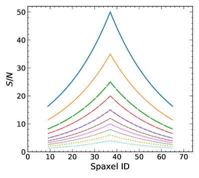
Figure 1: $S/N$ distributions used in the 1D simulations to degrade spectra in each spaxel along the major axis.

The simulations generate input rotation curves following Yoon et al. (2021),

$$V(r)=V_{c}\tanh\left(\frac{r}{R_{t}}\right)+s_{\rm out}r\,,$$ (5)

where $V_{c}=-170$ km/s, $r$ is distance from the center in spaxels, $R_{t}=7.5$ in the same units, and $s_{\rm out}=1/R_{t}=0.133$. These parameters are chosen to closely match the rotation curve reconstructed from the MaNGA 7991-12701 galaxy.

To quantify the results derived from the various fitting approaches, i.e. the output velocities for each spaxel along the 1D line of spaxels (e.g. major axis) relative to input truth, we explore the rms velocity offset and the accuracy, i.e. lack of bias. Figure 2 shows the accuracy in terms of the bias from the truth,

$$A=\frac{1}{N_{\rm fit}}\sum\frac{\Delta V_{AB}-\Delta V_{\rm true}}{\Delta V_{\rm true}}\ ,$$ (6)

for the 10 different S/N simulations of Fig. 1. The sum runs over those $N_{\rm fit}$ spaxels with at least two (of the four) wavelength regions passing the criteria in Eq. (3) with $c=1$.

Most informative is the accuracy, plotted in Figure 2 for both the iterative smoothing approach and the cubic smoothing approach. We see that the accuracy is within 1% for median $S/N$$\geq 4$ for the iterative case or 2% for median $S/N$$\geq 7$ for cubic smoothing (while the cubic smoothing approach is $\sim 25\times$ faster computationally). Recall that the median means that half of the spaxels will be lower, i.e. the median $S/N=4$ case has 50% of spaxels in $S/N=[2.3,4]$, so the technique is accurate down to quite low $S/N$. The preference for somewhat negative bias comes from that the spectral feature line widths are often comparable to the shifts induced by the rotation velocity. Thus, in the crosscorrelation between spaxels to estimate the velocity, the features may overlap, preferring lower velocity shifts than actual for low $S/N$ data that cannot resolve the line profile.

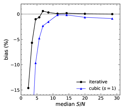
Figure 2: Reconstructed rotation curve bias relative to the simulation plotted vs median $S/N$. The black dot curve shows results for the iterative approach and the blue triangle curve is for cubic smoothing. The methods are accurate to $\lesssim 1\%$ for median $S/N\geq 4$ for iterative, and $\lesssim 2\%$ for median $S/N\gtrsim 7$ for cubic approaches.

The reconstruction techniques also provide reasonable rms velocity uncertainties, shown in Figure 3. As expected, the velocity estimation has larger uncertainties in the low$S/N$ regions, generally at the edges of a galaxy where the fractional uncertainty will still be reasonable, e.g. $\sim 10\%$. One can ameliorate the increase in velocity uncertainty by restricting to spaxels with $S/N>4$, say; we see this reduces the uncertainty by $\sim 30-40\%$ even for median $S/N\approx 3$. In the next section, we will also introduce the anchor procedure to improve robustness further.

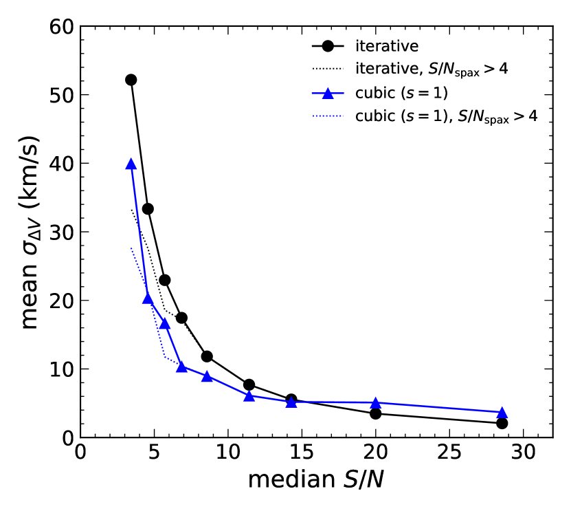
Figure 3: Rms velocity differences plotted vs median $S/N$ for the iterative (black dot curve) and cubic smoothing (blue triangle curve) approaches. Neglecting spaxels with spectra having $S/N\leq 4$ improves the rms by $\sim 30\%$ at low median $S/N$.

The cubic smoothing approach is seen to be a viable second technique. (Note the reduced rms is just due to somewhat fewer bins than in the iterative case passing the criteria and being included, with the good bins having less scatter.) Meanwhile, the iterative approach has been further established with tests beyond Bag et al. (2022). We therefore now proceed to using both approaches on actual data.

4 Application to Real Data

We wish to use all the spectral data from the integral field spectroscopy, so we extend from the 1D major axis selection previously used to the full 2D hexagon of the MaNGA field. We focus on the MaNGA 7991-12701 galaxy whose major axis only was fit in Bag et al. (2022).

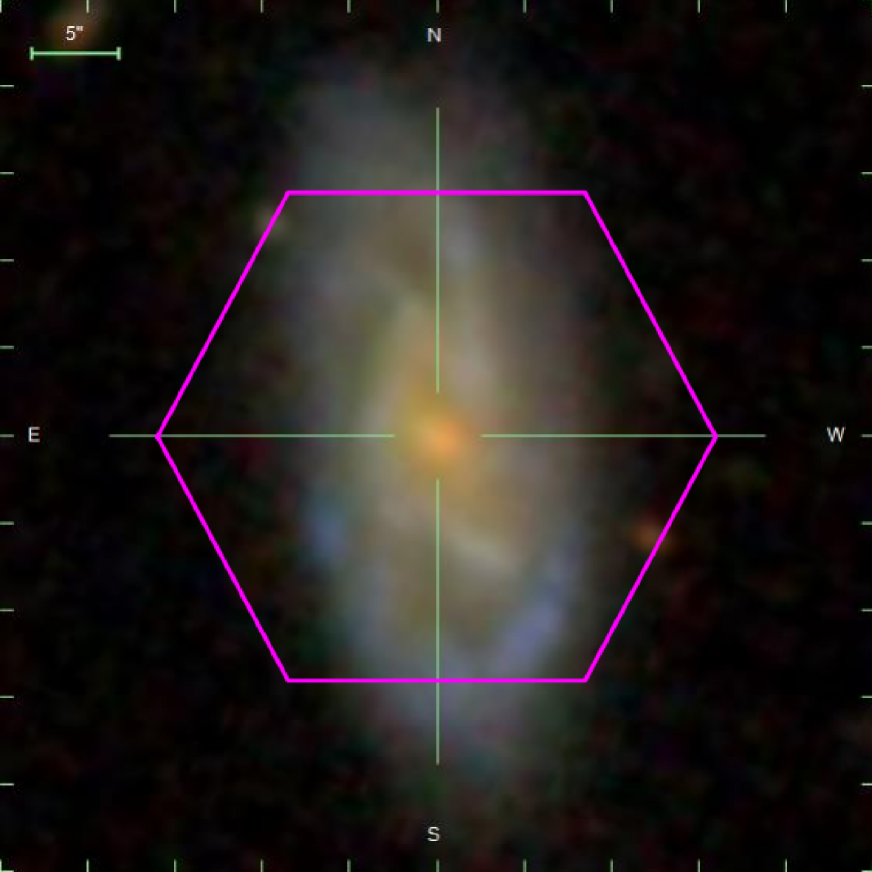
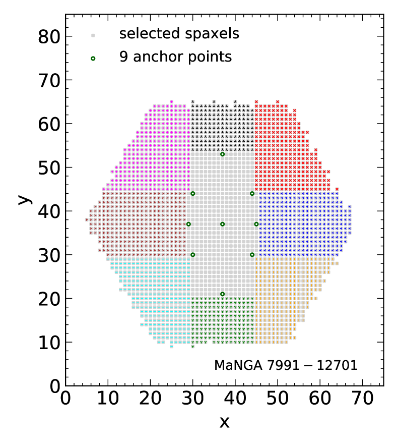
Figure 4: [Left] The optical image of the MaNGA 7991-12701 galaxy is overlaid with the hexagon of the integral field spectrograph. [Right] The spaxels are shown and our nine anchor points indicated, along with the spaxel patches (colored regions) associated to each.

MaNGA data for this galaxy comprises 2939 spaxels, but some of these have large gaps in wavelength coverage that can make the crosscorrelation technique fail or give spurious results. We remove spaxels with data at fewer than 3780 wavelengths, leaving 2632 spaxels.

If one crosscorrelated every spaxel with every other one, this would lead to the computationally challenging task of optimizing over a million correlation functions. Instead we take two approaches. One is to crosscorrelate every spaxel with the central (usually the highest $S/N$ spaxel), giving a $N_{\rm spaxel}$ rather than $N^{2}_{\rm spaxel}$ problem, but losing information on spectral variations away from the center. The second is to choose a modest set of anchor points throughout the galaxy, and define neighboring patches of spaxels “belonging” to an anchor point.

Furthermore, one aspect of real data is that the spectral properties can differ from the center of the galaxy to its edges. A variety of such spectra were investigated in Bag et al. (2022), to see the extent to which the technique there could still succeed. Here, the anchor method uses the spectra of the anchor spaxel associated with the spaxel’s patch to estimate velocity differences, rather than always using the central spaxel spectrum.

Figure 4 shows the selection of nine anchor points: one is located at the galaxy center and eight anchors are distributed in pairs along the galaxy major and minor axes and two main diagonals. We choose anchor spaxel distances from the center to maximize the number of their wavelength bins passing the velocity criteria Eq. (3), i.e. basically the anchor spectra should have good $S/N$. For the specific case of MaNGA 7991-12701, the anchors are $\pm 16$ ($\pm 8$) spaxels away from the center along the major (minor) axes and $\pm 7$ ($\pm 7$) spaxels away along the diagonal with a positive (negative) slope.

Thus, we show results for fits relative to the center (e.g. iterative: center), and using anchors (e.g. iterative: anchors), where a spaxel velocity relative to the anchor is then propagated to the velocity relative to the center through vector addition to the anchor-center velocity.

In this article, we compare these two techniques for determining the velocity map, in a local approach (1 spaxel to 1 center spaxel for the center technique, 1 spaxel to 1 anchor spaxel to 1 center spaxel for the anchor technique). The anchor technique could also be quite useful in a global fit where the optimization is carried out over all spaxels simultaneously. For nine patches (see Figure 4), and optimization within each patch independently, this would give roughly $9(N_{\rm spaxel}/9)^{2}$ correlations. Hamiltonian Monte Carlo analysis is a possibility for such 2D simultaneous optimization, but such work is beyond the scope of this article.

Carrying out the analysis of the data, we find the anchor technique shows improved results for the low $S/N$ cases. Figure 5 plots the success of velocity fits across all wavelength bins, or a subset, vs $S/N$. Note that 78% of spaxels with any $S/N$ have two or more bins passing the criteria Eq. (3), hence suitable for use in the velocity reconstruction. Looking at the range $S/N\geq 4$, we see the number of cases not passing in at least two bins (i.e. the blue and black bars) rapidly diminishes (indeed $\gtrsim 96\%$ pass). The anchor technique works even better, especially at low $S/N$, as seen by the increased height of the gold bars (all four bins pass) and diminished contribution of the blue and black bars (only one or zero bins pass).

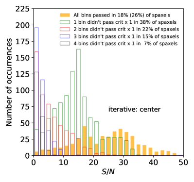
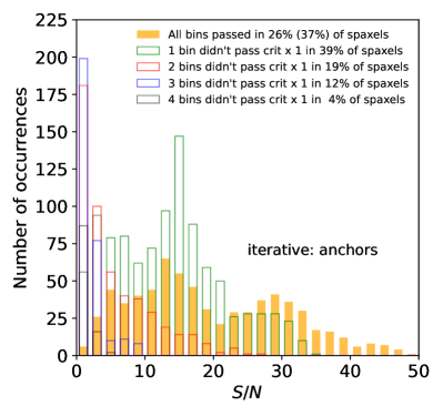
Figure 5: Distributions of signal-to-noise ratios in the MaNGA galaxy 7991–12701 spaxels, characterized by the number of bins satisfying the crit x 1 requirement on the velocity differences obtained using the iterative approach relative to the central spaxel (left), and relative to the anchor spaxels (right). For all bins passed case, the percent in parentheses is when considering only $S/N>4$.

Figure 6 summarizes the cumulative, and differential, fraction of spaxels that pass the required criteria (in at least two wavelength bins) as a function of $S/N$. We clearly see the advantage of the anchor technique, where 90% of spaxels pass even if they have only $S/N=4-5$. The more computationally efficient cubic smoothing approach also does well. When considering all spaxels with $S/N$$\geq 4$, the cubic plus anchor technique achieves 95% success.

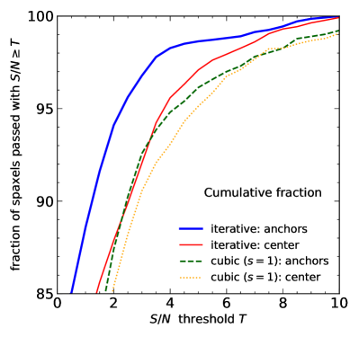
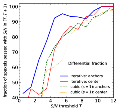
Figure 6: Cumulative fraction of spaxels with signal-to-noise ratios $S/N\geq T$ (left) and differential fraction of spaxels with signal-to-noise ratios $S/N$ in intervals $[T,T+1)$ are plotted vs the threshold $T$. Solid (dashed) curves show results for the iterative (cubic smoothing) approaches; thick (thin) curves show results via the anchor (central) spaxel technique.

We can also study how well spaxels pass the criteria, i.e. can we tighten it, or which spaxels that failed will pass if we loosen it. Adjusting the scaling factor $c$ in Eq. (3), we map in Figure 7 the velocity determination success as a function of $c$. Remarkably, the great majority of spaxels would pass for the anchor technique even if the criteria were tightened. Those that only pass with looser criteria ($c>1.25$ here) are those on the edges, far from the major axis of the galaxy, where the $S/N$ is lowest.

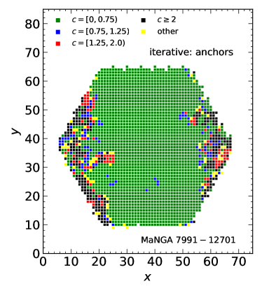
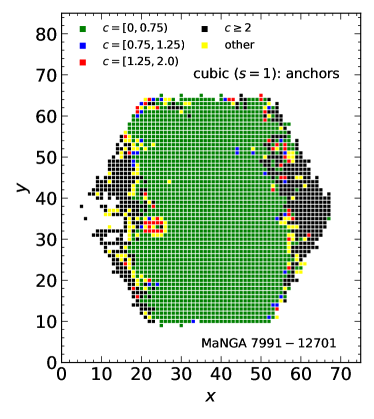
Figure 7: Success in meeting the robustness criterion for real data is shown for the 2D array of MaNGA spaxels. The color code corresponds to spaxels satisfying the criterion crit $\times\,c$ in at least two wavelength bins, for $c<0.75$, $0.75\leq c<1.25$, $1.25\leq c<2$, $c>2$. Results are given for the iterative (cubic smoothing) approach in the left (right) panel, both using the anchor technique. Yellow points indicate spaxels where the four bins fall into four distinct $c$ ranges.

Figure 8 presents the 2D velocity map we reconstruct (using our fiducial criteria $c=1$) from the MaNGA 7991-12701 galaxy integral field spectroscopy data. Note that the full region with appreciable galaxy light (i.e. nonnegligible $S/N$) is fit; only the right and left edges where the $S/N$ is very low and does not pass the robustness criteria. Iterative and cubic smoothing techniques give consistent results, though iterative succeeds to lower $S/N$.

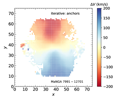
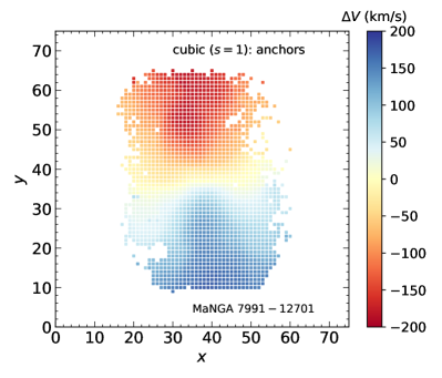
Figure 8: 2D maps of the velocity $\Delta V$ relative to the center for the MaNGA 7991-12701 galaxy for the iterative (left) and cubic smoothing (right) approaches, using the anchor technique. The standard criteria $c=1$ in at least two wavelength bins are used.

The 2D velocity map contains considerable useful information but it is often condensed to a 1D galaxy rotation curve. One can do this by assuming a particular model profile and fitting to the data, however we wish to pursue a model independent approach. Here we therefore present for illustration three slices through the 2D map, along the galaxy major axis and through the diagonal anchor points. Figure 9 presents these results. The rotation curves along the main diagonals extend to different distances due to the galaxy inclination angle, therefore they have shorter tails compared to the rotation curve found along the major axis aligned in the $y$-direction.

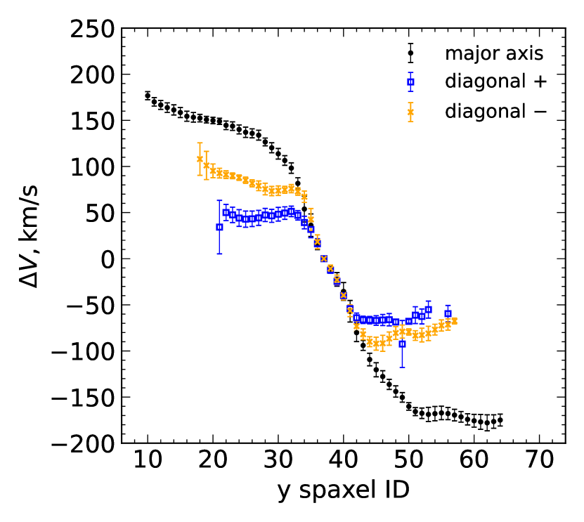
Figure 9: Reconstructed rotation curves using the iterative anchor approach along the major axis, and main diagonals with positive (negative) slope.

5 Conclusions

Integral field spectroscopy provides rich information on galaxy structure, important for the understanding of the dark matter distribution. We develop two approaches for using the full 2D array of spaxels across a galaxy to reconstruct the velocity map without assuming a profile model.

The approaches of iterative smoothing and cubic smoothing applied between two spaxels are successful at finding the relative velocity, even at low $S/N$ where standard techniques such as Penalized Pixel-Fitting (pPXF) (Cappellari & Emsellem, 2004) may have difficulty. For 90% of spaxels having as low as $S/N\in[4,5]$, for example, the fits pass our velocity estimation robustness criteria. Tests vs simulations show the velocity reconstruction bias is less than 1% down to median $S/N=4$ (i.e. where half of the spaxels have $S/N<4$). The iterative approach is more accurate than the cubic smoothing approach, but the latter is some $25\times$ faster computationally.

The use of anchor spaxels offers several advantages. Robustness is greatly improved: $\sim 90\%$ of fit spaxels pass the criteria vs $\sim 60\%$ without anchoring, and $\sim 4\times$ more spaxels pass in all wavelengths bins, for $S/N\in[4,5]$. Accuracy of the overall velocity map, i.e. recovery of input in simulations, improves. For actual data with heterogeneity of spectra across the galaxy, a spaxel is likely to have a spectrum more similar to its neighbor anchor spaxel than to the galaxy center spaxel. Finally, for eventual global fits of the velocity map, anchors and patches could reduce dimensionality of the optimization and ameliorate computational burden.

Our 2D velocity maps are smooth and well behaved, extending further off the major axis than the equivalent MaNGA-Marvin maps, and to lower $S/N$. Similarly, when projected to 1D galaxy rotation curves, the results are smoother (without any parametric model profile) and with generally smaller uncertainties. Future work includes the implementation of efficient global optimization for the maps, and further enhancement of the anchor technique.

References

- Acquaviva et al. (2012) Acquaviva V., Gawiser E., Guaita L., 2012, in Tuffs R. J., Popescu C. C., eds, The Spectral Energy Distribution of Galaxies - SED 2011 Vol. 284, The Spectral Energy Distribution of Galaxies - SED 2011. pp 42–45 (arXiv:1111.4243), doi:10.1017/S1743921312008691
- Aghamousa & Shafieloo (2015) Aghamousa A., Shafieloo A., 2015, Astrophys. J., 804, 39
- Aurenhammer (1991) Aurenhammer F., 1991, ACM Comput. Surv., 23, 345–405
- Babcock (1939) Babcock H. W., 1939, Lick Observatory Bulletin, 498, 41
- Bag et al. (2022) Bag S., Shafieloo A., Smith R., Chung H., Linder E. V., Park C., Abylkairov Y. S., Yelshibekov K., 2022, Monthly Notices of the Royal Astronomical Society, 514, 2278
- Bertone & Hooper (2018) Bertone G., Hooper D., 2018, Reviews of Modern Physics, 90, 045002
- Boquien et al. (2019) Boquien M., Burgarella D., Roehlly Y., Buat V., Ciesla L., Corre D., Inoue A. K., Salas H., 2019, A&A, 622, A103
- Bosma (1981) Bosma A., 1981, AJ, 86, 1825
- Bosma (2023) Bosma A., 2023, arXiv e-prints, p. arXiv:2309.06390
- Bryant et al. (2016) Bryant J. J., et al., 2016, in Evans C. J., Simard L., Takami H., eds, Society of Photo-Optical Instrumentation Engineers (SPIE) Conference Series Vol. 9908, Ground-based and Airborne Instrumentation for Astronomy VI. p. 99081F (arXiv:1608.03921), doi:10.1117/12.2230740
- Bundy et al. (2015) Bundy K., et al., 2015, ApJ, 798, 7
- Cappellari (2017) Cappellari M., 2017, MNRAS, 466, 798
- Cappellari & Copin (2003) Cappellari M., Copin Y., 2003, MNRAS, 342, 345
- Cappellari & Emsellem (2004) Cappellari M., Emsellem E., 2004, PASP, 116, 138
- Cid Fernandes et al. (2005) Cid Fernandes R., Mateus A., Sodré L., Stasińska G., Gomes J. M., 2005, MNRAS, 358, 363
- Cole et al. (1994) Cole S., Aragon-Salamanca A., Frenk C. S., Navarro J. F., Zepf S. E., 1994, MNRAS, 271, 781
- Croom et al. (2021) Croom S. M., et al., 2021, MNRAS, 505, 991
- Drory et al. (2015) Drory N., et al., 2015, AJ, 149, 77
- Faber & Jackson (1976) Faber S. M., Jackson R. E., 1976, ApJ, 204, 668
- Ferreras et al. (2019) Ferreras I., et al., 2019, MNRAS, 489, 608
- García-Lorenzo et al. (2015) García-Lorenzo B., et al., 2015, A&A, 573, A59
- Ge et al. (2021) Ge J., Mao S., Lu Y., Cappellari M., Long R. J., Yan R., 2021, MNRAS, 507, 2488
- Gudehus (1973) Gudehus D. H., 1973, AJ, 78, 583
- Johnson et al. (2021) Johnson B. D., Leja J., Conroy C., Speagle J. S., 2021, ApJS, 254, 22
- Koleva et al. (2009) Koleva M., Prugniel P., Bouchard A., Wu Y., 2009, Astron. Astrophys., 501, 1269
- Kretschmer et al. (2021) Kretschmer M., Dekel A., Freundlich J., Lapiner S., Ceverino D., Primack J., 2021, MNRAS, 503, 5238
- Loubser et al. (2020) Loubser S. I., Babul A., Hoekstra H., Bahé Y. M., O’Sullivan E., Donahue M., 2020, MNRAS, 496, 1857
- Ocvirk et al. (2006) Ocvirk P., Pichon C., Lançon A., Thiébaut E., 2006, MNRAS, 365, 46
- Oort (1932) Oort J. H., 1932, Bull. Astron. Inst. Netherlands, 6, 249
- Roberts & Rots (1973) Roberts M. S., Rots A. H., 1973, A&A, 26, 483
- Roberts-Borsani et al. (2020) Roberts-Borsani G. W., Saintonge A., Masters K. L., Stark D. V., 2020, MNRAS, 493, 3081
- Rubin & Ford (1970) Rubin V. C., Ford W. Kent J., 1970, ApJ, 159, 379
- Rubin et al. (1978) Rubin V. C., Ford W. K. J., Thonnard N., 1978, ApJ, 225, L107
- Rubin et al. (1980) Rubin V. C., Ford W. K. J., Thonnard N., 1980, ApJ, 238, 471
- Sánchez et al. (2012) Sánchez S. F., et al., 2012, A&A, 538, A8
- Sánchez et al. (2016a) Sánchez S. F., et al., 2016a, Rev. Mex. Astron. Astrofis., 52, 171
- Sánchez et al. (2016b) Sánchez S. F., et al., 2016b, A&A, 594, A36
- Scott et al. (2018) Scott N., et al., 2018, MNRAS, 481, 2299
- Shafieloo (2007) Shafieloo A., 2007, Mon. Not. Roy. Astron. Soc., 380, 1573
- Shafieloo & Clarkson (2010) Shafieloo A., Clarkson C., 2010, Phys. Rev. D, 81, 083537
- Shafieloo et al. (2006) Shafieloo A., Alam U., Sahni V., Starobinsky A. A., 2006, Mon. Not. Roy. Astron. Soc., 366, 1081
- Sofue & Rubin (2001) Sofue Y., Rubin V., 2001, ARA&A, 39, 137
- Stoehr et al. (2008) Stoehr F., et al., 2008, in Argyle R. W., Bunclark P. S., Lewis J. R., eds, Astronomical Society of the Pacific Conference Series Vol. 394, Astronomical Data Analysis Software and Systems XVII. p. 505
- Thomas et al. (2011) Thomas J., et al., 2011, MNRAS, 415, 545
- Tully & Fisher (1977) Tully R. B., Fisher J. R., 1977, A&A, 500, 105
- Virtanen et al. (2020) Virtanen P., et al., 2020, Nature Methods, 17, 261
- Wake et al. (2017) Wake D. A., et al., 2017, AJ, 154, 86
- Walcher et al. (2006) Walcher C. J., Boker T., Charlot S., Ho L. C., Rix H.-W., Rossa J., Shields J. C., van der Marel R. P., 2006, Astrophys. J., 649, 692
- Yan et al. (2016) Yan R., et al., 2016, AJ, 152, 197
- Yoon et al. (2021) Yoon Y., Park C., Chung H., Zhang K., 2021, The Astrophysical Journal, 922, 249
- Zwicky (1933) Zwicky F., 1933, Helvetica Physica Acta, 6, 110
- van Albada et al. (1985) van Albada T. S., Bahcall J. N., Begeman K., Sancisi R., 1985, ApJ, 295, 305