Aspects of Non-Relativistic Quantum Field Theories

Abstract

Non-relativistic quantum field theory is a framework that describes systems where the velocities are much smaller than the speed of light. A large class of those obey Schrödinger invariance, which is the equivalent of the conformal symmetry in the relativistic world. In this review, we pedagogically introduce the main theoretical tools used to study non-relativistic physics: null reduction and $c\rightarrow\infty$ limits, where $c$ is the speed of light. We present a historical overview of non-relativistic wave equations, Jackiw-Pi vortices, the Aharonov-Bohm scattering, and the trace anomaly for a Schrödinger scalar. We then review modern developments, including fermions at unitarity, the quantum Hall effect, off-shell actions, and a systematic classification of the trace anomaly. The last part of this review is dedicated to current research topics. We define non-relativistic supersymmetry and a corresponding superspace to covariantly deal with quantum corrections. Finally, we define the Spin Matrix Theory limit of the AdS/CFT correspondence, which is a non-relativistic sector of the duality obtained via a decoupling limit, where a precise matching of the two sides can be achieved.

1 Introduction and outline

Non-relativistic theories received a lot of attention since the early days of physics due to their success in explaining most of the phenomena in Nature that can be experienced in our everyday life. It was only discovered in the last century that the laws of physics were fundamentally Lorentz-invariant and that general relativity was needed to fully account for the observations in our Universe. Despite this revolutionary change, non-relativistic theories continued to play an important role in the last century, mainly to describe phenomena happening at low energies (or speed) and to study applications to condensed matter systems. The topic experienced a recent revival, starting with the seminal work by Son and Wingate on non-relativistic conformal invariance Son:2005rv . Their primary goal was the study of condensed matter systems, such as fermions at unitarity and the quantum Hall effect, that are invariant under a non-Lorentzian symmetry group and do not have a small parameter that can be used to define a perturbative expansion. Following these ideas, several theoretical investigations of non-relativistic theories have been performed in the last decades. A nice collection of reviews that cover these developments is Oling:2022fft ; Hartong:2022lsy ; Bergshoeff:2022eog ; Grosvenor:2021hkn . While they provide an extensive analysis of gravity, string theory, non-Lorentzian symmetry algebras, particle actions and applications to fractons, a review specifically devoted to non-relativistic quantum field theory (QFT) is still missing in the literature. Our goal is to fill the gap with the present paper.

The concept of non-relativistic theory is very broad. While it usually refers to systems whose symmetry group is Galilei instead of Lorentz, sometimes this terminology is also adopted to describe theories invariant under Lifshitz transformations

$$t^{\prime}=e^{z\sigma}t\,,\qquad x^{\prime}_{i}=e^{\sigma}x_{i}\,,$$ (1)

where $\sigma$ is a constant parameter, while $z$ is called dynamical exponent and characterizes the anisotropy between the rescaling of space and time. In this review, we will mainly focus on the choice $z=2$, when the symmetries can be enhanced to the Schrödinger group, which leaves the Schrödinger equation invariant. One convenient method to derive Schrödinger-invariant theories is to perform a dimensional reduction along the null direction of a relativistic theory defined on a Lorentzian manifold with null isometry (this procedure is called null reduction) Duval:1984cj . This technology will be extensively used in the present review to find an off-shell formulation for several non-relativistic models. Other ways to generate non-relativistic theories from a relativistic parent consist of performing a limit $c\rightarrow\infty$ (where $c$ is the speed of light), or an expansion in powers of $c^{-2}$. The reader can find a detailed treatment of the latter approach applied to gravity in the review Hartong:2022lsy , while in this paper we will discuss the $c\rightarrow\infty$ limit and sometimes adopt it to build non-relativistic QFTs.

The main reason to study non-relativistic systems using a QFT formulation is that is that a joined framework will allow to share methods and insights between the relativistic and non-relativistic communities. Furthermore, QFT provides a theoretical setting where several more methods, compared to QM, are available. In section 2, we motivate the above-mentioned advantages and we introduce the basic ingredients necessary to study Schrödinger-invariant systems, which are the non-relativistic counterpart of conformal field theories (CFTs). We discuss the symmetry structure of the Schrödinger group, a non-relativistic version of the state/operator correspondence, the form of correlation functions and the technology to deal with loop corrections. The above-mentioned tools are sufficient to delve in section 3 into a historical overview of the older applications: the study of non-relativistic fermions, gauge fields, and anyons. This includes exact solutions to the Jackiw-Pi model, the Aharonov-Bohm scattering, and the scale anomaly for a scalar theory with quartic interactions.

Section 4 reviews the most common methods used to study non-relativistic systems in the last decade: non-relativistic limits $c\rightarrow\infty$ (section 4.2) and null reduction (section 4.3). We apply these methods in section 5 to study several problems of interest in modern physics. We begin with condensed matter applications, i.e., fermions at unitarity and the quantum Hall effect. Then we find an off-shell formulation for theories involving the non-relativistic fermions and gauge fields introduced above. We consider a deformed version of null reduction to build QFTs invariant under the SU$(1,n)$ symmetry group, which play an important role in the non-relativistic limit of $M$–theory. We discuss trace anomalies for Schrödinger-invariant field theories.

Supersymmetry (SUSY) has been studied for several years as a candidate to uncover physics beyond the Standard Model, but has not been experimentally observed so far. There are expectations that SUSY may arise as en emergent symmetry in the IR of certain systems, e.g., the tricritical Ising model FRIEDAN198537 , topological superconductors Grover:2013rc , optical lattices Yu:2010zv and many others. Therefore, one may be interested in combining SUSY with non-relativistic symmetries, which frequently arise in condensed matter physics. From a theoretical perspective, SUSY puts strict constraints on the analytic structure of the effective action, and controls the running of physical couplings along the RG flow, leading to exact results and non-renormalization theorems Grisaru:1979wc ; Seiberg:1993vc . Moreover, even if SUSY plays an indirect role in holography, most of the examples where the AdS/CFT correspondence is explicitly tested are supersymmetric. It is then natural to ask whether the above-mentioned constraints on the quantum corrections are tied to the Lorentz group, or if they can be generalized to other spacetime symmetry groups, such as the Galilean case. This topic is studied in section 6, where a superspace formulation is introduced. This tool allows for a simpler and systematic computation of the loop corrections to certain theories with super-Schrödinger invariance.

The last part of the review is devoted to a recently growing research line, i.e., the Spin Matrix Theory (SMT) limit of AdS/CFT duality, see section 7. The AdS/CFT correspondence between $\mathcal{N}=4$ super Yang-Mills (SYM) with gauge group $\mathrm{SU}(N)$ and type IIB string theory on $\mathrm{AdS}_{5}\times S^{5}$ is the best-understood example which realizes the holographic principle, promising an understanding of how gravity emerges from a fundamental quantum theory Maldacena:1997re . Evidence in favor of AdS/CFT duality has been accumulating over the last decades, including the impressive achievements of the integrability program when $N=\infty$ Minahan:2002ve ; Beisert:2003tq ; Beisert:2010jr . However, to get a full understanding of the non-perturbative regime, which includes essential objects such as black holes and D–branes, it is necessary to work at finite $N$. The SMT sectors of the AdS/CFT duality consist of decoupling limits that either approach zero-temperature critical points (in the grand-canonical ensemble), or unitarity bounds (in the microcanonical ensemble). The outcome is that several degrees of freedom of $\mathcal{N}=4$ SYM decouple, and one is restricted to a subsector of the full theory where $N$ is fixed but arbitrary, and a non-perturbative matching between the two sides can be achieved. An important feature of the SMT limit is that the resulting theories are non-relativistic.

We summarize the main points of the review and propose several future developments in section 8. Appendix A collects the conventions and a list of acronyms.

Let us conclude with some caveats. While we will incidentally discuss applications to holography in sections 5.3 and 7.7, the main focus of the review is on field-theoretical aspects. The inexpert reader can find a pedagogical introduction of the main theoretical techniques used in non-relativistic physics in sections 2 and 4. These will allow the reader to delve into the applications discussed in the remainder of the paper. Finally, we collect in table 1 a brief primer for people interested in various topics: we mark with a green check   ✔  the sections which cover some material on condensed matter physics, supersymmetry, and contemporary research developments, respectively.

Sections	Cond. matter	Supersymmetry	Current research
Preliminaries (section 2)	✔	✘	✘
Historical review (section 3)	✔	✔	✘
Modern techniques (section 4)	✔	✘	✔
Modern applications (section 5)	✔	✘	✔
Supersymmetry (section 6)	✘	✔	✔
Spin Matrix Theory (section 7)	✘	✔	✔

Table 1: Topics discussed in various sections of the review.

2 Preliminaries

In this section, we lay the foundations by introducing the key concepts that will be central throughout this review. We begin in section 2.1 by motivating the need for non-relativistic quantum field theory to overcome the limitations of quantum mechanics. We obtain via a limiting procedure the prototype of a Schrödinger-invariant QFT in flat space in section 2.2, whose symmetry group is presented in section 2.3. This structure allows to build a non-relativistic version of state/operator correspondence and to find restrictions on the form of the correlation functions, as we present in sections 2.4 and 2.5, respectively. We discuss in section 2.6 the formalism to study the quantum corrections of a Schrödinger QFT. This section is based on the material collected in the lectures Shiralectures .

2.1 Why non-relativistic quantum field theory?

QFT was born to reconcile quantum mechanics (QM) with relativity. Historically, the Klein-Gordon equation was first considered by Schrödinger in late 1925 to study the fine structure of the hydrogen atom, but this attempt failed because the spin of the electron was not properly taken into account. This is what led Schrödinger to publish his equation in 1926 as a non-relativistic approximation able to determine the Bohr energy levels of the hydrogen atom without any fine structure. Later on, Dirac formulated in 1928 a wave equation for spin one-half particles, which was consistent with special relativity and represented an extension of the Schrödinger equation. While the Dirac equation successfully combines the invariance under the Poincaré group with the axioms of quantum mechanics, the corresponding theory admits a spectrum of energies with negative modes, thus allowing particles to decay and making the system unstable. The famous resolution to this problem proposed by Dirac was the existence of a sea of electrons that already occupy the negative energy states, and that give rise to a hole whenever they are excited into a positive energy state. This observation was later supported by the discovery of antiparticles in 1931.

The previous proposal led us from a quantum description of a single relativistic particle to a theory that contains a Dirac sea with an infinite number of particles. Wigner proved in 1931 a theorem stating that all the unitary representations of the Poincaré group are infinite-dimensional. This formal result implies that an infinite number of particles is required to achieve consistency between quantum mechanics and special relativity. The consequence is that QFT assigns an operator $\phi(\vec{x})$ (called field) in the Schrödinger picture to any point $\vec{x}$ in space. In the Heisenberg picture, operators become time-dependent as

$$\phi(t,\vec{x})=e^{\frac{i}{\hbar}Ht}\phi(\vec{x})e^{-\frac{i}{\hbar}Ht}\,.$$ (2)

In this way, the positions $(t,\vec{x})$ in the spacetime become labels on operators and they are treated on equal footing. Second quantization is the process that imposes canonical (anti)commutation relations between fields, leading to a quantum field theory. This formalism deals with observables assigned to regions of space rather than individual particles.

In this context, an important result for the consistency of QFT with QM is that quantum field theory reduces to ordinary non-relativistic quantum mechanics in a sector with fixed particle number. This can be shown as follows Srednicki:2007qs . Let us consider the Schrödinger equation in configuration space for $n$ particles with the same mass $m$ moving in an external potential $U(\vec{x})$ and interacting with each other through the potential $V(\vec{x}_{i}-\vec{x}_{j})$

$$i\hbar\frac{\partial}{\partial t}\psi=\left[\sum_{k=1}^{n}\left(-\frac{\hbar^{2}}{2m}\bigtriangleup_{k}+U(\vec{x}_{k})\right)+\sum_{k=1}^{n}\sum_{l=1}^{k-1}V(\vec{x}_{k}-\vec{x}_{l})\right]\psi\,,$$ (3)

where $\psi=\psi(t,\vec{x}_{1},\dots,\vec{x}_{n})$ is the wavefunction in position space. This is a partial differential equation that determines the complex function $\psi$.

An alternative perspective is to consider $\psi$ as a quantum field and use the abstract form of the Schrödinger equation

$$i\hbar\frac{\partial}{\partial t}\ket{\psi,t}=H\ket{\psi,t}\,,$$ (4)

which describes the evolution of a state $\ket{\psi,t}$ defined in a Hilbert space $\mathcal{H}$ under the action of the Hamiltonian operator $H$. To this aim, we introduce ladder operators satisfying the equal-time (anti)commutation relations

$$[a(\vec{x}),a(\vec{y})]_{\pm}=0\,,\qquad[a^{\dagger}(\vec{x}),a^{\dagger}(\vec{y})]_{\pm}=0\,,\qquad[a(\vec{x}),a^{\dagger}(\vec{y})]_{\pm}=\delta^{d}(\vec{x}-\vec{y})\,,$$ (5)

where $\delta^{d}(\vec{x})$ is the $d$–dimensional Dirac distribution and $\pm$ refers to either fermionic or bosonic statistics, respectively. The vacuum $\ket{0}$ of the theory is the state annihilated by all the lowering operators, i.e., $a(\vec{x})\ket{0}=0$. We define the Hamiltonian of the system

$$H\equiv\int d^{d}x\,a^{\dagger}(\vec{x})\left(-\frac{\hbar^{2}}{2m}\bigtriangleup+U(\vec{x})\right)a(\vec{x})+\frac{1}{2}\int d^{d}xd^{d}y\,a^{\dagger}(\vec{x})a^{\dagger}(\vec{y})V(\vec{x}-\vec{y})a(\vec{x})a(\vec{y})\,,$$ (6)

and a generic time-dependent multi-particle state as

$$\ket{\psi,t}\equiv\int d^{d}x_{1}\dots d^{d}x_{n}\,\psi(t,\vec{x}_{1},\dots,\vec{x}_{n})a^{\dagger}(\vec{x}_{1})\dots a^{\dagger}(\vec{x}_{n})\ket{0}\,,$$ (7)

where $\psi$ is a profile function that parametrizes a superposition between the $n$ particles. It can be proven that the Hamiltonian (6) and the state (7) satisfy the abstract Schrödinger equation (4) if and only if the wavefunction $\psi(t,\vec{x}_{1},\dots,\vec{x}_{n})$ solves the differential equation (3) in configuration space.

We can now interpret the vacuum $\ket{0}$ as a state without particles, and $\ket{\psi,t}$ defined in eq. (7) as a state with $n$ particles created at positions $\vec{x}_{1},\dots,\vec{x}_{n}$. This counting can be performed with the number operator

$$N\equiv\int d^{d}x\,a^{\dagger}(\vec{x})a(\vec{x})\,.$$ (8)

The Hamiltonian in eq. (6) satisfies $[H,N]=0$, implying that the number of particles in a state remains constant during the time evolution.

At this point, one may wonder what are the advantages of the QFT formalism, compared to QM, to describe non-relativistic phenomena. The main reason is that working in the common framework given by QFT may help us to exchange the knowledge between relativistic and non-relativistic communities for all the cases when this is relevant, e.g., to describe phenomena at low energies and when particles move at low speed. Limits usually make a system more tractable. Since non-relativistic theories can be achieved performing $c\rightarrow\infty$ limits (where $c$ is the speed of light), one may hope to get useful insights on non-relativistic systems, and then apply them to the relativistic case, too. The methods of QFT provide several technical advantages to studying the non-relativistic realm, including anomalies, computations of cross-sections and condensed-matter settings. QFT also accounts for when particles are indistinguishable. Finally, let us mention that while particle number is usually conserved in non-relativistic systems, this may not always be the case. The QFT formalism goes beyond this limitation, thus describing the phenomenology of the emission or absorption of particles.

2.2 Non-relativistic limit of quantum field theory

A simple way to generate non-relativistic QFTs is via a limiting procedure implemented on a Lorentz-invariant QFT. We will analyze in detail the modern approaches to this problem in section 4, but for the moment we review the standard approach that can be found in books (e.g., see Zee:2003mt ) and older papers Bergman:1991hf . Consider the Lagrangian for a relativistic real scalar field with quartic interaction

$$S=\int dtd^{d}x\,\mathcal{L}\,,\qquad\mathcal{L}=\frac{1}{2}(\partial_{\mu}\Phi)(\partial^{\mu}\Phi)-\frac{m^{2}}{2}\Phi^{2}-\frac{\lambda}{4!}\Phi^{4}\,,$$ (9)

where $m$ is the physical mass and $\lambda$ the coupling constant. We parametrize the relativistic scalar field as (here we insert back factors in the speed of light $c$)

$$\Phi(t,\vec{x})=\frac{1}{\sqrt{2m}}\left(e^{-imt}\varphi(t,\vec{x})+e^{imt}\varphi^{\dagger}(t,\vec{x})\right)\,.$$ (10)

So far, this is only a field redefinition, but we have in mind to interpret $\varphi,\varphi^{\dagger}$ as the non-relativistic counterparts of the original scalar field. We assume that the kinetic energy is much smaller than the rest mass, which implies $(\partial^{2}/\partial t^{2})\varphi\ll-2im(\partial/\partial t)\varphi.$ Plugging the ansatz (10) inside eq. (9) and discarding the terms which oscillate in the mass $m$ gives

$$\mathcal{L}=\varphi^{\dagger}\left(i\partial_{t}+\frac{\bigtriangleup}{2m}\right)\varphi-\frac{g}{4}|\varphi^{\dagger}\varphi|^{2}\,,$$ (11)

where $g\equiv\lambda/(4m^{2})$. This is the Lagrangian for a Schrödinger field with quartic interactions.

Let us study the classical properties of this theory. The dynamics of the scalar field $\varphi$ (and its hermitian conjugate) is given by the Schrödinger equation with a potential term. It is relevant to notice that the field $\varphi$ is complex and the Lagrangian (11) enjoys a global $\mathrm{U}(1)$ invariance. This is interpreted as the conservation of particle number (or equivalently, of the mass) and it is a distinctive feature of physical realizations of non-relativistic systems. We will see in section 2.3 that the corresponding conserved charge $N$, analogous to the number operator in eq. (8), provides a central extension of the Galilei symmetry, called the Bargmann group.

The theory (11) enjoys a larger symmetry, which includes scale invariance. Despite the explicit appearance of the mass parameter $m$, this is possible because the speed of light disappears in the non-relativistic regime. For this reason, the mass is not dimensionally equivalent to an inverse length, but we have the freedom to consider $m$ as a dimensionless and independent parameter. Indeed, the length dimensions $L$ of the coordinates and of the fields in $d+1$ dimensions read

$$[t]=L^{2}\,,\qquad[\vec{x}]=L\,,\qquad[\varphi]=[\varphi^{\dagger}]=L^{\frac{d}{2}}\,,\qquad[m]=[g]=L^{0}\,.$$ (12)

The crucial novelty, compared to the relativistic case, is that the time coordinate scales twice as much as the spatial one. This is a special case of the Lifshitz transformations (1).

It turns out that the symmetry structure of the Lagrangian (11) is even larger, comprising the invariance under the following transformations:

$$\begin{cases}t\rightarrow t+\xi^{t}&\mathrm{time\,\,translations}\\ x^{i}\rightarrow x^{i}+\xi^{i}&\mathrm{spatial\,\,translations}\\ x^{i}\rightarrow x^{i}+R^{i}_{\,\,j}x^{j}&\mathrm{spatial\,\,rotations}\\ x^{i}\rightarrow x^{i}+v^{i}t&\mathrm{Galilean\,\,boosts}\\ t\rightarrow e^{2\sigma}t\,,\quad x_{i}\rightarrow e^{\sigma}x_{i}&\mathrm{dilatations}\\ t\rightarrow\frac{t}{1+\eta t}\,,\quad x^{i}\rightarrow\frac{x^{i}}{1+\eta t}&\mathrm{special\,\,conformal\,\,transf.\,\,(\mathrm{SCT})}\end{cases}$$ (13)

Correspondingly, the Schrödinger field transforms as

$$\begin{cases}\varphi\rightarrow e^{im\vec{v}\cdot R\vec{x}+\frac{i}{2}m\vec{v}^{2}t}\,\varphi&\mathrm{Galilean\,\,transformations}\\ \varphi\rightarrow e^{-dt}\,\varphi&\mathrm{dilatations}\\ \varphi\rightarrow\left(1-\eta t\right)^{d}e^{\frac{i}{2}\frac{m\eta\vec{x}^{2}}{1-\eta t}}\,\varphi&\mathrm{SCT}\\ \varphi\rightarrow e^{i\alpha}\,\varphi\,,\quad\varphi^{\dagger}\rightarrow e^{-i\alpha}\,\varphi^{\dagger}&\mathrm{U(1)\,\,particle\,\,number}\end{cases}$$ (14)

where $R$ is a rotation matrix and the Galilean transformations in eq. (14) include translations, rotations and boosts. The full set of transformations listed above generates the so-called Schrödinger group, which can be thought of as a non-relativistic analog of the conformal group. We will sometimes refer to a QFT invariant under the Schrödinger group as a non-relativistic conformal field theory (NRCFT). We analyze the conserved charges, their Lie brackets, and the embedding inside the conformal group in section 2.3.

2.3 The Schrödinger group

The prototype of a non-relativistic theory described by a second-quantized Schrödinger field $\psi_{\alpha}(\vec{x})$, where $\alpha$ labels a representation of the spin group, is given by the action

$$S= \int dt\,d^{d}x\,\psi^{\dagger}_{\alpha}(t,\vec{x})\left(i\partial_{t}+\frac{\bigtriangleup}{2m}\right)\psi_{\alpha}(t,\vec{x})$$ (15)

$$-\frac{1}{2}\int dt\,d^{d}xd^{d}y\,\psi^{\dagger}_{\alpha}(t,\vec{x})\psi^{\dagger}_{\beta}(t,\vec{y})V(\vec{x}-\vec{y})\psi_{\beta}(t,\vec{y})\psi_{\alpha}(t,\vec{x})\,.$$

This expression generalizes eq. (11), which is recovered in the case of a $\delta$–like potential $V(\vec{x}-\vec{y})\propto\delta^{d}(\vec{x}-\vec{y})$. We assume that the fields satisfy the (anti)commutation relations

$$[\psi_{\alpha}(\vec{x}),\psi^{\dagger}_{\beta}(\vec{y})]_{\pm}=\delta^{d}(\vec{x}-\vec{y})\,\delta_{\alpha\beta}\,.$$ (16)

The Noether charges generating the transformations (13) and (14) read Hagen:1972pd

$$H=\frac{1}{2m}\int d^{d}x\,\partial_{i}\psi^{\dagger}_{\alpha}(\vec{x})\partial_{i}\psi_{\alpha}(\vec{x})+\frac{1}{2}\int d^{d}xd^{d}y\,\psi^{\dagger}_{\alpha}(\vec{x})\psi^{\dagger}_{\beta}(\vec{y})V(\vec{x}-\vec{y})\psi_{\beta}(\vec{y})\psi_{\alpha}(\vec{x})\,,$$ (17)

$$P_{i}=\int d\vec{x}\,j_{i}(\vec{x})\,,\qquad J_{ij}=\int d\vec{x}\left(x_{i}j_{j}(\vec{x})-x_{j}j_{i}(\vec{x})\right)\,,\qquad G_{i}=\int d\vec{x}\,x_{i}n(\vec{x})\,,$$

$$M=mN=m\int d\vec{x}\,n(\vec{x})\,,\qquad D=-\int d\vec{x}\,x_{i}j_{i}(\vec{x})\,,\qquad C=\int d\vec{x}\,\frac{\vec{x}^{2}}{2}n(\vec{x})\,,$$

where the number and momentum density are defined as

$$n(\vec{x})=\psi^{\dagger}_{\alpha}(\vec{x})\psi_{\alpha}(\vec{x})\,,\qquad j_{i}(\vec{x})=-\frac{i}{2}\left(\psi^{\dagger}_{\alpha}(\vec{x})\partial_{i}\psi_{\alpha}(\vec{x})-\partial_{i}\psi^{\dagger}_{\alpha}(\vec{x})\psi_{\alpha}(\vec{x})\right)\,.$$ (18)

The currents (18) satisfy the continuity equation $\partial_{t}n+\partial_{i}j_{i}=0.$ We associate the symmetry transformations with the corresponding conserved charges in table 2. The generators satisfy the following Lie brackets (all the other commutators vanish)

$$[J^{ij},J^{kl}]=i\left(\delta^{ik}J^{jl}+\delta^{jl}J^{ik}-\delta^{il}J^{jk}-\delta^{jk}J^{il}\right)\,,$$ (19)

$$[J^{ij},P^{k}]=i\left(\delta^{ik}P^{j}-\delta^{jk}P^{i}\right)\,,\qquad[J^{ij},G^{k}]=i\left(\delta^{ik}G^{j}-\delta^{jk}G^{i}\right)\,,$$

$$[D,P^{i}]=iP^{i}\,,\qquad[D,G^{i}]=-iG^{i}\,,\qquad[D,H]=2iH\,,\qquad[D,C]=-2iC\,,$$

$$[H,G^{i}]=-iP^{i}\,,\qquad[H,C]=-iD\,,\qquad[P^{i},G^{j}]=-i\delta^{ij}M\,,$$

composing the Schrödinger algebra. The mass generator is a central charge of the algebra, since it commutes with all the other generators. Since $[H,M]=[H,N]=0,$ the mass (and the particle number) is conserved in a physical theory invariant under the Schrödinger symmetry. The subset $\{H,P_{i},J_{ij},G_{i},M\}$ composes the Bargamann subalgebra, which is a central extension of the Galilean algebra. The Schrödinger group is the largest group of (bosonic) symmetries of the Schrödinger equation. It can be obtained via an Inonü-Wigner contraction, corresponding to the non-relativistic limit $c\rightarrow\infty$, of the $\mathrm{U}(1)$ centrally extended conformal group.

Transformations	Generators
Time translations	Hamiltonian $H$
Spatial translations	Momenta $P_{i}$
Spatial rotations	Angular momenta $J_{ij}$
Galilean boosts	Generators $G_{i}$
$\mathrm{U(1)}$ internal symmetry	Mass $M$
Scale transformations	Dilatation operator $D$
SCT	Generator $C$

Table 2: Conserved charges (right column) in eq. (17) generating the transformations of the Schrödinger group listed in the left column.

In the relativistic case, an open problem is the relation between scale and conformal symmetry, e.g., see Nakayama:2013is for a review. There are several hints to believe that unitary plus scale invariance, together with other technical assumptions, imply conformal invariance. The validity of this statement was also proven in two and four dimensions Polchinski:1987dy ; Dymarsky:2013pqa . It is natural to ask whether the same relation exists between scale and Schrödinger invariance, since the latter can be thought as the non-relativistic counterpart of conformal symmetry. First of all, let us comment that the Lifshitz algebra, which is associated to the dilatations (1), does not contain any special conformal transformation. Therefore, this example provides a class of non-Lorentzian theories where the enhancement is not possible, simply because it cannot exist. Instead, the non-trivial issue is the possibility to enhance Galilean plus scale invariance into the Schrödinger symmetry. To begin with, one can show that the Ward identity associated with Schrödinger invariance implies

$$2T^{00}-\delta_{ij}T^{ij}=0\,,$$ (20)

where the components of the stress tensor are specified below. More precisely, we define

$$H=\int d^{d}x\,T^{00}\,,\qquad P^{i}=\int d^{d}x\,T^{0i}\,,$$ (21)

while the spatial components $T_{ij}$ of the energy-momentum tensor satisfy the conservation equation $\partial_{t}j_{i}+\partial_{j}T_{ij}=0$, where the previous currents and charges were defined in eqs. (17) and (18). We do not report here $T_{ij}$ because its explicit expression is cumbersome and not required for the following discussion.

At this point, it was argued in Nakayama:2009ww that any stress tensor whose trace satisfies

$$2T^{00}-\delta_{ij}T^{ij}=\partial_{t}S+\partial_{i}A^{i}\,,$$ (22)

corresponds to a scale-invariant theory with dilatation operator

$$D=\int d^{d}x\,\left(tT^{00}-\frac{1}{2}x_{i}T^{0i}-\frac{S}{2}\right)\,.$$ (23)

One can further show that a stress tensor of the form (22) can be improved to be traceless if $S=\partial_{i}\sigma^{i}$, in which case one can indeed build a conserved current associated to SCTs. When this improvement is possible, scale and Galilean invariance leads to Schrödinger symmetry. This topic is still subject of research studies.

In the next subsection, we analyze the consequences of the Schrödinger symmetry on the operator product expansion (OPE) and the correlation functions of a theory.

2.4 Non-relativistic state/operator correspondence

A powerful tool in CFT is the state/operator correspondence, which relates

$$\mathrm{local\,\,operators\,\,on}\,\,\mathbb{R}^{D}\quad\Leftrightarrow\quad\mathrm{states\,\,on\,\,}S^{D-1}\,.$$ (24)

This is possible due to the conformal mapping between the Euclidean plane $\mathbb{R}^{D}$ and the cylinder $\mathbb{R}\times S^{D-1}$, up to a conformal factor:

$$ds^{2}=d\rho^{2}+\rho^{2}d\Omega_{D-1}^{2}\quad\underset{\rho=e^{\tau}}{\longrightarrow}\quad ds^{2}=e^{2\tau}\left(d\tau^{2}+d\Omega_{D-1}^{2}\right)\,.$$ (25)

This transformation maps the dilatation operator $D=\rho\partial_{\rho}$ on the plane to the Hamiltonian $H=\partial_{\tau}$ on the cylinder. On $\mathbb{R}\times S^{D-1},$ boundary conditions are chosen at the Euclidean time $\tau=-\infty$ to prepare a state at $\tau=0$. The space is foliated by time slices and this setting is called state picture. After the conformal transformation to the plane, the boundary conditions are mapped to the insertion of a local operator at $\rho=0$, while the state is now prepared at the sphere located at $\rho=1$. The dilatation operator naturally foliates the space into radial slices, and this setting is called operator picture. The relation between the states created on the cylinder and the insertion of an operator at the origin is the realization of the state/operator correspondence. The essential features defining this relation are

• The identification between the energy eigenvalues of the Hamiltonian in the state picture and the scaling dimensions of the corresponding operators.

• The bijective map between the cylinder and the Euclidean plane.

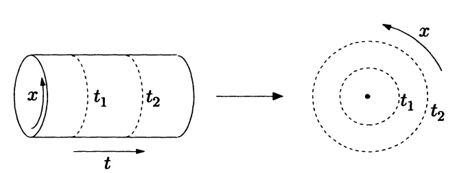
Figure 1: Conformal mapping between $\mathbb{R}\times S^{D-1}$ (left) and $\mathbb{R}^{D}$ (right). The foliation induced by the time coordinate on the cylinder corresponds to a radial foliation on the Euclidean plane. Picture taken from DiFrancesco:1997nk .

It is natural to ask whether the state/operator correspondence also applies to the non-relativistic case. The bijective map between two geometries with non-relativistic isometries is a non-trivial task and is the subject of ongoing research, as we will mention in section 5.6. Here we review the identification between the eigenvalues of a certain Hamiltonian and the dilatation operator Nishida:2007pj . Local operators $\mathcal{O}(t,\vec{x})$ in the Heisenberg picture can be defined at any point in spacetime in terms of operators inserted at the origin $\mathcal{O}(0)$ as

$$\mathcal{O}(t,\vec{x})=e^{i(Ht-P_{i}x^{i})}\mathcal{O}(0)e^{-i(Ht-P_{i}x^{i})}\,.$$ (26)

The subgroup of the Schrödinger group which leaves invariant the origin corresponds to spatial rotations, the $U(1)$ global symmetry, dilatations, and SCTs. The local operators at the origin form a representation of the reduced algebra. We declare that the scaling dimension $\Delta_{\mathcal{O}}$ and the mass eigenvalue $M_{\mathcal{O}}$ are given by

$$[D,\mathcal{O}(0)]=i\Delta_{\mathcal{O}}\mathcal{O}(0)\,,\qquad[M,\mathcal{O}(0)]=M_{\mathcal{O}}\mathcal{O}(0)\,.$$ (27)

The scaling dimension of local operators can be raised or lowered with the following generators

$$[D,[P_{i},\mathcal{O}(0)]]=i\left(\Delta_{\mathcal{O}}+1\right)[P_{i},\mathcal{O}(0)]\,,\qquad[D,[G_{i},\mathcal{O}(0)]]=i\left(\Delta_{\mathcal{O}}-1\right)[G_{i},\mathcal{O}(0)]\,,$$ (28)

$$[D,[H,\mathcal{O}(0)]]=i\left(\Delta_{\mathcal{O}}+2\right)[H,\mathcal{O}(0)]\,,\qquad[D,[C,\mathcal{O}(0)]]=i\left(\Delta_{\mathcal{O}}-2\right)[C,\mathcal{O}(0)]\,.$$

The lowest weights in the representation are called primary operators, satisfying

$$[G_{i},\mathcal{O}(0)]=[C,\mathcal{O}(0)]=0\,.$$ (29)

They comprise an irreducible representation of the Schrödinger algebra. The tower of descendants is obtained by acting with the Hamiltonian and momentum generators

$$[H,\mathcal{O}(0)]=i\partial_{t}\mathcal{O}(0)\,,\qquad[P_{i},\mathcal{O}(0)]=-i\partial_{i}\mathcal{O}(0)\,.$$ (30)

The above-mentioned representation structure only makes sense when the mass eigenvalue is non-vanishing, i.e., $M_{\mathcal{O}}\neq 0$. When $M_{\mathcal{O}}=0$, the Galilean algebra (19) implies $[P^{i},G^{j}]=0,$ therefore the distinction between primaries and descendants breaks down Bekaert:2011qd . In particular, if $\mathcal{O}(0)$ is primary, so is also the descendant $[P_{i},\mathcal{O}(0)]$. From now on, we will assume to work in a sector with a non-vanishing mass eigenvalue.

Now we show that each primary operator of the Schrödinger group corresponds to an energy eigenstate of the oscillator Hamiltonian Nishida:2007pj

$$H_{\rm osc}=H+C\,,$$ (31)

where we set the mass and the frequency of the oscillator to $m=\omega=1$ for convenience. This system is a harmonic oscillator because the generator $C$ of the special conformal transformation can be represented in terms of a quadratic potential, see eq. (17). Assuming that the operator $\mathcal{O}(0)$ is composed of annihilation operators, then its hermitian conjugate will act non-trivially on the vacuum $\ket{0}$, and it is possible to define the state

$$\ket{\Psi_{\mathcal{O}}}\equiv e^{-H}\mathcal{O}^{\dagger}\ket{0}\,,$$ (32)

which has mass eigenvalue $M_{\mathcal{O}^{\dagger}}.$ By direct computation, one can show that this is an eigenstate of the oscillator Hamiltonian such that

$$H_{\rm osc}\ket{\Psi_{\mathcal{O}}}=\Delta_{\mathcal{O}}\ket{\Psi_{\mathcal{O}}}\,.$$ (33)

This identifies the energy levels of an oscillator Hamiltonian as the scaling dimensions of the dilatation operator of the Schrödinger algebra. In this sense, the oscillator Hamiltonian (31) plays the same role as the radial quantization Hamiltonian in a relativistic CFT. Since the eigenstates of a harmonic oscillator are organized into ladders with raising and lowering operators $L_{\pm}=H-C\pm iD$, one can further show that the state $\ket{\Psi_{\mathcal{O}}}$ is the lowest weight of the representation, i.e.,

$$L_{-}\ket{\Psi_{\mathcal{O}}}=0\,.$$ (34)

Thus we have built a tower of states by inserting an operator at the origin and then acting with the ladder operators of the Hamiltonian for a harmonic oscillator.

2.5 Correlation functions

In a relativistic CFT, conformal symmetry uniquely fixes the form of two and three-point functions involving primary operators, while the kinematics is not sufficient to fully restrict four-point functions. In particular, there exist two conformal-invariant blocks (called cross ratios) that can be used to construct the general form of four and higher-point functions. The conformal bootstrap program is based on these facts and the idea that the OPE imposes crossing relations between correlation functions FERRARA1973161 .

Schrödinger invariance is less constraining than the conformal case, in particular only two-point functions are fixed by symmetry Goldberger:2014hca . For any set of $n$ operators, we define a correlation function as

$$G_{n}(t_{1},\vec{x}_{1};\dots;t_{n},\vec{x}_{n})\equiv\langle 0|T\mathcal{O}_{1}(t_{1},\vec{x}_{1})\dots\mathcal{O}_{n}(t_{n},\vec{x}_{n})|0\rangle\,,$$ (35)

where $T$ is the time-ordering and $\ket{0}$ is the vacuum state, annihilated by all the generators, including $M\ket{0}=0$. Since local operators are required to have definite mass eigenvalue, this implies that the $n$–point functions are non-vanishing if and only if $\sum_{i=1}^{n}M_{\mathcal{O}_{i}}=0$, where $M_{\mathcal{O}_{i}}$ are the mass eigenvalues associated to the operators $\mathcal{O}_{i}$.

Let us now focus on the correlation functions of scalar primary operators, which we denote as $\phi_{i}(t_{i},\vec{x}_{i})$. We begin with the two-point functions. Due to the condition on the mass eigenvalues, it is not restrictive to choose the operator basis such that $\phi_{2}(t,\vec{x})=\phi_{1}^{\dagger}(t,\vec{x})$. The structure of two-point functions is restricted by symmetries to the form

$$G_{2}(t_{1},\vec{x}_{1};t_{2},\vec{x}_{2})=\langle 0|T\phi_{1}(t_{1},\vec{x}_{1})\phi_{1}^{\dagger}(t_{2},\vec{x}_{2})|0\rangle=c|t_{12}|^{-\Delta_{1}}\,\exp\left(-i\frac{M_{1}}{2}\frac{\vec{x}_{12}^{2}}{t_{12}}\right)\,,$$ (36)

with the constraint $\Delta_{1}=\Delta_{2}$ on the scaling dimensions of the fields. Here $M_{1}$ denotes the mass eigenvalue of the scalar field, while $t_{12}\equiv t_{1}-t_{2}$, $\vec{x}_{12}\equiv\vec{x}_{1}-\vec{x}_{2}$.

Similar techniques can be applied to restrict the form of higher-point functions. The major difference with the relativistic case is that one can build either cross ratios involving only the time direction, or mixed combinations of time and space coordinates:

$$t_{ijkl}\equiv\frac{t_{ij}t_{kl}}{t_{il}t_{jk}}\,,\qquad(i,j,k,l=1,\dots,n)$$ (37)

$$v_{ijk}\equiv\frac{1}{2}\left(\frac{\vec{x}_{jk}^{2}}{t_{jk}}+\frac{\vec{x}^{2}_{ij}}{t_{ij}}-\frac{\vec{x}^{2}_{ik}}{t_{ik}}\right)\,,\qquad(i<j<k)$$

Since these blocks are both invariant under the Schrödinger symmetries, they can be used to build non-trivial correlation functions. The most general form of the three and four-point functions involving scalar primaries is given by Henkel:1993sg ; Volovich:2009yh

$$G_{3}(1,2,3)=F(v_{123})\,\exp\left(-i\frac{M_{1}}{2}\frac{\vec{x}_{13}^{2}}{t_{13}}-i\frac{M_{2}}{2}\frac{\vec{x}_{23}^{2}}{t_{23}}\right)\prod_{i<j}t_{ij}^{\frac{\Delta}{2}-\Delta_{i}-\Delta_{j}}\,,$$ (38)

$$G_{4}(1,2,3,4)=H(v_{124},v_{134},v_{234},t_{1234})\,\exp\left(-i\frac{M_{1}}{2}\frac{\vec{x}_{14}^{2}}{t_{14}}-i\frac{M_{2}}{2}\frac{\vec{x}_{24}^{2}}{t_{24}}-i\frac{M_{3}}{2}\frac{\vec{x}_{34}^{2}}{t_{34}}\right)\prod_{i<j}t_{ij}^{\frac{\Delta}{6}-\frac{\Delta_{i}+\Delta_{j}}{2}}\,,$$

where $\Delta\equiv\sum_{i}\Delta_{i},$ while $F,H$ are analytic functions.

Schrödinger symmetry is less constraining than its relativistic counterpart, in fact, the structure of three-point functions is not entirely fixed. For this reason, the conformal bootstrap approach is less constraining, and in general more freedom is allowed in the non-relativistic case Chen:2020vvn ; Chen:2022jhx . Relatedly, in any QFT the operator product expansion (OPE) states that products of nearby operators have an expansion in terms of local operators as

$$\lim_{t,x\rightarrow 0}\phi_{1}(t,\vec{x})\phi_{2}(0)=\sum_{\alpha}c_{\alpha}(t,\vec{x},\partial_{t},\partial_{i})\mathcal{O}(0)\,,$$ (39)

where the summation involves a sum over primaries and descendants. This is an operator equation, which holds inside correlation functions and can be used to obtain consistency conditions between different channels. The functions $c_{\alpha}$ can be determined by acting on the OPE with the generators of the non-relativistic conformal group and by exploiting the transformation properties of the operators, e.g., see Goldberger:2014hca for a concrete approach.

2.6 Quantum corrections

Next, we move to the analysis of the quantum properties of a Schrödinger-invariant field theory. While the following discussion will be general, for a concrete example we will refer to the scalar model (11). Free fields can be written in terms of a Fourier expansion

$$\varphi(t,\vec{x})=\int\frac{d^{d}k}{(2\pi)^{d}}\,a(\vec{k})e^{-i(\omega_{k}t-\vec{k}\cdot\vec{x})}\,,\qquad\varphi^{\dagger}(t,\vec{x})=\int\frac{d^{d}k}{(2\pi)^{d}}\,a^{\dagger}(\vec{k})e^{i(\omega_{k}t-\vec{k}\cdot\vec{x})}\,,$$ (40)

where $\omega_{k}\equiv\vec{k}^{2}/(2m).$ We canonically quantize the scalar fields by imposing the commutation relations

$$[\varphi(t,\vec{x}),\varphi(t,\vec{y})]=[\varphi^{\dagger}(t,\vec{x}),\varphi^{\dagger}(t,\vec{y})]=0\,,\qquad[\varphi(t,\vec{x}),\varphi^{\dagger}(t,\vec{y})]=\delta^{d}(\vec{x}-\vec{y})\,.$$ (41)

The vacuum state is annihilated by the lowering operator $a(\vec{k})\ket{0}$. The operator $a(\vec{k})$ destroys a particle with momentum $\vec{k}$, while the hermitian conjugate $a^{\dagger}(\vec{k})$ creates a particle with momentum $\vec{k}$. It is important to notice that, contrarily to the relativistic case, the Fourier expansions (40) only contain ladder operators of one kind. This is a consequence of the global $\mathrm{U}(1)$ symmetry, which implies the number of particles is conserved. After the non-relativistic limit, the anti-particles of the original QFT have decoupled and they form a separate sector of the theory.

One can study quantum corrections using standard perturbative methods as in any standard QFT. The free non-relativistic propagator reads

$$G_{2}(t,\vec{x})=\int\frac{d\omega d^{d}p}{(2\pi)^{d+1}}\frac{e^{-i(\omega t-\vec{p}\cdot\vec{x})}}{\omega-\frac{\vec{p}^{2}}{2m}+i\varepsilon}=-\frac{\Theta(t)}{(2\pi)^{d/2}}\,\exp\left(\frac{i\vec{x}^{2}}{2mt}\right)\,,$$ (42)

where $\Theta$ is the Heaviside distribution. As discussed in section 2.2 below eq. (12), the dimensional counting in a non-relativistic theory should be performed by referring to the scaling dimensions of the data under Lifshitz dilatations. In terms of the energy dimensions, for a Schrödinger-invariant theory we have

$$[\omega]=E^{2}\,,\qquad[k_{i}]=E\,,\qquad[m]=[g]=E^{0}\,.$$ (43)

The non-relativistic propagator has a retarded $i\varepsilon$ prescription which follows the order of the fields shown in eq. (47). This property will be crucial to simplify the study of loop corrections, as we will show below.

Feynman rules.

We define the generating functional

$$\mathcal{Z}[J,J^{\dagger}]=\int[\mathcal{D}\varphi\,\mathcal{D}\varphi^{\dagger}]\,\exp\left[iS+i\int dtd^{d}x\,\left(J\varphi+J^{\dagger}\varphi^{\dagger}\right)\right]\,,$$ (44)

where $S$ is the classical action for a (Schrödinger) field, while $J,J^{\dagger}$ are sources for the scalar field and its hermitian conjugate. By defining functional derivatives as

$$\frac{\delta J(t,\vec{x})}{\delta J(t^{\prime},\vec{x}^{\prime})}=\delta(t-t^{\prime})\delta^{d}(\vec{x}-\vec{x}^{\prime})\,,\qquad\frac{\delta J^{\dagger}(t,\vec{x})}{\delta J^{\dagger}(t^{\prime},\vec{x}^{\prime})}=\delta(t-t^{\prime})\delta^{d}(\vec{x}-\vec{x}^{\prime})\,,$$ (45)

we obtain the correlation functions via repeated action of the derivatives on the generating functional:

$$\langle\varphi(t_{1},\vec{x}_{1})\dots\varphi(t_{n/2},\vec{x}_{n/2})\varphi^{\dagger}(t_{n/2+1},\vec{x}_{n/2+1})\dots\varphi^{\dagger}(t_{n},\vec{x}_{n})\rangle=$$ (46)

$$=\frac{1}{\mathcal{Z}[J,J^{\dagger}]}\frac{\delta}{i\,\delta J(t_{1},\vec{x}_{1})}\dots\frac{\delta}{i\,\delta J(t_{n/2},\vec{x}_{n/2})}\frac{\delta}{i\,\delta J^{\dagger}(t_{n/2+1},\vec{x}_{n/2+1})}\dots\frac{\delta}{i\,\delta J^{\dagger}(t_{n},\vec{x}_{n})}\mathcal{Z}[J,J^{\dagger}]\Big{|}_{J=J^{\dagger}=0}\,.$$

We list the Feynman rules:

• Propagator. It is obtained by inverting the kinetic operator. For a Schrödinger scalar:

  $$\includegraphics[valign={c},scale={1}]{Figures/prop_scalar.pdf}=\langle\varphi(\omega,\vec{p})\varphi^{\dagger}(-\omega,-\vec{p})\rangle=\frac{i}{\omega-\frac{\vec{p}^{2}}{2m}+i\varepsilon}$$ (47)

  The arrow denotes the eigenvalue associated with the global $\mathrm{U(1)}$ particle number.

• Vertices. They are directly read from the action. Energy and spatial momentum are conserved at every vertex. Furthermore, in Schrödinger-invariant QFTs the $\mathrm{U}(1)$ particle number is conserved, which implies at a visual level that the number of arrows entering and exiting a vertex has to match. In the case of the theory (11), there is only the following four-point vertex, with associated coupling $g$:

  (48)

At this point, Feynman diagrams are built in the standard way:

1. Draw external lines for each ingoing and outgoing particle.

2. Connect the external lines using propagators and assign to them the corresponding energy, momentum, and $\mathrm{U}(1)$ particle number.

3. Impose conservation of energy, momentum, and particle number at each vertex.

4. Integrate over all loop momenta. Include a factor of $-1$ for each fermionic loop.

5. Draw all the topologically inequivalent graphs at the desired order.

6. Include combinatorial factors arising from the expansion of the interacting Lagrangian.

Another familiar notion from relativistic QFT is the effective action, which is the Legendre transform of the free energy. The effective action plays an important role because it is the generating functional of one-particle irreducible (1PI) diagrams, which are graphs remaining connected after cutting any of their lines. The precise relation reads

$$\langle\varphi(t_{1},\vec{x}_{1})\dots\varphi(t_{n/2},\vec{x}_{n/2})\varphi^{\dagger}(t_{n/2+1},\vec{x}_{n/2+1})\dots\varphi^{\dagger}(t_{n},\vec{x}_{n})\rangle_{\rm 1PI}=$$ (49)

$$=i\,\frac{\delta}{\delta\varphi_{0}(t_{1},\vec{x}_{1})}\dots\frac{\delta}{\delta\varphi_{0}(t_{n/2},\vec{x}_{n/2})}\frac{\delta}{\delta\varphi_{0}^{\dagger}(t_{n/2+1},\vec{x}_{n/2+1})}\dots\frac{\delta}{\delta\varphi_{0}^{\dagger}(t_{n},\vec{x}_{n})}\Gamma^{(n)}[\varphi_{0},\varphi_{0}^{\dagger}]\Big{|}_{J=J^{\dagger}=0}\,.$$

Here we denoted with $(\varphi_{0},\varphi^{\dagger}_{0})$ the classical fields, and with $\Gamma^{(n)}[\varphi_{0},\varphi_{0}^{\dagger}]$ the $k$–th order in the Taylor expansion of the effective action around the classical field configurations. With these ingredients, loop corrections to the effective action can be systematically studied.

Causal properties of the non-relativistic propagator.

Let us focus on the causal properties of the non-relativistic propagator (42). The retarder nature is responsible for the following selection rule:

Selection rule 2.1

Any 1P-irreducible Feynman diagram with a negative superficial degree of divergence in the $\omega$ variable and whose arrows form a closed loop, vanishes.

The superficial degree of divergence $\Delta_{\omega}$ is defined as the power of the $\omega$ variable at the numerator minus the power of $\omega$ at the denominator of a loop integral, including its measure. It is used to determine the UV divergence of an integrand. The arrows represent the flux of $\mathrm{U}(1)$ particle number across the diagram, and they form a closed loop when they are oriented in the same way (clockwise or counter-clockwise). To explain concretely the application of the selection rule, we consider the prototypical example represented by the one-loop correction to the self-energy for the action (11) depicted in fig. 2.

Figure 2: One-loop contribution to the self-energy of the scalar field.

We start for convenience from the case $d=2$. The relevant integral reads

$$\int\frac{d\omega d^{2}k}{(2\pi)^{3}}\,\frac{1}{\omega-\frac{\vec{p}^{2}}{2m}+i\varepsilon}\frac{1}{(\omega-\Omega)-\frac{(\vec{k}-\vec{p})^{2}}{2m}+i\varepsilon}\,,$$ (50)

whose superficial degree of divergence is $\Delta_{\omega}=-1.$ There are two ways to prove that this integral vanishes:

• Momentum space. We perform the $\omega$ integration first. Since the poles in $\omega$ are located on the same half-plane in complex space, the application of Jordan’s lemma to close the integration contour in the region without poles gives a vanishing integral by means of the residue theorem.

• Configuration space. Direct use of the expression (42) in position space leads to a product of two Heaviside step functions with opposite arguments. Since this result has support in a single point, we can impose that it vanishes by normal ordering.

The generalization of the previous argument to higher dimensions is trivial, since the identity (42) is general. The extension to generic loop integrals relies on the observation that Jordan’s lemma can be applied to any meromorphic function whose superficial degree of divergence respects $\Delta_{\omega}<0,$ which is one of the hypotheses of the selection rule. Since arrows forming a closed loop imply that the poles in $\omega$ always sit in the same half-plane, the proof follows by applying the residue theorem after choosing an integration contour located in that region of complex space. The selection rule 2.1 was initially observed in Bergman:1991hf and later applied in Klose:2006dd and in more recent works (e.g., see Auzzi:2019kdd ; Arav:2019tqm ; Chapman:2020vtn ; Baiguera:2022cbp ) to prove the existence of non-renormalization theorems, as we will discuss in sections 5.5, 6.3 and 6.4.

3 Historical review

We present a historical overview of the old developments in the realm of non-relativistic QFT, from the ’60s until the last decades. Recent methods (after the revival of the topic by Son and collaborators in 2005) and their applications will be discussed in section 4 and 5, respectively. Our journey begins in sections 3.1 and 3.2 with the non-relativistic versions of Dirac equations and electromagnetism. Particles with fractional statistics, the anyons, give rise to solvable systems when coupled with non-relativistic matter. This leads to the Jackiw-Pi model (section 3.3), the Aharonov-Bohm scattering problem (section 3.4), and the superconformal Chern-Simons theory (section 3.5). Finally, we will show in section 3.6 that non-relativistic QFT methods allow us to compute the trace anomaly for a Schrödinger scalar with quartic interaction.

3.1 Non-relativistic Dirac equation

It is often believed that spin is a property of relativistic theories and that the Dirac equation is the only framework able to reproduce the gyromagnetic ratio for a spin one-half particle. Below we review, following LvyLeblond1967NonrelativisticPA , how some of these features are valid for non-relativistic systems, too.

Non-relativistic wave equation.

By construction, the Schrödinger equation is preserved by Galilean transformations, as it was shown for scalar fields in section 2.2. To accommodate for spin, fields must transform in the following way under the Galilean transformations in eq. (13) LvyLeblond1967NonrelativisticPA ; Hagen:1972pd :

$$\psi_{\alpha}^{\prime}(t^{\prime},\vec{x}^{\prime})=e^{if(t,\vec{x})}\sum_{\beta=-s}^{s}D^{s}_{\alpha\beta}(R)\,\psi_{\beta}(t,\vec{x})\,,\qquad f(t,\vec{x})=\frac{1}{2}m\vec{v}^{2}t+m\vec{v}\cdot R\vec{x}\,,$$ (51)

where $\alpha,\beta$ are spinorial indices and $D^{s}$ is the $(2s+1)$–dimensional representation of the rotation group in Euclidean space. Eq. (51) corresponds to a unitary ray representation of the Galilei group which preserves the local probability density $|\psi_{\alpha}^{\prime}(t^{\prime},\vec{x}^{\prime})|^{2}=|\psi_{\alpha}(t,\vec{x})|^{2}$.

Next, we show that the index $s$ can be interpreted as the spin of a non-relativistic particle, starting from the case $s=1/2$. Let us search for a first-order wave equation linear in both the temporal and spatial derivatives

$$\mathcal{O}\psi\equiv\left(ia\partial_{t}+i\vec{b}\cdot\nabla+c\right)\psi=0\,,$$ (52)

where $\mathcal{O}$ denotes the differential operator, $(a,\vec{b},c)$ are generic linear operators, and $\psi$ is the spin one-half field. To find the explicit form of the linear operator $\mathcal{O}$ in eq. (52), we impose that its square gives the Schrödinger operator, i.e., $\mathcal{O}^{2}=2im\partial_{t}+\bigtriangleup$. An explicit computation gives the following wave equation in Fourier space

$$\begin{cases}E\chi+(\vec{\sigma}\cdot\vec{p})\xi=0\\ (\vec{\sigma}\cdot\vec{p})\chi+2m\xi=0\,,\end{cases}$$ (53)

where $(E,\vec{p})$ are the energy and momentum of the fields, while $\vec{\sigma}$ are the Pauli matrices. In four spacetime dimensions, the field $\psi$ has four components and decomposes into two-component complex spinors $\psi=(\xi,\chi)$. One can show that $\chi$ is the only dynamical component, while $\xi$ plays the role of an auxiliary field that can be integrated out by solving the second equation in (53). In particular, $\chi$ satisfies the Schrödinger equation and the wave equations (53) are invariant under Galilean transformations, provided that the fields transform as

$$\begin{pmatrix}\xi^{\prime}(t^{\prime},\vec{x}^{\prime})\\ \chi^{\prime}(t^{\prime},\vec{x}^{\prime})\end{pmatrix}=e^{if(t,\vec{x})}\begin{pmatrix}-\frac{\vec{\sigma}\cdot\vec{v}}{2}D^{1/2}(R)&D^{1/2}(R)\\ 0&D^{1/2}(R)\end{pmatrix}\begin{pmatrix}\xi(t,\vec{x})\\ \chi(t,\vec{x})\end{pmatrix}\,,$$ (54)

with the same function $f$ entering eq. (51), and $D^{1/2}(R)$ is the two-dimensional ray representation of the rotation group. In particular, the transformation law of the spinor $\chi$ does not mix with the auxiliary field $\xi$. Comparing it with eq. (51), we recognize that the spinor $\chi$ describes a non-relativistic particle with spin $1/2$, and the $4\times 4$ matrix in the right-hand side of eq. (54) provides a faithful representation of the homogeneous Galilei group.

Gyromagnetic ratio.

One of the striking applications of the relativistic Dirac equation is the prediction of the Landé gyromagnetic factor $g_{s}=2$ for the electron. Remarkably, this result can also be inferred from the non-relativistic wave equation (53). Let us minimally couple the system to an external electromagnetic field, i.e., we make the derivatives covariant as $\partial_{\mu}\rightarrow D_{\mu}=\partial_{\mu}-iqA_{\mu}$, where $q$ is the electric charge. After integrating out the auxiliary field $\xi$, we obtain

$$\left[E-qA_{0}-\frac{1}{2m}\left(\vec{p}-q\vec{A}\right)^{2}-\frac{q}{2m}\vec{\sigma}\cdot\vec{B}\right]\chi=0\,,$$ (55)

where $\vec{B}$ is the magnetic field. The standard form of the interaction between a charged particle and a magnetic field is given by the Pauli term

$$H=\gamma\,\vec{S}\cdot\vec{B}=-\frac{eg_{s}}{2m}\,\left(\frac{\hbar}{2}\vec{\sigma}\right)\cdot\vec{B}\,,$$ (56)

where $\vec{S}$ is the spin, $\gamma$ the gyromagnetic ratio, $g_{s}$ the Landé factor and we momentarily restored the factor of $\hbar$. After some manipulations and comparing with eq. (56), one finds that $g_{s}=2$, as anticipated. Therefore, a non-relativistic theory for a spin one-half particle predicts the correct value for the intrinsic magnetic moment of the electron.

The Landé factor for the electron can also be derived from a non-relativistic limit of the Dirac equation in momentum space

$$\begin{cases}(\mathcal{E}-m)\chi+(\vec{\sigma}\cdot\vec{p})\xi=0\\ (\vec{\sigma}\cdot\vec{p})\chi+(\mathcal{E}+m)\xi=0\,,\end{cases}$$ (57)

where now $\mathcal{E}=E+m$ represents the kinetic energy $E$ plus the rest mass contribution $mc^{2}$ (in the previous equation, we set $c=1$). After minimally coupling the system to an external electromagnetic field and working in the non-relativistic regime $E\ll m,$ eq. (57) precisely reduces to eq. (53), thus leading to the same identification $g_{s}=2$.

Conclusive remarks.

We have just shown that (1) one can build from first principles a non-relativistic first-order wave equation for a spin one-half particle; (2) the spin representation naturally arises when requiring Galilean invariance, and (3) in this setting one obtains the correct prediction for the gyromagnetic ratio.

However, non-relativistic physics is not sufficient to describe all the phenomenology. To reproduce the spin-orbit interaction and the Darwin term (essential for the fine structure of the atoms), the fully relativistic Dirac equation is needed. Another difference with the relativistic case is that the spin-statistics theorem does not necessarily hold. While we found spinful representations of Galilean-invariant particles, the kinematical group also allows for fermionic fields that behave as scalars under spatial rotations. This will be manifest in supersymmetric examples, discussed in section 6.1. Finally, while we built here a non-relativistic wave equation for a spin one-half field, it would be desirable to derive this result from a variational principle. We will discuss in section 5.4 the Lagrangian formulation of this theory.

3.2 Galilean electromagnetism

The main motivation to study a non-relativistic version of electromagnetism lies in the desire to distinguish the truly relativistic aspects from the features which are in common with its Galilean-invariant version. The non-relativistic limit is useful when the theory simplifies after $c\rightarrow\infty$ is implemented, while at the same time the model is sufficient to reproduce experimental results. Moreover, these systems provide a non-trivial example of dynamical theories to which charged non-relativistic matter should couple.

For convenience, we momentarily restore the factors in the speed of light and we work with the MKSA system of units, where the vacuum permittivity $\varepsilon_{0}$ and permeability $\mu_{0}$ are independent constants satisfying $\varepsilon_{0}\mu_{0}c^{2}=1$. We focus on the Lorentz transformation of any vector $U^{\mu}=(U^{0},\vec{U})$, with particular interest in the current vector denoted as $j^{\mu}=(c\rho,\vec{j})$. There are two different ways to perform a non-relativistic limit of Maxwell’s equations osti_4476686 :

• Timelike (electric) limit. When $|\vec{U}|\ll|U^{0}|,$ the vector is largely timelike and its Lorentz transformations reduce to

  $$(U^{0})^{\prime}=U^{0}\,,\qquad\vec{U}^{\prime}=\vec{U}-\frac{U^{0}}{c}\,\vec{v}\,.$$ (58)

  This is also called electric limit because when the current vector is largely timelike $c|\rho|\gg|\vec{j}|$, then the electric field dominates the magnetic field $|\vec{E}|\gg c|\vec{B}|.$ Applying these limits to Maxwell’s equations $\partial_{\mu}F^{\mu\nu}=j^{\nu},$ we get in components

  $$\nabla\cdot\vec{B}=0\,,\qquad\nabla\cdot\vec{E}=\frac{\rho}{\varepsilon_{0}}\,,$$ (59)

  $$\nabla\times\vec{B}=\mu_{0}\vec{j}+\mu_{0}\varepsilon_{0}\partial_{t}\vec{E}\,,\qquad\nabla\times\vec{E}=0\,.$$

  The main difference with the relativistic case is that the Faraday term is missing in the last equation. Finally, the Lorentz force in this setting is given by

  $$\vec{F}=\int d^{d}x\,\rho(\vec{x})\,\vec{E}(\vec{x})\,.$$ (60)

  A magnetic field is present, but it does not have any effect on the physical observables.

• Spacelike (magnetic) limit. When $|\vec{U}|\gg|U^{0}|,$ the vector is largely spacelike and the Lorentz transformations become

  $$(U^{0})^{\prime}=U^{0}-\frac{1}{c}\,\vec{v}\cdot\vec{U}\,,\qquad\vec{U}^{\prime}=\vec{U}\,.$$ (61)

  This is called magnetic limit because $|\vec{j}|\gg c|\rho|$, thus the magnetic field dominates compared to the electric one, i.e., $c|\vec{B}|\gg|\vec{E}|.$ Maxwell’s equations reduce to

  $$\nabla\cdot\vec{B}=0\,,\qquad\nabla\cdot\vec{E}=\frac{\rho}{\varepsilon_{0}}\,,$$ (62)

  $$\nabla\times\vec{B}=\mu_{0}\vec{j}\,,\qquad\nabla\times\vec{E}=-\partial_{t}\vec{B}\,.$$

  The displacement current term vanishes and the Lorentz force reads

  $$\vec{F}=\int d^{d}x\,\vec{j}(\vec{x})\times\vec{B}(\vec{x})\,.$$ (63)

  The electric field is non-vanishing, but it does not contribute to any physical effect.

One can understand the existence of two Galilean limits of electromagnetism by inspecting the identity $\varepsilon_{0}\mu_{0}c^{2}=1$. In the non-relativistic limit $c\rightarrow\infty,$ it is not possible to keep both the permittivity and the permeability finite. In the electric limit, we express $\mu_{0}=(\varepsilon_{0}c^{2})^{-1}$ and we take the limit $c\rightarrow\infty$ with $\varepsilon_{0}$ fixed, while at the same time rescaling the magnetic field as $\vec{B}^{\prime}=c^{2}\vec{B}$. In the magnetic limit, we get rid of the permittivity using $\varepsilon_{0}=(\mu_{0}c^{2})^{-1}$ and we send $c\rightarrow\infty$ with $\mu_{0}$ fixed. En passant, we mention that the existence of two distinct ways to perform an expansion of a relativistic theory around $c=\infty$ is a general feature that also applies in curved backgrounds Hansen:2020pqs .

In this section, we worked at the level of the equations of motion (EOM), but it would be desirable to find an action formulation that encodes the two limits. One can build two Lagrangians (containing different auxiliary fields) whose Euler-Lagrange equations reproduce the electric and magnetic limits Santos:2004pq ; de2006electrodynamics . Interestingly, one can perform a third limiting procedure, which leads to an off-shell formulation without auxiliary fields Bagchi:2014ysa ; Bergshoeff:2015sic ; Festuccia:2016caf . This QFT model is referred to as Galilean electrodynamics (GED) and will be treated in more detail in section 5.5.

3.3 Jackiw-Pi model

Anyons are particles without definite statistics that are ubiquitous in condensed matter systems, such as the quantum Hall effect or topological superconductors Read:1999fn . Being described by Chern-Simons (CS) theories, they do not depend explicitly on the background in which they are located, but only on its topology. For this reason, CS theory is intrinsically neither Lorentzian nor Galilean, but its dynamics depends on the matter to which the gauge field couples. In this section, we review an example where the coupling of anyons to non-relativistic matter provides a simpler problem compared to the relativistic counterpart: the Jackiw-Pi model Jackiw:1990tz .

Non-linear Schrödinger equation.

A relevant problem in mathematical physics is the so-called 1+1 dimensional non-linear Schrödinger equation:

$$i\frac{\partial}{\partial t}\varphi(t,x)=-\frac{1}{2m}\frac{\partial^{2}}{\partial x^{2}}\varphi(t,x)+g\varphi^{*}(t,x)\varphi(t,x)\varphi(t,x)\,.$$ (64)

One can approach this problem in two ways. (1) The first method is to consider $\psi$ as a classical complex function, solve the differential equation (64) with the techniques of integral calculus, and then quantize the solitonic solution. Indeed, it turns out that this wave equation is integrable and the solitonic solutions are classified Zakharov1974OnTC . (2) The second approach uses the methods of non-relativistic QFT in a sector with fixed particle number $N$, as presented in section 2.1. By defining the Hamiltonian (6) and the quantum states (7) in the abstract formulation of QM, one obtains the form (3) for the Schrödinger equation in configuration space, with potentials $U(x)=0$ and $V(x-y)=g\,\delta(x-y)$. In this form, the many-body problem is solvable using QFT methods and its S-matrix and energy spectrum are known. The results obtained in this way are completely equivalent to the quantization of the solitonic solutions obtained by direct analysis of eq. (64).

Exact solitonic solutions to this problem are not known in higher dimensions, unless we couple the matter field to a gauge potential. The wave equations become

$$iD_{t}\varphi=-\frac{1}{2m}\vec{D}^{2}\varphi+g\varphi^{*}\varphi\varphi\,,$$ (65)

where we defined the covariant derivatives as $D_{\mu}\equiv\partial_{\mu}-ieA_{\mu}$, with $e$ the electric charge. Focusing on 2+1 dimensions, there are ways to make the gauge field dynamical: including Maxwell or CS kinetic terms. The former contribution can be neglected at low energies, thus we only impose the EOM of the Abelian CS gauge theory

$$\frac{\kappa}{2}\epsilon^{\mu\nu\rho}F_{\nu\rho}=j^{\mu}\,,\qquad\mathrm{where}\,\,\,j^{0}\equiv\rho=\varphi^{*}\varphi\,,\quad j^{i}={\rm Im\hskip 1.00006pt}\left(\varphi^{*}D_{i}\varphi\right)\,.$$ (66)

Here $\kappa$ is a coupling constant and $(j^{0},j^{i})$ is the matter current. The classical wave equations (65) and (66) can be obtained as the Euler-Lagrange equations of the action

$$S=\int dtd^{2}x\,\mathcal{L}\,,\qquad\mathcal{L}=\frac{\kappa}{4}\epsilon^{\mu\nu\rho}A_{\mu}F_{\nu\rho}+i\varphi^{*}D_{t}\varphi-\frac{1}{2m}|\vec{D}\varphi|^{2}-\frac{g}{4}|\varphi^{*}\varphi|^{2}\,.$$ (67)

The first contribution in the Lagrangian is the CS term, which is local and gauge-invariant (up to boundary terms) Dunne:1998qy . Eq. (67) provides an example of a Schrödinger-invariant gauge theory, first proposed in PhysRevD.31.848 .

Static solutions.

Static solutions to the 2+1 dimensional Abelian CS model are fully classified. By exploiting the Galilean symmetries of the theory, one can show that static solutions carry zero energy and momentum. This reduces the second-order differential equation (65) to a first-order one, thanks to the explicit expression of the Hamiltonian

$$H=\frac{1}{2}\int d^{2}x\,\left[|(D_{x}-i\,\mathrm{sign}(\kappa)D_{y})\varphi|^{2}+\left(\frac{g}{2}+\frac{e^{2}}{mc|\kappa|}\right)\rho^{2}\right]\,,$$ (68)

where we momentarily restored the units of speed of light and a boundary term $\int d^{2}x\,\nabla\times\vec{j}$ has been neglected by assuming regularity conditions at the boundary. Since the first term and $\rho^{2}$ are semidefinite-positive, a non-trivial configuration with vanishing energy only exists when $mcg|\kappa|\geq-2e^{2}.$ The problem simplifies when the bound is saturated, leading to the BPS-like condition

$$g=-\frac{2e^{2}}{mc\kappa}\,.$$ (69)

In this case, the potential $V(\vec{x}-\vec{y})=g\,\delta^{2}(\vec{x}-\vec{y})$ is attractive, and one can focus on the case $\kappa>0$ without loss of generality. Imposing eq. (69), combined with the requirement that the Hamiltonian vanishes, one gets a self-duality condition plus the EOM (66) for the CS theory

$$(D_{x}-iD_{y})\psi=0\,,$$ (70a)

$$B=-\frac{1}{\kappa}(\varphi^{*}\varphi)\,,\qquad E^{i}=\frac{1}{\kappa}\epsilon^{ij}\,{\rm Im\hskip 1.00006pt}\left(\varphi^{*}D_{j}\varphi\right)\,,$$ (70b)

where $E_{i}\equiv F_{0i}$ and $B=\epsilon^{ij}F_{ij}$ are the electric and magnetic fields, respectively. This system of equations is analytically solved by

$$\varphi(\vec{x})=\frac{2\sqrt{\kappa}\mathcal{N}}{r}\left[\left(\frac{r_{0}}{r}\right)^{\mathcal{N}}+\left(\frac{r}{r_{0}}\right)^{\mathcal{N}}\right]^{-1}\,,$$ (71a)

$$\vec{A}(t,\vec{x})=-\frac{1}{2\pi\kappa}\int d^{2}x^{\prime}\,\nabla\theta(\vec{x}-\vec{x}^{\prime})\rho(t,\vec{x}^{\prime})\,,\qquad\theta(\vec{x})=\mathrm{arctan}\,\left(\frac{y}{x}\right)\,,$$ (71b)

where $\mathcal{N}\in\mathbb{N}$ and $r_{0}$ is a positive real constant. This solution describes $\mathcal{N}$ solitons superimposed at the origin, all of them characterized by the same scale $r_{0}$. They represent vortices carrying $2\mathcal{N}$ units of magnetic flux. The most general solution consists of separating the previous coincident $\mathcal{N}$ solitons into distinct objects located at different points. Notice that $\vec{A}$ is not a pure gauge, since the integrand in eq. (71b) is multi-valued and thus the solution presents a non-trivial topology.

The Abelian CS model can also be studied in a relativistic setting, by coupling the gauge field to a Klein-Gordon scalar. One can show that the critical value $mcg|\kappa|=2e^{2}$ corresponds to a non-relativistic limit, where the theory also enjoys an emergent supersymmetry, as we will see in section 3.5. For all these reasons, the non-relativistic CS model is integrable and easier to study compared to its relativistic counterpart.

3.4 Aharanov-Bohm scattering

The Aharonov-Bohm (AB) effect consists of the scattering of an electron beam by a magnetic field in the limit where the size of the magnetic field region approximates zero radius, while keeping at the same time the flux fixed PhysRev.115.485 . Flux-charge composite objects in this setting acquire fractional statistics and are then described by anyons PhysRevLett.48.1144 . For this reason, the above-mentioned scattering problem can be equivalently formulated as the scattering of two non-relativistic particles coupled to a CS gauge field, described by the action (67).

QM approch.

The original computation of the AB scattering was performed in 2+1 dimensions by directly studying the following wave equation in cylindrical coordinates

$$\left[\frac{\partial^{2}}{\partial r^{2}}+\frac{1}{r}\frac{\partial}{\partial r}+\frac{1}{r^{2}}\left(\frac{\partial}{\partial\theta}+i\alpha\right)^{2}+k^{2}\right]\varphi(r)=0\,,$$ (72)

where $\vec{k}$ is the wave vector of the incident particle, $\alpha=e^{2}/(2\pi\kappa)$ and $\kappa$ is the coupling constant of the CS term. Eq. (72) is obtained by coupling the non-linear Schrödinger equation (64) to the gauge potential, and then working in the Coulomb gauge and in the center of mass frame PhysRev.115.485 ; RUIJSENAARS19831 ; PhysRevD.41.2015 ; JACKIW199083 . The scattering amplitude of identical particles in this setting reads

$$\mathcal{A}_{\rm AB}(k,\theta)=-i(\pi k)^{-1/2}\,\sin\left(\pi\alpha\right)\left[\cot\theta-i\,\mathrm{sign}\,(\alpha)\right]\,.$$ (73)

Since the momentum $\vec{k}$ only enters through the kinematical factor, this dependence is a symptom of the scale invariance of the theory, as we revisit below from a QFT perspective.

QFT perturbative computation.

It is possible to recover the result (73) in the QFT framework. Previous perturbative attempts were tried in Feinberg ; 10.1119/1.11155 ; 10.1119/1.11390 , but they failed because the $s$–wave contribution in the Born approximation is singular, as later observed in PhysRevD.29.2396 . While other ad-hoc approaches can be taken to reproduce the scattering process of two anyons at lowest order PhysRevD.44.2533 ; Chou1992PerturbativeAS ; SEN1991397 , the resolution to the problem was finally found from a one-loop analysis in Bergman:1993kq . The result was later generalized to all orders in perturbation theory in Kim:1996rz .

In the remainder of this subsection, we will mainly follow the procedure developed in reference Bergman:1993kq . The starting point is the action (67) describing the coupling between a Schrödinger scalar and anyons through a gauge potential in 2+1 dimensions. The contact interaction $g|\varphi^{\dagger}\varphi|^{2}$ was omitted in the other references, but is crucial to compute the AB scattering amplitude. One can explicitly check that the theory is invariant under the Lifshitz scaling transformations (1) with dynamical exponent $z=2$, but loop corrections can break this invariance by introducing a dimensionful renormalization scale. To properly define the path integral and study perturbation theory around a saddle point, we need to add a gauge-fixing term to the Lagrangian $\mathcal{L}_{\rm g.f.}=\frac{1}{\xi}(\nabla\cdot\vec{A})^{2}$, where $\xi$ is a free parameter. Since all the physical observables are gauge-invariant, from now on we will set $\xi=0$ for convenience (Landau gauge). To deal with divergent momentum integrals, one defines renormalized quantities in terms of bare ones as

$$\varphi_{B}=Z_{\varphi}^{1/2}\varphi\equiv\left(1+\frac{1}{2}\delta_{\varphi}\right)\varphi\,,\qquad m_{B}=Z_{m}m\equiv\left(1+\delta_{m}\right)m\,,\qquad g_{B}=Z_{g}g\equiv\left(1+\delta_{g}\right)g\,,$$ (74a)

$$A^{B}_{\mu}=Z_{A}A_{\mu}\equiv\left(1+\delta_{A}\right)A_{\mu}\,,\quad e_{B}=Z_{\kappa}\kappa\equiv\left(1+\delta_{e}\right)e\,,\quad\kappa_{B}=Z_{\kappa}\kappa\equiv\left(1+\delta_{\kappa}\right)\kappa\,,$$ (74b)

which determine the counterterms $\delta_{\dots}$ by requiring that UV divergences are cancelled. Integrals in momentum space are evaluated as follows: one performs the $\omega$ integration (which is always convergent) first, and then the remaining spatial integrals are regularized introducing a spatial UV cutoff $\Lambda.$ The Feynman rules of the theory read

$$\includegraphics[valign={c},scale={1}]{Figures/prop_scalar.pdf}=\frac{i}{\omega-\frac{\vec{p}^{2}}{2m}+i\varepsilon}\,,\qquad\includegraphics[valign={c},scale={1}]{Figures/prop_gauge.pdf}=\begin{pmatrix}0&\frac{\epsilon^{ij}p_{j}}{\kappa\,\vec{p}^{2}}\\ -\frac{\epsilon^{ij}p_{j}}{\kappa\,\vec{p}^{2}}&0\end{pmatrix}\,,$$ (75a)

$$\includegraphics[scale={0.7},valign={c}]{Figures/vertex3_APPb.pdf}=ie\,,\qquad\includegraphics[scale={0.7},valign={c}]{Figures/vertex3_AiPPb.pdf}=-\frac{ie}{2m}(p_{i}+p^{\prime}_{i})\,,$$ (75b)

$$\includegraphics[scale={0.7},valign={c}]{Figures/4pt_vertex_PPAA}=\frac{ie^{2}}{m}\,\delta_{ij}\,,\qquad\includegraphics[scale={0.7},valign={c}]{Figures/4pt_vertex}=ig\,.$$ (75c)

Let us focus on 1PI diagrams, which contribute to the effective action according to eq. (49). A remarkable feature of the theory is the non-renormalization of the propagators. For instance, a class of diagrams contributing to the self-energy of the scalar field is given by

$$i\Gamma^{(2)}[\varphi_{0},\varphi_{0}^{\dagger}]=\includegraphics[scale={0.8},valign={c}]{Figures/self_energy1_sec3.pdf}+\includegraphics[scale={0.8},valign={c}]{Figures/self_energy_2loop_sec3.pdf}+\dots$$ (76)

Arrows in each diagram always form a closed loop, and the superficial degree of divergence in $\omega$ is always negative. A direct application of selection rule 2.1 implies that at all orders, the previous contributions vanish. A similar analysis can be performed for the diagrams involving gauge fields in the loops. Therefore, one concludes that $\Gamma^{(2)}[\varphi_{0},\varphi_{0}^{\dagger}]=0$. Similar steps can be followed for the self-energy of the gauge field. The non-renormalization of the propagators implies that

$$Z_{\varphi}=Z_{A}=Z_{m}=Z_{e}=Z_{\kappa}=1\,.$$ (77)

This is the first example of a non-renormalization theorem, which is a consequence of the causal structure of the non-relativistic propagator.

To study the AB effect, we need to consider the $2\rightarrow 2$ scattering of scalar particles. Up to one-loop, the contributions to the corresponding vertex are given by

$$i\Gamma^{(4)}_{\rm tree}=\includegraphics[scale={0.6},valign={c}]{Figures/4pt_AB_tree.pdf}+\includegraphics[scale={0.8},valign={c}]{Figures/4pt_vertex}$$ (78a)

$$i\Gamma^{(4)}_{\rm 1loop}=\includegraphics[scale={0.6},valign={c}]{Figures/4pt_vertex1_sec35}+\includegraphics[scale={0.6},valign={c}]{Figures/4pt_vertex2_sec35}+\includegraphics[scale={0.6},valign={c}]{Figures/4pt_vertex_1loop.pdf}$$ (78b)

One can show that the divergences coming from the previous diagrams can be renormalized by choosing the counterterm (here $\mu$ is an energy scale)

$$\delta_{g}=\frac{1}{4\pi g}\left(g^{2}-\frac{4e^{4}}{m^{2}\kappa^{2}}\right)\log\left(\frac{\Lambda}{\mu}\right)+\mathcal{O}(g^{2},e^{6})\,.$$ (79)

This leads to the following total amplitude (tree level plus one-loop)

$$\mathcal{M}(p,\theta,\mu)=-\frac{2ie^{2}}{m\kappa}\cot\theta-g+\frac{m}{8\pi}\left(g^{2}-\frac{4e^{4}}{m^{2}\kappa^{2}}\right)\left[\log\left(\frac{\mu^{2}}{p^{2}}\right)+i\pi\right]\,,$$ (80)

where $\theta$ is the scattering angle and $p$ the magnitude of the relative momentum.

Since this expression involves contributions from both the scalar and gauge fields, it is possible to fine-tune the coupling constants such that the $\mu$–dependent term vanishes. The critical point corresponds to the choice

$$g=\pm\frac{2e^{2}}{mc|\kappa|}\,,$$ (81)

where we momentarily restored the factors in the speed of light. We take $\kappa>0$ without loss of generality and we select the upper sign, corresponding to a repulsive contact interaction. Notice that this critical value coincides with eq. (69), which was the condition to find self-dual solutions for the Jackiw-Pi model in section 3.3. Using eq. (81) inside (80), the amplitude becomes

$$\mathcal{M}_{\rm AB}(p,\theta)=-i\frac{4\pi\alpha}{m}\left[\cot\theta-i\,\mathrm{sign}\,(\alpha)\right]\,,$$ (82)

where $\alpha$ was defined below eq. (72). After including the appropriate kinematical factor, this amplitude coincides with $\mathcal{A}_{\rm AB}$ in eq. (73).

Concluding remarks.

We showed that a perturbative QFT computation reproduces the amplitude of the AB scattering computed from the non-linear Schrödinger equation. To achieve this matching, we had to impose a choice of the coupling constants to preserve the scale invariance of the model, which was broken by renormalization. The critical value (81) coincides with the self-dual condition for the non-linear Schrödinger equation coupled to a CS term. Had we considered a fermionic field instead of the Schrödinger scalar, the Lagrangian would have contained a Pauli term instead of the quartic scalar interaction. It turns out that the Pauli interaction fixes the quartic vertex describing the AB scattering and that the condition (81) is automatically satisfied. This fact is a manifestation of the $\mathcal{N}=2$ supersymmetry enjoyed by the model, as we will discuss in section 3.5.

3.5 Supersymmetric Chern-Simons theory

The Jackiw-Pi model reviewed in section 3.3 admits self-dual solitonic solutions in correspondence with the critical point (69). The same fine-tuning of the coupling constants preserves the scale invariance of the theory at one loop in the perturbative computation and correctly reproduces the AB effect (73). As anticipated at the end of section 3.4, the critical value (69) is automatically imposed when fermionic particles are scattered in the presence of an electromagnetic field. In this section, we will show that the previous phenomena arise because Schrödinger matter coupled to a CS term enjoys a $\mathcal{N}=2$ supersymmetric extension Leblanc:1992wu .

Non-relativistic limit of $\mathcal{N}=2$ Chern-Simons model.

There are three main approaches to building the action for the supersymmetric version of the Jackiw-Pi model:

1. One can consider the symmetry structure of the theory as fundamental: in this case, one first derives the graded Galilean algebra, and then builds the action by imposing invariance under the transformations of the fields. To build the algebra, one can either directly construct the graded version of the Galilean algebra in 2+1 dimensions Puzalowski:1978rv , or take an Inonü-Wigner contraction $c\rightarrow\infty$ of the relativistic SUSY algebra in the same number of dimensions deAzcarraga:1991fa . Another way to derive the algebra, based on the null reduction of the 3+1 dimensional super-Poincaré symmetries, will be developed in section 6.1.

2. One builds a superspace formalism, finds the corresponding representations of the algebra, and then the invariant action in terms of superfields. This method will be discussed in section 6.2. Its implementation for the $\mathcal{N}=2$ Jackiw-Pi model was done in Nakayama:2009ku .

3. In this section, we review the method in Leblanc:1992wu where the action is taken as the fundamental object, and it is constructed via a $c\rightarrow\infty$ limit of the relativistic $\mathcal{N}=2$ supersymmetric CS system in 2+1 dimensions Lee:1990it . The SUSY algebra is derived afterward from the symmetry transformations of the fields.

Let us begin with the Lagrangian of the relativistic $\mathcal{N}=2$ model in 2+1 dimensions Lee:1990it

$$\mathcal{L} =\frac{\kappa}{4c}\epsilon^{\mu\nu\rho}A_{\mu}F_{\nu\rho}+|D_{\mu}\Phi|^{2}+i\bar{\Psi}\gamma^{\mu}D_{\mu}\Psi$$ (83)

$$-\left(\frac{e^{2}}{\kappa c^{2}}\right)^{2}|\Phi|^{2}\left(|\Phi|^{2}-v^{2}\right)^{2}+\frac{e^{2}}{\kappa c^{2}}\left(3|\Phi|^{2}-v^{2}\right)\bar{\Psi}\Psi\,,$$

where $\Phi$ is a complex scalar, $\Psi$ a two-component Dirac spinor, $v$ a constant and we defined the covariant derivatives as $D_{\mu}\equiv\partial_{\mu}-\frac{ie}{c}A_{\mu}$. The factors in the speed of light have been restored to take the non-relativistic limit. To implement the latter, we parametrize the matter fields as

$$\Phi=\frac{1}{\sqrt{2m}}\left(e^{-imc^{2}t}\varphi+e^{imc^{2}t}\hat{\varphi}^{\dagger}\right)\,,\qquad\Psi=\frac{1}{\sqrt{2m}}\left(e^{-imc^{2}t}\psi+e^{imc^{2}t}\sigma_{2}\hat{\psi}^{\dagger}\right)\,,$$ (84)

where $\sigma_{2}$ is the second Pauli matrix, $(\varphi,\psi)$ are the non-relativistic fields associated with the particle sector, and $(\hat{\varphi}^{\dagger},\hat{\psi}^{\dagger})$ refer to the anti-particles. Since the dynamics of the gauge field is only governed by the topological CS term, there are no degrees of freedom associated with it. For this reason, there is no need to modify the parametrization of the gauge field.

At leading order in $1/c$ one of the two components of the fermionic fields becomes non-dynamical, and can be integrated out. Moreover, particles and anti-particles are separately conserved in the Lagrangian (83) after plugging in the ansatz (84), therefore we can simply focus on the particle sector by setting $\varphi^{\dagger}=\psi^{\dagger}=0$. Taking into account these considerations, we perform the limit $c\rightarrow\infty$ and we drop terms which oscillate. The result reads

$$\mathcal{L} =\frac{\kappa}{4c}\epsilon^{\mu\nu\rho}A_{\mu}F_{\nu\rho}+i\varphi^{\dagger}D_{t}\varphi+i\chi^{\dagger}D_{t}\chi-\frac{1}{2m}|\vec{D}\Phi|^{2}-\frac{1}{2m}|\vec{D}\chi|^{2}$$ (85)

$$+\frac{e}{2mc}B|\chi|^{2}+\frac{\lambda_{1}}{4}|\varphi|^{4}+\frac{\lambda_{2}}{4}|\varphi|^{2}|\chi|^{2}\,,$$

where $\chi$ is the dynamical (complex) component of the non-relativistic fermionic field $\psi=(\xi,\chi)$, and $B$ is the only independent component of the magnetic field $B_{ij}=B\epsilon_{ij}$ in 2+1 dimensions. The first term in the second line is a Pauli interaction, analog to eq. (56), that arises after integrating out the non-dynamical component $\xi$ of the fermion. The coupling constants are given by

$$\lambda_{1}=-\frac{2e^{2}}{mc\kappa}\,,\qquad\lambda_{2}=6\lambda_{1}\,.$$ (86)

In particular, $\lambda_{1}$ coincides with the self-dual condition (69) in the Jackiw-Pi model, as promised. The model (85) describes scalar matter minimally coupled to a CS term through an attractive $\delta$–function potential of strength $\lambda_{1}$, complemented with the interactions for the fermionic superpartner.

Classical symmetries.

The classical symmetry group associated with the Lagrangian (85) can be determined by computing the Noether charges and their Lie brackets. The bosonic symmetries of the theory form the Schrödinger group with commutation rules (19). The model further enjoys a supersymmetry invariance generated by two complex supercharges $Q_{\alpha}$ (with $\alpha\in\{1,2\}$) satisfying the anti-commutation rules

$$\{Q_{1},Q_{1}^{\dagger}\}=\sqrt{2}H\,,\quad\{Q_{2},Q_{2}^{\dagger}\}=\sqrt{2}M\,,$$ (87)

$$\{Q_{1},Q_{2}^{\dagger}\}=-(P_{1}-iP_{2})\,,\quad\{Q_{2},Q_{1}^{\dagger}\}=-(P_{1}+iP_{2})\,.$$

This structure strictly resembles the relativistic case, except that some components close into the mass generator. We will see that there is a natural way to derive this structure using null reduction in section 6.1. Here we only comment that the supercharges transform as spin one-half objects and have fermionic statistics.

The Lagrangian (85) enjoys even more symmetries, complemented by a bosonic generator $R$ for $\mathrm{U}(1)$ R-symmetry and by the superpartner $S$ of the SCTs generated by $C$. The additional graded brackets that close the algebra are given by

$$\{S,S^{\dagger}\}=C\,,\qquad\{S,Q_{2}^{\dagger}\}=-(G_{1}+iG_{2})\,,\qquad$$ (88)

$$[J,Q_{1}]=\frac{1}{2}Q_{1}\,,\quad[J,Q_{2}]=-\frac{1}{2}Q_{2}\,,\quad[Q_{1},G_{1}-iG_{2}]=-iQ_{2}\,,$$

$$[H,S^{\dagger}]=iQ_{1}^{\dagger}\,,\qquad[J,S]=-\frac{1}{2}S\,,\qquad[D,S]=-iS\,,\qquad[C,Q_{2}]=-iS\,,$$

$$\{S,Q_{1}^{\dagger}\}=\frac{i}{2}\left(iD-J+\frac{3}{2}R\right)\,,\qquad[R,Q_{\alpha}]=-Q_{\alpha}\,,\qquad[R,S]=-S\,,$$

where $J_{ij}=J\epsilon_{ij}$ denotes the only independent component of the rotation generator in two spatial dimensions. The (anti)commutators (19), (87) and (88) form the $\mathcal{N}=2$ super-Schrödinger algebra in 2+1 dimensions Duval:1984cj ; Duval:1993hs ; Julia:1994bs ; Duval:1990hj . We will analyze the quantum properties of two models with this symmetry group in sections 6.3 and 6.4. Finally, let us comment that other non-relativistic and supersymmetric realizations of CS theory have been realized, including different gauge groups and a different number of supercharges Nakayama:2008qz ; Nakayama:2008td ; Lopez-Arcos:2015cqa ; Nakayama:2009cz ; Tong:2015xaa ; Tong:2016kpv .

3.6 Non-relativistic scale anomaly

We apply the second-quantization framework to the Schrödinger scalar field (15) with contact interaction in 2+1 dimensions Bergman:1991hf , described by the Lagrangian (11). This setting corresponds to the non-linear Schrödinger system in eq. (64), but in one higher dimension.

QM approach.

The scattering amplitude between two non-relativistic particles interacting via the contact potential $V(\vec{x}-\vec{y})=g\,\delta(\vec{x}-\vec{y})$ can be computed in the Born approximation

$$\mathcal{M}(p,g,\mu)=g\left[1-\frac{gm}{8\pi}\left(\log\left(\frac{\mu^{2}}{p^{2}}\right)+i\pi\right)+\mathcal{O}(g^{2})\right]\,,$$ (89)

where $\mu$ is an arbitrary energy scale. This result can be obtained by setting $e=0$ in the $2\rightarrow 2$ scattering amplitude (80) for the AB process studied in section 3.4. In this case, one can actually proceed further and sum the perturbative expansion to all orders, getting

$$\mathcal{M}(p,g,\mu)=g\left[1+\frac{gm}{4\pi}\left(\log\left(\frac{\mu}{p}\right)+\frac{i\pi}{2}\right)\right]^{-1}\,.$$ (90)

Non-trivial physics in this setting corresponds to the existence of a bound state with energy $E_{B}=-\frac{\mu^{2}}{2m}e^{\frac{8\pi}{mg}}$, determined from the pole of the scattering amplitude. The bound state only arises in the case of an attractive $\delta$–like potential.

QFT approach.

In a second-quantization framework, the starting point is the Lagrangian (11). Feynman rules and loop corrections can be obtained by setting to zero the gauge field and the electric charge $e$ in all the computations performed for the AB scattering problem in section 3.4. An immediate consequence of this identification is the non-renormalization of the wavefunction and of the mass parameter at any order, i.e.,

$$Z_{\varphi}=1\,,\qquad Z_{m}=1\,.$$ (91)

Next, we proceed with the study of loop corrections to the four-point vertex. Selection rule 2.1 comes to rescue, since all the diagrams involving exchanges in the $t$ and $u$ channels vanish due to the arrows of particle number symmetry forming a closed loop. There is only one non-trivial contribution at each loop order, therefore the full set of diagrams is the following:

$$i\Gamma^{(4)}=\includegraphics[scale={0.7},valign={c}]{Figures/4pt_vertex.pdf}+\includegraphics[scale={0.7},valign={c}]{Figures/4pt_vertex_1loop.pdf}+\includegraphics[scale={0.7},valign={c}]{Figures/4pt_vertex_2loop.pdf}+\dots$$ (92)

Using the recursive structure of the Feynman diagrams, one can perform the exact summation to get the effective action

$$i\Gamma^{(4)}=ig\left[1+\frac{g\,m}{8\pi}\log\left(\frac{4\mu^{2}}{(\vec{p}_{1}+\vec{p}_{2})^{2}-4m^{2}(\omega_{1}+\omega_{2})}\right)\right]^{-1}\,,$$ (93)

where $(\omega_{i},\vec{p}_{i})$ with $i=1,2$ refer to the momenta of the incoming particles, and $\mu$ is an arbitrary energy scale. The renormalized coupling coincides with eq. (79) with $e=0$. Taking the momenta in eq. (93) to be on-shell and going to the center of mass frame with relative momentum $\vec{p}$, one precisely obtains the scattering amplitude (90). This result shows the agreement between the first and the second-quantization methods, but the latter makes evident the important role played by the causal structure of the non-relativistic propagator.

Trace anomaly.

In the QFT framework, it is clear that the running of the coupling constant is interpreted as the signal of a trace anomaly. We recall that the Lagrangian (11) is classically scale invariant under the Lifshitz transformations (1) with $z=2$. The invariance under dilatations in a relativistic QFT implies that the energy-momentum tensor is traceless, i.e., $T^{\mu}_{\,\,\mu}=0$. By computing the Noether current associated with Lifshitz scale transformations and imposing its conservation, we find $zT^{0}_{\,\,0}-T^{i}_{\,\,i}=0$. When $z=2$, this identity corresponds to the Schrödinger version of the conservation equation.

Loop corrections break the scale invariance by introducing a renormalization energy scale, leading to a traceful stress-tensor (trace anomaly). In flat space, the quantum violation of the classical scale symmetry for a Schrödinger-invariant theory is quantified by

$$2T^{0}_{\,\,0}-T^{i}_{\,\,i}=\beta^{i}\mathcal{O}_{i}\,,$$ (94)

where $\beta^{i}$ are the beta functions of the coupling constants associated with the operators $\mathcal{O}_{i}(t,\vec{x})$. The identity (94) can be derived from the renormalization group (RG) equations and the scale dependence of the effective action, e.g., see Bergman:1991hf .

In the present case, the only running coupling is $g$, whose associated beta function reads $\beta(g)=\mu\frac{\partial g}{\partial\mu}=\frac{g^{2}}{4\pi}$, where eq. (79) was used. Since the associated operator in the Lagrangian (11) is the scalar $|\varphi^{\dagger}\varphi|^{2}$, a direct application of the identity (94) gives

$$2T^{0}_{\,\,0}-T^{i}_{\,\,i}=\frac{g^{2}}{16\pi}|\varphi^{\dagger}\varphi|^{2}\,.$$ (95)

This is a remarkable achievement: we found an exact expression for the non-relativistic trace anomaly of a theory. In a relativistic setting, this kind of result is usually reachable in supersymmetric theories only, for instance using holomorphy Seiberg:1993vc . The causal structure of the retarded propagator introduced several simplifications that ultimately led to this result.

4 Modern techniques

The historical review of section 3 showed the power of non-relativistic QFT in many instances, e.g., to compute solitonic solutions, scale anomalies, and measurable effects such as the Aharanov-Bohm scattering. While the approaches adopted in the previous section were successful in describing several phenomenological problems, they have two main limitations. (1) The older techniques developed in the 1960s gave the EOM for non-relativistic fermions and gauge fields, but it would be desirable to derive them from an action formulation. (2) Interesting applications in condensed matter systems (such as the quantum Hall effect) and theoretical physics (such as the classification of the trace anomaly) necessarily require coupling to curved space.

To solve the above-mentioned issues, we need (1) a systematic way to derive non-relativistic theories and (2) a covariant description of Newtonian gravity, called Newton-Cartan (NC) geometry Cartan:1923zea ; Cartan2 , that we review in section 4.1. While it is possible in principle to build non-relativistic actions by imposing the invariance under the Schrödinger group, it is practically more convenient to start from a relativistic parent model. In this section we present the two main mechanisms: the implementation of a well-defined $c\rightarrow\infty$ limit in the presence of a background electromagnetic field (section 4.2) and the dimensional reduction along a null direction of a Lorentzian theory (section 4.3). We will show several applications of this modern technology in sections 5 and 6.

The techniques described in this section generate field theories coupled to type I NC gravity (see section 4.1 below for the precise definition), which is relevant for all the physical applications considered in this review. Alternatively, one can perform a covariant expansion in powers of $c^{-2}$ of a field theory coupled to a (pseudo-)Riemannian background geometry. The truncation at next-to-leading order of this expansion provides the fields composing type II NC geometry and their transformation rules. The algebra satisfied by the symmetry generators is different from Bargmann Hansen:2019pkl ; Hansen:2019vqf . Since in this review we focus on backgrounds associated with Schrödinger-invariant field theories, type II NC geometries will not be considered here. We refer the interested reader to references Dautcourt:1996pm ; VandenBleeken:2017rij ; Hansen:2020pqs and to the recent review Hartong:2022lsy for a discussion of actions for point particles or field theories coupled to these backgrounds.

4.1 Newton-Cartan gravity

NC geometry was born as a coordinate-independent way to describe Newtonian gravity, in the same fashion as general relativity deals with local observers that see the laws of special relativity in inertial frames. NC gravity has a long history, which started from the seminal works by Cartan in 1923 Cartan:1923zea ; Cartan2 , evolved into a modern axiomatic formulation by Trautman Trautman1 ; Trautman2 ; Trautman3 , and finally experienced a recent revival after the construction of NC geometry from a gauging of the Bargmann algebra Andringa:2010it . An exhaustive review of the historical development of the topic can be found in Hartong:2022lsy . In order to be self-contained, in this work we introduce the relevant notions to construct non-relativistic QFTs, either in flat or curved space. We mainly follow the notation used in references Hartong:2022lsy ; Hansen:2021xhm .

Metric data and local Galilean boosts.

The metric data of NC geometry in $d+1$ dimensions consist of a nowhere-vanishing clock one-form $\tau_{\mu}$ that designates the time direction and a degenerate symmetric contravariant two-tensor $h^{\mu\nu}$ with rank $d$. We supplement these objects by an inverse velocity vector $v^{\mu}$ and a spatial metric $h_{\mu\nu}$ such that

$$\tau_{\mu}h^{\mu\nu}=0\,,\qquad v^{\mu}h_{\mu\nu}=0\,,\qquad\tau_{\mu}v^{\mu}=-1\,,\qquad h^{\mu\rho}h_{\rho\nu}=\delta^{\mu}_{\nu}+v^{\mu}\tau_{\nu}\,.$$ (96)

As a byproduct of the introduction of the inverse data, we can define an invertible metric $\gamma_{\mu\nu}\equiv\tau_{\mu}\tau_{\nu}+h_{\mu\nu}$ with inverse $\gamma^{\mu\nu}=v^{\mu}v^{\nu}+h^{\mu\nu}$ and with vielbein determinant $e\equiv\sqrt{\mathrm{det}\,\gamma_{\mu\nu}}$. In flat space, the metric data become

$$\tau_{\mu}dx^{\mu}=-dt\,,\quad v^{\mu}\partial_{\mu}=\partial_{t}\,,\quad h_{\mu\nu}dx^{\mu}dx^{\nu}=\delta_{ij}dx^{i}dx^{j}\,,\quad h^{\mu\nu}\partial_{\mu}\partial_{\nu}=\delta^{ij}\partial_{i}\partial_{j}\,.$$ (97)

NC geometry gives a covariant formulation of Newtonian gravity where observers in inertial frames experience Galilean relativity. As such, its data transform under local Galilean boosts (sometimes also called Milne boosts in the literature) as follows

$$\delta\tau_{\mu}=0\,,\qquad\delta v^{\mu}=h^{\mu\nu}\lambda_{\nu}\,,\qquad\delta h^{\mu\nu}=0\,,\qquad\delta h_{\mu\nu}=\tau_{\mu}\lambda_{\nu}+\tau_{\nu}\lambda_{\mu}\,,$$ (98)

where $\lambda_{\mu}$ is a boost parameter satisfying $v^{\mu}\lambda_{\mu}=0$. Notice that $\tau_{\mu}$ and $h^{\mu\nu}$ do not transform under local Galilean boosts. However, they are not sufficient alone to determine uniquely the inverse data $v^{\mu}$ and $h_{\mu\nu}$, and indeed the ambiguity in solving the conditions (96) precisely correspond to the transformations (98). In flat space, Galilean boosts act as

$$t\rightarrow t\,,\qquad x^{i}\rightarrow x^{i}+v^{i}t\,,$$ (99)

where here $v^{i}$ are the relative velocities between the two frames.

Starting from the covariant tensors $(\tau_{\mu},h_{\mu\nu})$, it is possible to uniquely find the other pair $(v^{\mu},h^{\mu\nu})$ and viceversa, since they combine into the invertible metric $\gamma_{\mu\nu}$. Finally, let us stress that the NC formalism enjoys full covariance under diffeomorphisms, in other words any scalar function built out of the geometric data listed above eq. (96) is invariant under general coordinate transformations.

Connection.

To define the transport of vectors across spacetime, we need to introduce a notion of connection. We require that the boost-invariant objects are covariantly constant with respect to the covariant derivative $\nabla$ associated with the affine connection $\Gamma$, i.e.,

$$\nabla_{\mu}\tau_{\nu}=\partial_{\mu}\tau_{\nu}-\Gamma^{\sigma}_{\mu\nu}\tau_{\sigma}=0\,,\qquad\nabla_{\mu}h^{\nu\rho}=\partial_{\mu}h^{\nu\rho}+\Gamma^{\nu}_{\mu\sigma}h^{\sigma\rho}+\Gamma^{\rho}_{\mu\sigma}h^{\nu\sigma}=0\,,$$ (100)

while in general $\nabla_{\mu}v^{\nu}$ and $\nabla_{\mu}h_{\nu\rho}$ are non-vanishing because of the degenerate metric structure. The conditions (100) define any NC metric-compatible connection.

The major differences compared to the relativistic case are that (1) there is not a unique compatible connection, and (2) the intrinsic torsion is a natural feature of NC geometry, since the first constraint in eq. (100) implies $(d\tau)_{\mu\nu}=\tau_{\sigma}\Gamma^{\sigma}_{[\mu\nu]}$, which only vanishes when the one-form $\tau$ is closed. The simplest connection compatible with the metric data reads

$$\check{\Gamma}^{\rho}_{\mu\nu}=-v^{\rho}\partial_{\mu}\tau_{\nu}+\frac{1}{2}h^{\rho\sigma}\left(\partial_{\mu}h_{\nu\sigma}+\partial_{\nu}h_{\mu\sigma}-\partial_{\sigma}h_{\mu\nu}\right)\,,$$ (101)

which resembles a Levi-Civita connection built from the spatial metric $h_{\mu\nu}$, except that there is an additional temporal part contributing to the torsion. By explicit computation, we find

$$\check{\nabla}_{\mu}v^{\nu}=\frac{1}{2}h^{\nu\sigma}\mathcal{L}_{v}h_{\sigma\mu}\,,\qquad\check{\nabla}_{\mu}h_{\nu\rho}=\tau_{(\nu}\mathcal{L}_{v}h_{\rho)\nu}\,,$$ (102)

where $\mathcal{L}_{v}$ denotes the Lie derivative with respect to the velocity field $v^{\mu}$. Neither the affine connection (101) nor its induced covariant derivate are Galilean boost-invariant, but all the physical quantities built with them will only appear through boost-invariant combinations.

The torsion depends on the properties of the clock one-form $\tau$. The general classification distinguishes three classes of NC geometries Christensen:2013lma ; Christensen:2013rfa ; Hartong:2014pma ; Figueroa-OFarrill:2020gpr :

• $\boldsymbol{d\tau=0}$. This is the torsionless case, which was initially proposed by Cartan. Inside this class of spacetimes, it is possible to choose an absolute notion of time $t$ (in the spirit of Newton’s original idea) by picking $\tau_{\mu}=\partial_{\mu}t$.

• $\boldsymbol{\tau\wedge d\tau=0}$. Backgrounds of this kind are called twistless-torsional Newton-Cartan (TTNC) geometries. They have non-vanishing torsion, but admit an integrability structure because they satisfy the Frobenius condition $\tau\wedge d\tau=0$. The clock one-form $\tau_{\mu}$ is used to define hypersurfaces whose tangent vectors are spacelike.

• $\boldsymbol{\tau\wedge d\tau\neq 0}$. They are called torsional Newton-Cartan (TNC) geometries. Due to the absence of an integrability structure, they are acausal because it is possible to find closed timelike curves; moreover, any two points can be connected with spacelike trajectories.

Other features arise if we equip the NC geometry with additional structure: this leads to type I and type II NC gravity, which we review below.

Type I Newton-Cartan gravity.

Type I NC geometry corresponds to an enhancement of the local frame symmetry from the Galilean to the Bargmann group, i.e., the metric data contain an additional $\mathrm{U}(1)$ gauge field $m_{\mu}$ which is associated to the particle number conservation. This field transforms non-trivially both under local Galilean boosts $\delta m_{\mu}=\lambda_{\mu}$ and under local $\mathrm{U}(1)$ transformations $\delta_{\sigma}m_{\mu}=\partial_{\mu}\sigma,$ where $\sigma$ is the gauge parameter. This allows to build the boost-invariant combinations

$$\hat{v}^{\mu}\equiv v^{\mu}-h^{\mu\nu}m_{\nu}\,,\qquad\bar{h}_{\mu\nu}\equiv h_{\mu\nu}-2\tau_{(\mu}m_{\nu)}\,,\qquad\hat{\Phi}=-v^{\mu}m_{\mu}+\frac{1}{2}h^{\mu\nu}m_{\mu}m_{\nu}\,.$$ (103)

While $\bar{h}_{\mu\nu}$ is now boost-invariant and not degenerate, it transforms non-trivially under $\mathrm{U}(1)$ gauge transformations and therefore cannot be interpreted as a usual metric.

The connection (101) is invariant under gauge transformations, but not under local Galilean boosts. It is possible to construct a connection with the opposite properties (boost but not gauge-invariant) by using the data (103) as follows

$$\bar{\Gamma}^{\rho}_{\mu\nu}=-\hat{v}^{\rho}\partial_{\mu}\tau_{\nu}+\frac{1}{2}h^{\rho\sigma}\left(\partial_{\mu}\bar{h}_{\nu\sigma}+\partial_{\nu}\bar{h}_{\mu\sigma}-\partial_{\sigma}\bar{h}_{\mu\nu}\right)\,.$$ (104)

More generally, there does not exist any NC connection composed of type I fields which is metric-compatible and invariant under boosts and gauge transformations at the same time. Furthermore, affine connections satisfying the constraints (100) differ by an ambiguity proportional to the field strength $F=dm$.

Type I NC geometry can be obtained either from a large speed of light limit $c\rightarrow\infty$ of a Lorentzian geometry with an electromagnetic gauge field, or from the dimensional reduction of a higher-dimensional Lorentzian manifold with a null isometry, as we will discuss in sections 4.2 and 4.3. It can also be obtained by gauging the Bargmann algebra Andringa:2010it ; Hartong:2015zia ; Bergshoeff:2022eog .

Type II Newton-Cartan gravity.

Type II NC gravity is the geometry that arises at next-to leading order from a covariant expansion in powers of $c^{-2}$ of general relativity. The field content is the same as type I NC gravity, except for the presence of an additional field denoted with $\pi^{a}_{\mu}$ in section 2.2 of the original reference Hansen:2020pqs , and a new term in the transformation rule of the $\mathrm{U}(1)$ gauge connection.

4.2 Non-relativistic limits

In this section, we build a QFT coupled to type I NC geometry from a limit $c\rightarrow\infty$ of a relativistic parent theory in the same number of dimensions. We mainly follow reference Jensen:2014wha , but we complement the discussion with the insights coming from the covariant expansion of general relativity in powers of $c^{-2}$ recently considered in Hansen:2020pqs , and we further refer the reader to the review Bergshoeff:2022eog for other details.

Non-relativistic action.

Let us start from a Lorentzian background in $d+1$ dimensions. We decompose the metric by designating a particular time direction

$$g_{\mu\nu}=-c^{2}T_{\mu}T_{\nu}+\Pi_{\mu\nu}\,,\qquad g^{\mu\nu}=-\frac{1}{c^{2}}V^{\mu}V^{\nu}+\Pi^{\mu\nu}\,,$$ (105a)

$$T_{\mu}V^{\mu}=-1\,,\qquad T_{\mu}\Pi^{\mu\nu}=0\,,\qquad V^{\mu}\Pi_{\mu\nu}=0\,,\qquad\Pi^{\mu\sigma}\Pi_{\sigma\nu}=\delta^{\mu}_{\nu}+V^{\mu}T_{\nu}\,.$$ (105b)

This is sometimes referred to as the pre non-relativistic (PNR) parametrization Hansen:2020pqs . So far, this is only a rewriting of a Lorentzian metric in terms of other geometric data. Next we assume that these objects admit an analytic expansion in powers of $c^{-2}$ given by

$$T_{\mu}=\tau_{\mu}+\mathcal{O}(c^{-2})\,,\quad V^{\mu}=v^{\mu}+\mathcal{O}(c^{-2})\,,\quad\Pi_{\mu\nu}=h_{\mu\nu}+\mathcal{O}(c^{-2})\,,\quad\Pi^{\mu\nu}=h^{\mu\nu}+\mathcal{O}(c^{-2})\,.$$ (106)

To get type I NC geometry, we need to introduce a background gauge field $C_{\mu}$. While its origin may seem obscure, we can understand the need for a gauge connection by starting from the action of a relativistic free scalar coupled to a curved background Janiszewski:2012nb

$$S=-\frac{1}{2}\int dt\,d^{d}x\,\sqrt{-g}\,\left(g^{\mu\nu}\mathcal{D}_{\mu}\Phi^{\dagger}\mathcal{D}_{\nu}\Phi+m^{2}c^{2}|\Phi|^{2}\right)\,,$$ (107)

where we introduced covariant derivatives $\mathcal{D}_{\mu}=\partial_{\mu}-iC_{\mu}\Phi.$ Plugging the PNR parametrization (105a) with the expansions (106) inside the action (107), we notice that the rest mass term is divergent. This contribution can be canceled by the chemical potential $C_{\mu}$ if we require

$$C_{\mu}=mc^{2}\tau_{\mu}+m\,m_{\mu}+\mathcal{O}(c^{-2})\,.$$ (108)

Now we plug this ansatz inside the relativistic action (107), we rescale the scalar field as $\phi=\sqrt{mc}\,\Phi$ and we take the limit $c\rightarrow\infty$ to get

$$\lim_{c\rightarrow\infty}S=-\int dt\,d^{d}x\,e\,\left[\frac{iv^{\mu}}{2}\left(\phi^{\dagger}D_{\mu}\phi-\phi D_{\mu}\phi^{\dagger}\right)+\frac{h^{\mu\nu}}{2m}D_{\mu}\phi^{\dagger}D_{\nu}\phi\right]\,,$$ (109)

where $e$ is the vielbein determinant introduced below eq. (96), while $D_{\mu}\phi=\partial_{\mu}\phi-im\,m_{\mu}\phi.$ We recognize the appearance of the metric data $(v^{\mu},h^{\mu\nu},m_{\mu})$ introduced in section 4.1. This is the action of a Schrödinger scalar field coupled to a type I NC background. The classical symmetries of the model are given by diffeomorphisms, $\mathrm{U}(1)$ gauge transformations, and local Galilean boosts.

The leading-order expansion of the local Lorentz transformations acting on local frames reproduces the local Galilean boosts (98), including the transformation of the gauge field reported above eq. (103). Alternatively, one finds that there is an ambiguity in the decompositions (105a), (106) and (108), because one can re-define the NC metric data while at the same time preserving the identities (105b). In the limit $c\rightarrow\infty$, this ambiguity precisely amounts to the local Galilean boosts collected in eq. (98). From an algebraic perspective, these results correspond to the statement that the Inonü-Wigner contraction of the Poincaré algebra gives the Galilean algebra.

In flat space (97), the action (109) becomes

$$\lim_{c\rightarrow\infty}S=\int dt\,d^{d}x\,e\,\left[\frac{i}{2}\left(\phi^{\dagger}D_{t}\phi-\phi D_{t}\phi^{\dagger}\right)-\frac{\delta^{ij}}{2m}D_{i}\phi^{\dagger}D_{\j}\phi\right]\,,$$ (110)

which describes a Schrödinger scalar minimally coupled to a gauge field $m_{\mu}$.

Connection.

The connection plays an important role in NC geometry, despite its definition was not needed to compute the scalar action (109). The natural starting point is to consider the Levi-Civita connection $\Gamma$ compatible with the metric (105a), which reads

$$\Gamma^{\rho}_{\mu\nu}=c^{2}\overset{(-2)}{S^{\rho}_{\mu\nu}}+\sum_{k=0}^{\infty}c^{-2k}\overset{(2k)}{S^{\rho}_{\mu\nu}}\,,$$ (111a)

$$\overset{(-2)}{S^{\rho}_{\mu\nu}}=\frac{1}{2}T_{\mu}\Pi^{\rho\sigma}\left(\partial_{\sigma}T_{\nu}-\partial_{\nu}T_{\sigma}\right)+\frac{1}{2}T_{\nu}\Pi^{\rho\sigma}\left(\partial_{\sigma}T_{\mu}-\partial_{\mu}T_{\sigma}\right)\,.$$ (111b)

Since $\Gamma$ is torsionless, one necessarily gets a torsionless connection $\overset{(2k)}{S^{\rho}_{\mu\nu}}$ at each order in an expansion in powers of $c^{-2}$. Since the leading term in eq. (111a) is divergent in the limit $c\rightarrow\infty$, to achieve a regular connection one needs to add a tensorial term involving the field strength $\mathcal{F}_{\mu\nu}=2\partial_{[\mu}C_{\nu]}$ of the gauge potential (108). There are two prescriptions:

$$(\Gamma^{(1)})^{\rho}_{\mu\nu}\equiv\Gamma^{\rho}_{\mu\nu}+\frac{1}{m}\,g^{\rho\sigma}\tau_{(\nu}\mathcal{F}_{\mu)\sigma}\,,\qquad(\Gamma^{(2)})^{\rho}_{\mu\nu}\equiv\Gamma^{\rho}_{\mu\nu}+\frac{1}{m^{2}c^{2}}\,g^{\rho\sigma}C_{(\nu}\mathcal{F}_{\mu)\sigma}\,.$$ (112)

Both these connections are engineered to give a regular limit when $c\rightarrow\infty$, where the former object $\Gamma^{(1)}$ is gauge-invariant, while $\Gamma^{(2)}$ is invariant under local Galilean boosts. After performing the actual limit, they reduce to the torsionless parts of the connections (101) and (104), respectively. In this approach, the torsionful NC connections are obtained with further shifts by terms proportional to $g^{\rho\sigma}\mathcal{F}_{\mu\nu}\tau_{\sigma}$ or $g^{\rho\sigma}\mathcal{F}_{\mu\nu}C_{\sigma}$, respectively.

Conclusive remarks.

We derived a non-relativistic action coupled to non-relativistic gravity with a limiting procedure $c\rightarrow\infty$. One begins with the decomposition (105a) of a pseudo-Riemannian metric in a form that designates a preferred time direction, and then introduces an additional background potential to get rid of the divergences in $c^{2}$. A similar recipe, applied to the Levi-Civita connection compatible with the metric (105a), gives a regular NC connection in the limit $c\rightarrow\infty$. Torsion needs to be added via a shift of the connection.

We mention that in the covariant expansion of general relativity in powers of $c^{-2}$, one does not introduce any background gauge field. Instead the relativistic connection $\Gamma$ is allowed to start at order $c^{2}$, and matter fields are also expanded in powers of $c^{-2}$. The torsionful NC connection is obtained from the expansion of a PNR connection, which is used instead of the Levi-Civita one. Finally, there is a systematic procedure to determine invariant actions from an appropriate truncation at each order in the expansion Hansen:2020pqs ; Hartong:2022lsy .

4.3 Null reduction

Type I NC geometry in $(d+1)$ dimensions can be obtained from the dimensional reduction along a null direction of a Lorentzian geometry with a null isometry in $(d+2)$ dimensions PhysRevD.31.1841 . This procedure is referred to as null reduction or sometimes as discrete light-cone quantization (DLCQ). Given a background with a null isometry, it is possible to choose, without loss of generality, adapted coordinates $x^{M}=(u,x^{\mu})=(u,v,x^{i})$ such that the metric reads

$$ds^{2}=g_{MN}dx^{M}dx^{N}=2\tau_{\mu}dx^{\mu}\left(du-m_{\nu}dx^{\nu}\right)+h_{\mu\nu}dx^{\mu}dx^{\nu}\,,$$ (113)

where all the objects entering the line element are independent of the null coordinate $u$, and $x^{\mu}$ collects the coordinates of the $(d+1)$-dimensional Newton-Cartan (NC) geometry that arises from null reduction. The other null coordinate $v$ in the parent spacetime is interpreted as the time direction in the lower-dimensional geometry. In this coordinate system, the Killing vector $n^{M}$ parametrizing the null isometry reads

$$n^{M}\partial_{M}=\partial_{u}\,,\qquad n_{M}dx^{M}=\tau_{\mu}dx^{\mu}\,.$$ (114)

The tensors entering the metric (113) can be identified as the NC data introduced in section 4.1, where $\tau$ is the no-where vanishing clock one-form, $m$ is a $\mathrm{U}(1)$ gauge connection and $h$ a spatial metric with rank $d$. In particular, they satisfy the constraints (96). The metric determinant reads

$$\sqrt{-g}=\sqrt{\mathrm{det}(\tau_{\mu}\tau_{\nu}+h_{\mu\nu})}=\sqrt{\mathrm{det}(\gamma_{\mu\nu})}=e\,,$$ (115)

and thus coincides with the determinant of the invertible metric $\gamma_{\mu\nu}$ introduced below eq. (96). In components, the parent metric and its inverse can be written as

$$g_{MN}=\begin{pmatrix}0&\tau_{\nu}\\ \tau_{\mu}&\bar{h}_{\mu\nu}\end{pmatrix}\,,\qquad g^{MN}=\begin{pmatrix}2\hat{\Phi}&-\hat{v}^{\nu}\\ -\hat{v}^{\mu}&h^{\mu\nu}\end{pmatrix}\,,$$ (116)

where we used the boost-invariant combinations (103). While the metric components are invariant by construction under local Galilean boosts, their decomposition into $(v^{\mu},h_{\mu\nu},m_{\mu})$ is ambiguous. The freedom in re-defining these data precisely leads to the transformations (98) together with the variation of the gauge field reported above eq. (103).

Diffeomorphisms along the $(d+1)$ dimensions of the non-relativistic gravity are obviously inherited from the diffeomorphisms of the parent geometry, while $\mathrm{U}(1)$ gauge transformations arise from the coordinate reparametrizations along the null direction $u$ in the parent spacetime. For these reasons, null reduction provides a convenient mechanism that automatically encodes all the symmetries required for type I NC gravity Jensen:2014aia .

One can also perform the null reduction in the first-order formalism, which is essential to build fermionic actions. The vielbeine read

$$e_{M}^{A}=\begin{pmatrix}1&-m_{\mu}\\ 0&\tau_{\mu}\\ 0&e_{\mu}^{a}\end{pmatrix}\,,\qquad e_{A}^{M}=\begin{pmatrix}1&-v^{\mu}m_{\mu}&e^{\mu}_{a}m_{\mu}\\ 0&-v^{\mu}&e^{\mu}_{a}\end{pmatrix}\,,$$ (117)

where we introduced flat coordinates $x^{A}=(x^{-},x^{\alpha})=(x^{-},x^{+},x^{a})$ for local frames. In terms of the metric of the tangent space in light-cone coordinates

$$g_{AB}=g^{AB}=\begin{pmatrix}0&\mathbf{1}\\ \mathbf{1}&\mathbf{0}\end{pmatrix}\,,$$ (118)

one gets the usual consistency conditions

$$g_{MN}=e^{A}_{\,\,\,M}g_{AB}e^{B}_{\,\,\,N}\,,\qquad g_{AB}=e^{M}_{\,\,\,A}g_{MN}e^{N}_{\,\,\,B}\,,\qquad e^{A}_{\,\,\,M}e^{M}_{\,\,\,B}=\delta^{A}_{\,\,\,B}\,,\qquad e^{M}_{\,\,\,A}e^{A}_{\,\,\,N}=\delta^{M}_{\,\,\,N}\,.$$ (119)

Plugging the decomposition (117) inside these identities ultimately leads to the constraints

$$e^{\mu}_{a}e_{\mu}^{b}=\delta_{a}^{b}\,,\qquad e^{\mu}_{a}\tau_{\mu}=0,\qquad v^{\mu}e_{\mu}^{a}=0\,,\qquad h^{\mu\nu}=e^{\mu}_{a}e^{\nu}_{a},\quad h_{\mu\nu}=e_{\mu}^{a}e_{\nu}^{a}\,.$$ (120)

The vielbeine (117) can be used to build the spin connection directly in the parent theory.

Connection.

Null reduction naturally provides a connection. Starting from the Levi-Civita connection $\Gamma_{g}$ compatible with the metric (113), the restriction along the directions of the NC submanifold gives the torsionless part of the boost-invariant connection (104), i.e.,

$$(\Gamma_{g})^{\rho}_{\mu\nu}=\bar{\Gamma}^{\rho}_{(\mu\nu)}=-\hat{v}^{\rho}\partial_{(\mu}\tau_{\nu)}+\frac{1}{2}h^{\rho\sigma}\left(\partial_{\mu}\bar{h}_{\nu\sigma}+\partial_{\nu}\bar{h}_{\mu\sigma}-\partial_{\sigma}\bar{h}_{\mu\nu}\right)\,.$$ (121)

The torsion part and the gauge-invariant connection (101) can be obtained with appropriate shifts of $\Gamma_{g}$ by terms defined in the higher-dimensional parent space. This is the counterpart of the similar procedure that can be implemented for the limit $c\rightarrow\infty$ of a relativistic theory explained below eq. (112).

Null reduction of the algebra.

From an algebraic perspective, it is possible to obtain a type I NC geometry by null reduction of a Lorentzian manifold because the Schrödinger group $\mathrm{Sch}(d)$ in $d$ spatial dimensions is a subgroup of the conformal group $\mathrm{SO}(d+2,2)$ Son:2008ye . In fact, one can start with the conformal algebra in $(d+2)$ dimensions

$$[\mathcal{J}^{MN},\mathcal{J}^{PQ}]=i\left(\eta^{MP}\mathcal{J}^{NQ}+\eta^{NQ}\mathcal{J}^{MP}-\eta^{MQ}\mathcal{J}^{NP}-\eta^{NP}\mathcal{J}^{MQ}\right)\,,$$ (122)

$$[\mathcal{J}^{MN},\mathcal{P}^{Q}]=i\left(\eta^{MQ}\mathcal{P}^{N}-\eta^{NQ}\mathcal{P}^{M}\right)\,,\qquad[\mathcal{J}^{MN},\mathcal{K}^{Q}]=i\left(\eta^{MQ}\mathcal{K}^{N}-\eta^{NQ}\mathcal{K}^{M}\right)\,,$$

$$[\mathcal{D},\mathcal{P}^{M}]=i\mathcal{P}^{M}\,,\qquad[\mathcal{D},\mathcal{K}^{M}]=-i\mathcal{K}^{M}\,,\qquad[\mathcal{P}^{M},\mathcal{K}^{N}]=2i\left(\eta^{MN}\mathcal{D}-\mathcal{J}^{MN}\right)\,,$$

where we denoted with $\mathcal{J}$ the rotations, $\mathcal{P}$ translations, $\mathcal{D}$ dilatations and $\mathcal{K}$ special conformal transformations.

By identifying the null momentum $\mathcal{P}_{u}=\mathcal{P}^{v}$ as the $\mathrm{U}(1)$ mass operator $M$ of the non-relativistic theory, the Schrödinger algebra is obtained by selecting all the generators commuting with $P_{u}$. The identification is the following:

$$M=\mathcal{P}^{v}\,,\qquad H=\mathcal{P}^{u}\,,\qquad P^{i}=\mathcal{P}^{i}\,,\qquad J^{ij}=\mathcal{J}^{ij}\,,$$ (123)

$$K^{i}=\mathcal{J}^{iv}\,,\qquad D=\mathcal{D}-\mathcal{J}^{vu}\,,\qquad C=\frac{1}{2}\mathcal{K}^{v}\,.$$

These generators compose the Schrödinger algebra, and indeed they satisfy the commutation relations (19).

Null reduction of field theories.

Null reduction is realized by compactifying the null direction $u$ of the $(d+2)$–dimensional Lorentzian manifold on a small circle of radius $R$. For convenience, one rescales $u\rightarrow u/R$ to make the null coordinate dimensionless, and accordingly $v\rightarrow Rv$ to keep the metric tensor dimensionless. A generic field $\Phi_{l}$ in the relativistic parent theory (where $l$ denotes a spin representation) can be Fourier-expanded along the null direction. If the field has a definite Bargmann mass, then we can keep only a single mode with fixed momentum $P_{u}=m$ among the Kaluza-Klein (KK) modes, where $m$ is the eigenvalue of the mass generator. One can then decompose the field as

$$\Phi_{l}(x^{M})=e^{imu}\varphi_{l}(x^{\mu})\,,$$ (124)

where $\varphi_{l}$ is interpreted as a non-relativistic field in $(d+1)$ dimensions. This ansatz breaks the original Poincaré symmetries into the Bargamann subgroup. For non-vanishing spin $l\neq 0$, there can be an additional decomposition according to the Bargmann representation that the non-relativistic field has to fit. This will be presented in detail for fermions and gauge fields in sections 5.4 and 5.5, respectively.

We apply the null reduction to a relativistic Weyl-invariant scalar in curved space, i.e.,

$$S=-\int d^{d+2}x\,\sqrt{-g}\,\left(g^{MN}\partial_{M}\Phi^{\dagger}\partial_{N}\Phi-\xi R\Phi^{\dagger}\Phi\right)\,,$$ (125)

where $R$ is the Ricci scalar and $\xi=\frac{d}{4(d+1)}$ is the conformal coupling in $(d+2)$ dimensions. By plugging the metric (113) and the field ansatz (124) inside this action, one gets

$$S=-\int d^{d+1}x\,\sqrt{g}\,\left\{imv^{\mu}\left(\varphi^{\dagger}D_{t}\varphi-D_{\mu}\varphi^{\dagger}\varphi\right)+h^{\mu\nu}D_{\mu}\varphi^{\dagger}D_{\nu}\varphi-\xi R\varphi^{\dagger}\varphi\right\}\,,$$ (126)

where the covariant derivative is defined by $D_{\mu}\varphi=(\partial_{\mu}-im\,m_{\mu})\varphi.$ Up to an overall normalization, this is the action (109) for a Schrödinger scalar complemented with a conformal coupling to type I NC geometry.

Null reduction provides a systematic method to build Schrödinger-invariant actions starting from a relativistic parent theory. The major advantage compared to other techniques is that non-relativistic symmetries are automatically preserved. Finally, let us clarify that null reduction does not necessarily require curved space to be implemented. One can directly consider a field theory in Minkowski space with light-cone coordinates and apply the same technology described above, resulting in a non-relativistic theory coupled to type I NC geometry with data (97).

5 Modern applications

The interest in non-relativistic physics from a high-energy perspective received a great boost after the seminal paper by Son and Wingate Son:2005rv , which introduced some of the technology reviewed in sections 2 and 4. These methods can be used to approach several recent problems. We present applications in condensed-matter physics, focusing on fermions at unitarity and the quantum Hall effect, in sections 5.1 and 5.2, respectively. This program suggests a dual holographic description of Schrödinger symmetry, that we present in section 5.3. Next, we move to the off-shell formulation of Schrödinger-invariant fermions (section 5.4), gauge fields (section 5.5) and general field theories with $\mathrm{SU}(1,n)$ spacetime symmetry obtained from a deformation of the standard null reduction (section 5.6). Finally, we summarize recent investigations of the non-relativistic trace anomaly in section 5.7.

5.1 Fermions at unitarity

The revival of non-relativistic physics by Son and Wingate originated from the need to study new kinds of fermionic superfluids that were realized in ultracold atomic gases in 2004 using the Feshbach resonance Regal:2004zza ; Zwierlein:2004zz . Particular interest lies in cold and dilute atomic gases, where features of universality arise: the potential between different atoms is approximated by a contact interaction with vanishing range, whose precise details are not important. The phase diagram of this system is governed by the dimensionless parameter $|ak_{F}|$, where $a$ is the scattering length and $k_{F}$ is the Fermi momentum. At small $|ak_{F}|\ll 1$, two regimes appear:

• When $ak_{F}<0$, the system is a weak interacting Fermi gas.

• When $ak_{F}>0$, couples of fermions form bound molecules and the system behaves like a weakly interacting Bose gas.

Since these two regimes are smoothly connected without phase transitions, one concludes that the ground state is a superfluid for any value of $|ak_{F}|$. The unitarity limit corresponds to the strongly-interacting case where $ak_{F}\rightarrow\infty$, i.e., the scattering length becomes infinite. The major difficulty for an analytic treatment of fermions at unitarity is the absence of any small dimensionless quantity. A resolution to this limitation was proposed in Nishida:2006eu ; Nishida:2007pj , based on dimensional regularization around $d=4-\varepsilon$ or $d=2+\varepsilon$ spatial dimensions, which allows for a perturbative expansion in terms of a small parameter $\varepsilon$. The physical case is achieved by extrapolating the series expansions to $\varepsilon=1$. For a review on the topic, see Nishida:2010tm ; for recent developments, we refer to Chowdhury:2023ahp .

The reason why $d=2,4$ play a special role is that at infinite scattering length, the two-body wavefunction has a leading $\psi(r)\sim r^{2-d}$ behaviour when the separation $r$ between two fermions becomes small. Therefore, the integral for its normalization reads

$$\int d^{d}x\,|\psi(r)|^{2}\sim\int_{0}^{\infty}\frac{dr}{r^{d-3}}\,,$$ (127)

which shows two different regimes Baumgardt:2004tp :

• When $d=2$, the integrand is regular and the system reduces to a non-interacting Fermi gas. In fact, any attractive potential in $d\leq 2$ admits at least one bound state, which corresponds to a vanishing potential when the scattering length is tuned to infinity.

• When $d=4$, the two-body wavefunction is concentrated at the origin, and the fermion pair behaves like a composite boson. The system looks like a non-interacting Bose gas.

These two cases match the experimental settings mentioned above when $|ak_{F}|\ll 1$. The physical case $d=3$ lies between them and can be approached from both sides.

Perturbative analysis.

When $d=4-\varepsilon$, the Lagrangian reads

$$\mathcal{L}_{4-\varepsilon}=i\psi^{\dagger}_{\sigma}\partial_{t}\psi_{\sigma}-\frac{1}{2m}|\nabla\psi_{\sigma}|^{2}+i\phi^{\dagger}\partial_{t}\phi-\frac{1}{4m}|\nabla\phi|^{2}+g\psi_{\uparrow}^{\dagger}\psi_{\downarrow}^{\dagger}\phi+g\psi_{\downarrow}\psi_{\uparrow}\phi^{\dagger}-\frac{g^{2}}{c_{0}}\phi^{\dagger}\phi\,,$$ (128)

where $\psi_{\sigma}=(\psi_{\uparrow},\psi_{\downarrow})$ is a spin–$\frac{1}{2}$ fermion with mass $m$, $\phi$ is a scalar (it is the bound state of two fermions with opposite spin) and $g$ a coupling constant. The parameter $(c_{0})^{-1}$ is set to 0 in dimensional regularization, corresponding to the fine-tuning to infinite scattering length. Perturbative corrections can now be studied using Feynman diagrams and the selection rule discussed in section 2.6 Nishida:2007pj .

There is a fixed point at $g=8\pi^{2}\varepsilon$ in correspondence with which the theory enjoys Schrödinger invariance and describes fermions at unitarity. At the fixed point, we can use the non-relativistic state/operator correspondence outlined in section 2.4 to compare the scaling dimensions of the fields with the energy levels of a harmonic oscillator. The scaling dimension of the fermionic field $\psi$ does not run along the RG flow and is $\Delta_{\psi}=d/2$. This matches with the existence of a one-fermion state with energy $d\omega/2$ for a harmonic oscillator in $d$ spatial dimensions ($\omega$ is the frequency of the oscillator). The scaling dimension of the bosonic operator $\phi$ at the fixed point, after the quantum corrections, is $\Delta_{\phi}=2.$ The ground state of two particles at unitarity in a harmonic potential is described by the wavefunction

$$\phi(\vec{x},\vec{y})\sim\frac{e^{-\frac{x^{2}+y^{2}}{2}}}{|\vec{x}-\vec{y}|^{d-2}}\,,$$ (129)

whose energy is $2\omega,$ thus matching with the prediction from the state/operator correspondence. One can use Feynman diagrams to compute the scaling dimension of more complicated operators and then map the problem to the study of energy levels in a harmonic oscillator using the non-relativistic state/operator correspondence. One finally extrapolates the results to $\varepsilon=1$ and compares with Monte-Carlo simulations, e.g., see PhysRevLett.95.060401 .

When working in $d=2+\bar{\varepsilon}$ spatial dimensions, the Lagrangian is

$$\mathcal{L}_{2+\bar{\varepsilon}}=i\psi^{\dagger}_{\sigma}\partial_{t}\psi_{\sigma}-\frac{1}{2m}|\nabla\psi_{\sigma}|^{2}+\bar{g}^{2}\psi^{\dagger}_{\uparrow}\psi^{\dagger}_{\downarrow}\psi_{\downarrow}\psi_{\uparrow}\,.$$ (130)

In this case, the fixed point describing fermions at unitarity is located at $\bar{g}^{2}=2\pi\bar{\varepsilon}.$ Again, one can study the scaling dimensions of the fields perturbatively and finally extrapolate to $d=3$. The analytic approach provides a good approximation of the numerical data Nishida:2007pj .

5.2 Quantum Hall effect

One of the hardest problems in condensed matter physics is the fractional quantum Hall (FQH) effect in 2+1 dimensions, which consists in the quantization of the Hall conductivity due to the topological properties of the ground state in the presence of a magnetic field, e.g., see the lecture notes Tong:2016kpv . While the integer quantum Hall (IQH) effect is described by the dynamics of free electrons moving in a uniform magnetic field in the presence of impurities, instead the FQH effect relies crucially on the interactions of particles with a single Landau level. Imposing the constraint with the lowest Landau level makes the problem difficult to treat theoretically because several proposed models inevitably break the constraint at some stage. In this context, Son and collaborators developed an effective field theory coupled to NC geometry, which allows to derive currents and Ward identities covariantly, thus preserving the constraint Son:2013rqa ; Geracie:2014nka .

At scales much larger than the magnetic length, universal information about the Hall conductivity is encoded by a pure CS theory (this is called the hydrodynamic theory) PhysRevB.46.2290 . The hydrodynamic regime is described by the action (67), which enjoys Schrödinger invariance at the critical point (69). In this case, one can study the scaling dimensions of the fields using Feynman diagrams and then map to the energy levels in a harmonic potential, thanks to the state/operator correspondence described in section 2.4. For instance, the composite scalar operators $\varphi^{N}$ have scaling dimensions Nishida:2007pj

$$\Delta_{\varphi^{N}}=N\pm\frac{N(N-1)}{2}\frac{1}{\pi\kappa}\,,$$ (131)

which match with the energy levels of the $N$–anyon states in a harmonic potential. A similar analysis can be performed when fermionic matter is coupled to the CS term.

However, it was argued in Geracie:2014nka that transport properties related to the Hall viscosity require additional structure and are not encoded by the hydrodynamic theory. The appropriate microscopic action reads

$$S=\int d^{3}x\,\sqrt{-g}\,\left[\frac{i}{2}v^{\mu}\left(\psi^{\dagger}\nabla_{\mu}\psi-\nabla_{\mu}\psi^{\dagger}\psi\right)-\frac{1}{2m}\left(h^{\mu\nu}+\frac{i\mathfrak{g}}{2}\epsilon^{\mu\nu}\right)\nabla_{\mu}\psi^{\dagger}\nabla_{\nu}\psi-\lambda|\psi|^{4}\right]\,,$$ (132)

where $v^{\mu},h^{\mu\nu}$ are the velocity and inverse spatial metric of the NC geometry, $\psi$ a field with spin $s$, $\mathfrak{g}$ is the Landé factor for the coupling to a magnetic field, and $\epsilon^{\mu\nu}$ the two-dimensional Levi-Civita symbol. The covariant derivative is defined by $\nabla_{\mu}=\partial_{\mu}-iA_{\mu}+is\omega_{\mu}$, where $A_{\mu}$ is a gauge field and $\omega_{\mu}$ the spin connection. Eq. (132) provides a framework that preserves the constraint with the lowest Landau level, includes the information about the Hall viscosity, and allows to compute covariant Ward identities that follow from the spacetime symmetries in an arbitrary TNC background.

5.3 Holographic dual of Schrödinger symmetry

A major role in the development of theoretical physics in the last decades was played by AdS/CFT duality, which relates a relativistic CFT in $d$ dimensions to a gravitational theory in $(d+1)$–dimensional AdS spacetime Maldacena:1997re . Given our focus on Schrödinger-invariant QFTs, it is natural to ask whether there is a non-relativistic bulk realization of holography. The idea is to perform a deformation of AdS spacetime which reduces its isometries from the conformal group down to Schrödinger symmetry. This leads to the $(d+3)$–dimensional metric Son:2008ye

$$ds^{2}=-\frac{2(dx^{+})^{2}}{z^{4}}+\frac{-2dx^{+}dx^{-}+dx_{i}dx^{i}+dz^{2}}{z^{2}}\,,$$ (133)

where $(x^{-},x^{+},x^{i})$ are light-cone coordinates in $(d+2)$–dimensional Minkowski space, and $z$ is a radial direction. The first term breaks the isometries of the Poincaré AdS geometry encoded by the second term down to the Schrödinger group. In order to identify $P^{+}=M$ as in eq. (123), we need to assume that the null direction $x^{-}$ is compactified. This allows us to get a discrete mass spectrum, as it happens in non-relativistic theories. This background is a special case of a more general class proposed in Balasubramanian:2008dm , which depends on the critical exponent defined in eq. (1) and admits Galilean and scale invariance. When the dynamical exponent is 2, the metric (133) is recovered and the symmetry group is enhanced to Schrödinger.

Next, let us study the relation between mass and dimension of the dual fields in this putative non-relativistic AdS/CFT correspondence, in analogy to the relativistic case Klebanov:1999tb ; Ammon:2015wua . Consider a massive scalar field minimally coupled to gravity

$$S=-\int d^{d+3}x\,\sqrt{-g}\,\left(g^{\mu\nu}\partial_{\mu}\Phi^{\dagger}\partial_{\nu}\Phi+m_{0}^{2}\Phi^{\dagger}\Phi\right)\,,$$ (134)

where $g_{\mu\nu}$ is the metric (133). The scalar is supposedly dual to a scalar operator $\mathcal{O}$ defined on the boundary QFT. We perform a null reduction along $(d+2)$–dimensional Minkowski space by assuming that the dimensionless coordinate $x^{-}\sim x^{-}+2\pi$ is periodic, identifying $t\equiv x^{+}$ and requiring that the scalar satisfies the ansatz (124). The action becomes

$$S=2\pi\int d^{d+1}x\,dz\,\frac{1}{z^{d+3}}\left(2iMz^{2}\varphi^{\dagger}\partial_{t}\varphi-z^{2}\partial_{i}\varphi^{\dagger}\partial_{i}\varphi-m^{2}\varphi^{\dagger}\varphi\right)\,,$$ (135)

where $m^{2}=m_{0}^{2}=2M^{2}$. As it happens in standard AdS/CFT, the EOM admit two independent solutions. They correspond to different boundary conditions: either the scalar is a source for $\mathcal{O}$ in the boundary theory, or a vacuum expectation value of such operator. The two possibilities correspond to the following scaling dimension for the dual operator

$$\Delta_{\mathcal{O}}=\frac{d}{2}+1\pm\nu\,,\qquad\nu\equiv\sqrt{\left(\frac{d}{2}+1\right)^{2}+m^{2}}\,.$$ (136)

One can check that the smallest possible case is $\Delta_{\mathcal{O}}\geq d/2$, which matches with the expectations from the state/operator correspondence discussed in section 2.4 Nishida:2007pj ; Son:2008ye . This is equivalent to the statement that the total energy in a system with harmonic potential is larger than the zero-point energy of the motion in the center of mass. The existence of two Schrödinger-invariant QFTs with the same operator $\mathcal{O}$ and different scaling dimensions fits well with the discussion in section 5.1. In fact, the operator $\psi_{\downarrow}\psi_{\uparrow}$ has dimension $d$ in the free theory, and dimension 2 at the fixed point where fermions are at unitarity; these two values form a pair of solutions according to eq. (136).

The above discussion focused on the study of geometric duals to Schrödinger symmetry in Poincaré coordinates. Even in the relativistic case, it is sometimes important to formulate AdS/CFT correspondence in global coordinates, e.g., see Balasubramanian:1998sn ; Balasubramanian:1998de ; Marolf:2004fy . The formulation in global coordinates of geometries with non-Lorentzian symmetry at the boundary, including the case in eq. (133), was developed in Blau:2009gd . Finally, let us mention that non-relativistic holography also appeared in the context of Horava-Lifshitz gravity, which is a renormalizable theory proposed as a UV completion of general relativity with anisotropic scaling between space and time Horava:2009uw . In this context, one can also find NC geometry at the boundary of Lifshitz holography Christensen:2013lma ; Hartong:2014pma ; Hartong:2015zia .

5.4 Non-relativistic fermions

We will provide an action formulation for a non-relativistic spin–$\frac{1}{2}$ fermion, which is linear in the derivatives and reproduces the EOM derived by Levy-Leblond LvyLeblond1967NonrelativisticPA (reviewed in section 3.1). We perform the null reduction of the Dirac action in 3+1 dimensions Auzzi:2017jry . In the massless case, the Weyl spinors composing the four-dimensional Dirac spinor $\Psi=(\Psi_{L},\Psi_{R})$ decouple and we can restrict our analysis to the left-handed part

$$S_{L}=\int d^{4}x\sqrt{-g}\,\mathcal{L}_{L}=\int d^{4}x\sqrt{-g}\,i\,\Psi_{L}^{\dagger}\bar{\sigma}^{A}\nabla_{A}\Psi_{L}\,,\quad\nabla_{M}\Psi_{L}=\left(\partial_{M}+\frac{1}{4}\omega_{MAB}\sigma^{AB}\right)\Psi_{L}\,,$$ (137)

where $\sigma^{A}$ are the covariant Pauli matrices, $\omega_{MAB}$ is the torsionless spin connection and $\sigma^{AB}=\frac{1}{2}[\sigma^{A},\sigma^{B}]$ are the Lorentz generators. To perform the null reduction, we consider the background (113) with null isometry and we express the covariant Pauli matrices in light-cone coordinates $\sigma^{\pm}=\frac{1}{\sqrt{2}}(\sigma^{3}\pm\sigma^{0})$. Finally, we decompose the Weyl fermion as

$$\Psi_{L}(x^{M})=\begin{pmatrix}\xi(x^{\mu})\\ \chi(x^{\mu})\end{pmatrix}e^{imu}\,,$$ (138)

where $\xi,\chi$ are complex Grassmann fields that encode the spin representation $l=1/2$ of the Bargmann group in eq. (124). Plugging the previous ansatz inside the Weyl Lagrangian in eq. (137), after several manipulations one gets

$$\mathcal{L}_{L}=\begin{pmatrix}\xi^{\dagger}&\chi^{\dagger}\end{pmatrix}\begin{pmatrix}A&B\\ C&D\end{pmatrix}\begin{pmatrix}\xi\\ \chi\end{pmatrix}\,,$$ (139a)

$$A =-\sqrt{2}\left(m+\frac{1}{4}\tau_{\mu\nu}e^{\mu}_{1}e^{\nu}_{2}\right)\,,$$ (139b)

$$B =(e_{1}^{\mu}-ie^{\mu}_{2})\left(i\tilde{D}_{\mu}-\frac{i}{4}\tau_{\mu\nu}v^{\nu}\right)\,,\quad C=(e_{1}^{\mu}+ie^{\mu}_{2})\left(i\tilde{D}_{\mu}-i\frac{3}{4}\tau_{\mu\nu}v^{\nu}\right)\,,$$

$$D =\sqrt{2}\left[v^{\mu}\left(i\tilde{D}_{\mu}+\frac{i}{4}h^{\rho\sigma}\partial_{\mu}h_{\rho\sigma}\right)-\frac{i}{2}\left(v^{\mu}v^{\nu}\partial_{\mu}\tau_{\nu}-\partial_{\mu}v^{\mu}\right)+\frac{1}{4}F_{\mu\nu}\,e^{\mu}_{1}e^{\nu}_{2}\right]\,.$$

where we defined the covariant derivatives and the field strengths as

$$\tilde{D}_{\mu}\xi\equiv\left(\partial_{\mu}+\frac{i}{2}\tilde{\omega}_{\mu 12}+im\,m_{\mu}\right)\xi\,,\qquad\tilde{D}_{\mu}\chi\equiv\left(\partial_{\mu}-\frac{i}{2}\tilde{\omega}_{\mu 12}+im\,m_{\mu}\right)\chi\,,$$ (140a)

$$\tilde{\omega}_{\mu ab}=\frac{1}{2}\left[e^{\nu}_{\,\,\,a}\left(\partial_{\mu}e^{b}_{\,\,\,\nu}-\partial_{\nu}e^{b}_{\,\,\,\mu}\right)-e^{\nu}_{\,\,\,b}\left(\partial_{\mu}e^{a}_{\,\,\,\nu}-\partial_{\nu}e^{a}_{\,\,\,\mu}\right)-e^{\nu}_{\,\,\,a}e^{\rho}_{\,\,\,b}e^{c}_{\,\,\,\mu}\left(\partial_{\nu}e^{c}_{\,\,\,\rho}-\partial_{\rho}e^{c}_{\,\,\,\nu}\right)\right]\,,$$ (140b)

$$F_{\mu\nu}\equiv\partial_{\mu}m_{\nu}-\partial_{\nu}m_{\nu}\,,\qquad\tau_{\mu\nu}\equiv\partial_{\mu}\tau_{\nu}-\partial_{\nu}\tau_{\nu}\,.$$ (140c)

Notice that the previous objects are torsionful despite they arise from the null reduction of the torsionless connection on the parent manifold. The reason is that they do not correspond to a specific component of the higher-dimensional connection, but are built by combining various terms arising during the reduction.

The Lagrangian (139a) is linear in all the derivatives and provides the general action for a Schrödinger-invariant spin–$\frac{1}{2}$ fermion coupled to type I NC geometry. The field $\xi$ is auxiliary and can be integrated out using the Euler-Lagrange equations

$$\xi=\frac{i(e^{\mu}_{1}-ie^{\mu}_{2})\left(\tilde{D}_{\mu}+\frac{1}{4}v^{\nu}\tau_{\mu\nu}\right)\chi}{\sqrt{2}\left(m+\frac{\tau_{\mu\nu}e_{1}^{\mu}e_{2}^{\nu}}{4}\right)}\,.$$ (141)

Replacing it into eq. (139a), we could obtain a cumbersome Lagrangian written only in terms of the dynamical field $\chi$.

One can get a better understanding of the theory by restricting to flat space (97) with vanishing gauge potential $m_{\mu}=0$. The left-handed Weyl action becomes

$$\mathcal{L}_{L}=-\sqrt{2}m\xi^{\dagger}\xi-\sqrt{2}i\chi^{\dagger}\partial_{t}\chi+i\chi^{\dagger}(\partial_{1}+i\partial_{2})\xi+i\xi^{\dagger}(\partial_{1}-i\partial_{2})\chi\,,$$ (142)

which is the configuration space version of the Levy-Leblond equations (53). After using the EOM for the auxiliary field $\xi$, one finds a Schrödinger action for the dynamical field $\chi$

$$S_{L}=\int d^{3}x\,\left(i\chi^{\dagger}\partial_{t}\chi-\frac{1}{2m}|\partial_{i}\chi|^{2}\right)\,.$$ (143)

5.5 Galilean electrodynamics

In this section, we will derive an action for GED, which comprises and extends the electric and magnetic limits of electromagnetism discussed in section 3.2. Besides providing an off-shell formulation to the problem in flat space, we will also extend the formalism to the case of an arbitrary manifold Festuccia:2016caf . Finally, we will define a quantum version of the theory and describe its renormalization properties Chapman:2020vtn . While we will not focus on holography in this section, let us mention for the interested reader that GED also arises as the linearized action on D–branes in non-relativistic open string theory Gomis:2020fui ; Ebert:2021mfu .

GED from a limit.

Let us recover the electric and magnetic limits of electromagnetism from a different perspective compared to section 3.2, i.e., by working on the gauge transformations and the EOM of a relativistic $\mathrm{U}(1)$ gauge connection $A_{\mu}$. After restoring the factors in the speed of light, the gauge transformations read

$$A^{\prime}_{t}=A_{t}+\frac{1}{c}\partial_{t}\Lambda\,,\qquad A^{\prime}_{i}=A_{i}+\partial_{i}\Lambda\,,$$ (144)

while the EOM without sources $\partial_{\mu}F^{\mu\nu}=0$ are given by

$$\partial_{i}\left(\partial_{i}A_{t}-\frac{1}{c}\partial_{t}A_{i}\right)=0\,,\qquad\frac{1}{c}\partial_{t}\left(\partial_{i}A_{t}-\frac{1}{c}\partial_{t}A_{i}\right)+\partial_{j}F_{ji}=0\,,$$ (145)

where $F_{ij}=2\partial_{[i}A_{j]}$ is the usual field strength. We can perform the following limits:

• Timelike (electric) limit.

  $$A_{t}=-a_{t}\,,\qquad A_{i}=\frac{1}{c}a_{i}\,,\qquad\Lambda=\frac{1}{c}\lambda\,,\qquad c\rightarrow\infty\,\,\mathrm{with}\,\,a_{0},a_{i},\lambda\,\,\mathrm{fixed}\,.$$ (146)

  Defining $f_{ij}=2\partial_{[i}a_{j]}$, the EOM reduce to

  $$\partial^{i}\partial_{i}a_{t}=0\,,\qquad-\partial_{t}\partial_{i}a_{t}+\partial^{j}f_{ji}=0\,,$$ (147)

  which match with eq. (59) in the sourceless case after adding the Bianchi identities. The gauge transformations reduce to $\delta_{\lambda}a_{t}=0$ and $\delta_{\lambda}a_{i}=\partial_{i}\lambda$.

• Spacelike (magnetic) limit.

  $$A_{t}=-a_{t}\,,\qquad A_{i}=ca_{i}\,,\qquad\Lambda=c\lambda\,,\qquad c\rightarrow\infty\,\,\mathrm{with}\,\,a_{0},a_{i},\lambda\,\,\mathrm{fixed}\,.$$ (148)

  This leads to the EOM (here $E_{i}=\partial_{t}a_{i}-\partial_{i}a_{t}$ is the electric field)

  $$\partial_{i}E^{i}=0\,,\qquad\partial^{j}f_{ji}=0\,,$$ (149)

  which match with eq. (62), together with the limit on the Bianchi identity. The gauge transformations become $\delta_{\lambda}a_{t}=-\partial_{t}\lambda$ and $\delta_{\lambda}a_{i}=\partial_{i}\lambda$, leaving the electric field invariant.

The previous two limits can be recovered from GED, which arises from a non-relativistic limit of the Maxwell action minimally coupled to a real scalar field $\phi$. After taking

$$\phi=c\varphi\,,\qquad A_{t}=-c\varphi-\frac{1}{c}a_{t}\,,\qquad A_{i}=a_{i}\,,\qquad\Lambda=c\lambda\,,\qquad c\rightarrow\infty\,\,\mathrm{with}\,\,\varphi,a_{0},a_{i}\,\,\mathrm{fixed}\,,$$ (150)

one gets the action

$$S_{\rm GED}=\int d^{d+1}x\,\left(-\frac{1}{4}f^{ij}f_{ij}-E^{i}\partial_{i}\varphi+\frac{1}{2}(\partial_{i}\varphi)^{2}\right)\,.$$ (151)

The non-relativistic electrodynamics has no propagating degrees of freedom and the mediation is instantaneous. The scalar $\varphi$ is inert under gauge transformations and is non-dynamical, but plays an essential role in building an off-shell formulation. The EOM are given by eq. (147), complemented with

$$\partial_{t}^{2}\varphi-\partial_{i}E_{i}=0\,,$$ (152)

that arise from the variation of $\varphi$. Therefore, one can just recover the electric limit as a subcase of the action (151). The magnetic limit is obtained by setting $\varphi=0$, which is another consistent subcase leading to eq. (149).

The on-shell group of symmetries of the three limits of electromagnetism is large. In fact, the electric and magnetic theories are invariant under the infinite-dimensional Galilean conformal algebra Bagchi:2009my ; Martelli:2009uc , since the EOM are invariant under time-dependent translations and spatial dilatations. GED is also on-shell invariant under an infinite-dimensional group because time-dependent translations are still allowed. The set of symmetries encoded by the off-shell action (151) is much smaller, in fact, it only consists of the following generators Festuccia:2016caf

$$H=\partial_{t}\,,\qquad P_{i}=\partial_{i}\,,\qquad J_{ij}=x_{i}\partial_{j}-x_{j}\partial_{i}\,,$$ (153)

$$G_{i}=t\partial_{i}\,,\qquad D_{1}=t\partial_{t}\,,\qquad D_{2}=x^{i}\partial_{i}\,.$$

The remarkable feature is that there are two independent dilatations (commuting with each other), implying that GED is a Galilean field theory that has a Lifshitz invariance (1) for any value of the dynamical exponent $z$. This means that GED can be coupled to matter theories with any choice of $z$ without breaking the scaling symmetry. In the following, we will be mainly interested in the coupling with a Schrödinger scalar, see eq. (157) below.

GED from null reduction.

GED can be derived using null reduction. This procedure does not only provide a simple way to check the consistency of the previous construction, but straightforwardly allows to generalize the action (151) to curved space. One starts from the Maxwell’s action on a $(d+2)$–dimensional Lorentzian manifold

$$S_{\rm Maxw}=-\frac{1}{4}\int d^{d+2}x\,\sqrt{-g}\,F_{MN}F^{MN}\,,$$ (154)

with metric (113) and the following decomposition for the gauge field

$$A_{M}(x^{N})=\left(\varphi(x^{\nu}),a_{\mu}(x^{\nu})\right)\,.$$ (155)

Notice that this ansatz fits the general form (124) for spin $l=1$ in the massless case ($m=0$), as one expects for a gauge field mediating the interaction. After null reduction, the GED action in curved space reads

$$S_{\rm GED}=\int d^{d+1}x\,e\,\left[-\frac{1}{4}h^{\mu\rho}h^{\nu\sigma}f_{\mu\nu}f_{\rho\sigma}-h^{\mu\nu}\hat{v}^{\rho}f_{\rho\nu}\partial_{\mu}\varphi-\hat{\Phi}h^{\mu\nu}\partial_{\mu}\varphi\partial_{\nu}\varphi+\frac{1}{2}(\hat{v}^{\mu}\partial_{\mu}\varphi)^{2}\right]\,,$$ (156)

where we used the boost-invariant NC data (103). This expression reduces to (151) in flat space, i.e., when the conditions (97) and $m_{\mu}=0$ are imposed.

Renormalization of scalar GED.

One can add propagating modes to GED (see comment below eq. (151)) by coupling the system to matter fields, e.g., to a Schrödinger scalar $\phi.$ The minimal coupling term reads

$$S_{\rm min}=\int d^{3}x\,\left[\frac{i}{2}\left(\bar{\phi}D_{t}\phi-\phi D_{t}\bar{\phi}\right)-\frac{1}{2\mathcal{M}}D_{i}\bar{\phi}D^{i}\phi\right]\,,$$ (157)

where the covariant derivatives acting on $\phi$ ($\bar{\phi}$) are defined by

$$D_{t}\equiv\partial_{t}\mp ieA_{t}\,,\qquad D_{i}\equiv\partial_{i}\mp ieA_{i}$$ (158)

and $\mathcal{M}\equiv m-e\varphi$ is a covariant mass. This object can be constructed because the field $\varphi$ (associated with the null direction of the parent gauge connection) is a scalar under gauge transformations, and it is dimensionless. The sum of the actions (151) and (157) gives the minimal realization of scalar Galilean Electrodynamics, $S_{\rm sGED}\equiv S_{\rm GED}+S_{\rm min}$.

The covariant mass $\mathcal{M}$ is responsible for making the theory a $\sigma$–model, since it is necessary to series-expand the kinetic term to build standard Feynman rules and compute loop corrections. It turns out that such a theory is non-renormalizable, since an infinite number of marginal deformations, built with the dimensionless scalar $\varphi$, are produced at quantum level. A renormalizable scalar GED action $S_{\rm sGED}+\Delta S_{\rm sGED}$ is given by Chapman:2020vtn

$$\Delta S_{\rm sGED}=\int dt\,d^{2}x\left(\mathcal{J}[\mathcal{M}]\,\partial^{i}\mathcal{M}\partial_{i}\mathcal{M}\,\bar{\phi}\phi-\frac{\l}{4}\mathcal{V}[\mathcal{M}]\,(\bar{\phi}\phi)^{2}-\mathcal{E}[\mathcal{M}]\,(\partial^{i}\partial_{i}\mathcal{M}-e^{2}\bar{\phi}\phi)\,\bar{\phi}\phi\right)\,.$$ (159)

While there is a non-renormalization theorem (based on selection rule 2.1) which protects the electric charge $e$ from running, the functionals $\mathcal{J}[\mathcal{M}],\mathcal{V}[\mathcal{M}]$ and $\mathcal{E}[\mathcal{M}]$ renormalize non-trivially Chapman:2020vtn . The freedom governed by these functionals allows us to find conformal manifolds of fixed points where the Schrödinger symmetry is preserved. The appearance of conformal manifolds is surprising because they are ubiquitous in supersymmetric examples Leigh:1995ep ; Green:2010da , but very rare in other cases. Here we see that giving up Lorentz symmetry, in favour of the causal structure of the Galilean group, is another way to generate a conformal manifold. In section 6.4 we will show that, quite surprisingly, supersymmetry does not significantly improve the renormalization properties observed in the GED case.

5.6 Non-relativistic field theories with SU$(1,n)$ symmetry

Null reduction is a powerful tool to generate Schrödinger-invariant field theories, but its applications are broader. Following Lambert:2021nol , in this section we will reduce a Lorentzian CFT along a null direction in a conformally compactified $2n$–dimensional Minkowski spacetime, resulting in a deformation of the lower-dimensional symmetries away from Schrödinger group. We will show that the Killing vectors span the algebra $\mathrm{SU}(1,n)$, then we will find a corresponding state/operator map and build QFTs invariant under these symmetries. Other than providing a novel class of non-relativistic theories, these models received attention in the context of non-Lorentzian $M$–theory, where SUSY-invariant non-Abelian gauge theories with SU(1,3) invariance emerge Lambert:2019jwi .

Conformal compactification.

Let us start from $2n$–dimensional Minkowski spacetime in light-cone coordinates $\hat{x}^{M}=(\hat{x}^{+},\hat{x}^{-},\hat{x}^{i})$ with $i=\{1,\dots,2n-2\}$:

$$ds^{2}_{M}=\hat{\eta}_{MN}d\hat{x}^{M}\hat{x}^{N}=-2d\hat{x}^{+}d\hat{x}^{-}+d\hat{x}_{i}d\hat{x}^{i}\,.$$ (160)

We perform the following coordinate transformation

$$\hat{x}^{-}=2R\tan\left(\frac{x^{-}}{2R}\right)\,,$$ (161)

$$\hat{x}^{+}=x^{+}+\frac{1}{4R}x^{i}x^{i}\tan\left(\frac{x^{-}}{4R}\right)\,,$$

$$\hat{x}^{i}=x^{i}-R\,\Omega_{ij}x^{j}\tan\left(\frac{x^{-}}{2R}\right)\,,$$

where $R$ is a length scale which makes the arguments of the trigonometric functions dimensionless, and $\Omega_{ij}$ is a constant antisymmetric matrix satisfying

$$\Omega_{ij}\Omega_{jk}=-\frac{1}{R^{2}}\delta_{ik}\,.$$ (162)

The change of variables (161) preserves the infinitesimal distance $ds^{2}_{M}$. We then perform an additional Weyl transformation $ds^{2}_{\Omega}=\cos^{2}\left(x^{-}/2R\right)ds^{2}_{M}$ that leads to the line element

$$ds^{2}_{\Omega}=g_{MN}dx^{M}dx^{N}=-2dx^{-}\left(dx^{+}+\frac{1}{2}\Omega_{ij}x^{j}dx^{i}\right)+dx_{i}dx^{i}\,.$$ (163)

Notice that the transformations (161) made the range of $x^{-}\in[\pi R,\pi R]$ finite. We can thus perform for a KK reduction along this direction of $2n$–dimensional Minkowski space. While this procedure is similar to the null reduction discussed in section 4.3, here there is an additional step given by the conformal rescaling of the original spacetime, which is ultimately related to the deformation $\Omega_{ij}$. We refer to this new mechanism as a deformed null reduction. One recovers the standard null reduction in Minkowski space when $R\rightarrow\infty,$ which implies $\Omega_{ij}\rightarrow 0$ from eq. (162). One can show that the metric (163) can be realized as the conformal boundary of AdS_2n+1 by selecting a particular slicing, thus providing a holographic interpretation for this construction.

Symmetries of the deformed null reduction.

Next, we identify the symmetry group preserved by the deformed null reduction described above. A representation of the generators of the conformal group $\mathrm{SO}(2n,2)$ in terms of differential operators is given by

$$\mathcal{P}_{M}=-i\hat{\partial}_{M}\,,\qquad\mathcal{J}_{MN}=-i\left(\hat{x}_{M}\hat{\partial}_{N}-\hat{x}_{N}\hat{\partial}_{M}\right)\,,$$ (164)

$$\mathcal{D}=-i\hat{x}^{M}\hat{\partial}_{M}\,,\qquad\mathcal{K}_{M}=-i\left(\hat{x}_{N}\hat{x}^{N}\hat{\partial}_{M}-2\hat{x}_{M}\hat{x}^{N}\hat{\partial}_{N}\right)\,.$$

These conformal Killing vectors are preserved under the coordinate transformation (161) followed by the Weyl rescaling that brings to the metric (163). Performing the KK reduction along the null direction $x^{-}$ restricts to a set of generators which span a subgroup $H\subset\mathrm{SO}(2n,2)$, corresponding to the centralizer of $P_{-}$. A possible basis for these generators is

$$M=\mathcal{P}_{-}+\frac{1}{4}\Omega_{ij}\mathcal{J}_{ij}+\frac{1}{8R^{2}}\mathcal{K}_{+}\,,\qquad B=\frac{R}{2}\Omega_{ij}\mathcal{J}_{ij}\,,\qquad J^{\alpha}=\frac{1}{2}L^{\alpha}_{ij}\mathcal{J}_{ij}\,,\qquad H=\mathcal{P}_{+}\,,$$ (165)

$$P_{i}=\mathcal{P}_{i}+\frac{1}{2}\Omega_{ij}\mathcal{J}_{j+}\,,\qquad G_{i}=\mathcal{J}_{i-}-\frac{1}{4}\Omega_{ij}\mathcal{K}_{j}\,,\qquad D=\mathcal{D}-\mathcal{J}_{-+}\,,\qquad C=\frac{1}{2}\mathcal{K}_{-}\,,$$

where $\alpha\in\{1,\dots,n(n-2)\}$ (valid when $n\geq 3$) and $L^{\alpha}_{ij}$ are constant matrices. The generators $\{M,H,P_{i},G_{i},D,C\}$ comprise a deformed version of the Schrödinger case (see section 2.3), while $\{B,J^{\alpha}\}$ form the rotation subgroup $\mathrm{U}(1)\times\mathrm{SU}(n-1)$, which is only non-trivial when $n\geq 3$. All together, the full set of generators (165) form the $\mathrm{SU}(1,n)$ group, times a $\mathrm{U}(1)$ factor corresponding to the centralizer $P_{-}$.

Since the limit $R\rightarrow\infty$ makes the coordinate transformations (161) trivial, one expects to recover the usual null reduction in Minkowski space, whose set of conformal Killing vectors commuting with $P_{-}$ generate the Schrödinger group. Indeed, the Schrödinger group is obtained by taking the limit $R\rightarrow\infty$ inside eq. (165), and then adding back by hand the subset of rotations inside $\mathrm{SO}(2n-2)$ which are broken by the deformation $\Omega_{ij}$ at finite $R$.

State/operator map.

We show that the state/operator correspondence described in section 2.4 is not spoilt by the $\Omega$–deformation. One can still define local operators as the stabilizer of the origin $(x^{+},x^{i})=(0,\mathbf{0})$ inside the algebra $\mathfrak{su}(1,n)\oplus\mathfrak{u}(1)$. Any other point in the spacetime can be reached by using eq. (26), where now the deformed Hamiltonian $H$ and momentum generators $P_{i}$ are taken from eq. (165). Given a local operator $\mathcal{O}(0),$ we associate the state $\ket{\mathcal{O}}\equiv\mathcal{O}(0)\ket{0}$. We declare that an operator has scaling dimension $\Delta_{\mathcal{O}}$ if

$$[D,\mathcal{O}(0)]=i\Delta_{\mathcal{O}}\mathcal{O}(0)\quad\Rightarrow\quad D\ket{\mathcal{O}}=i\Delta\ket{\mathcal{O}}\,.$$ (166)

Even in the presence of the deformation $\Omega$, the commutation rules of the algebra $\mathfrak{su}(1,n)$ identify $\{H,P_{i}\}$ as raising operators, and $\{C,G_{i}\}$ as lowering operators. Therefore, the lowest weight (which we call primary) of a representation still satisfies the constraints (29). At this point, we consider the following similarity transformation on the Hilbert space and on the space of operators:

$$\ket{\bar{\mathcal{O}}}=e^{-H}e^{\frac{1}{2}C}\ket{\mathcal{O}}\,,\qquad\bar{\mathcal{O}}(0)=e^{-H}e^{\frac{1}{2}C}\mathcal{O}(0)e^{-\frac{1}{2}C}e^{H}\,.$$ (167)

If $\mathcal{O}(0)$ is a primary, then we find

$$\ket{\bar{\mathcal{O}}}=e^{-H}e^{\frac{1}{2}C}\mathcal{O}(0)\ket{0}=e^{-H}\mathcal{O}(0)\ket{0}\,,$$ (168)

which coincides with the state in eq. (32). Following the same arguments outlined in section 2.4, one concludes that the non-relativistic state/operator correspondence maps the dilatation operator to an oscillator Hamiltonian, even when $\Omega_{ij}\neq 0$. Of course, in the limit $R\rightarrow\infty$ one trivially recovers the map defined for the Schrödinger case.

Field theories with SU$(1,n)$ symmetry.

We define QFTs invariant under the $\mathrm{SU}(1,n)$ symmetry group of the deformed null reduction. Generally speaking, on Minkowski space with coordinates $x^{M}$ and compact direction $x^{-}\in[-\pi R,\pi R]$ we can perform a Fourier expansion

$$\mathcal{O}(x^{M})=\sum_{k}e^{i\frac{k}{R}x^{-}}\mathcal{O}_{k}(x^{\mu})\,,$$ (169)

where $k$ can be either integer or half-integer depending on the boundary conditions. In the standard null reduction, one only retains a fixed momentum $P_{-}=m$ as in eq. (124), but here we will momentarily keep the full set of KK modes. In the deformed null reduction, the coordinate transformation (161) is followed by a Weyl rescaling, under which a scalar field with dimension $\Delta$ changes as $\hat{\mathcal{O}}(x^{M})=\left[\cos\left(x^{-}/2R\right)\right]^{\Delta}\mathcal{O}(x^{M})$. Therefore, the natural ansatz for a scalar field undergoing the deformed null reduction reads

$$\hat{\Phi}(x^{M})=\left[\cos\left(\frac{x^{-}}{2R}\right)\right]^{\Delta}\,\sum_{k}e^{i\frac{k}{R}x^{-}}\varphi_{k}(x^{\mu})\,.$$ (170)

Let us apply the above technology to a relativistic free scalar field in $2n$ dimensions

$$S=-\int d^{n-2}xdx^{-}dx^{+}\,\sqrt{-g}\,g^{MN}\partial_{M}\hat{\Phi}^{\dagger}\partial_{N}\hat{\Phi}\,.$$ (171)

After plugging the metric (163) and the ansatz (170), one finds

$$S=\pi R\sum_{k}\int d^{2n-2}xdx^{+} \left[2i\frac{k}{R}\varphi^{\dagger}_{k}(\partial_{+}\varphi_{k})+(\partial_{i}\varphi^{\dagger}_{k})(\partial_{i}\varphi_{k})\right.$$ (172)

$$\left.-2\Omega_{ik}x^{k}(\partial_{i}\varphi^{\dagger}_{k})(\partial_{+}\varphi_{k})+\frac{|x|^{2}}{4R^{2}}(\partial_{+}\varphi^{\dagger}_{k})(\partial_{+}\varphi_{k})\right]\,.$$

The action realizes $\mathrm{SU}(1,n)$ spacetime symmetry for each KK mode $k$ independently.

There are some possible generalizations of this model. First, one can perform a similar deformed null reduction for fermions and gauge fields, too Lambert:2021nol ; Smith:2023jjb . In this regard, one can find QFTs coming with SU$(1,n)$ symmetry coming from null reduction in five-dimensional supersymmetric cases Lambert:2019jwi ; Lambert:2019fne ; Lambert:2020jjm ; Lambert:2020zdc . Secondly, a novelty of this approach compared to the usual null reduction is that by keeping all the KK modes, one can go back and uplift the non-relativistic model to a Lorentzian theory in one higher dimension. Finally, notice that the metric (163) arises from a conformal compactification of Minkowski space, therefore refers to the operator picture. It would be interesting to apply the previous technology to the state picture and find the mapping between the corresponding geometries, in the same spirit as the relativistic case progress .

5.7 Non-relativistic trace anomalies

The breaking of classical Weyl invariance at quantum level manifests through the trace anomaly, i.e., a non-vanishing contribution to the trace of the energy-momentum tensor Duff:1993wm . In the relativistic case, the Weyl anomaly only appears in even spacetime dimensions. It is instructive to recall the four-dimensional case

$$T^{\mu}\,_{\mu}=aE_{4}-cW^{2}_{\mu\nu\rho\sigma}+a^{\prime}\square R\,,$$ (173)

where $a,c$ are the central charges of the CFT at the fixed point, $R$ the Ricci scalar, $E_{4}$ the Euler density, and $W_{\mu\nu\rho\sigma}$ the Weyl tensor. The anomaly term proportional to $a^{\prime}$ is scheme-dependent, i.e., it can be eliminated by the addition of a local counterterm Bonora:1985cq . The Euler density and the Weyl tensor are called type A and type B anomalies, respectively Deser:1993yx . They are distinguished by their behaviour under Weyl transformations: the former has non-vanishing Weyl variation, while the latter is Weyl-invariant. The central charges can be analytically continued along the entire RG flow. The function generalizing the coefficient of type A anomalies satisfies monotonicity properties in two and four dimensions, a result which formalizes the irreversibility of RG flows Zamolodchikov:1986gt ; CARDY1988749 ; Osborn:1989td ; Jack:1990eb ; Osborn:1991gm ; Komargodski:2011vj .

In this section, we will review the classification of the terms entering the trace anomaly for a Schrödinger field in 2+1 dimensions coupled to a NC geometry Jensen:2014hqa ; Arav:2016xjc ; Auzzi:2015fgg ; Auzzi:2016lrq . Several results were previously derived for Lifshitz-invariant theories from holography Chemissany:2012du and in field theory Arav:2014goa . We will then compute the trace anomaly in explicit Schrödinger-invariant theories Auzzi:2016lxb ; Auzzi:2017jry ; Auzzi:2017wwc ; Pal:2017ntk ; Fernandes:2017nvx .

Classification of the trace anomaly.

To compute the trace anomaly, one needs to introduce a curved background which acts as a source for the currents. Type I NC geometry provides the natural candidate to which a Schrödinger field can couple. The variation of the generating functional $\mathcal{W}$ defines the currents in the following way

$$\delta\mathcal{W}=\int d^{d+1}x\,e\,\left[-\delta m_{\mu}\langle J^{\mu}\rangle+\delta\bar{v}^{\mu}\langle\mathcal{P}_{\mu}\rangle-\delta\tau_{\mu}\langle\mathcal{E}^{\mu}\rangle-\frac{\delta\bar{h}^{\mu\nu}}{2}\langle T_{\mu\nu}\rangle\right]\,,$$ (174)

where $J^{\mu}$ is the current associated to particle number symmetry, $\mathcal{P}_{\mu}$ the momentum density, $\mathcal{E}^{\mu}$ the energy current and $T_{\mu\nu}$ the spatial stress tensor. In the previous expression, we performed a variation of the metric data such that $\delta m_{\mu}$ and $\delta\tau_{\mu}$ are arbitrary, while $\delta v^{\mu}$ and $\delta h^{\mu\nu}$ are constrained to satisfy eq. (96). For this reason, we denoted with $\delta\bar{v}^{\mu}$ and $\delta\bar{h}^{\mu\nu}$ their unconstrained variations along the spatial directions.

Given a generic Weyl transformation parametrized by

$$\tau_{\mu}\rightarrow e^{2\sigma}\tau_{\mu}\,,\qquad v^{\mu}\rightarrow e^{-2\sigma}v^{\mu}\,,\qquad h_{\mu\nu}\rightarrow e^{2\sigma}h_{\mu\nu}\qquad h^{\mu\nu}\rightarrow e^{-2\sigma}h^{\mu\nu}\,,$$ (175)

where $\sigma(x^{\mu})$ is a spacetime-dependent parameter, one finds from eq. (174) that the Ward identity associated to Weyl invariance is

$$2\tau_{\mu}\langle\mathcal{E}^{\mu}\rangle-h^{\mu\nu}\langle T_{\mu\nu}\rangle=0\,.$$ (176)

Alternatively, one can combine the terms in the left-hand side of eq. (176) to define a new stress tensor $\mathcal{T}^{\mu}_{\,\,\,\nu}\equiv 2v^{\mu}\mathcal{P}_{\nu}-h^{\mu\rho}T_{\rho\nu}$, in terms of which the Ward identity simply becomes $\langle\mathcal{T}^{\mu}_{\,\,\,\mu}\rangle=0$. This redefinition was proposed in Hartong:2014pma ; Hartong:2014oma .

Eq. (176) is the non-relativistic counterpart of the tracelessness of the classical relativistic energy-momentum tensor. The determination of the Weyl anomaly is a cohomology problem Bonora:1983ff . The classification can be performed intrinsically, i.e., by directly working with NC data Arav:2016xjc . However, in the Schrödinger case one can exploit the null reduction technology to simplify the construction of scalar terms Jensen:2014hqa . A Weyl transformation on the type I NC background is equivalent to a Weyl transformation in the parent manifold which is independent of the $u$ coordinate $n^{M}\partial_{M}\sigma=0,$ where the vector $n^{M}$ was defined in eq. (114). The transformations in the set (175) can be obtained from the null reduction of the relativistic variations

$$g_{MN}\rightarrow e^{2\sigma}g_{MN}\,,\qquad g^{MN}\rightarrow e^{-2\sigma}g^{MN}\,,\qquad n^{M}\rightarrow n^{M}\,,\qquad n_{M}\rightarrow e^{2\sigma}n_{M}\,.$$ (177)

The space of terms with uniform scaling dimension and invariant under the symmetries of the non-relativistic theory split into distinct sectors invariant under Weyl transformations Arav:2016xjc . These sectors are only characterized by the number of appearances of $n^{M}$, and the cohomological problem can be studied separately in each sector.

Let us now focus on the case of a 2+1 dimensional Schrödinger-invariant theory. The classification of the trace anomaly drastically changes if an integrability structure exists, i.e., when the background is a TTNC geometry (see definition in section 4.1). If Frobenius condition is imposed, the possible scalars entering the anomaly collapse to a single sector, composing a finite set. Denoting the anomaly with $\mathcal{A}$, the only independent term is the type B anomaly coming from the null reduction of the Weyl tensor Arav:2016xjc ; Auzzi:2015fgg

$$\mathcal{A}=bW^{2}_{MNPQ}+\mathcal{A}_{\rm ct}\,,$$ (178)

where $\mathcal{A}_{\rm ct}$ are scheme-dependent contributions that can be eliminated with a counterterm.

If Frobenius condition is not imposed, there are infinite sectors for the classification of the anomaly, which can be studied separately Arav:2016xjc ; Auzzi:2016lrq . The minimal sector without appearances of $n^{M}$ has anomaly $\mathcal{A}_{0}$ given by the null reduction of the 3+1 dimensional relativistic formula in eq. (173). The next sector with a single appearance of $n$ has vanishing trace anomaly $\mathcal{A}_{1}=0$. In sectors with more appearances of $n^{M}$, one can build by dimensional analysis several type B anomalies, but the cohomological problem in these sectors is not studied and therefore it is not known if any other type A anomaly survives. The natural candidate to define a monotonic quantity along a non-relativistic RG flow is the coefficient of the null-reduced Euler density. One can either apply perturbative arguments based on local RG equations Pal:2016rpz ; Auzzi:2016lrq , or adopt non-perturbative dilaton techniques Arav:2017plg . Despite the similarities, some of the ingredients that guarantee the irreversibility in the relativistic case are missing, such as the positivity of the Zamolodchikov metric on conformal manifolds or the Reeh-Schlieder theorem. Therefore, a Schrödinger version of the $a$–theorem is still missing.

Trace anomaly in explicit theories.

Computing the trace anomaly in explicit examples does not only provide a consistency check of the cohomology, but also determines the central charges of the model under consideration.

One way to compute the Weyl anomaly from a specific action is to perform the heat kernel (HK) technique, e.g., see Vassilevich:2003xt ; Mukhanov:2007zz . The HK method can only be applied to hermitian and elliptic differential operators (i.e., , they need to have a finite number of vanishing or negative eigenvalues). In the non-relativistic case, this requires an extension of the Schrödinger differential operator

$$\mathcal{D}_{\rm Schr}\equiv-2im\partial_{t}-\partial_{i}^{2}$$ (179)

to Euclidean signature, which is subtle. (1) The naive $t\rightarrow-it$ continuation gives

$$\mathcal{D}_{\rm HK}\equiv 2m\partial_{t}-\partial_{i}^{2}\,,$$ (180)

which is nothing but the heat kernel operator itself, as it is well-known in mathematical physics cannon_browder_1984 . The application of the HK method to the operator $\mathcal{D}_{\rm HK}$ leads to a differential equation without diffusion of the physical time coordinate and with an ill-defined Seeley-De Witt series expansion, since the solution is a Dirac delta distribution at all times. The differential operator $\mathcal{D}_{\rm HK}$ was used in Pal:2017ntk to argue that the trace anomaly vanishes for theories with Schrödinger fields. (2) Another possibility is to perform a double analytic continuation $t\rightarrow-it,\,m\rightarrow im,$ and then interpret the corresponding Euclidean operator as

$$\mathcal{D}_{E}\equiv 2m\sqrt{-\partial_{t}^{2}}-\partial_{i}^{2}\,.$$ (181)

This can be written as a sum of elliptic operators after Laplace-transforming $\sqrt{-\partial_{t}^{2}}$ to the second-order differential operator $-\partial_{i}^{2}$, as explained in Solodukhin:2009sk . The trace anomaly $\mathcal{A}_{0}$ computed (181) in the sector without appearances of $n^{M}$ presents the same coefficients as the relativistic parent theory, except for an overall $1/m$ normalization depending on the $\mathrm{U}(1)$ mass Auzzi:2016lxb ; Auzzi:2017jry . The operator (181) provides the unique prescription which transforms the parabolic operator (179) into an elliptic one, but the price to pay is the introduction of a non-local term $\sqrt{-\partial_{t}^{2}}$, which makes the recipe non-analytical. For this reason, it is not clear if the Euclidean computation presented in Auzzi:2016lxb ; Auzzi:2017jry can be used for the physical case of the Schrödinger operator with real time coordinate.

It would be desirable to better understand the analytic properties of Schrödinger theories. For instance, another standard technique to compute anomalies consists of a perturbative computation involving Feynman diagrams. An analysis of vacuum diagrams, based on arguments similar to the selection rule 2.1, led the authors of Pal:2017ntk to conclude that the anomaly vanishes. However, the degree of divergence of the diagrams (essential to apply the selection rule 2.1) and the role of contact terms are not discussed. A computation of triangle diagrams based on the dimensional regularization discussed in Arav:2016akx may provide a way to shed light on the trace anomaly in explicit cases.

6 Non-relativistic supersymmetry

While there is a unique gradation of the Poincaré algebra, more freedom is allowed in defining a supersymmetric extension of the Bargmann algebra. We discuss this topic in section 6.1, focusing on the case obtained with null reduction. We define in section 6.2 a non-relativistic superspace, which provides a covariant organization of the fields inside supermultiplets and superfields. We then analyze the renormalization properties of two supersymmetric and Galilean-invariant theories in 2+1 dimensions: the non-relativistic analog of the WZ model (section 6.3) and the supersymmetric extension of GED (section 6.4).

Let us stress that in this section we will mainly focus on the gradation of the Schrödinger algebra that can be obtained by null reduction. Several supersymmetric extensions of the Lifshitz group have been studied (e.g., see Chapman:2015wha ; Arav:2019tqm ; Yan:2022dqk ), but we will not consider them here.

6.1 Non-relativistic supersymmetry algebra

Two gradations of the Bargmann algebra were first constructed in 3+1 dimensions Puzalowski . Using the terminology of Bergman:1995zr , the gradation $\mathcal{S}_{1}\mathcal{G}$ includes a single two-component complex supercharge, while $\mathcal{S}_{2}\mathcal{G}$ contains two supercharges. The two superalgebras can be obtained by contraction of $\mathcal{N}=1$ and $\mathcal{N}=2$ super-Poincaré algebras with a central extension, respectively. Alternatively, $\mathcal{S}_{2}\mathcal{G}$ can be obtained by null reduction of the super-Poincarè algebra in 4+1 dimensions. It turns out that $\mathcal{S}_{1}\mathcal{G}\subset\mathcal{S}_{2}\mathcal{G}$. SUSY theories with either one of these two superalgebras have been studied in 3+1 dimensions Puzalowski ; CLARK198491 ; deAzcarraga:1991fa ; Meyer:2017zfg .

In this review, we will focus on non-relativistic supersymmetric theories in 2+1 dimensions with $\mathcal{S}_{2}\mathcal{G}$ invariance, which is the interesting case where the anticommutators of two supercharges give both a time and a space translation. To build this superalgebra, at least two copies of the supercharges are needed Gomis:2004pw . Concretely, the $\mathcal{S}_{2}\mathcal{G}$ algebra in 2+1 dimensions is characterized by the following non-vanishing (anti)commutators

$$[P_{j},G_{k}]=i\delta_{jk}M\,,\qquad[H,G_{j}]=iP_{j}\,,$$ (182a)

$$[P_{j},J]=-i\epsilon_{jk}P_{k}\,,\qquad[G_{j},J]=-i\epsilon_{jk}G_{k}\,,\qquad\qquad j,k=1,2$$

$$[J,Q_{1}]=\frac{1}{2}Q_{1}\,,\quad[J,Q_{2}]=-\frac{1}{2}Q_{2}\,,\quad[Q_{1},G_{1}-iG_{2}]=-iQ_{2}\,,$$ (182b)

$$\{Q_{1},Q_{1}^{\dagger}\}=\sqrt{2}H\,,\quad\{Q_{2},Q_{2}^{\dagger}\}=\sqrt{2}M\,,$$

$$\{Q_{1},Q_{2}^{\dagger}\}=-(P_{1}-iP_{2})\,,\quad\{Q_{2},Q_{1}^{\dagger}\}=-(P_{1}+iP_{2})\,,$$

where $P_{j}$ are the spatial components of the momentum, $H$ is the Hamiltonian, $G_{j}$ are the generators of Galilean boosts, $J$ is the planar angular momentum, $M$ is the $\mathrm{U}(1)$ central charge and $Q_{\alpha}$ with $\alpha\in\{1,2\}$ are two complex supercharges. This is the non-relativistic $\mathcal{N}=2$ super-Bargmann algebra in 2+1 dimensions; by removing $Q_{1}$ from (182b), we obtain the $\mathcal{S}_{1}\mathcal{G}$ algebra. The derivation of the above superalgebra in 2+1 dimensions by means of a contraction was performed in the context of three-dimensional NC supergravity Andringa:2013mma ; Bergshoeff:2015uaa .

We show that the previous superalgebra can be obtained by null reduction of the $\mathcal{N}=1$ super-Poincaré algebra in 3+1 dimensions PhysRevD.1.2901 , following the notation in Auzzi:2019kdd . The bosonic part of the parent Poincaré subalgebra reduces to the Bargmann subalgebra (182a) by identifying some components of the linear and angular momenta with the central charge and the boost operators, see eq. (123). To perform the reduction of the fermionic part, we rewrite the right-hand side of the four-dimensional anticommutator $\{\mathcal{Q}_{\alpha},\bar{\mathcal{Q}}_{\dot{\beta}}\}=i\sigma^{M}_{\alpha\dot{\beta}}\partial_{M}$ in terms of light-cone derivatives $\partial_{\pm}=\frac{1}{\sqrt{2}}(\partial_{3}\pm\partial_{0})$ to get

$$\{\mathcal{Q},\bar{\mathcal{Q}}\}=i\begin{pmatrix}\sqrt{2}\partial_{+}&\partial_{1}-i\partial_{2}\\ \partial_{1}+i\partial_{2}&-\sqrt{2}\partial_{-}\end{pmatrix}\,.$$ (183)

According to the general decomposition (124) of a field under null reduction (here we denoted with $x^{-}$ the null direction along which the reduction is performed), we identify

$$\partial_{+}\rightarrow\partial_{t}\,,\qquad\partial_{-}\rightarrow im\,.$$ (184)

The matching with eq. (182b) is achieved after reinterpreting the four-dimensional two-spinor components as three-dimensional complex Grassmann fields with $\mathcal{Q}_{\alpha}\to Q_{\alpha}$, $\bar{\mathcal{Q}}_{\dot{\beta}}\to Q_{\beta}^{\dagger}$.

One can extend the analysis by including the scaling symmetry and perform in a similar way the null reduction of the four-dimensional superconformal algebra $\mathrm{SU}(2,2|1)$. This enlarges the non-relativistic superalgebra with the dilatation operator $D$, the special conformal generator $C$, its complex fermionic superpartner $S$, and the bosonic generator $R$ of $\mathrm{U}(1)$ R-symmetry. The (anti)commutation relations are given by the Schrödinger subalgebra (19) together with its fermionic extension in eqs. (87) and (88). All together, they form the $\mathcal{N}=2$ super-Schrödinger algebra in 2+1 dimensions Duval:1984cj ; Duval:1993hs ; Julia:1994bs ; Duval:1990hj . This is the full set of classical symmetries satisfied by the supersymmetric CS model in section 3.5 and by the actions that we will consider in this section.

6.2 Non-relativistic superspace

Superspace provides a convenient way to covariantly treat SUSY-invariant theories by extending ordinary spacetime with Grassmann coordinates $(\theta^{\alpha},\bar{\theta}^{\dot{\alpha}})$ which are associated to the action of supercharges. In the relativistic case, $d$–dimensional superspace is built as the coset

$$\text{superspace}=\frac{\text{super-Poincaré}}{\mathrm{SO}(d,1)}\,,$$ (185)

and SUSY transformations correspond to translations in superspace. A similar intrinsic procedure can be applied to the non-relativistic case by quotienting the super-Bargmann algebra by the subgroup of spatial rotations and Galilean boosts. Here we build $\mathcal{N}=2$ Bargmann superspace (which realizes the $\mathcal{S}_{2}\mathcal{G}$ algebra discussed in section 6.1) in 2+1 dimensions by null reduction of the four-dimensional $\mathcal{N}=1$ parent superspace, since this procedure allows to directly inherit the quotient algebra already implemented in the relativistic case Auzzi:2019kdd .

Construction of superspace.

An explicit differential representation of the super-Poincaré algebra is given by the following supercharges and SUSY covariant derivatives

$${\cal Q}_{\alpha}=i\frac{\partial}{\partial\theta^{\alpha}}-\frac{1}{2}\bar{\theta}^{\dot{\beta}}\partial_{\alpha\dot{\beta}}\,,\qquad\bar{\cal Q}_{\dot{\alpha}}=-i\frac{\partial}{\partial\bar{\theta}^{\dot{\alpha}}}+\frac{1}{2}\theta^{\beta}\partial_{\beta\dot{\alpha}}\,,$$ (186a)

$${\cal D}_{\alpha}=\frac{\partial}{\partial\theta^{\alpha}}-\frac{i}{2}\bar{\theta}^{\dot{\beta}}\partial_{\alpha\dot{\beta}}\,,\qquad\bar{\cal D}_{\dot{\alpha}}=\frac{\partial}{\partial\bar{\theta}^{\dot{\alpha}}}-\frac{i}{2}\theta^{\beta}\partial_{\beta\dot{\alpha}}\,,$$ (186b)

which act on local superfields $\Psi(x^{M},\theta^{\alpha},\bar{\theta}^{\dot{\alpha}})$. To perform the null reduction, we introduce light-cone coordinates and rewrite the combinations $\partial_{\alpha\dot{\beta}}=\sigma^{M}_{\alpha\dot{\beta}}\partial_{M}$ inside eqs. (186a)–(186b) in terms of the derivatives $\partial_{\pm},\partial_{1},\partial_{2}$. Next, we apply the recipe (124) to all the ordinary fields. Since SUSY requires each field component of a multiplet to be an eigenfunction of the $\partial_{-}$ operator with the same eigenvalue $m$, we collectively impose

$$\Psi(x^{M},\theta^{\alpha},\bar{\theta}^{\dot{\alpha}})=e^{imx^{-}}\tilde{\Psi}(t\equiv x^{+},x^{i},\theta^{\alpha},\bar{\theta}^{\alpha}\equiv(\theta^{\alpha})^{\dagger})\,.$$ (187)

Acting on these superfields with the supercharges and derivatives in eqs. (186a) and (186b) rewritten with light-cone derivatives, and performing the identifications (184), we obtain

$$\begin{cases}Q_{1}=i\frac{\partial}{\partial\theta^{1}}-\frac{1}{2}\bar{\theta}^{2}(\partial_{1}-i\partial_{2})-\frac{1}{\sqrt{2}}\bar{\theta}^{1}\partial_{t}\\ \bar{Q}_{1}=-i\frac{\partial}{\partial\bar{\theta}^{1}}+\frac{1}{2}\theta^{2}(\partial_{1}+i\partial_{2})+\frac{1}{\sqrt{2}}\theta^{1}\partial_{t}\\ Q_{2}=i\frac{\partial}{\partial\theta^{2}}-\frac{1}{2}\bar{\theta}^{1}(\partial_{1}+i\partial_{2})-\frac{i}{\sqrt{2}}\bar{\theta}^{2}M\\ \bar{Q}_{2}=-i\frac{\partial}{\partial\bar{\theta}^{2}}+\frac{1}{2}\theta^{1}(\partial_{1}-i\partial_{2})-\frac{i}{\sqrt{2}}\theta^{2}M\\ \end{cases}\,\,\begin{cases}D_{1}=\frac{\partial}{\partial\theta^{1}}-\frac{i}{2}\bar{\theta}^{2}(\partial_{1}-i\partial_{2})-\frac{i}{\sqrt{2}}\bar{\theta}^{1}\partial_{t}\\ \bar{D}_{1}=\frac{\partial}{\partial\bar{\theta}^{1}}-\frac{i}{2}\theta^{2}(\partial_{1}+i\partial_{2})-\frac{i}{\sqrt{2}}\theta^{1}\partial_{t}\\ D_{2}=\frac{\partial}{\partial\theta^{2}}-\frac{i}{2}\bar{\theta}^{1}(\partial_{1}+i\partial_{2})-\frac{1}{\sqrt{2}}\bar{\theta}^{2}M\\ \bar{D}_{2}=\frac{\partial}{\partial\bar{\theta}^{2}}-\frac{i}{2}\theta^{1}(\partial_{1}-i\partial_{2})-\frac{1}{\sqrt{2}}\theta^{2}M\\ \end{cases}$$ (188)

These operators provide a representation of the non-relativistic SUSY algebra (182b) in a three-dimensional $\mathcal{N}=2$ Bargmann superspace, with associated superfields $\tilde{\Psi}$.

One can realize irreducible representations of the superalgebra by imposing additional constraints. (Anti)chiral superfields $\Phi(\bar{\Phi})$ can be obtained either by null reduction of the relativistic four-dimensional (anti)chiral superfields or directly in three-dimensional superspace by imposing

$$\bar{D}_{\alpha}\Phi=0,\qquad\qquad D_{\alpha}\bar{\Phi}=0\,,$$ (189)

where the covariant derivatives are defined in (188). The explicit solution for a non-relativistic chiral superfield in component fields reads

$$\Phi(x,\theta,\bar{\theta})=\phi(x_{L})+\theta^{1}\psi_{1}(x_{L})+\theta^{2}\,2^{1/4}\sqrt{m}\,\psi_{2}(x_{L})-\frac{1}{2}\theta^{\alpha}\theta_{\alpha}F(x_{L})\,,\quad x_{L}^{\alpha\beta}=x^{\alpha\beta}-\frac{i}{2}\theta^{\alpha}\bar{\theta}^{\beta}\,,$$ (190)

where $\varphi$ is a dynamical complex scalar, $(\xi,\chi)$ combine into a Weyl fermion according to the ansatz (138), and $F$ is a complex auxiliary scalar. These component fields form a supermultiplet under the super-Bargmann symmetry. The antichiral superfield is obtained from (190) by hermitian conjugation. The previous decomposition resembles the relativistic case, but the main difference is that the Grassmann field $\xi$ is non-dynamical. When imposing a reality constraint, one obtains a vector superfield $V$ (also called prepotential). Since its explicit expression is more cumbersome, we refer the interested reader to Baiguera:2022cbp for more details on its decomposition in component fields.

Supersymmetric actions.

Manifestly supersymmetric actions can be constructed by using the Berezin integration on spinorial coordinates. In the relativistic superspace, for a generic superfield $\Psi$ we define

$$\int d^{4}xd^{4}\theta\,\Psi=\int d^{4}x\,{\cal D}^{2}\bar{\cal D}^{2}\Psi\Big{|}_{\theta=\bar{\theta}=0}\,,$$ (191)

in terms of the covariant derivatives (186b). Performing the null reduction with the ansatz (187), we obtain the prescription for the Berezin integrals in the non-relativistic superspace

$$\int d^{4}xd^{4}\theta\,\Psi=\int d^{4}x\,{\cal D}^{2}\bar{\cal D}^{2}\Psi\Big{|}_{\theta=\bar{\theta}=0}\;\longrightarrow$$ (192)

$$\int d^{3}xD^{2}\bar{D}^{2}\tilde{\Psi}\Big{|}_{\theta=\bar{\theta}=0}\;\times\frac{1}{2\pi}\int_{0}^{2\pi}dx^{-}\,e^{imx^{-}}\equiv\int d^{3}xd^{4}\theta\,\tilde{\Psi}\;\times\frac{1}{2\pi}\int_{0}^{2\pi}dx^{-}\,e^{imx^{-}}\,,$$

where in the right-hand side $d^{3}x\equiv dt\,dx^{1}dx^{2}$, and the spinorial derivatives are given in eq. (188). We immediately notice that when $m\neq 0$ the reduction becomes trivial after performing the $x^{-}$ integral. Non-vanishing expressions only arise if the super-integrand $\Psi$ is uncharged with respect to the mass generator. In the construction of SUSY invariant actions, this is equivalent to requiring the action to be invariant under an extra global U(1) symmetry deAzcarraga:1991fa .

Quantum theory.

At quantum level, the generating functional is defined by

$$\mathcal{Z}[J,\bar{J},J_{V}]=\int[\mathcal{D}\Phi\mathcal{D}\bar{\Phi}\mathcal{D}V]\,\exp\left[iS+i\int d^{3}x\,\left(\int d^{2}\theta J\Phi+\int d^{2}\bar{\theta}\bar{J}\bar{\Phi}+\int d^{4}\theta J_{V}V\right)\right]\,,$$ (193)

$J,\bar{J}$ are (anti)chiral superfields and $J_{V}$ is a vector superfield, all of them acting as sources. Correlation functions can be obtained by repeated application of functional derivatives

$$\frac{\delta J(z_{i})}{\delta J(z_{j})}=\bar{D}^{2}\,\delta^{(7)}(z_{i}-z_{j})\,,\quad\frac{\delta\bar{J}(z_{i})}{\delta\bar{J}(z_{j})}=D^{2}\,\delta^{(7)}(z_{i}-z_{j})\,,\quad\frac{\delta J_{V}(z_{i})}{\delta J_{V}(z_{j})}=\delta^{(7)}(z_{i}-z_{j})\,,$$ (194)

where $z\equiv(x^{\mu},\theta^{\alpha},\bar{\theta}^{\dot{\alpha}})$ and $\delta^{(7)}(z_{i}-z_{j})\equiv\delta^{(3)}(x_{i}-x_{j})\delta^{(2)}(\theta_{i}-\theta_{j})\delta^{(2)}(\bar{\theta}_{i}-\bar{\theta}_{j})$. The covariant derivatives acting on the delta functions arise due to the constrained nature of the (anti)chiral supercurrents.

Loop corrections can be directly studied in terms of superfields. Propagators and vertices are extracted in the same way described in section 2.6, except for additional covariant derivatives coming from the application of eq. (194). Supergraphs can be reduced to ordinary Feynman diagrams by performing D-algebra, which is the manipulation of covariant derivatives to perform explicitly the integrations along the Grassmannian coordinates. For instance, D-algebra can be used to show that the selection rule 2.1 generalizes to Feynman diagrams built with superfields.

6.3 Galilean Wess-Zumino model

The non-relativistic superspace developed in section 6.2 can be used to build actions manifestly invariant under the $\mathcal{N}=2$ super-Schrödinger group. This method was used in Auzzi:2019kdd to find a Galilean-invariant Wess-Zumino (WZ) model, whose action reads

$$S=\int d^{3}xd^{4}\theta\left(\bar{\Phi}_{1}\Phi_{1}+\bar{\Phi}_{2}\Phi_{2}\right)+g\int d^{3}xd^{2}\theta\,\Phi_{1}^{2}\Phi_{2}+\mathrm{h.c.}$$ (195)

where $\Phi_{1},\Phi_{2}$ are non-relativistic chiral superfields of the form (190) and the Berezin integration was defined in (192). According to the anisotropic dimensional scaling of Galilean theories, the coupling constant $g$ is dimensionless and the theory is classically scale invariant. In fact, the full symmetry is given by the super-Schrödinger group discussed at the end of section 6.1.

The main feature of this action, compared to its relativistic counterpart, is that the integrand must be uncharged with respect to the global $\mathrm{U}(1)$ symmetry associated with the central extension of the Bargmann algebra. For this reason, a non-vanishing superpotential only exists when at least two species of (anti)chiral superfields are chosen. Eq. (195) represents the simplest choice, where the masses of the two matter superfields are $M_{1}=m$ and $M_{2}=-2m.$

On general grounds, supersymmetry poses strong constraints on the dynamics of a theory and often allows one to obtain exact results. In the relativistic WZ model, the existence of a non-renormalization theorem which states that the superpotential is quantum exact, forces all its loop corrections to vanish Grisaru:1979wc ; Seiberg:1993vc . Perturbative corrections are only allowed for the Kähler potential. The non-renormalization theorem for the superpotential also applies to the non-relativistic version of the model. However, in this case, there are additional constraints that are due to the retarded nature of the (anti)chiral propagator, contrarily to the causal Feynman propagator of the relativistic model. In fact, the particular structure of its poles forces the Kähler potential to be one-loop exact Auzzi:2019kdd .

We then conclude that the Galilean WZ model is one-loop exact and the $\beta$-function of the theory is fully determined by ($\mu$ is an arbitrary energy scale)

$$\beta_{g}=\frac{dg}{d\log\mu}=\frac{g^{3}}{4\pi m}\,.$$ (196)

The theory is IR-free at low energies, and the non-vanishing of the beta function signals the breaking of the original scale invariance, due to quantum effects. It is interesting to observe that the Galilean WZ model provides an example of a theory where the non-relativistic limit (performed here as a null reduction) and quantization (i.e., the limit $\hbar\rightarrow 0$) do not commute, since the relativistic WZ model is not one-loop exact.

6.4 Supersymmetric Galilean electrodynamics

The ${\cal N}=2$ supersymmetric generalization of GED (we will refer to it as SGED) can be obtained by performing the null reduction of a four-dimensional ${\cal N}=1$ supersymmetric gauge theory, directly in superspace. In this section, we will only consider the Abelian case, i.e., the gauge group is taken to be $\mathrm{U}(1)$. Using this method, the action reads Baiguera:2022cbp

$$S_{\rm nSGED}=\int d^{3}xd^{2}\theta\;W^{2}+\int d^{3}xd^{4}\theta\;\bar{\Phi}e^{gV}\!\Phi\,,$$ (197)

where $W^{2}\equiv\tfrac{1}{2}W^{\alpha}W_{\alpha}$ is written in terms of the field strength $W_{\alpha}=i\bar{D}^{2}D_{\alpha}V$, $V$ is a real scalar prepotential and $g$ a dimensionless coupling. This theory is invariant by construction under the super-Schrödinger group composed by the generators in eqs. (15), (87) and (88). In addition, the model enjoys local invariance under $\mathrm{U}(1)$ supergauge transformations.

While the action (197) is formally the same as supersymmetric electrodynamics in relativistic superspace, subtleties are hidden in the Berezin integration (192), which is defined in terms of the non-relativistic covariant derivatives (188). Recall from section 6.2 that any superspace integrand has to be invariant under the $\mathrm{U}(1)$ particle number symmetry. This implies that the real prepotential $\mathcal{V}$ defined in the parent manifold has vanishing mass eigenvalue, i.e.,

$$\mathcal{V}(x^{M},\theta^{\alpha},\bar{\theta}^{\dot{\alpha}})=V(x^{\mu},\theta^{\alpha},\bar{\theta}^{\beta})\,.$$ (198)

In other words, $V$ comes from a four-dimensional vector superfield that is independent of the null direction $x^{-}$. Since the $\theta\bar{\theta}$ component is the gauge field $A_{\alpha\beta}$, the previous ansatz is the supersymmetric generalization of eq. (155). From a physical point of view, this is equivalent to saying that the prepotential acts as an instantaneous mediator of interactions between the matter (super)fields. We will refer to eq. (197) as the null SGED action, since it is the result of applying the null reduction method.

Due to the redundancy encoded by supergauge transformations, the quantum theory is only well-defined after applying the Faddeev-Popov procedure FADDEEV196729 . Feynman rules can be read directly in terms of superfields from the gauge-fixed action. The analysis of the loop corrections reveals that the coupling constant $g$ enjoys a non-renormalization theorem, due to the extension of the selection rule 2.1 to this case Baiguera:2022cbp . However, one can show that there is an infinite set of divergent diagrams which make the model non-renormalizable.

Renormalizable SGED.

Surprisingly, SUSY is not enough to protect the theory from generating infinitely many marginal deformations. This forces us to modify the original null SGED into a non-linear sigma model

$$S_{\rm SGED}=\int d^{3}xd^{2}\theta\,W^{2}+\int d^{3}xd^{4}\theta\;\bar{\Phi}e^{gV}\Phi\,{\cal F}(\bar{D}_{2}D_{2}V)\,,$$ (199)

where ${\cal F}$ is a generic smooth function of its argument. It should be noted that the prepotential $V$ and the components $D_{2},\bar{D}_{2}$ of the supersymmetric covariant derivative are dimensionless in the anisotropic Schrödinger counting, and that the combination $\bar{D}_{2}D_{2}V$ is also supersymmetric and supergauge invariant. Therefore, the new term provides a marginal deformation of the original theory (197) consistent with its classical symmetries. This represents the supersymmetric version of the arbitrary functions $\mathcal{J},\mathcal{V},\mathcal{E}$ that enter the GED action at quantum level (see eq. (159)). Upon Taylor expansion of ${\cal F}$, this action exhibits an infinite number of new couplings weighted by the derivatives

$${\cal F}^{(n)}\equiv\frac{d^{n}{\cal F}(x)}{dx^{n}}\Big{|}_{x=0}\,.$$ (200)

One can study the quantum corrections to the action in eq. (199) by means of the supergauge covariant approach Gates:1983nr . The result is that the new SGED theory is renormalizable at one-loop, and the beta functions of the coupling constants read

$$\beta_{\mathcal{F}^{(n)}}=\frac{d\mathcal{F}^{(n)}}{d\log\mu}=-g^{n+2}\frac{n!\;n}{16\pi m(\sqrt{2}m)^{n}\,\mathcal{F}^{(n)}}\,,$$ (201)

where $\mu$ is a renormalization scale and $m$ the mass of the (anti)chiral superfields. In particular, all the beta functions vanish when $g=0$, where no wavefunction renormalization occurs. At this value of the coupling, the gauge transformations of matter fields become trivial and the minimal coupling $e^{gV}$ disappears, while a $V$ dependence survives in the analytic function $\mathcal{F}$. At $g=0$ the theory exhibits a non-trivial IR fixed point where it enjoys the full super-Schrödinger invariance and corresponds to an interacting field theory with action

$$S_{\rm fixed}=\int d^{3}xd^{2}\theta\,W^{2}+\int d^{3}xd^{4}\theta\;\bar{\Phi}\Phi\,{\cal F}(\bar{D}_{2}D_{2}V)\,.$$ (202)

There is an infinite-dimensional non-relativistic superconformal manifold parametrized by arbitrary values of the couplings $\mathcal{F}^{(n)}.$ The RG flow of the $\mathcal{F}^{(n)}$ couplings and the topology of the conformal manifold that we have found are peculiar to the one-loop approximation. At higher orders, one expects different couplings to mix at different orders, possibly leading to a richer spectrum of fixed points. In that case, the existence of a conformal manifold would constrain the functional form of the ${\cal F}$ function non-trivially.

A natural extension of the previous analysis is the study of non-Abelian Galilean electrodynamics, which was constructed in Bagchi:2015qcw ; Bagchi:2022twx ; Banerjee:2022uqj . Its supersymmetric generalization would provide a Schrödinger version of super Yang-Mills (SYM) theories, which play a fundamental role in high-energy physics. It would be interesting to analyze the loop corrections to these models to test whether an infinite number of marginal deformations is still produced at quantum level, and if a conformal manifold of fixed points still arises. In particular, $\mathcal{N}=4$ SYM is superconformal invariant at the full quantum level and allows to perform precise matchings of the AdS/CFT correspondence. In recent years, it has been shown that certain decoupling limits of $\mathcal{N}=4$ SYM lead to quantum mechanical models with non-relativistic symmetries and a well-defined holographic dual Harmark:2007px . This represents a parallel route to the null reduction of SYM theories that we will pursue in section 7.

7 Spin Matrix Theories and non-relativistic holography

Most of the quantitative understanding of AdS/CFT duality with gauge group SU$(N)$ is in the planar regime $N\rightarrow\infty$, where the number of perturbative diagrams on the CFT side reduces, and loop corrections of the string theory are suppressed. However, this approach is blind to non-perturbative objects such as black holes and D-branes, which are essential to access the full quantum description of string theory. To capture finite–$N$ effects, most of the efforts have focused on quantities protected by SUSY. Some examples are giant gravitons Biswas:2006tj , localization methods Pestun:2007rz and index techniques Hosseini:2017mds ; Cabo-Bizet:2018ehj ; Choi:2018hmj ; Benini:2018ywd .

Here we present a different approach, based on the SMT limit of AdS/CFT duality Harmark:2014mpa . This regime corresponds to a decoupling limit obtained either by approaching zero-temperature critical points in the grand-canonical ensemble, or by zooming in towards unitarity bounds in the microcanonical ensemble, as we review in section 7.1. We show in section 7.2 that the above-mentioned decoupling limits have a non-relativistic nature. SMTs are quantum-mechanical models which generalize the nearest-neighbour integrable spin chain arising in the planar limit and can be defined without reference to the decoupling limits. We follow this perspective in section 7.3. Then we systematically compute in section 7.4 the interacting Hamiltonian for all the effective quantum-mechanical theories arising from the decoupling limits, and focus on the SU(2) subsector in section 7.5. A large class of these theories, which has $\mathrm{SU}(1,1)$ symmetry subgroup, admits a QFT description in terms of a local field, including a superfield formulation when supersymmetry is preserved (see section 7.6). We finally define the SMT limit on the gravity side and make contact with holography in section 7.7.

7.1 Spin Matrix Theory from decoupling limits

We consider $\mathcal{N}=4$ SYM defined on $\mathbb{R}\times S^{3}$, which is the conformal boundary of global AdS. Non-Abelian gauge theories showcase interesting thermodynamics on compact manifolds, characterized by a deconfinement phase transition at the Hagedorn temperature, i.e., when the string partition function becomes divergent ATICK1988291 ; Aharony:2003sx ; Sundborg:1999ue ; Kristensson:2020nly . Inspired by this fact, we will continue the submanifold of phase transitions of $\mathcal{N}=4$ SYM to define zero-temperature critical points.

Grand-canonical formulation.

In the grand-canonical ensemble, we introduce chemical potentials associated with the Cartan charges of the symmetry group $\mathrm{PSU}(2,2|4)$ of $\mathcal{N}=4$ SYM. We denote with $D$ the dilatation operator, $\mathbf{S}_{1},\mathbf{S}_{2}$ the Cartan generators for rotations, and with $\mathbf{Q}_{1},\mathbf{Q}_{2},\mathbf{Q}_{3}$ the Cartan generators for the $\mathrm{SU}(4)$ R-symmetry. The role of these generators is summarized for convenience in table 3.

Generators	CFT side	Gravity side
$D$	Dilatation operator	Rescaling along radial direction of $\mathrm{AdS}_{5}$
$\mathbf{S}_{1},\mathbf{S}_{2}$	$\mathrm{SO}(4)$ rotations	Angular momenta on $S^{3}\subset\mathrm{AdS}_{5}$
$\mathbf{Q}_{1},\mathbf{Q}_{2},\mathbf{Q}_{3}$	$\mathrm{SU}(4)$ R-symmetry	Angular momenta on $S^{5}$

Table 3: Cartan charges of the $\mathrm{PSU}(2,2|4)$ group. In the middle column, we report the (bosonic) subgroup to which they belong, while in the right column, we give the dual interpretation on the gravity side (see section 7.7).

The partition function in the grand-canonical ensemble is defined by

$$\mathcal{Z}(\beta,\Omega)={\rm Tr}\left(e^{-\beta(D-\vec{\Omega}\cdot\vec{J})}\right)\,,$$ (203)

where $\beta=1/T$ is the inverse temperature, and $\vec{\Omega}=(\omega_{1},\omega_{2},\Omega_{1},\Omega_{2},\Omega_{3})$ is the set of chemical potentials associated with the generators $\vec{J}=(D,\mathbf{S}_{1},\mathbf{S}_{2},\mathbf{Q}_{1},\mathbf{Q}_{2},\mathbf{Q}_{3})$. The previous trace is performed over the singlet states on $\mathbb{R}\times S^{3}$, or equivalently over the gauge-invariant operators on $\mathbb{R}^{4}$. The main idea, developed in Harmark:2006di ; Harmark:2006ta ; Harmark:2006ie ; Harmark:2008gm , is that deconfinement phase transitions persist even for non-vanishing chemical potential, i.e., at certain critical points where $(T,\vec{\Omega})=(0,\vec{\Omega}^{(c)})$. In this section, we mainly follow the notation used in Harmark:2007px ; Harmark:2014mpa ; Menculini:2020lww .

Let us parametrize the chemical potentials as $\vec{\Omega}=\Omega(a_{1},a_{2},b_{1},b_{2},b_{3})$ with $\Omega\rightarrow 1$ corresponding to the critical points. We then have

$$J\equiv\vec{\Omega}^{(c)}\cdot\vec{J}=a_{1}\mathbf{S}_{1}+a_{2}\mathbf{S}_{2}+b_{1}\mathbf{Q}_{1}+b_{2}\mathbf{Q}_{2}+b_{3}\mathbf{Q}_{3}\,.$$ (204)

To guarantee that the partition function gives sensible results in the limit $\beta\rightarrow\infty$, it is convenient to explicitly write the loop expansion of the dilatation operator of $\mathcal{N}=4$ SYM

$$D=D_{0}+\delta D=D_{0}+\lambda D_{2}+\lambda^{\frac{3}{2}}D_{3}+\dots$$ (205)

where $\lambda$ is the ’t Hooft coupling, $D_{0}$ the tree-level dilatation operator, $\delta D$ its full quantum correction, and $D_{2}$ the one-loop contribution. Next, we re-express the exponent in eq. (203)

$$\beta\left(D-\vec{\Omega}\cdot\vec{J}\right)=\beta\delta D+\beta\left(D_{0}-J\right)+\beta\left(1-\Omega\right)J\geq 0\,,$$ (206)

where the above inequality guarantees a well-defined zero-temperature limit.

When $\lambda=0,$ then $\delta D=0$ and we get a non-trivial partition function (i.e., neither vanishing nor divergent) if

$$D_{0}\geq J\,,\qquad\tilde{\beta}\equiv\beta\left(1-\Omega\right)\,\,\mathrm{fixed}\,.$$ (207)

Since all the Cartan charges of $\mathrm{PSU}(2,2|4)$ have integer or half-integer eigenvalues, it is clear that $D_{0}-J=0$ or $D_{0}-J\geq\frac{1}{2}$, and only the former modes contribute to the partition function after the limit is taken.

If we keep instead $\lambda$ fixed and non-zero, then the partition function vanishes in the limit $\beta\rightarrow\infty$, unless we require $\delta D=0$. This condition is only valid for supersymmetric states. In order to get an interacting theory with other surviving modes, we are forced to send $\lambda\rightarrow 0,$ but keeping at the same time $\beta\lambda$ fixed. This can be achieved by redefining

$$\tilde{\lambda}\equiv\frac{\lambda}{1-\Omega}\,,$$ (208)

so that $\beta\delta D\rightarrow\tilde{\beta}\tilde{g}D_{2}$, where we sent $\lambda\rightarrow 0$ and applied eqs. (205) and (207). In summary, the combination of all the previous conditions reads

$$\boxed{\beta\rightarrow\infty\,,\qquad\Omega\rightarrow 1\,,\qquad\tilde{\beta}=\beta(1-\Omega)\,\,\mathrm{fixed}\,,\qquad\tilde{\lambda}=\frac{\lambda}{1-\Omega}\,\,\mathrm{fixed}\,,\qquad N\,\,\mathrm{fixed}\,,}$$ (209)

and the partition function at the zero-temperature critical points becomes

$$\mathcal{Z}(\tilde{\beta},\tilde{\lambda})=\mathrm{Tr}_{D_{0}=J}\left(e^{-\tilde{\beta}(D_{0}+\tilde{\lambda}D_{2})}\right)\,,$$ (210)

where $\tilde{\beta}$ and $\tilde{\lambda}$ play the role of effective temperatures and coupling constants, respectively. The partition function is completely identified by the tree-level and one-loop contributions of the dilatation operator. One can show that the action of $D_{2}$ closes in each sector, thus defining a set of consistent theories.

We refer to (209) as a decoupling limit, since all the states with $D_{0}>J$ are suppressed and decouple from the partition function. The fields surviving the limit transform into representations $R_{s}$ of a spin group, which is always a subgroup of $\mathrm{PSU}(2,2|4)$. The field content in each sector can be re-expressed in terms of the letters of $\mathcal{N}=4$ SYM, living in the singleton representation of $\mathrm{PSU(2,2|4)}$. As shown in Harmark:2007px , there exist 12 non-trivial decoupling limits, giving rise to the sectors listed in table 4. Furthermore, the fields also transform under the adjoint representation of $\mathrm{SU}(N)$. For this reason, we refer to the effective theories defined in the limit (209) as Spin Matrix Theories. A thermodynamic analysis of the degrees of freedom surviving the near-BPS limits reveals that the theories corresponding to the spin groups collected by rows in table 4 effectively behave as 0+1, 1+1, or 2+1 dimensional models.

Spin group $G_{s}$	Combination of Cartan charges $J$
$\text{SU}(2)$	$\mathbf{Q}_{1}+\mathbf{Q}_{2}$
$\text{SU}(1|1)$	$\frac{2}{3}\mathbf{S}_{1}+\mathbf{Q}_{1}+\frac{2}{3}\left(\mathbf{Q}_{2}+\mathbf{Q}_{3}\right)$
$\text{SU}(1|2)$	$\frac{1}{2}\mathbf{S}_{1}+\mathbf{Q}_{1}+\mathbf{Q}_{2}+\frac{1}{2}\mathbf{Q}_{3}$
$\text{SU}(2|3)$	$\mathbf{Q}_{1}+\mathbf{Q}_{2}+\mathbf{Q}_{3}$
$\text{SU}(1,1)$ bosonic	$\mathbf{S}_{1}+\mathbf{Q}_{1}$
$\text{SU}(1,1)$ fermionic	$\mathbf{S}_{1}+\frac{2}{3}(\mathbf{Q}_{1}+\mathbf{Q}_{2}+\mathbf{Q}_{3})$
$\text{SU}(1,1|1)$	$\mathbf{S}_{1}+\mathbf{Q}_{1}+\frac{1}{2}(\mathbf{Q}_{2}+\mathbf{Q}_{3})$
$\mathrm{PSU}(1,1|2)$	$\mathbf{S}_{1}+\mathbf{Q}_{1}+\mathbf{Q}_{2}$
$\text{SU}(1,2)$	$\mathbf{S}_{1}+\mathbf{S}_{2}$
$\text{SU}(1,2|1)$	$\mathbf{S}_{1}+\mathbf{S}_{2}+\frac{1}{2}\mathbf{Q}_{1}+\frac{1}{2}\mathbf{Q}_{2}$
$\text{SU}(1,2|2)$	$\mathbf{S}_{1}+\mathbf{S}_{2}+\mathbf{Q}_{1}$
$\mathrm{PSU}(1,2|3)$	$\mathbf{S}_{1}+\mathbf{S}_{2}+\mathbf{Q}_{1}+\mathbf{Q}_{2}+\mathbf{Q}_{3}$

Table 4: List of the 12 non-trivial decoupling limits (209). The horizontal blocks distinguish theories that are effectively 0+1, 1+1, and 2+1 dimensional from a counting of the degrees of freedom.

Microcanonical formulation.

One can equivalently define the decoupling limits in the microcanonical ensemble, where the conditions are expressed in terms of the energy (scaling dimension) of the states (operators). In the following, we will often identify $D=E$ due to the relativistic state/operator correspondence, assuming that the three-sphere has a unit radius. The microcanonical formulation of the limit reads

$$\boxed{D-J\rightarrow 0\,,\qquad\lambda\rightarrow 0\,,\qquad\frac{1}{\lambda}\left(D-J\right)\,\,\mathrm{fixed}\,,\qquad N\,\,\mathrm{fixed}\,,}$$ (211)

which leads to

$$H=J+\tilde{g}^{2}\lim_{\lambda\rightarrow 0}\frac{D-J}{\lambda}=J+\tilde{g}^{2}H_{\rm int}\,,$$ (212)

where $\tilde{g}$ is an effective coupling constant, $J$ was defined in eq. (204) and we identify $H_{\rm int}=D_{2}$. This equation defines the effective Hamiltonian for the SMTs arising in the decoupling limit (211). Computing (212) for all the sectors listed in table 4 will be the task of section 7.4.

The prescription (211) can be understood as a low-energy limit in which we only focus on the modes close to the energy scale $E=J$, while the rest of the spectrum decouples. In particular, the first condition in eq. (207) can be interpreted as $E\geq J,$ which is a unitarity bound that guarantees that the states in the CFT have positive definite norm. Equivalently, this is a BPS bound between the energy and a linear combination of the Cartan charges of $\mathcal{N}=4$ SYM. For this reason, we will also refer to eq. (211) as near-BPS limits.

A crucial observation is that the decoupling limits (209) and (211) keep $N$ fixed, but not necessarily $N=\infty$. This allows us to go beyond the planar limit and include non-perturbative effects, albeit inside a subsector of the original $\mathcal{N}=4$ SYM theory.

7.2 Non-relativistic nature of Spin Matrix Theory

There are several indications that the decoupling limits (211) select a non-relativistic corner of $\mathcal{N}=4$ SYM. In the following list, we anticipate some facts from sections 7.4 and 7.7:

• Any SMT Hamiltonian enjoys an emergent global $\mathrm{U}(1)$ symmetry, which is naturally interpreted as the particle number conservation typical of Schrödinger theories (see section 2.3). In this regard, antiparticles decouple in all the SMT limits.

• SMTs are models that can be obtained by a KK decomposition along the three-sphere of $\mathcal{N}=4$ SYM defined on $\mathbb{R}\times S^{3}$. This procedure reduces the original QFT to a matrix QM, where only the tree level and one-loop parts of the dilatation operator contribute.

• The gravity duals of SMT are well-defined limits of type IIB string theory on $\mathrm{AdS}_{5}\times S^{5}$, where the speed of light is sent to infinity. The target space geometry and the algebra of generators on the worldsheet are both non-relativistic.

We add another argument. In the large $N$ limit of $\mathcal{N}=4$ SYM, one has access to an integrable spin chain description. The ground state is the configuration where all the spins are aligned in the same direction. Low-energy excitations are called magnons and correspond to the flipping of a single spin. They can be thought of as pseudo-particles propagating along the spin chain with momentum $p$ and satisfying the dispersion relation Beisert:2005tm

$$\delta D=E-J=\sqrt{1-\frac{\lambda}{\pi^{2}}\sin^{2}\left(\frac{p}{2}\right)}-1\,.$$ (213)

Taking the limit $\lambda\rightarrow 0$ in eq. (211), we get

$$E-J=\frac{\lambda}{2\pi^{2}}\sin^{2}\left(\frac{p}{2}\right)\approx\frac{\lambda p^{2}}{8\pi^{2}}\,,$$ (214)

which is a non-relativistic dispersion relation for small momenta. This is another signal that the truncation of $\mathcal{N}=4$ SYM into sectors with only one-loop contributions of the dilatation operator shows non-relativistic traits.

7.3 Spin Matrix Theory from spin chains

While SMTs were defined via the Hamiltonian (212) as near-BPS limits of $\mathcal{N}=4$ SYM, a priori one can take a different approach and build them independently Harmark:2014mpa . In general, SMTs are quantum-mechanical models whose defining ingredients are the representation $R_{s}$ of a semi-simple Lie (super)-group $G_{s}$ and the adjoint representation of $\text{SU}(N).$ The Hilbert space is constructed starting by a vacuum state $\ket{0}$ by acting with ladder operators which are matrices carrying an index $s\in R_{s}$ for the spin group.

In the bosonic sector, the ladder operators form the algebra of harmonic oscillators

$$(a_{s})^{i}_{\,\,j}|0\rangle=0\,,\qquad\left[(a^{r})^{i}_{\,\,j},(a^{\dagger}_{s})^{k}_{\,\,l}\right]=\delta^{r}_{s}\delta^{k}_{j}\delta^{i}_{l}\,,\qquad\forall s,i,j\,,$$ (215)

and they define a Hilbert space spanned by the states

$$\mathop{\rm tr}\left(a^{\dagger}_{s_{1}}\dots a^{\dagger}_{s_{l}}\right)\mathop{\rm tr}\left(a^{\dagger}_{s_{l+1}}\dots\right)\dots\mathop{\rm tr}\left(a^{\dagger}_{s_{k+1}}\dots a^{\dagger}_{s_{L}}\right)|0\rangle\,,$$ (216)

where $L$ is referred to as the length of the state, and the traces are performed over the colour indices of the adjoint representation of $\mathrm{SU}(N)$. Notice that the multi-trace structure in eq. (216) enforces the $\mathrm{SU}(N)$ singlet condition.

The fermionic sector works similarly, in that one defines anticommutation relations for the ladder operators

$$(b_{s})^{i}_{\,\,j}|0\rangle\,,\qquad\left\{(b^{r})^{i}_{\,\,j},(b^{\dagger}_{s})^{k}_{\,\,l}\right\}=\delta^{r}_{s}\delta^{k}_{j}\delta^{i}_{l}\,,\qquad\forall s,i,j\,.$$ (217)

All the other (anti)commutators between ladder operators, either bosonic or fermionic in any combination, vanish.

Next, we define an interacting Hamiltonian for the system. We demand that the interaction is quartic in the fields, (consisting of two creation and two annihilation operators), and that it commutes with all the generators of the spin group. For simplicity, we apply these constraints in a bosonic case with a single copy of the ladder operators; this scenario can be straightforwardly generalized to multiple copies of bosons and fermions. The interacting Hamiltonian reads

$$H_{\rm int}^{\rm bos}=\frac{1}{N}\,U^{s^{\prime}r^{\prime}}_{sr}\sum_{\sigma\in S(4)}T_{\sigma}(a^{\dagger}_{s^{\prime}})^{i_{\sigma(1)}}_{\,\,\,i_{3}}(a^{\dagger}_{r^{\prime}})^{i_{\sigma(2)}}_{\,\,\,i_{4}}(a^{s})^{i_{\sigma(3)}}_{\,\,\,i_{1}}(a^{r})^{i_{\sigma(4)}}_{\,\,\,i_{2}}\,,$$ (218a)

$$\sum_{\sigma\in S(4)}T_{\sigma}\sigma=(14)+(23)-(12)-(34)\,.$$ (218b)

The coefficients $U^{s^{\prime}r^{\prime}}_{sr}$ encode the information on the spin structure of the theory. The reality of the Hamiltonian implies $(U^{s^{\prime}r^{\prime}}_{sr})^{*}=U^{sr}_{s^{\prime}r^{\prime}}$, while its symmetry under permutations forces $U^{s^{\prime}r^{\prime}}_{sr}=U^{r^{\prime}s^{\prime}}_{rs}$. More compactly, the previous Hamiltonian can be written in terms of normal-ordered operators by using the properties of commutators and the cyclicity of the trace:

$$H_{\rm int}^{\rm bos}=-\frac{1}{N}\,U^{s^{\prime}r^{\prime}}_{sr}:\mathop{\rm tr}\left([a^{\dagger}_{s^{\prime}},a^{s}][a^{\dagger}_{r^{\prime}},a^{r}]\right):$$ (219)

In the fermionic case, commutators are replaced by anti-commutators, i.e.,

$$H_{\rm int}^{\rm ferm}=-\frac{1}{N}U^{s^{\prime}r^{\prime}}_{sr}:\mathop{\rm tr}\left(\{b^{\dagger}_{s^{\prime}},b^{s}\}\{b^{\dagger}_{r^{\prime}},b^{r}\}\right):$$ (220)

The interactions between mixed bosonic–fermionic operators are obtained similarly.

Notice that no assumption has been made on the value of $N$. In fact, SMTs provide a generalization of the nearest-neighbours spin chain to finite $N$. The integrable spin chain interpretation is recovered by taking $N=\infty$ in eqs. (219) and (220). However, when moving away from this case by including $1/N$ corrections, one is allowed to join or split the spin chains.

Let us now make contact with the near-BPS limit (211) of $\mathcal{N}=4$ SYM, which gives a precise identification of $U^{s^{\prime}r^{\prime}}_{sr}$ in any of the sectors listed in table 4. In the large $N$ limit, the Hilbert space collapses to states generated by single trace operators

$$|s_{1}\dots s_{L}\rangle=\mathop{\rm tr}\left(a^{\dagger}_{s_{1}}\dots a^{\dagger}_{s_{L}}\right)|0\rangle\,,$$ (221)

and the cyclicity property of the trace allows for an interpretation in terms of a spin chain with translation invariance. When $N\rightarrow\infty,$ the action of the interacting Hamiltonian on the singlet states reads

$$H_{\rm int}|s_{1}s_{2}\dots s_{L}\rangle=2\sum_{k=1}^{L}U^{mn}_{s_{k}\,s_{k+1}}|s_{1}\dots s_{k-1}\,mn\,s_{k+2}\dots s_{L}\rangle\,.$$ (222)

This describes a nearest-neighbour spin chain Hamiltonian, which is characterized by the data $U^{s^{\prime}r^{\prime}}_{sr}.$ More explicitly, the coefficients can be computed by looking at the action on two-particle states

$$H_{\rm int}|kl\rangle=H_{\rm spin}|kl\rangle=2U^{mn}_{kl}|mn\rangle\,.$$ (223)

Since the extension from large to finite $N$ is unique, the SMT in a given decoupling limit is defined unambiguously by the action of the spin chain Hamiltonian on the surviving degrees of freedom of the sector.

The coefficients $U^{s^{\prime}r^{\prime}}_{sr}$ can be extracted from the expression of $D_{2}=H_{\rm spin}$ inside the corresponding subsector of $\mathrm{PSU}(2,2|4)$, which was worked out in several papers Minahan:2002ve ; Beisert:2002ff ; Beisert:2003tq ; Beisert:2003ys ; Beisert:2004ry ; Bellucci:2005vq ; Bellucci:2006bv ; Beisert:2007sk ; Zwiebel:2007cpa ; Beisert:2008qy ; Beisert:2010jr . In general, the comparison is not immediate because the spin representation $R_{s}$ of the SMT Hamiltonian is different from the singleton representation used to compute $D_{2}$. However, eq. (223) provides a direct way to read the coefficients from the action of $D_{2}$ on a spin chain.

7.4 Spin Matrix Theory Hamiltonians

In this section, we compute the SMT Hamiltonian (212) describing the effective degrees of freedom surviving the decoupling limits (211) for all the possible spin groups listed in table 4. This is possible by focusing on the $\mathrm{PSU}(1,2|3)$ sector, which is the largest and contains all the other spin groups as subsectors. The techniques to compute the Hamiltonian in any near-BPS limit were developed in Harmark:2019zkn ; Baiguera:2020jgy ; Baiguera:2020mgk ; Baiguera:2021hky ; Baiguera:2022pll to which we refer for more details. Here we mainly take notation and results from Baiguera:2022pll . The techniques that one can adopt are the following:

1. Compute the one-loop corrections $D_{2}$ to the dilatation operator of $\mathcal{N}=4$ SYM, and then zoom in towards the unitarity bound (211) of interest Minahan:2002ve ; Beisert:2002ff ; Beisert:2003tq ; Beisert:2003ys ; Beisert:2004ry ; Bellucci:2005vq ; Bellucci:2006bv ; Beisert:2007sk ; Zwiebel:2007cpa ; Beisert:2008qy ; Beisert:2010jr . The Hamiltonian in SMT language (219)–(220) is obtained by translating the results between different representations, as explained in eq. (223) and text below.

2. Expand $\mathcal{N}=4$ SYM defined on $\mathbb{R}\times S^{3}$ in KK modes along the three-sphere. Promote the classical Hamiltonian obtained in this way at quantum level by requiring that no change of orderings is needed. This approach was originally proposed in Harmark:2019zkn and later developed in Baiguera:2020jgy ; Baiguera:2020mgk ; Baiguera:2021hky ; Baiguera:2022pll . We refer to this procedure as spherical expansion.

3. When a near-BPS limit (211) preserves part of the original SUSY of PSU$(2,2|4)$, one can define a cubic supercharge $\mathcal{Q}$ whose anticommutator closes into the interacting Hamiltonian $\{\mathcal{Q},\mathcal{Q}^{\dagger}\}=H_{\rm int}.$ This method is based on extending a technique valid in the PSU(1,1$|$2) subsector (see Beisert:2007sk ; Zwiebel:2007cpa ) to the SMT language Baiguera:2021hky ; Baiguera:2022pll .

4. Build all the possible blocks (quadratic in the fields) that comprise an irreducible representation of the spin group characterizing the near-BPS limit (211). The most general Hamiltonian quartic in the fields is then built by combining the previous blocks Baiguera:2020mgk .

It is important to notice that all the previous methods are equivalent, i.e., they lead to the same quantum Hamiltonian. This is particularly non-trivial by observing that the techniques 1 and 2 reverse the order of two procedures: the decoupling limit (211) (which we will also interpret as a $c\rightarrow\infty$ limit in section 7.7) and the quantization. Indeed, it was explicitly shown for several spin groups in table 4 that the diagram depicted in fig. 3 is commutative Harmark:2019zkn ; Baiguera:2020jgy ; Baiguera:2020mgk ; Baiguera:2021hky . For technical comments on the convenience of the various methods, we refer the reader to the introduction in reference Baiguera:2022pll .

Figure 3: Commutative diagram representing methods 1 and 2. The starting point is classical $\mathcal{N}=4$ SYM (top left), while the endpoint is a quantum SMT Hamiltonian (bottom down). Following method 1, we move right-down by computing one-loop corrections $D_{2}$ to the dilatation operator and zooming in towards a near-BPS limit (211). Following method 2, we move down-right by performing a spherical expansion and then promoting the theory at quantum level.

Interacting PSU(1,2$|$3) Hamiltonian.

As mentioned above, the PSU$(1,2|3)$ sector comprises all the other spin groups listed in table 4, thus giving a complete description of all the near-BPS limits (211). The letter content of the PSU$(1,2|3)$ SMT is composed by 8 fields collectively denoted as

$$V_{I}=\{\chi,\Phi_{a},\zeta_{a},A\}\,,$$ (224)

where $I=0,1,2,3$ and $a=1,2,3$. Under the residual $\mathrm{SU}(3)$ R-symmetry, the field $\chi$ behaves as a fermion singlet, $\Phi_{a}$ are complex scalars transforming as a triplet, $\zeta_{a}$ compose a triplet of complex Grassmann fermions and $A$ is a singlet gauge component. The letters also form representations of the $\mathrm{SU}(1,2)$ subgroup, which in general are labelled by two quantum numbers $(p,q)$ Bars:1989bb . The representation of interest for the PSU$(1,2|3)$ SMT is given by $(p,q)=(0,I-3)$, with the same index $I$ adopted in eq. (224). Indeed, one can work out the generators in this representation, check that they satisfy the correct algebra, and study the action on the letters. Finally, each letter carries two integer indices $(n,k)$ representing the number of covariant derivatives acting on the letters. Equivalently, they enumerate the KK modes arising from a spherical expansion of $\mathcal{N}=4$ SYM over the three-sphere inside $\mathbb{R}\times S^{3}$.

The total interacting Hamiltonian can expressed in terms of quadratic blocks Baiguera:2022pll :

$$\begin{split}H_{\rm int}&=H_{D}+H_{F}\,,\\ H_{D}&=\frac{1}{N}\sum_{n,k=0}^{\infty}\mathop{\rm tr}\left[(\mathcal{B}_{0}^{\dagger})_{n,k}(\mathcal{B}_{0})_{n,k}+\sum_{a=1}^{3}\sum_{I=1,2}(\mathcal{B}_{I}^{a\dagger})_{n,k}(\mathcal{B}_{I}^{a})_{n,k}+(\mathcal{B}_{3}^{\dagger})_{n,k}(\mathcal{B}_{3})_{n,k}\right]\,,\\ H_{F}&=\frac{1}{N}\sum_{n,k=0}^{\infty}\mathop{\rm tr}\left[(\mathcal{F}_{0}^{\dagger})_{n,k}(\mathcal{F}_{0})_{n,k}+\sum_{a=1}^{3}\sum_{I=1,2}(\mathcal{F}_{I}^{a\dagger})_{n,k}(\mathcal{F}_{I}^{a})_{n,k}+(\mathcal{F}_{3}^{\dagger})_{n,k}(\mathcal{F}_{3})_{n,k}\right]\,.\end{split}$$ (225)

The set of following $\mathcal{B}$ blocks composes the D-term part of the Hamiltonian:

$$(\mathcal{B}_{0})_{n,k} =\sum_{n^{\prime},k^{\prime}=0}^{\infty}\left(P^{(0,0)}_{n,k;n^{\prime},k^{\prime}}\{\chi^{\dagger}_{n^{\prime},k^{\prime}},\chi_{n+n^{\prime},k+k^{\prime}}\}+\sum_{a=1}^{3}P^{(0,1)}_{n,k;n^{\prime},k^{\prime}}[(\Phi^{\dagger}_{a})_{n^{\prime},k^{\prime}},(\Phi_{a})_{n+n^{\prime},k+k^{\prime}}]\right.$$

$$\left.+\sum_{a=1}^{3}P^{(0,2)}_{n,k;n^{\prime},k^{\prime}}\{(\zeta^{\dagger}_{a})_{n^{\prime},k^{\prime}},(\zeta_{a})_{n+n^{\prime},k+k^{\prime}}\}+P^{(0,3)}_{n,k;n^{\prime},k^{\prime}}[A^{\dagger}_{n^{\prime},k^{\prime}},A_{n+n^{\prime},k+k^{\prime}}]\right)\,,$$ (226)

$$(\mathcal{B}_{1}^{a})_{n,k} \equiv\sum_{n^{\prime},k^{\prime}=0}^{\infty}\left(P^{(1,1)}_{n,k:n^{\prime},k^{\prime}}\epsilon^{abc}[(\zeta_{b})_{n+n^{\prime},k+k^{\prime}},(\Phi^{\dagger}_{c})_{n^{\prime},k^{\prime}}]\right.$$

$$\left.-P^{(1,2)}_{n,k;n^{\prime},k^{\prime}}[(\zeta^{\dagger}_{a})_{n^{\prime},k^{\prime}},A_{n+n^{\prime},k+k^{\prime}}]+P^{(1,0)}_{n,k;n^{\prime},k^{\prime}}[(\Phi_{a})_{n+n^{\prime},k+k^{\prime}},\chi^{\dagger}_{n^{\prime},k^{\prime}}]\right)\,,$$ (227)

$$(\mathcal{B}_{2}^{a})_{n,k} \equiv\sum_{n^{\prime},k^{\prime}=0}^{\infty}\left(P^{(2,1)}_{n,k;n^{\prime},k^{\prime}}[(\Phi^{\dagger}_{a})_{n^{\prime},k^{\prime}},A_{n+n^{\prime},k+k^{\prime}}]+P^{(2,0)}_{n,k;n^{\prime},k^{\prime}}\{(\zeta_{a})_{n+n^{\prime},k+k^{\prime}},\chi^{\dagger}_{n^{\prime},k^{\prime}}\}\right)\,,$$ (228)

$$(\mathcal{B}_{3})_{n,k} \equiv\sum_{n^{\prime},k^{\prime}=0}^{\infty}P^{(3,0)}_{n,k;n^{\prime},k^{\prime}}[A_{n+n^{\prime},k+k^{\prime}},\chi^{\dagger}_{n^{\prime},k^{\prime}}]\,.$$ (229)

The following $\mathcal{F}_{n,k}$ blocks compose instead the F-term contributions:

$$(\mathcal{F}_{0})_{n,k} \equiv\frac{1}{2}\sum_{n^{\prime}=0}^{n}\sum_{k^{\prime}=0}^{k}P^{(0,0)}_{n^{\prime},k^{\prime};n-n^{\prime},k-k^{\prime}}\{\chi_{n-n^{\prime},k-k^{\prime}},\chi_{n^{\prime},k^{\prime}}\}\,,$$ (230)

$$(\mathcal{F}_{1}^{a})_{n,k} \equiv\sum_{n^{\prime}=0}^{n}\sum_{k^{\prime}=0}^{k}P^{(0,1)}_{n^{\prime},k^{\prime},n-n^{\prime},k-k^{\prime}}[(\Phi_{a})_{n-n^{\prime},k-k^{\prime}},\chi_{n^{\prime},k^{\prime}}]\,,$$ (231)

$$(\mathcal{F}_{2}^{a})_{n,k} \equiv\frac{1}{2}\sum_{n^{\prime}=0}^{n}\sum_{k^{\prime}=0}^{k}P^{(1,1)}_{n^{\prime},k^{\prime},n-n^{\prime},k-k^{\prime}}\epsilon^{abc}[(\Phi_{c})_{n^{\prime},k^{\prime}},(\Phi_{b})_{n-n^{\prime},k-k^{\prime}}]$$

$$+P^{(0,2)}_{n^{\prime},k^{\prime},n-n^{\prime},k-k^{\prime}}\{(\zeta_{a})_{n-n^{\prime},k-k^{\prime}},\chi_{n^{\prime},k^{\prime}}\}\,,$$ (232)

$$(\mathcal{F}_{3})_{n,k} \equiv\sum_{n^{\prime}=0}^{n}\sum_{k^{\prime}=0}^{k}P^{(1,2)}_{n^{\prime},k^{\prime},n-n^{\prime},k-k^{\prime}}[(\zeta_{a})_{n-n^{\prime},k-k^{\prime}},(\Phi_{a})_{n^{\prime},k^{\prime}}]-P^{(0,3)}_{n^{\prime},k^{\prime};n-n^{\prime}k-k^{\prime}}[A_{n-n^{\prime},k-k^{\prime}},\chi_{n^{\prime},k^{\prime}}]\,.$$ (233)

The previous blocks depend on the coefficient

$$P^{(i,j)}_{n,k,n^{\prime},k^{\prime}}=\sqrt{\frac{(k+n+i-1)!(k^{\prime}+n^{\prime}+j-1)!(n+n^{\prime})!(k+k^{\prime})!}{(k+k^{\prime}+n+n^{\prime}+i+j-1)!n!k!n^{\prime}!k^{\prime}!}}\,,$$ (234)

which carries information about the symmetry properties of the fields under the $\mathrm{SU}(1,2)$ subgroup. From the point of view of the spherical expansion procedure, they can be related to Clebsch-Gordan coefficients defined on the three-sphere.

Properties of the Hamiltonian.

Let us describe the main features of the Hamiltonian (225). (1) First of all, it is manifestly positive-definite because it is written as a quadratic combination of blocks. Furthermore, the Hamiltonian can be interpreted as a norm in a linear space (identified by the irreducible representation of the blocks) which measures the distance from the point where the BPS bound is saturated Baiguera:2020mgk . (2) Secondly, the Hamiltonian has an emergent $\mathrm{U}(1)$ global symmetry associated to particle number conservation. This is one of the hints for the non-relativistic nature of SMT, see section 7.2. In this regard, another non-Lorentzian feature corresponds to the fact that the summation over modes is restricted to positive integers, truncating negative values (that would appear in a Fourier expansion). (3) Next, we study the symmetry structure. The blocks $W_{I}=\{\mathcal{B}_{I},\mathcal{F}_{I}\}$ belong to the same $\mathrm{SU}(1,2)$ representation $(p,q)=(0,I-3)$ as the letters $V_{I}$ in eq. (224). $\mathcal{B}_{I}$ and $\mathcal{F}_{I}$ can be organized into two $\mathcal{N}=3$ vector multiplets, each of them composed by three $\mathcal{N}=1$ chiral multiplets and one $\mathcal{N}=1$ vector multiplet. This implies that $H_{D},H_{F}$ in eq. (225) are separately invariant under the full set of PSU(1,2$|$3) symmetries. Therefore, any Hamiltonian of the form $H_{D}+\Lambda H_{F}$ is invariant under the PSU$(1,2|3)$ spin group, for any choice of $\Lambda$. The Hamiltonian $H_{D}+H_{F}$ obtained from the decoupling limit (211) might indicate the existence of a further enhanced symmetry that fixes $\Lambda=1$. (4) Finally, let us recall that the interacting Hamiltonian (225) is classical. The SMT Hamiltonian $H_{\rm SMT}$ in fig. 3 is simply obtained by promoting the full expression at quantum level, without changes of ordering.

A powerful tool to investigate supersymmetric field theories is superspace, whose construction for super-Schrödinger invariant theories was reviewed in section 6.2. According to step 3 mentioned in this subsection, one can build a cubic supercharge $\mathcal{Q}$ that generates the interacting Hamiltonian via $\{\mathcal{Q},\mathcal{Q}^{\dagger}\}=H_{\rm int}$. This construction can be related to a similar cubic supercharge and superfield defined in flat superspace $\mathbb{C}^{2|3}$ Chang:2013fba ; Chang:2022mjp (see also section 6 of Baiguera:2022pll ). In particular, the space of $\frac{1}{16}$–BPS operators of $\mathcal{N}=4$ SYM is isomorphic to the cohomology of such supercharge Grant:2008sk .

Next, we show the power of the SMT approach in section 7.5 by dealing with the concrete case of $\mathrm{SU}(2)$ subsector. We then investigate in 7.6 a local formulation for the quantum-mechanical Hamiltonian (225), focusing on the SU(1,1$|$1) subsector.

7.5 Example: SU(2) Spin Matrix Theory

The surviving fields in the SU(2) decoupling limit (211) are two complex scalars belonging to the fundamental spin–$\frac{1}{2}$ representation. Denoting the spin label as $s=\uparrow,\downarrow$, the interacting Hamiltonian reads

$$H_{\rm int}=-\frac{1}{2N}\mathop{\rm tr}\left([\Phi^{\dagger}_{\uparrow},\Phi^{\dagger}_{\downarrow}][\Phi_{\uparrow},\Phi_{\downarrow}]\right)\,.$$ (235)

It can be obtained from eq. (225) by setting $\Phi_{\uparrow}=(\Phi_{1})_{0,0},\Phi_{\downarrow}=(\Phi_{2})_{0,0}$ and all the other fields to zero.

The phase diagram of this theory was studied in Harmark:2014mpa . In the planar limit $N=\infty$, the system reduces to the ferromagnetic XXX_1/2 Heisenberg spin chain Minahan:2002ve . The Hagedorn temperature $T_{H}$ can be computed explicitly and matches the corresponding limit taken on the string theory living in AdS${}_{5}\times S^{5}$, including the case where a magnetic field is present Harmark:2006ie ; Harmark:2006ta . At low temperature $T\ll T_{H},$ the planar limit is a good approximation even when $N$ is allowed to be large but finite, i.e., $N\gg 1$. The system is described by a confining phase when $\tilde{g}\ll 1$, a gas of Heisenberg spin chains at finite $\tilde{g}$, and an effective Landau-Lifshitz sigma-model with target space $S^{2}$ at strong coupling $\tilde{g}\gg 1$. The latter regime will be recovered from a non-relativistic limit of string theory in section 7.7. At high temperature $T\gg T_{H},$ the number of colours $N$ is allowed to be finite and one can distinguish again different phases depending on the coupling constant $\tilde{g}$. When $\tilde{g}\ll 1$, a coherent state approach reveals a phase described by $N^{2}+1$ harmonic oscillators, transitioning to a matrix model for intermediate coupling, and finally to a system of $2N$ uncoupled harmonic oscillators when $\tilde{g}\gg 1.$ The phase diagram is depicted in fig. 4.

Figure 4: Phase diagram of $\mathrm{SU}(2)$ SMT as a function of the temperature $T$ and the coupling constant $\tilde{g}$. The dotted line represents a deconfinement transition. Plot inspired on fig. 1 of Harmark:2014mpa .

7.6 Local formulation

As anticipated in table 4 and below eq. (210), increasing the symmetry of the spin group allows to find sectors that effectively behave as field theories with one or two spatial directions. In this section, we show that this analogy is not only heuristic, but one can find a 1+1 dimensional local formulation of the SMTs with SU(1,1) subgroup symmetry in terms of a QFT Baiguera:2020jgy .

We will focus on the SU(1,1$|$1) subsector, which preserves part of the original SUSY of $\mathcal{N}=4$ SYM. The field content of the theory is given by a complex scalar $\Phi$ and a complex fermion $\psi$, obtained from the letters (224) by setting

$$\Phi_{n}=(\Phi_{1})_{n,0}\,,\qquad\psi_{n}=\chi_{n+1,0}\,,$$ (236)

and all the other modes to zero. Plugging this mapping in eq. (225) leads to

$$H_{\rm int}=\frac{1}{2N}\left[\sum_{l=1}^{\infty}\mathop{\rm tr}\left((\mathcal{B}_{0}^{\dagger})_{l}(\mathcal{B}_{0})_{l}\right)+\sum_{l=0}^{\infty}\mathop{\rm tr}\left((\mathcal{B}_{1}^{\dagger})_{l}(\mathcal{B}_{1})_{l}\right)\right]\,,$$ (237a)

$$(\mathcal{B}_{0})_{l}=\frac{1}{\sqrt{l}}\sum_{n=0}^{\infty}\left([\Phi_{n}^{\dagger},\Phi_{n+l}]+\frac{\sqrt{n+1}}{\sqrt{n+l+1}}\{\psi^{\dagger}_{n},\psi_{n+l}\}\right)\,,\quad(\mathcal{B}_{1})_{l}=\sum_{n=0}^{\infty}\frac{1}{\sqrt{n+l+1}}[\psi^{\dagger}_{n+l},\Phi_{n}]\,,$$ (237b)

where the above blocks are obtained from eqs. (226)–(227) after using the dictionary (236). The blocks $(\mathcal{B}_{0})_{l},(\mathcal{B}_{1})_{l}$ comprise an irreducible representation of the SU(1,1$|$1) group, obtained by acting with raising operators on the lowest weight $(\mathcal{B}_{1})_{l=0}$ Baiguera:2020mgk .

Semi-local formulation of the SU(1,1$|$1) sector.

An analysis of the representations of SU(1,1$|$1) spin group reveals that we can build a superspace composed by the coordinates $(t,x,\theta,\theta^{\dagger})$, where $t\in\mathbb{R}$ is the original time direction of $\mathcal{N}=4$ SYM, $x\sim x+2\pi$ a periodically identified spatial direction, and $\theta$ a complex Grassmannian coordinate. In this superspace, we define a differential representation for the supercharge and the associated SUSY covariant derivative

$$\mathcal{Q}=\frac{\partial}{\partial\theta}-\frac{i}{2}\theta^{\dagger}\partial_{x}\,,\quad\mathcal{Q}^{\dagger}=\frac{\partial}{\partial\theta^{\dagger}}-\frac{i}{2}\theta\partial_{x}\,,\quad D=i\frac{\partial}{\partial\theta}-\frac{1}{2}\theta^{\dagger}\partial_{x}\,,\quad D^{\dagger}=-i\frac{\partial}{\partial\theta^{\dagger}}+\frac{1}{2}\theta\partial_{x}\,.$$ (238)

(Anti)chiral superfields are annihilated by $D^{\dagger}(D)$. In this case, we define a chiral fermionic superfield $\Psi$ and a chiral bosonic superfield $\mathcal{A}$ with auxiliary fields

$$\Psi(t,x,\theta,\theta^{\dagger})=\psi(t,x)+\theta\Phi(t,x)+\frac{i}{2}\theta\theta^{\dagger}\partial_{x}\psi(t,x)\,,$$ (239)

$$\mathcal{A}(t,x,\theta,\theta^{\dagger})=A(t,x)+\theta\lambda(t,x)+\frac{i}{2}\theta\theta^{\dagger}\partial_{x}A(t,x)\,,$$ (240)

where $\Phi,\psi$ are the dynamical scalar and fermion fields, $A$ is a gauge field and $\lambda$ a gaugino. All of them transform in the adjoint representation of $\mathrm{SU}(N)$, i.e., they carry matrix indices. The fields $\{A,\lambda\}$ play the role of mediators of other interactions, and are remnants of the gauge invariance of $\mathcal{N}=4$ SYM action. The antichiral superfields are obtained by hermitian conjugation of the chiral ones. The action describing the SU(1,1$|$1) sector reads Baiguera:2020jgy

$$S=\int dtdx\int d\theta^{\dagger}d\theta\,\mathop{\rm tr}\left[-i\Psi^{\dagger}\left(\mathcal{D}_{0}+\mathcal{D}_{x}-\frac{1}{2}\right)\Psi+\mathcal{A}^{\dagger}\mathcal{A}\right]\,,$$ (241)

where the covariant derivatives (with respect to the gauge superfield) are defined by

$$\mathcal{D}_{0}\Psi\equiv\partial_{0}\Psi\,,\qquad\mathcal{D}_{x}\Psi\equiv\partial_{x}\Psi-i\tilde{g}[\mathcal{A},\Psi]-i\tilde{g}[\mathcal{A}^{\dagger},\Psi]\,.$$ (242)

This proposal is simple: the matter part generalizes the Dirac action to the case of a fermionic superfield, while the real part of the gauge superfield enters the covariant derivative as a minimal coupling. There are some differences with four-dimensional $\mathcal{N}=1$ SUSY. First of all, in this superspace the term $\mathcal{A}^{\dagger}\mathcal{A}$ is non-dynamical. Secondly, any holomorphic combination of the fermionic superfields vanishes due to their Grassmannian nature, i.e., $\Psi^{2}=0,(\Psi^{\dagger})^{2}=0.$

Next, we expand the action in components. Since the gaugino $\lambda$ is auxiliary, it can be integrated out to get

$$S=\int dtdx\,\mathop{\rm tr}\left\{i\Phi^{\dagger}(\partial_{0}+\partial_{x})\Phi-\partial_{x}\psi^{\dagger}(\partial_{0}+\partial_{x})\psi+iA^{\dagger}\partial_{x}A+\tilde{g}Aj+\tilde{g}A^{\dagger}j^{\dagger}+\tilde{g}^{2}[\Phi,\psi^{\dagger}][\psi,\Phi^{\dagger}]\right\}\,,$$ (243a)

$$j(t,x)=i\{\partial_{x}\psi^{\dagger},\psi\}+[\Phi^{\dagger},\Phi]\,.$$ (243b)

The current $j(t,x)$ is the version in configuration space of the block $\mathcal{B}_{0}$ in eq. (237b). The expansion of the fields in momentum space can be obtained from the representation theory of the SU(1,1$|$1) group, leading to

$$\Phi(t,x)=\sum_{n=0}^{\infty}\Phi_{n}(t)e^{i(n+\frac{1}{2})x}\,,\quad\psi(t,x)=\sum_{n=0}^{\infty}\frac{1}{\sqrt{n+1}}\psi_{n}(t)e^{i(n+1)x}\,,\quad A(t,x)=\sum_{n=0}^{\infty}A_{n}(t)e^{inx}\,.$$ (244)

Plugging the decompositions (244) inside the action (243a), we can integrate out $A_{n}(t)$ to obtain the Hamiltonian (237a) after a Legendre transform.

The QFT in eq. (243a) is linear in both the time and space derivatives, with a structure similar to a complex chiral boson (except that here the field is Grassmann-valued) Sonnenschein:1988ug . Notice that the SMT limit enforces a summation of momenta (244) restricted to positive integers, which is however necessary to ensure the unitarity of the theory. This truncation of the modes implies that the equal-time (anti)commutators of the dynamical fields are non-trivial:

$$[\Phi(t,x),\Phi(t,x^{\prime})^{\dagger}]=iS_{\frac{1}{2}}(x-x^{\prime})\,,\qquad\{\psi(t,x),i\partial_{x^{\prime}}\psi(t,x^{\prime})^{\dagger}\}=iS_{1}(x-x^{\prime})\,,$$ (245a)

$$S_{j}(x)=\sum_{n=0}^{\infty}e^{i(n+j)x}\,.$$ (245b)

For this reason, we say that the action (241) provides a semi-local QFT description of the SU(1,1$|$1) sector.

Generalizations.

It is natural to expect that the structure (225) of the Hamiltonian for all the sectors with SU(1,2) subgroup might be derived from a (semi-)local formulation, too. In the general case, the information about the expansion over the three-sphere is encoded by two quantum numbers $(n,k)$, which suggests the existence of a 2+1 dimensional manifold where the effective QFT should be defined. This is also confirmed by a counting of the degrees of freedom arising from thermodynamic considerations. In this regard, it is worth noticing that the null reduction of $\mathcal{N}=4$ SYM, which provides a non-Abelian generalization of SGED (see section 6.4), also lives in 2+1 dimensions. It would be interesting to find a connection between this framework and the SMT limits.

SMT limits are closely connected to the two-dimensional chiral algebra of $\mathcal{N}=4$ SYM. In this regard, it is relevant to notice that the letters of the two-dimensional chiral algebra are ghost-like, similar to the behaviour of the fields observed in the (semi)local formulation in eq. (243a). Furthermore, the decoupling condition leading to the PSU(1,1$|$2) sector is equivalent to the Schur condition, and the spin group identically matches with the chiral algebra itself Beem:2013sza ; Bonetti:2016nma . In the general case of the PSU(1,2$|$3) sector, the letters $V_{I}$ in eq. (224) and the blocks $W_{I}$ mentioned defined in eqs. (226)–(233) transform in the $(p,q)=(0,I-3)$ of the $\mathfrak{su}$(1,2) algebra. However, the quantum statistical nature of the blocks is inverted compared to the letters (i.e., for any fixed $I=0,1,2,3$, when the letter is bosonic, the block is fermionic, and viceversa). Therefore, the study of SMT in its largest sector may provide novel insights to understand the nature of the chiral algebra.

7.7 Non-relativistic holography

In this section, we make contact with holography and show that the SMT limit can be applied to the string theory living on AdS${}_{5}\times S^{5}$. Here we only present a summary of the main results, but a detailed review of the gravity side can be found in Oling:2022fft and references therein.

Non-relativistic string theory is a decoupled sector of string theory that can be obtained either (1) by a $c\rightarrow\infty$ limiting procedure or (2) by null reduction of relativistic string theory Gomis:2000bd ; Andringa:2012uz ; Harmark:2017rpg ; Harmark:2018cdl . (1) In the former case, one selects two distinguished longitudinal coordinates in the target space geometry and then picks a critical Kalb-Ramond field to make the $c\rightarrow\infty$ limit regular on the worldsheet Gomis:2000bd ; Andringa:2012uz . This procedure generalizes the construction of NC geometry as a limit of general relativity, where a single time direction plays a distinguished role in eq. (105a), and a background gauge field (108) is needed to define a regular action. The geometry obtained in this new case is called torsional string Newton-Cartan (TSNC) Bergshoeff:2019pij ; Bidussi:2021ujm . (2) The second approach performs a null reduction of a Lorentzian target space with null isometry, resulting in a TSNC geometry with longitudinal spatial isometry. The two methods are equivalent Harmark:2019upf . The SMT sector of non-relativistic string theory corresponds to a further $c\rightarrow\infty$ limit (which can also be seen as a tensionless limit $T\rightarrow 0$ of the string) that makes the worldsheet non-relativistic, i.e., whose residual gauge transformations form a Galilean conformal algebra instead of Virasoro Harmark:2018cdl .

Remarkably, the above-mentioned tensionless limit can be connected to the decoupling limit (211). Using the AdS/CFT dictionary for strings in AdS${}_{5}\times S^{5}$, we get

$$\boxed{E-J\rightarrow 0\,,\qquad T\rightarrow 0\,,\qquad\frac{E-J}{T^{2}}\,\,\mathrm{fixed}\,,\qquad N\,\,\mathrm{fixed}\,.}$$ (246)

From a bulk perspective, $E$ is the energy corresponding to the global time coordinate of AdS space, the generators $\mathbf{S}_{1},\mathbf{S}_{2}$ are the commuting angular momenta of $S^{3}\subset\mathrm{AdS}_{5}$, and $\mathbf{Q}_{1},\mathbf{Q}_{2},\mathbf{Q}_{3}$ the commuting angular momenta of the $S^{5}$ factor. This is summarized in table 3. The metric of the spacetime reads ($\ell$ is the AdS radius)

$$ds^{2}=\ell^{2}\left(-\cosh^{2}\rho dt^{2}+d\rho^{2}+\sinh^{2}\rho d\Omega_{3}^{2}+d\Omega_{5}^{2}\right)\,.$$ (247)

The tensionless limit (246) on the background (247) coincides with the above-mentioned $c\rightarrow\infty$ limit for the SMT regime of non-relativistic string theory if we identify Harmark:2017rpg

$$T=\frac{1}{2\pi c}\,,\qquad c=\frac{1}{\sqrt{4\pi g_{s}N}}\,,$$ (248)

where $g_{s}$ is the string coupling. In particular, one can send $g_{s}\rightarrow 0$ while keeping $N$ fixed.

We can now implement the limit (246) at the level of the geometry (247). Let us denote $\mathbf{S}\equiv\mathbf{S}_{1}+\mathbf{S}_{2}$ and $\mathbf{Q}\equiv\mathbf{Q}_{1}+\mathbf{Q}_{2}+\mathbf{Q}_{3}$. In general, one can always pick coordinates $(u,x^{0},x^{i})$ on AdS${}_{5}\times S^{5}$ such that Harmark:2020vll

$$i\partial_{u}=\frac{1}{2}\left(E-\mathbf{S}+\mathbf{Q}\right)\,,\qquad i\partial_{x^{0}}=E-\mathbf{S}-\mathbf{Q}\,.$$ (249)

These combinations are chosen to make the $u$ coordinate null on a NC submanifold, where the SMT limit forces the string to live. After taking the limit (246), the momentum in the null direction is fixed to $P_{u}=\mathbf{Q}$, which is interpreted as the length of a spin chain on the QFT side of AdS/CFT duality. The action of the string on the worldsheet simplifies by imposing a gauge-fixing condition and solving for the dynamical modes. One finally gets

$$S=-\frac{\mathbf{Q}}{2\pi}\int d^{2}\sigma\,\left(m_{\mu}\partial_{0}X^{\mu}+\frac{1}{2}h_{\mu\nu}\partial_{1}X^{\mu}\partial_{1}X^{\nu}\right)\,,$$ (250)

where $\{\sigma^{0},\sigma^{1}\}$ are Euclidean coordinates on the worldsheet, $X^{\mu}$ are the embedding fields, and we recognize the appearance of the data $m_{\mu},h_{\mu\nu}$ of NC geometry, see section 4.1. This is the prototype for any sigma-model that arises from spin chains. In particular, the simplest choice $\mathbf{Q}=\mathbf{Q}_{1}+\mathbf{Q}_{2}$ leads to the SU(2) SMT sector, with sigma model (250) given by

$$S_{\mathrm{LL}}=\frac{\mathbf{Q}}{2\pi}\int d^{2}\sigma\,\left[\cos\theta\,\dot{\phi}-\frac{1}{4}\left((\theta^{\prime})^{2}+\sin^{2}\theta(\phi^{\prime})^{2}\right)\right]\,,$$ (251)

where $\dot{f}\equiv df/d\sigma^{0},$ $f^{\prime}\equiv df/d\sigma^{1}$, and $(\theta,\phi)$ parametrize an $S^{2}$ inside the factor $S^{5}$ of the geometry (247). This is the Landau-Lifshitz model, which describes the XXX_1/2 Heisenberg spin chain in the large $\mathbf{Q}$ limit. The direction $\sigma^{1}$ is a direction along which the string has winding, and corresponds on the field theory side to the position along the spin chain. These results precisely match the SMT limit performed on the field theory side in section 7.5, providing a solid test of AdS/CFT duality in this non-relativistic corner.

Let us stress that the SMT limit in eq. (211) sends $\lambda\rightarrow 0$ with $J=\mathbf{S}+\mathbf{Q}$ fixed. On the other hand, it is also possible to obtain the same SU(2) Landau-Lifshitz sigma model by a Penrose limit of strings on AdS${}_{5}\times S^{5}$ where $\mathbf{Q}\rightarrow\infty$, while $\lambda/\mathbf{Q}^{2}$ is fixed Kruczenski:2003gt . Penrose limits for any SMT sector of string theory were studied in Harmark:2020vll ; SMT limits of relativistic $pp$–wave backgrounds were investigated in Grignani:2009ny , where a matching with the field theory side was found.

8 Discussion

8.1 Summary

In this work we reviewed several aspects of non-relativistic QFTs, mainly focusing on models with Schrödinger invariance. After introducing some preliminary material in section 2, we started in section 3 with a historical overview of the early achievements in this reseach field. Those included a non-relativistic formulation of the Dirac action and of electromagnetism, the study of anyons coupled to non-relativistic matter and an explicit computation of the trace anomaly for a Schrödinger scalar with quartic interactions. The tools of non-relativistic QFT allowed us to find exact solitonic solutions to the wave equations in the Jackiw-Pi model, to compute the scattering amplitude in the Aharonov-Bohm problem, and to show the existence of an enhanced $\mathcal{N}=2$ supersymmetry at a critical point in these Chern-Simons models.

We then moved to present modern methods and applications. The main technologies (collected in section 4) consisted of a $c\rightarrow\infty$ limit, which was usually compensated by the inclusion of additional critical background fields to make the limit regular; and of the null reduction of a relativistic theory defined on a Lorentzian manifold with null isometry. These methods were used in section 5 to study condensed matter systems (such as fermions at unitarity and the quantum Hall effect), to find off-shell action formulations for various fields, and to compute trace anomalies. We also discussed a deformed version of null reduction which led to the construction of QFTs invariant under SU$(1,n)$, which play an important role in the non-relativistic limit of $M$–theory.

The role of supersymmetry for Schrödinger-invariant QFTs was discussed in section 6. We constructed a non-relativistic superspace to covariantly deal with the quantum corrections of two models in 2+1 dimensions obtained from the null reduction of a relativistic parent theory: a Galilean version of the Wess-Zumino model, and supersymmetric Galilean electrodynamics. The causal properties of the propagator implied the existence of non-renormalization theorems. As a consequence, the non-relativistic version of the Wess-Zumino turned out to be one-loop exact. Surprisingly, supersymmetric Galilean electrodynamics (SGED) required the addition of an infinite class of marginal deformations to become renormalizable. After this modification, SGED admitted a conformal manifold of fixed points where super-Schrödinger invariance is achieved.

In section 7 we presented a different path towards non-relativistic physics, based on decoupling limits of the AdS/CFT correspondence that can be either interpreted as zero-temperature critical points (in the grand-canonical ensemble) or near-BPS limits (in the microcanonical ensemble). The remarkable advantage of this approach is that in principle a precise matching of the duality can be attained without any assumption on the number of colours $N$, allowing to investigate non-perturbative phenomena.

8.2 Future developments

The results reviewed in this work open the way for several developments that we propose below. While most of the theoretical foundations behind non-relativistic theories are solid and well-studied (see section 2), the main disadvantage of Schrödinger invariance is that it is less powerful than conformal symmetry. As a result, more freedom is allowed and the structure of correlation functions with three or more external fields is not entirely fixed by Schrödinger invariance. This also makes the conformal bootstrap approach less constraining in the non-relativistic case. While some attempts were performed in references Goldberger:2014hca ; Chen:2020vvn ; Chen:2022jhx , it would be interesting to push this approach to sharpen the bounds that restrict the existence of non-relativistic CFTs.

Another foundational problem is the relation between non-relativistic scale and conformal invariance, discussed in section 2.3. While in the relativistic case there are strong indications that dilatation invariance plus unitarity imply conformal invariance Polchinski:1987dy ; Dymarsky:2013pqa , including a proof in two and four dimensions, instead the situation is more obscure in the non-relativistic case Nakayama:2013is . The main technical obstructions are the absence of reflection positivity (also known as Reeh-Schlieder theorem) and the different causal structure of non-relativistic theories. For these reasons, it is not obvious that the energy-momentum tensor of a Galilean-invariant theory with scale symmetry can be improved to become traceless. Some perturbative attempts were developed in reference Nakayama:2009ww , but no conclusive proof was found. An alternative approach to this problem in the relativistic case is based on the application of monotonicity theorems along an RG flow Dymarsky:2013pqa . However, while there are candidates for a non-relativistic version of the $a$–theorem as discussed in section 5.7, there are technical issues that make the proof of monotonicity challenging. For instance, there is no positive-definite Zamolodchikov metric defined on conformal manifolds. Therefore, it would be important to find evidence either in favour or contrary to the enhancement of Galilean plus scale invariance into the Schrödinger symmetry as a guiding principle to search for a proof or a counterexample to the problem. In this regard, it is interesting to notice that a non-Lorentzian setting where scale invariance plus unitarity imply conformal invariance is provided by two-dimensional warped CFTs, as it was proven in Hofman:2011zj .

Euclidean space plays a fundamental role in QFT, since it is the ambient space where path integrals, correlation functions and other relevant quantities are properly defined. In the relativistic case, it is possible to convert quantities from Lorentzian to Euclidean signature using a Wick rotation from real to imaginary time $t\rightarrow it_{E}$. In perturbative computations, this is usually a harmless procedure, since Cauchy theorem allows to change the contour of integration as long as we have an analytic function defined over a closed region. This procedure is not trivial in the non-relativistic case because the propagator for a Schrödinger field is not defined according to the Feynman prescription, but is purely retarded. In particular, there is a different structure of the poles in the complex plane defined by the energy $\omega$ conjugate to the time direction. Another manifestation of this difference arises when the Schrödinger operator has to be continued to Euclidean space, as we discussed in section 5.7 to perform the heat kernel technique and to explicitly compute the trace anomaly in specific examples. It would be desirable to get a deeper understanding of the causal structure and of the analytic continuation to imaginary time for Schrödinger-invariant theories.

Let us now propose future developments related to some of the applications discussed in this review. Chern-Simons theories are interesting because their topological nature allows us to couple them to non-relativistic matter. These models enjoy an enhancement to $\mathcal{N}=2$ supersymmetry in 2+1 dimensions (see section 3.5) which makes possible to find exact results, such as the static solutions to the equations of motion of the Jackiw-Pi model (see section 3.3). In this context, it would be nice to test whether the methodologies developed to study decoupling limits of $\mathcal{N}=4$ SYM in section 7.1 can also be applied to investigate the low-energy limit of field theories in other dimensions. The most relevant example is $\mathcal{N}=6$ superconformal Chern-Simons theory in 2+1 dimensions (known as ABJM) Aharony:2008ug , which admits a subsector with SU(2)$\times$SU(2) symmetry described by two decoupled Heisenberg spin chains Grignani:2008is . One may also hope to derive these models from null reduction and study their properties using a superfield formulation.

A deformed version of null reduction was used in section 5.6 to derive a class of QFTs with SU$(1,n)$ symmetry. First of all, these models represent novel non-relativistic field theories, and the investigation of their classical and quantum properties would be an interesting problem by itself. Furthermore, a deformed version of the non-relativistic state/operator correspondence was proposed in Lambert:2021nol , by identifying the energy eigenvalues of a Hamiltonian in a harmonic potential in the state picture with the scaling dimension of the fields in the operator picture. Finding the geometric map that realizes the state/operator correspondence in this non-relativistic corner can shed light on the conformal properties of these models progress . Moreover, several SMT decoupling limits of $\mathcal{N}=4$ SYM collected in table 4 admit SU$(1,2)$ symmetry as a subgroup, thus fitting inside the class of novel QFTs mentioned above. It is natural to expect that the structure (225) of the Hamiltonian for all the sectors with SU(1,2) subgroup might be derived from a local formulation, along the lines of the methods developed in section 7.6. The existence of a map between state and operator picture for field theories with SU$(1,n)$ invariance may also provide a natural background to define a local formulation for these SMTs.

One may want to extend the analysis of non-relativistic supersymmetry to curved space, including the case of NC supergravity Andringa:2013mma ; Bergshoeff:2015uaa ; Bergshoeff:2015ija . The general structure of terms that must be included in a relativistic action, and the backgrounds to which a QFT should be coupled to preserve supersymmetry, were analyzed in Festuccia:2011ws ; Dumitrescu:2012ha . It would be intriguing to study the analogous problem in the non-relativistic setting, as initiated in Bergshoeff:2020baa . This would provide a first step towards a non-relativistic version of localization Pestun:2007rz ; Kapustin:2009kz .

An important goal of the SMT approach discussed in section 7 is to investigate a non-relativistic sector of AdS/CFT duality. A great advantage of the positive-definite structure of the SMT Hamiltonian (225) is that the strong-coupling regime $\tilde{g}\gg 1$ implies at leading order that only configurations with $H_{\rm int}=0$ survive, resulting in the constraints

$$(\mathcal{B}_{I})_{n,k}=(\mathcal{F}_{I})_{n,k}=0\,,\quad\mathrm{where}\,\,I=0,1,2,3\,.$$ (252)

A subset of these conditions, together with the computation of certain $\frac{1}{8}$–BPS solutions, were found in Mandal:2006tk ; Grant:2008sk . A remarkable feature of the PSU(1,2$|$3) sector is the presence of black hole solutions, including $\frac{1}{16}$–BPS configurations Gutowski:2004yv ; Chong:2005hr ; Kunduri:2006ek ; Chong:2005da . In this context, it has been a long-term puzzle to find contributions to the entropy of order $N^{2}$ from a field theory computation Kinney:2005ej ; Chang:2013fba , and recent advances were mainly based on the computation of superconformal indices Benini:2018ywd ; Murthy:2020rbd ; Goldstein:2020yvj . It was observed in Choi:2018hmj that the superconformal index predicts the existence of a $\frac{1}{8}$–BPS black hole in the PSU(1,1$|$2) subsector, but this solution has never been found in the literature. The main novelty of the approach presented in section 7.4 is the identification of the blocks as irreducible representations of the $\mathfrak{psu}$(1,2$|$3) algebra. This feature makes the symmetries of the constraints manifest and should help in searching for the space of solutions of eq. (252), including an alternative understanding of the microstates from a SMT perspective. For instance, a common feature shared only by PSU(1,1$|$2) and PSU(1,2$|$3) sectors is the simultaneous presence of D– and F–terms in the Hamiltonian. While this may be a coincidence, it is worth exploring the relation between this observation and the existence of black hole solutions. Since the SMT Hamiltonian (225) describes an effective theory where the exact BPS conditions are broken, this framework can also reveal the interesting physics of near-BPS black holes Larsen:2019oll .

One can further push the AdS/CFT correspondence in this non-relativistic limit to find other implications on the gravity side for various regimes in the number $N$ of colours of the gauge group. In the strict planar limit $N=\infty$, one has access from the field theory side to an integrable spin chain description that directly compares with sigma models in non-relativistic string theory, as reviewed in section 7.7. In this regime, one can compute the spectrum of any possible SMT by employing integrability techniques, extending the analysis performed in the SU(2) case Harmark:2008gm . Moving to perturbative corrections in $1/N$, the connection between the sigma models on the string theory side and the continuum limit of the SMT spin chain can be extended to include the interactions between strings Harmark:2019upf , which correspond to joining and splitting of spin chains from the field theory perspective. The most interesting regime is the case at finite $N$, where non-perturbative effects play a major role. A great success of the SMT framework was the discovery that the strongly-coupled ($\tilde{g}\gg 1$) regime of the SU(2) sector admits an effective description in terms of giant gravitons described by a Dirac-Born-Infeld action Harmark:2016cjq . It is natural to expect that one could extend this analysis to the other decoupling limits listed in table 4.

Therefore, many open problems still need to be solved, and we expect many other interesting features of non-relativistic theories to be discovered in the upcoming years!

Appendix A Conventions

Except where explicitly stated, we set $\hbar=1$ through the entire manuscript. The speed of light $c$ is kept explicit whenever we are performing any limit or expansion, but is otherwise also set to 1.

A.1 Acronyms

UV		ultraviolet
IR		infrared
QM		quantum mechanics
QFT		quantum field theory
CFT		conformal field theory
SMT		Spin Matrix Theory
NRCFT		non-relativistic conformal field theory
OPE		operator product expansion
1PI		one-particle irreducible
CS		Chern-Simons
EOM		equations of motion
GED		Galilean electrodynamics
RG		renormalization group
AB		Aharonov-Bohm
SUSY		supersymmetry
SGED		supersymmetric Galilean electrodynamics
NC		Newton-Cartan
TNC		torsional Newton-Cartan
TTNC		twistless torsional Newton-Cartan
PNR		pre non-relativistic
DLCQ		discrete light-cone quantization
KK		Kaluza-Klein
FQH		fractional quantum Hall
IQH		integer quantum Hall
WZ		Wess-Zumino
HK		heat kernel
SGED		supersymmetric Galilean electrodynamics
STNC		string torsional Newton-Cartan

References

- (1) D. T. Son and M. Wingate, General coordinate invariance and conformal invariance in nonrelativistic physics: Unitary Fermi gas, Annals Phys. 321 (2006) 197 [cond-mat/0509786].
- (2) D. B. Kaplan, M. J. Savage and M. B. Wise, A New expansion for nucleon-nucleon interactions, Phys. Lett. B 424 (1998) 390 [nucl-th/9801034].
- (3) P. F. Bedaque, H. W. Hammer and U. van Kolck, Renormalization of the three-body system with short range interactions, Phys. Rev. Lett. 82 (1999) 463 [nucl-th/9809025].
- (4) P. F. Bedaque, H. W. Hammer and U. van Kolck, The Three boson system with short range interactions, Nucl. Phys. A 646 (1999) 444 [nucl-th/9811046].
- (5) E. Braaten and H. W. Hammer, Universality in few-body systems with large scattering length, Phys. Rept. 428 (2006) 259 [cond-mat/0410417].
- (6) G. Oling and Z. Yan, Aspects of Nonrelativistic Strings, Front. in Phys. 10 (2022) 832271 [2202.12698].
- (7) J. Hartong, N. A. Obers and G. Oling, Review on Non-Relativistic Gravity, 2212.11309.
- (8) E. Bergshoeff, J. Figueroa-O’Farrill and J. Gomis, A non-lorentzian primer, SciPost Phys. Lect. Notes 69 (2023) 1 [2206.12177].
- (9) K. T. Grosvenor, C. Hoyos, F. Peña Benitez and P. Surówka, Space-Dependent Symmetries and Fractons, Front. in Phys. 9 (2022) 792621 [2112.00531].
- (10) H. Watanabe and H. Murayama, Unified Description of Nambu-Goldstone Bosons without Lorentz Invariance, Phys. Rev. Lett. 108 (2012) 251602 [1203.0609].
- (11) M. A. Mojahed and T. Brauner, On-shell recursion relations for nonrelativistic effective field theories, Phys. Lett. B 822 (2021) 136705 [2108.03189].
- (12) C. Duval, G. Burdet, H. P. Kunzle and M. Perrin, Bargmann Structures and Newton-cartan Theory, Phys. Rev. D 31 (1985) 1841.
- (13) D. Friedan, Z. Qiu and S. Shenker, Superconformal invariance in two dimensions and the tricritical ising model, Physics Letters B 151 (1985) 37.
- (14) T. Grover, D. N. Sheng and A. Vishwanath, Emergent Space-Time Supersymmetry at the Boundary of a Topological Phase, Science 344 (2014) 280 [1301.7449].
- (15) Y. Yu and K. Yang, Simulating Wess-Zumino Supersymmetry Model in Optical Lattices, Phys. Rev. Lett. 105 (2010) 150605 [1005.1399].
- (16) M. T. Grisaru, W. Siegel and M. Rocek, Improved Methods for Supergraphs, Nucl. Phys. B 159 (1979) 429.
- (17) N. Seiberg, Naturalness versus supersymmetric nonrenormalization theorems, Phys. Lett. B 318 (1993) 469 [hep-ph/9309335].
- (18) J. M. Maldacena, The Large N limit of superconformal field theories and supergravity, Adv. Theor. Math. Phys. 2 (1998) 231 [hep-th/9711200].
- (19) J. A. Minahan and K. Zarembo, The Bethe ansatz for N=4 superYang-Mills, JHEP 03 (2003) 013 [hep-th/0212208].
- (20) N. Beisert, C. Kristjansen and M. Staudacher, The Dilatation operator of conformal N=4 superYang-Mills theory, Nucl. Phys. B 664 (2003) 131 [hep-th/0303060].
- (21) N. Beisert et al., Review of AdS/CFT Integrability: An Overview, Lett. Math. Phys. 99 (2012) 3 [1012.3982].
- (22) S. Chapman, Nonrelativistic quantum field theory, Lecture notes for the 1st school on Non-relativistic Quantum Field Theory, Gravity and Geometry .
- (23) M. Srednicki, Quantum field theory. Cambridge University Press, 1, 2007.
- (24) R. Dick, Advanced quantum mechanics: Materials and photons, 2012, https://api.semanticscholar.org/CorpusID:117062885.
- (25) A. Zee, Quantum field theory in a nutshell. 2003.
- (26) O. Bergman, Nonrelativistic field theoretic scale anomaly, Phys. Rev. D 46 (1992) 5474.
- (27) C. R. Hagen, Scale and conformal transformations in galilean-covariant field theory, Phys. Rev. D 5 (1972) 377.
- (28) Y. Nakayama, Scale invariance vs conformal invariance, Phys. Rept. 569 (2015) 1 [1302.0884].
- (29) J. Polchinski, Scale and Conformal Invariance in Quantum Field Theory, Nucl. Phys. B 303 (1988) 226.
- (30) A. Dymarsky, Z. Komargodski, A. Schwimmer and S. Theisen, On Scale and Conformal Invariance in Four Dimensions, JHEP 10 (2015) 171 [1309.2921].
- (31) Y. Nakayama, Gravity Dual for Reggeon Field Theory and Non-linear Quantum Finance, Int. J. Mod. Phys. A 24 (2009) 6197 [0906.4112].
- (32) P. Di Francesco, P. Mathieu and D. Senechal, Conformal Field Theory, Graduate Texts in Contemporary Physics. Springer-Verlag, New York, 1997, 10.1007/978-1-4612-2256-9.
- (33) J. D. Qualls, Lectures on Conformal Field Theory, 1511.04074.
- (34) S. Rychkov, EPFL Lectures on Conformal Field Theory in D= 3 Dimensions, SpringerBriefs in Physics. 1, 2016, 10.1007/978-3-319-43626-5, [1601.05000].
- (35) D. Simmons-Duffin, The Conformal Bootstrap, in Theoretical Advanced Study Institute in Elementary Particle Physics: New Frontiers in Fields and Strings, pp. 1–74, 2017, 1602.07982, DOI.
- (36) A. Belin, J. De Boer and J. Kruthoff, Comments on a state-operator correspondence for the torus, SciPost Phys. 5 (2018) 060 [1802.00006].
- (37) Y. Nishida and D. T. Son, Nonrelativistic conformal field theories, Phys. Rev. D 76 (2007) 086004 [0706.3746].
- (38) X. Bekaert, E. Meunier and S. Moroz, Symmetries and currents of the ideal and unitary Fermi gases, JHEP 02 (2012) 113 [1111.3656].
- (39) S. Ferrara, A. Grillo and R. Gatto, Tensor representations of conformal algebra and conformally covariant operator product expansion, Annals of Physics 76 (1973) 161.
- (40) W. D. Goldberger, Z. U. Khandker and S. Prabhu, OPE convergence in non-relativistic conformal field theories, JHEP 12 (2015) 048 [1412.8507].
- (41) M. Henkel, Schrodinger invariance in strongly anisotropic critical systems, J. Statist. Phys. 75 (1994) 1023 [hep-th/9310081].
- (42) A. Volovich and C. Wen, Correlation Functions in Non-Relativistic Holography, JHEP 05 (2009) 087 [0903.2455].
- (43) B. Chen, P.-X. Hao, R. Liu and Z.-F. Yu, On Galilean conformal bootstrap, JHEP 06 (2021) 112 [2011.11092].
- (44) B. Chen, P.-x. Hao, R. Liu and Z.-f. Yu, On Galilean conformal bootstrap. Part II. = 0 sector, JHEP 12 (2022) 019 [2207.01474].
- (45) T. Klose and K. Zarembo, Bethe ansatz in stringy sigma models, J. Stat. Mech. 0605 (2006) P05006 [hep-th/0603039].
- (46) R. Auzzi, S. Baiguera, G. Nardelli and S. Penati, Renormalization properties of a Galilean Wess-Zumino model, JHEP 06 (2019) 048 [1904.08404].
- (47) I. Arav, Y. Oz and A. Raviv-Moshe, Holomorphic Structure and Quantum Critical Points in Supersymmetric Lifshitz Field Theories, JHEP 11 (2019) 064 [1908.03220].
- (48) S. Chapman, L. Di Pietro, K. T. Grosvenor and Z. Yan, Renormalization of Galilean Electrodynamics, JHEP 10 (2020) 195 [2007.03033].
- (49) S. Baiguera, L. Cederle and S. Penati, Supersymmetric Galilean Electrodynamics, JHEP 09 (2022) 237 [2207.06435].
- (50) J.-M. Lévy-Leblond, Nonrelativistic particles and wave equations, Communications in Mathematical Physics 6 (1967) 286.
- (51) M. Le Bellac and J. M. Levy-Leblond, Galilean electromagnetism, Nuovo Cim., B, v. 14B, no. 2, pp. 217-234 .
- (52) D. Hansen, J. Hartong and N. A. Obers, Non-Relativistic Gravity and its Coupling to Matter, JHEP 06 (2020) 145 [2001.10277].
- (53) E. S. Santos, M. de Montigny, F. C. Khanna and A. E. Santana, Galilean covariant Lagrangian models, J. Phys. A 37 (2004) 9771.
- (54) M. De Montigny and G. Rousseaux, On the electrodynamics of moving bodies at low velocities, European journal of physics 27 (2006) 755.
- (55) A. Bagchi, R. Basu and A. Mehra, Galilean Conformal Electrodynamics, JHEP 11 (2014) 061 [1408.0810].
- (56) E. Bergshoeff, J. Rosseel and T. Zojer, Non-relativistic fields from arbitrary contracting backgrounds, Class. Quant. Grav. 33 (2016) 175010 [1512.06064].
- (57) G. Festuccia, D. Hansen, J. Hartong and N. A. Obers, Symmetries and Couplings of Non-Relativistic Electrodynamics, JHEP 11 (2016) 037 [1607.01753].
- (58) N. Read and D. Green, Paired states of fermions in two-dimensions with breaking of parity and time reversal symmetries, and the fractional quantum Hall effect, Phys. Rev. B 61 (2000) 10267 [cond-mat/9906453].
- (59) R. Jackiw and S. Y. Pi, Soliton Solutions to the Gauged Nonlinear Schrodinger Equation on the Plane, Phys. Rev. Lett. 64 (1990) 2969.
- (60) V. E. Zakharov and S. Manakov, On the complete integrability of a nonlinear schrödinger equation, Theoretical and Mathematical Physics 19 (1974) 551.
- (61) R. Rajaraman, Solitons and instantons; an introduction to solitons and instantons in quantum field theory, 1985, https://api.semanticscholar.org/CorpusID:117029202.
- (62) N. S. Manton and P. Sutcliffe, Topological solitons, Cambridge Monographs on Mathematical Physics. Cambridge University Press, 2004, 10.1017/CBO9780511617034.
- (63) G. V. Dunne, Aspects of Chern-Simons theory, in Les Houches Summer School in Theoretical Physics, Session 69: Topological Aspects of Low-dimensional Systems, 7, 1998, hep-th/9902115.
- (64) C. R. Hagen, Galilean-invariant gauge theory, Phys. Rev. D 31 (1985) 848.
- (65) Y. Aharonov and D. Bohm, Significance of electromagnetic potentials in the quantum theory, Phys. Rev. 115 (1959) 485.
- (66) F. Wilczek, Magnetic flux, angular momentum, and statistics, Phys. Rev. Lett. 48 (1982) 1144.
- (67) S. Ruijsenaars, The aharonov-bohm effect and scattering theory, Annals of Physics 146 (1983) 1.
- (68) C. R. Hagen, Aharonov-bohm scattering amplitude, Phys. Rev. D 41 (1990) 2015.
- (69) R. Jackiw, Dynamical symmetry of the magnetic vortex, Annals of Physics 201 (1990) 83.
- (70) E. L. Feinberg, On the ”special role” of the electromagnetic potentials in quantum mechanics, Soviet Physics Uspekhi 5 (1963) 753.
- (71) E. Corinaldesi and F. Rafeli, Aharonov‐Bohm scattering by a thin impenetrable solenoid, American Journal of Physics 46 (1978) 1185.
- (72) K. M. Purcell and W. C. Henneberger, Aharonov‐Bohm effect in perturbation theory, American Journal of Physics 46 (1978) 1255.
- (73) Y. Aharonov, C. K. Au, E. C. Lerner and J. Q. Liang, Aharonov-bohm effect as a scattering event, Phys. Rev. D 29 (1984) 2396.
- (74) C. Chou, Multianyon spectra and wave functions, Phys. Rev. D 44 (1991) 2533.
- (75) C.-L. Chou, L. Hua and G. Amelino-Camelia, Perturbative anyon spectra from bosonic end, Physics Letters B 286 (1992) 329.
- (76) D. Sen, Quantum and statistical mechanics of anyons, Nuclear Physics B 360 (1991) 397.
- (77) O. Bergman and G. Lozano, Aharonov-Bohm scattering, contact interactions and scale invariance, Annals Phys. 229 (1994) 416 [hep-th/9302116].
- (78) S.-J. Kim and C.-k. Lee, Quantum description of anyons: Role of contact terms, Phys. Rev. D 55 (1997) 2227 [hep-th/9606054].
- (79) M. Leblanc, G. Lozano and H. Min, Extended superconformal Galilean symmetry in Chern-Simons matter systems, Annals Phys. 219 (1992) 328 [hep-th/9206039].
- (80) R. Puzalowski, Galilean Supersymmetry, Acta Phys. Austriaca 50 (1978) 45.
- (81) J. A. de Azcarraga and D. Ginestar, Nonrelativistic limit of supersymmetric theories, J. Math. Phys. 32 (1991) 3500.
- (82) Y. Nakayama, Superfield Formulation for Non-Relativistic Chern-Simons-Matter Theory, Lett. Math. Phys. 89 (2009) 67 [0902.2267].
- (83) C.-k. Lee, K.-M. Lee and E. J. Weinberg, Supersymmetry and Selfdual Chern-Simons Systems, Phys. Lett. B 243 (1990) 105.
- (84) C. Duval and P. A. Horvathy, On Schrodinger superalgebras, J. Math. Phys. 35 (1994) 2516 [hep-th/0508079].
- (85) B. Julia and H. Nicolai, Null Killing vector dimensional reduction and Galilean geometrodynamics, Nucl. Phys. B 439 (1995) 291 [hep-th/9412002].
- (86) C. Duval, G. W. Gibbons and P. Horvathy, Celestial mechanics, conformal structures and gravitational waves, Phys. Rev. D 43 (1991) 3907 [hep-th/0512188].
- (87) Y. Nakayama, S. Ryu, M. Sakaguchi and K. Yoshida, A Family of super Schrodinger invariant Chern-Simons matter systems, JHEP 01 (2009) 006 [0811.2461].
- (88) Y. Nakayama, M. Sakaguchi and K. Yoshida, Interacting SUSY-singlet matter in non-relativistic Chern-Simons theory, J. Phys. A 42 (2009) 195402 [0812.1564].
- (89) C. Lopez-Arcos, J. Murugan and H. Nastase, Nonrelativistic limit of the abelianized ABJM model and the ADS/CMT correspondence, JHEP 05 (2016) 165 [1510.01662].
- (90) Y. Nakayama, M. Sakaguchi and K. Yoshida, Non-Relativistic M2-brane Gauge Theory and New Superconformal Algebra, JHEP 04 (2009) 096 [0902.2204].
- (91) D. Tong and C. Turner, Quantum Hall effect in supersymmetric Chern-Simons theories, Phys. Rev. B 92 (2015) 235125 [1508.00580].
- (92) D. Tong, Lectures on the Quantum Hall Effect, 6, 2016, 1606.06687.
- (93) D. Gaiotto, A. Kapustin, Z. Komargodski and N. Seiberg, Theta, Time Reversal, and Temperature, JHEP 05 (2017) 091 [1703.00501].
- (94) E. Cartan, Sur les variétés à connexion affine et la théorie de la relativité généralisée. (première partie), Ann. Éc. Norm. Super. 40 (1923) 325.
- (95) E. Cartan, Sur les variétés à connexion affine, et la théorie de la relativité généralisée (première partie) (Suite), Ann. Éc. Norm. Super. 3e série, 41 (1924) 1.
- (96) D. Hansen, J. Hartong and N. A. Obers, Action Principle for Newtonian Gravity, Phys. Rev. Lett. 122 (2019) 061106 [1807.04765].
- (97) D. Hansen, J. Hartong and N. A. Obers, Gravity between Newton and Einstein, Int. J. Mod. Phys. D 28 (2019) 1944010 [1904.05706].
- (98) G. Dautcourt, PostNewtonian extension of the Newton-Cartan theory, Class. Quant. Grav. 14 (1997) A109 [gr-qc/9610036].
- (99) D. Van den Bleeken, Torsional Newton–Cartan gravity from the large c expansion of general relativity, Class. Quant. Grav. 34 (2017) 185004 [1703.03459].
- (100) A. Trautman, Sur la théorie newtonienne de la gravitation, C.R. Acad. Sci. Paris 257 (1963) 617.
- (101) A. Trautman, Foundations and current problems of general relativity in Lectures on General Relativity (S. Deser and K. Ford, eds.). Prentice-Hall, Englewood Cliffs, 1964.
- (102) A. Trautman, Comparison of newtonian and relativistic theories of space-time, in Perspectives on Geometry and Relativity (B. Hoffman, ed.). Indiana University Press, Bloomington, 1966.
- (103) R. Andringa, E. Bergshoeff, S. Panda and M. de Roo, Newtonian Gravity and the Bargmann Algebra, Class. Quant. Grav. 28 (2011) 105011 [1011.1145].
- (104) D. V. Hansen, Beyond Lorentzian Physics, Ph.D. thesis, Zurich, ETH, Zurich, ETH, 2021. 10.3929/ethz-b-000488630.
- (105) D. T. Son, Newton-Cartan Geometry and the Quantum Hall Effect, 1306.0638.
- (106) M. Geracie, D. T. Son, C. Wu and S.-F. Wu, Spacetime Symmetries of the Quantum Hall Effect, Phys. Rev. D 91 (2015) 045030 [1407.1252].
- (107) K. Jensen and A. Karch, Revisiting non-relativistic limits, JHEP 04 (2015) 155 [1412.2738].
- (108) K. Jensen, On the coupling of Galilean-invariant field theories to curved spacetime, SciPost Phys. 5 (2018) 011 [1408.6855].
- (109) M. H. Christensen, J. Hartong, N. A. Obers and B. Rollier, Torsional Newton-Cartan Geometry and Lifshitz Holography, Phys. Rev. D 89 (2014) 061901 [1311.4794].
- (110) M. H. Christensen, J. Hartong, N. A. Obers and B. Rollier, Boundary Stress-Energy Tensor and Newton-Cartan Geometry in Lifshitz Holography, JHEP 01 (2014) 057 [1311.6471].
- (111) J. Hartong, E. Kiritsis and N. A. Obers, Schrödinger Invariance from Lifshitz Isometries in Holography and Field Theory, Phys. Rev. D 92 (2015) 066003 [1409.1522].
- (112) J. Figueroa-O’Farrill, On the intrinsic torsion of spacetime structures, 2009.01948.
- (113) J. Hartong and N. A. Obers, Hořava-Lifshitz gravity from dynamical Newton-Cartan geometry, JHEP 07 (2015) 155 [1504.07461].
- (114) M. Ergen, E. Hamamci and D. Van den Bleeken, Oddity in nonrelativistic, strong gravity, Eur. Phys. J. C 80 (2020) 563 [2002.02688].
- (115) S. Janiszewski and A. Karch, Non-relativistic holography from Horava gravity, JHEP 02 (2013) 123 [1211.0005].
- (116) C. Duval, G. Burdet, H. P. Künzle and M. Perrin, Bargmann structures and newton-cartan theory, Phys. Rev. D 31 (1985) 1841.
- (117) D. T. Son, Toward an AdS/cold atoms correspondence: A Geometric realization of the Schrodinger symmetry, Phys. Rev. D 78 (2008) 046003 [0804.3972].
- (118) C. A. Regal, M. Greiner and D. S. Jin, Observation of Resonance Condensation of Fermionic Atom Pairs, Phys. Rev. Lett. 92 (2004) 040403 [cond-mat/0401554].
- (119) M. W. Zwierlein, C. A. Stan, C. H. Schunck, S. M. F. Raupach, A. J. Kerman and W. Ketterle, Condensation of Pairs of Fermionic Atoms near a Feshbach Resonance, Phys. Rev. Lett. 92 (2004) 120403 [cond-mat/0403049].
- (120) Y. Nishida and D. T. Son, Fermi gas near unitarity around four and two spatial dimensions, Phys. Rev. A 75 (2007) 063617 [cond-mat/0607835].
- (121) Y. Nishida and D. T. Son, Unitary Fermi gas, epsilon expansion, and nonrelativistic conformal field theories, Lect. Notes Phys. 836 (2012) 233 [1004.3597].
- (122) S. D. Chowdhury, R. Mishra and D. T. Son, Applied nonrelativistic conformal field theory: scattering-length and effective-range corrections to unnuclear physics, 2309.15177.
- (123) H. Baumgardt, J. Makino and P. Hut, Which globular clusters contain intermediate-mass black holes?, Astrophys. J. 620 (2005) 238 [astro-ph/0410597].
- (124) J. Carlson and S. Reddy, Asymmetric two-component fermion systems in strong coupling, Phys. Rev. Lett. 95 (2005) 060401.
- (125) X. G. Wen and A. Zee, Classification of abelian quantum hall states and matrix formulation of topological fluids, Phys. Rev. B 46 (1992) 2290.
- (126) K. Balasubramanian and J. McGreevy, Gravity duals for non-relativistic CFTs, Phys. Rev. Lett. 101 (2008) 061601 [0804.4053].
- (127) I. R. Klebanov and E. Witten, AdS / CFT correspondence and symmetry breaking, Nucl. Phys. B 556 (1999) 89 [hep-th/9905104].
- (128) M. Ammon and J. Erdmenger, Gauge/gravity duality: Foundations and applications. Cambridge University Press, Cambridge, 4, 2015.
- (129) V. Balasubramanian, P. Kraus and A. E. Lawrence, Bulk versus boundary dynamics in anti-de Sitter space-time, Phys. Rev. D 59 (1999) 046003 [hep-th/9805171].
- (130) V. Balasubramanian, P. Kraus, A. E. Lawrence and S. P. Trivedi, Holographic probes of anti-de Sitter space-times, Phys. Rev. D 59 (1999) 104021 [hep-th/9808017].
- (131) D. Marolf, States and boundary terms: Subtleties of Lorentzian AdS / CFT, JHEP 05 (2005) 042 [hep-th/0412032].
- (132) M. Blau, J. Hartong and B. Rollier, Geometry of Schrodinger Space-Times, Global Coordinates, and Harmonic Trapping, JHEP 07 (2009) 027 [0904.3304].
- (133) P. Horava, Quantum Gravity at a Lifshitz Point, Phys. Rev. D 79 (2009) 084008 [0901.3775].
- (134) R. Auzzi, S. Baiguera and G. Nardelli, Trace anomaly for non-relativistic fermions, JHEP 08 (2017) 042 [1705.02229].
- (135) M. De Montigny, J. Niederle and A. Nikitin, Galilei invariant theories: I. constructions of indecomposable finite-dimensional representations of the homogeneous galilei group: directly and via contractions, Journal of Physics A: Mathematical and General 39 (2006) 9365.
- (136) M. Geracie, Galilean Geometry in Condensed Matter Systems, other thesis, 11, 2016.
- (137) J. F. Fuini, A. Karch and C. F. Uhlemann, Spinor fields in general Newton-Cartan backgrounds, Phys. Rev. D 92 (2015) 125036 [1510.03852].
- (138) J. Gomis, Z. Yan and M. Yu, Nonrelativistic Open String and Yang-Mills Theory, JHEP 03 (2021) 269 [2007.01886].
- (139) S. Ebert, H.-Y. Sun and Z. Yan, Dual D-brane actions in nonrelativistic string theory, JHEP 04 (2022) 161 [2112.09316].
- (140) A. Bagchi and R. Gopakumar, Galilean Conformal Algebras and AdS/CFT, JHEP 07 (2009) 037 [0902.1385].
- (141) D. Martelli and Y. Tachikawa, Comments on Galilean conformal field theories and their geometric realization, JHEP 05 (2010) 091 [0903.5184].
- (142) R. G. Leigh and M. J. Strassler, Exactly marginal operators and duality in four-dimensional N=1 supersymmetric gauge theory, Nucl. Phys. B 447 (1995) 95 [hep-th/9503121].
- (143) D. Green, Z. Komargodski, N. Seiberg, Y. Tachikawa and B. Wecht, Exactly Marginal Deformations and Global Symmetries, JHEP 06 (2010) 106 [1005.3546].
- (144) N. Lambert, R. Mouland and T. Orchard, Non-Lorentzian SU(1, n) Spacetime Symmetry In Various Dimensions, Front. in Phys. 10 (2022) 864800 [2112.14860].
- (145) N. Lambert, A. Lipstein and P. Richmond, Non-Lorentzian M5-brane Theories from Holography, JHEP 08 (2019) 060 [1904.07547].
- (146) J. Smith, Fermions with Spacetime Symmetry, 2307.16624.
- (147) N. Lambert, A. Lipstein, R. Mouland and P. Richmond, Bosonic symmetries of DLCQ field theories, JHEP 01 (2020) 166 [1912.02638].
- (148) N. Lambert and T. Orchard, Non-Lorentzian Avatars of (1,0) Theories, 2011.06968.
- (149) N. Lambert, A. Lipstein, R. Mouland and P. Richmond, Five-dimensional non-Lorentzian conformal field theories and their relation to six-dimensions, JHEP 03 (2021) 053 [2012.00626].
- (150) S. Baiguera, T. Harmark, Y. Lei and Z. Yan, Work in progress, .
- (151) M. J. Duff, Twenty years of the Weyl anomaly, Class. Quant. Grav. 11 (1994) 1387 [hep-th/9308075].
- (152) I. Arav, S. Chapman and Y. Oz, Lifshitz Scale Anomalies, JHEP 02 (2015) 078 [1410.5831].
- (153) I. Arav, S. Chapman and Y. Oz, Non-Relativistic Scale Anomalies, JHEP 06 (2016) 158 [1601.06795].
- (154) L. Bonora, P. Pasti and M. Bregola, WEYL COCYCLES, Class. Quant. Grav. 3 (1986) 635.
- (155) S. Deser and A. Schwimmer, Geometric classification of conformal anomalies in arbitrary dimensions, Phys. Lett. B 309 (1993) 279 [hep-th/9302047].
- (156) A. B. Zamolodchikov, Irreversibility of the Flux of the Renormalization Group in a 2D Field Theory, JETP Lett. 43 (1986) 730.
- (157) J. L. Cardy, Is there a c-theorem in four dimensions?, Physics Letters B 215 (1988) 749.
- (158) H. Osborn, Derivation of a Four-dimensional Theorem, Phys. Lett. B 222 (1989) 97.
- (159) I. Jack and H. Osborn, Analogs for the Theorem for Four-dimensional Renormalizable Field Theories, Nucl. Phys. B 343 (1990) 647.
- (160) H. Osborn, Weyl consistency conditions and a local renormalization group equation for general renormalizable field theories, Nucl. Phys. B 363 (1991) 486.
- (161) Z. Komargodski and A. Schwimmer, On Renormalization Group Flows in Four Dimensions, JHEP 12 (2011) 099 [1107.3987].
- (162) H. Casini, M. Huerta and R. C. Myers, Towards a derivation of holographic entanglement entropy, JHEP 05 (2011) 036 [1102.0440].
- (163) D. L. Jafferis, I. R. Klebanov, S. S. Pufu and B. R. Safdi, Towards the F-Theorem: N=2 Field Theories on the Three-Sphere, JHEP 06 (2011) 102 [1103.1181].
- (164) R. C. Myers and A. Sinha, Seeing a c-theorem with holography, Phys. Rev. D 82 (2010) 046006 [1006.1263].
- (165) H. Casini and M. Huerta, A Finite entanglement entropy and the c-theorem, Phys. Lett. B 600 (2004) 142 [hep-th/0405111].
- (166) H. Casini and M. Huerta, On the RG running of the entanglement entropy of a circle, Phys. Rev. D 85 (2012) 125016 [1202.5650].
- (167) H. Casini, I. Salazar Landea and G. Torroba, Irreversibility, QNEC, and defects, JHEP 07 (2023) 004 [2303.16935].
- (168) K. Jensen, Anomalies for Galilean fields, SciPost Phys. 5 (2018) 005 [1412.7750].
- (169) R. Auzzi, S. Baiguera and G. Nardelli, On Newton-Cartan trace anomalies, JHEP 02 (2016) 003 [1511.08150].
- (170) R. Auzzi, S. Baiguera, F. Filippini and G. Nardelli, On Newton-Cartan local renormalization group and anomalies, JHEP 11 (2016) 163 [1610.00123].
- (171) W. Chemissany, D. Geissbuhler, J. Hartong and B. Rollier, Holographic Renormalization for z=2 Lifshitz Space-Times from AdS, Class. Quant. Grav. 29 (2012) 235017 [1205.5777].
- (172) R. Auzzi and G. Nardelli, Heat kernel for Newton-Cartan trace anomalies, JHEP 07 (2016) 047 [1605.08684].
- (173) R. Auzzi, S. Baiguera and G. Nardelli, Nonrelativistic trace and diffeomorphism anomalies in particle number background, Phys. Rev. D 97 (2018) 085010 [1711.00910].
- (174) S. Pal and B. Grinstein, Heat kernel and Weyl anomaly of Schrödinger invariant theory, Phys. Rev. D 96 (2017) 125001 [1703.02987].
- (175) K. Fernandes and A. Mitra, Gravitational anomalies on the Newton-Cartan background, Phys. Rev. D 96 (2017) 085003 [1703.09162].
- (176) J. Hartong, E. Kiritsis and N. A. Obers, Lifshitz space–times for Schrödinger holography, Phys. Lett. B 746 (2015) 318 [1409.1519].
- (177) L. Bonora, P. Cotta-Ramusino and C. Reina, Conformal Anomaly and Cohomology, Phys. Lett. B 126 (1983) 305.
- (178) S. Pal and B. Grinstein, Weyl Consistency Conditions in Non-Relativistic Quantum Field Theory, JHEP 12 (2016) 012 [1605.02748].
- (179) I. Arav, I. Hason and Y. Oz, Spontaneous Breaking of Non-Relativistic Scale Symmetry, JHEP 10 (2017) 063 [1702.00690].
- (180) D. V. Vassilevich, Heat kernel expansion: User’s manual, Phys. Rept. 388 (2003) 279 [hep-th/0306138].
- (181) V. Mukhanov and S. Winitzki, Introduction to quantum effects in gravity. Cambridge University Press, 6, 2007.
- (182) J. R. Cannon and F. E. Browder, The One-Dimensional Heat Equation, Encyclopedia of Mathematics and its Applications. Cambridge University Press, 1984, 10.1017/CBO9781139086967.
- (183) S. N. Solodukhin, Entanglement Entropy in Non-Relativistic Field Theories, JHEP 04 (2010) 101 [0909.0277].
- (184) I. Arav, Y. Oz and A. Raviv-Moshe, Lifshitz Anomalies, Ward Identities and Split Dimensional Regularization, JHEP 03 (2017) 088 [1612.03500].
- (185) S. Chapman, Y. Oz and A. Raviv-Moshe, On Supersymmetric Lifshitz Field Theories, JHEP 10 (2015) 162 [1508.03338].
- (186) Z. Yan, Renormalization of supersymmetric Lifshitz sigma models, JHEP 03 (2023) 008 [2210.04950].
- (187) R. Puzalowski, Galilean Supersymmetry, Acta Phys. Austriaca 50 (1978) 45.
- (188) O. Bergman and C. B. Thorn, SuperGalilei invariant field theories in (2+1)-dimensions, Phys. Rev. D 52 (1995) 5997 [hep-th/9507007].
- (189) Non-relativistic supersymmetry, Nuclear Physics B 231 (1984) 91.
- (190) A. Meyer, Y. Oz and A. Raviv-Moshe, On Non-Relativistic Supersymmetry and its Spontaneous Breaking, JHEP 06 (2017) 128 [1703.04740].
- (191) J. Gomis, K. Kamimura and P. K. Townsend, Non-relativistic superbranes, JHEP 11 (2004) 051 [hep-th/0409219].
- (192) R. Andringa, E. A. Bergshoeff, J. Rosseel and E. Sezgin, 3D Newton–Cartan supergravity, Class. Quant. Grav. 30 (2013) 205005 [1305.6737].
- (193) E. Bergshoeff, J. Rosseel and T. Zojer, Newton–Cartan (super)gravity as a non-relativistic limit, Class. Quant. Grav. 32 (2015) 205003 [1505.02095].
- (194) J. B. Kogut and D. E. Soper, Quantum electrodynamics in the infinite-momentum frame, Phys. Rev. D 1 (1970) 2901.
- (195) S. J. Gates, M. T. Grisaru, M. Rocek and W. Siegel, Superspace Or One Thousand and One Lessons in Supersymmetry, vol. 58 of Frontiers in Physics. 1983, [hep-th/0108200].
- (196) L. Faddeev and V. Popov, Feynman diagrams for the yang-mills field, Physics Letters B 25 (1967) 29.
- (197) A. Bagchi, R. Basu, A. Kakkar and A. Mehra, Galilean Yang-Mills Theory, JHEP 04 (2016) 051 [1512.08375].
- (198) A. Bagchi, R. Basu, M. Islam, K. S. Kolekar and A. Mehra, Galilean gauge theories from null reductions, JHEP 04 (2022) 176 [2201.12629].
- (199) K. Banerjee and A. Sharma, Quantization of interacting Galilean field theories, JHEP 08 (2022) 066 [2205.01918].
- (200) T. Harmark, K. R. Kristjansson and M. Orselli, Decoupling limits of N=4 super Yang-Mills on R x S**3, JHEP 09 (2007) 115 [0707.1621].
- (201) I. Biswas, D. Gaiotto, S. Lahiri and S. Minwalla, Supersymmetric states of N=4 Yang-Mills from giant gravitons, JHEP 12 (2007) 006 [hep-th/0606087].
- (202) V. Pestun, Localization of gauge theory on a four-sphere and supersymmetric Wilson loops, Commun. Math. Phys. 313 (2012) 71 [0712.2824].
- (203) S. M. Hosseini, K. Hristov and A. Zaffaroni, An extremization principle for the entropy of rotating BPS black holes in AdS5, JHEP 07 (2017) 106 [1705.05383].
- (204) A. Cabo-Bizet, D. Cassani, D. Martelli and S. Murthy, Microscopic origin of the Bekenstein-Hawking entropy of supersymmetric AdS5 black holes, JHEP 10 (2019) 062 [1810.11442].
- (205) S. Choi, J. Kim, S. Kim and J. Nahmgoong, Large AdS black holes from QFT, 1810.12067.
- (206) F. Benini and E. Milan, Black Holes in 4D =4 Super-Yang-Mills Field Theory, Phys. Rev. X 10 (2020) 021037 [1812.09613].
- (207) T. Harmark and M. Orselli, Spin Matrix Theory: A quantum mechanical model of the AdS/CFT correspondence, JHEP 11 (2014) 134 [1409.4417].
- (208) The hagedorn transition and the number of degrees of freedom of string theory, Nuclear Physics B 310 (1988) 291.
- (209) O. Aharony, J. Marsano, S. Minwalla, K. Papadodimas and M. Van Raamsdonk, The Hagedorn - deconfinement phase transition in weakly coupled large N gauge theories, Adv. Theor. Math. Phys. 8 (2004) 603 [hep-th/0310285].
- (210) B. Sundborg, The Hagedorn transition, deconfinement and N=4 SYM theory, Nucl. Phys. B 573 (2000) 349 [hep-th/9908001].
- (211) A. T. Kristensson and M. Wilhelm, From Hagedorn to Lee-Yang: partition functions of = 4 SYM theory at finite N, JHEP 10 (2020) 006 [2005.06480].
- (212) T. Harmark and M. Orselli, Quantum mechanical sectors in thermal N=4 super Yang-Mills on R x S**3, Nucl. Phys. B 757 (2006) 117 [hep-th/0605234].
- (213) T. Harmark and M. Orselli, Matching the Hagedorn temperature in AdS/CFT, Phys. Rev. D 74 (2006) 126009 [hep-th/0608115].
- (214) T. Harmark, K. R. Kristjansson and M. Orselli, Magnetic Heisenberg-chain/pp-wave correspondence, JHEP 02 (2007) 085 [hep-th/0611242].
- (215) T. Harmark, K. R. Kristjansson and M. Orselli, Matching gauge theory and string theory in a decoupling limit of AdS/CFT, JHEP 02 (2009) 027 [0806.3370].
- (216) L. Menculini, Non-relativistic Strings, Spin Matrix Theory and Holography, Ph.D. thesis, Københavns Universitet, Faculty of Science, Niels Bohr Institute, Københavns Universitet, Faculty of Science, SCIENCE Faculty Office, Universita’ Di Perugia, Perugia U., 2020.
- (217) N. Beisert, The SU(2—2) dynamic S-matrix, Adv. Theor. Math. Phys. 12 (2008) 945 [hep-th/0511082].
- (218) N. Beisert, C. Kristjansen, J. Plefka and M. Staudacher, BMN gauge theory as a quantum mechanical system, Phys. Lett. B 558 (2003) 229 [hep-th/0212269].
- (219) N. Beisert, The su(2—3) dynamic spin chain, Nucl. Phys. B 682 (2004) 487 [hep-th/0310252].
- (220) N. Beisert, The Dilatation operator of N=4 super Yang-Mills theory and integrability, Phys. Rept. 405 (2004) 1 [hep-th/0407277].
- (221) S. Bellucci, P.-Y. Casteill and J. Morales, Superstring sigma models from spin chains: The SU(1,1—1) case, Nucl. Phys. B 729 (2005) 163 [hep-th/0503159].
- (222) S. Bellucci and P.-Y. Casteill, Sigma model from SU(1,1—2) spin chain, Nucl. Phys. B 741 (2006) 297 [hep-th/0602007].
- (223) N. Beisert and B. I. Zwiebel, On Symmetry Enhancement in the psu(1,1—2) Sector of N=4 SYM, JHEP 10 (2007) 031 [0707.1031].
- (224) B. I. Zwiebel, The psu (1,1—2) Spin Chain of Supersymmetric Yang-Mills Theory, Ph.D. thesis, Princeton U., 2007.
- (225) N. Beisert, The su(2—3) Undynamic Spin Chain, Prog. Theor. Phys. Suppl. 177 (2009) 1 [0807.0099].
- (226) T. Harmark and N. Wintergerst, Nonrelativistic Corners of Supersymmetric Yang–Mills Theory, Phys. Rev. Lett. 124 (2020) 171602 [1912.05554].
- (227) S. Baiguera, T. Harmark and N. Wintergerst, Nonrelativistic near-BPS corners of super-Yang-Mills with symmetry, JHEP 02 (2021) 188 [2009.03799].
- (228) S. Baiguera, T. Harmark, Y. Lei and N. Wintergerst, Symmetry structure of the interactions in near-BPS corners of super-Yang-Mills, JHEP 04 (2021) 029 [2012.08532].
- (229) S. Baiguera, T. Harmark and Y. Lei, Spin Matrix Theory in near -BPS corners of = 4 super-Yang-Mills, JHEP 02 (2022) 191 [2111.10149].
- (230) S. Baiguera, T. Harmark and Y. Lei, The Panorama of Spin Matrix theory, JHEP 04 (2023) 075 [2211.16519].
- (231) I. Bars and Z.-j. Teng, The Unitary Irreducible Representations of SU(2,1), J. Math. Phys. 31 (1990) 1576.
- (232) E. D’Hoker and D. H. Phong, Lectures on supersymmetric Yang-Mills theory and integrable systems, in 9th CRM Summer School: Theoretical Physics at the End of the 20th Century, pp. 1–125, 12, 1999, hep-th/9912271.
- (233) C.-M. Chang and X. Yin, 1/16 BPS states in 4 super-Yang-Mills theory, Phys. Rev. D 88 (2013) 106005 [1305.6314].
- (234) C.-M. Chang and Y.-H. Lin, Words to describe a black hole, JHEP 02 (2023) 109 [2209.06728].
- (235) L. Grant, P. A. Grassi, S. Kim and S. Minwalla, Comments on 1/16 BPS Quantum States and Classical Configurations, JHEP 05 (2008) 049 [0803.4183].
- (236) J. Sonnenschein, Chiral Bosons, Nucl. Phys. B 309 (1988) 752.
- (237) C. Beem, M. Lemos, P. Liendo, W. Peelaers, L. Rastelli and B. C. van Rees, Infinite Chiral Symmetry in Four Dimensions, Commun. Math. Phys. 336 (2015) 1359 [1312.5344].
- (238) F. Bonetti and L. Rastelli, Supersymmetric localization in AdS5 and the protected chiral algebra, JHEP 08 (2018) 098 [1612.06514].
- (239) J. Gomis and H. Ooguri, Nonrelativistic closed string theory, J. Math. Phys. 42 (2001) 3127 [hep-th/0009181].
- (240) R. Andringa, E. Bergshoeff, J. Gomis and M. de Roo, ’Stringy’ Newton-Cartan Gravity, Class. Quant. Grav. 29 (2012) 235020 [1206.5176].
- (241) T. Harmark, J. Hartong and N. A. Obers, Nonrelativistic strings and limits of the AdS/CFT correspondence, Phys. Rev. D 96 (2017) 086019 [1705.03535].
- (242) T. Harmark, J. Hartong, L. Menculini, N. A. Obers and Z. Yan, Strings with Non-Relativistic Conformal Symmetry and Limits of the AdS/CFT Correspondence, JHEP 11 (2018) 190 [1810.05560].
- (243) E. A. Bergshoeff, J. Gomis, J. Rosseel, C. Şimşek and Z. Yan, String Theory and String Newton-Cartan Geometry, J. Phys. A 53 (2020) 014001 [1907.10668].
- (244) L. Bidussi, T. Harmark, J. Hartong, N. A. Obers and G. Oling, Torsional string Newton-Cartan geometry for non-relativistic strings, JHEP 02 (2022) 116 [2107.00642].
- (245) T. Harmark, J. Hartong, L. Menculini, N. A. Obers and G. Oling, Relating non-relativistic string theories, JHEP 11 (2019) 071 [1907.01663].
- (246) T. Harmark, J. Hartong, N. A. Obers and G. Oling, Spin Matrix Theory String Backgrounds and Penrose Limits of AdS/CFT, JHEP 03 (2021) 129 [2011.02539].
- (247) M. Kruczenski, Spin chains and string theory, Phys. Rev. Lett. 93 (2004) 161602 [hep-th/0311203].
- (248) G. Grignani, T. Harmark, A. Marini and M. Orselli, New Penrose Limits and AdS/CFT, JHEP 06 (2010) 034 [0912.5522].
- (249) D. M. Hofman and A. Strominger, Chiral Scale and Conformal Invariance in 2D Quantum Field Theory, Phys. Rev. Lett. 107 (2011) 161601 [1107.2917].
- (250) O. Aharony, O. Bergman, D. L. Jafferis and J. Maldacena, N=6 superconformal Chern-Simons-matter theories, M2-branes and their gravity duals, JHEP 10 (2008) 091 [0806.1218].
- (251) G. Grignani, T. Harmark and M. Orselli, The SU(2) x SU(2) sector in the string dual of N=6 superconformal Chern-Simons theory, Nucl. Phys. B 810 (2009) 115 [0806.4959].
- (252) E. Bergshoeff, J. Rosseel and T. Zojer, Newton-Cartan supergravity with torsion and Schrödinger supergravity, JHEP 11 (2015) 180 [1509.04527].
- (253) G. Festuccia and N. Seiberg, Rigid Supersymmetric Theories in Curved Superspace, JHEP 06 (2011) 114 [1105.0689].
- (254) T. T. Dumitrescu, G. Festuccia and N. Seiberg, Exploring Curved Superspace, JHEP 08 (2012) 141 [1205.1115].
- (255) E. Bergshoeff, A. Chatzistavrakidis, J. Lahnsteiner, L. Romano and J. Rosseel, Non-Relativistic Supersymmetry on Curved Three-Manifolds, JHEP 07 (2020) 175 [2005.09001].
- (256) A. Kapustin, B. Willett and I. Yaakov, Exact Results for Wilson Loops in Superconformal Chern-Simons Theories with Matter, JHEP 03 (2010) 089 [0909.4559].
- (257) G. Mandal and N. V. Suryanarayana, Counting 1/8-BPS dual-giants, JHEP 03 (2007) 031 [hep-th/0606088].
- (258) J. B. Gutowski and H. S. Reall, General supersymmetric AdS(5) black holes, JHEP 04 (2004) 048 [hep-th/0401129].
- (259) Z. W. Chong, M. Cvetic, H. Lu and C. N. Pope, General non-extremal rotating black holes in minimal five-dimensional gauged supergravity, Phys. Rev. Lett. 95 (2005) 161301 [hep-th/0506029].
- (260) H. K. Kunduri, J. Lucietti and H. S. Reall, Supersymmetric multi-charge AdS(5) black holes, JHEP 04 (2006) 036 [hep-th/0601156].
- (261) Z. W. Chong, M. Cvetic, H. Lu and C. N. Pope, Five-dimensional gauged supergravity black holes with independent rotation parameters, Phys. Rev. D 72 (2005) 041901 [hep-th/0505112].
- (262) J. Kinney, J. M. Maldacena, S. Minwalla and S. Raju, An Index for 4 dimensional super conformal theories, Commun. Math. Phys. 275 (2007) 209 [hep-th/0510251].
- (263) S. Murthy, The growth of the -BPS index in 4d SYM, 2005.10843.
- (264) K. Goldstein, V. Jejjala, Y. Lei, S. van Leuven and W. Li, Residues, modularity, and the Cardy limit of the 4d = 4 superconformal index, JHEP 04 (2021) 216 [2011.06605].
- (265) F. Larsen, J. Nian and Y. Zeng, AdS5 black hole entropy near the BPS limit, JHEP 06 (2020) 001 [1907.02505].
- (266) T. Harmark, Interacting Giant Gravitons from Spin Matrix Theory, Phys. Rev. D 94 (2016) 066001 [1606.06296].