Abstract

We consider an effective theory with a single massive spin-2 particle and a gap to the cutoff. We couple the spin-2 particle to gravity, and to other lower-spin fields, and study the growth of scattering amplitudes of the particle in the Regge regime: where $s$ is much larger than $t$ and also any mass scales in the effective theory, but still much lower than the cutoff scale of the theory and therefore any further massive spin-2 particles. We include in the effective theory all possible operators, with an arbitrary, but finite, number of derivatives. We prove that the scattering amplitude grows strictly faster than $s^{2}$ in any such theory. Such fast growth goes against expected bounds on Regge growth. We therefore find further evidence for the Swampland spin-2 conjecture: that a theory with an isolated massive spin-2 particle, coupled to gravity, is in the Swampland.

1 Introduction

The motivation for this work is the question of whether a theory with a single massive spin-2 particle coupled to gravity, which has a gap to any other spin-2 or higher-spin particles, is consistent. Our analysis will crucially rely on the assumption that the theory includes gravity, and the consistency of the theory will be tested due to this coupling. In this sense, we are motivated to understand if a theory with an isolated massive spin-2 particle is in the Swampland (see [1, 2] for reviews). Swampland constraints which relate the existence of a massive spin-2 particle to the cutoff of the effective theory were proposed in [3]. Indeed, the statement was made that a massive spin-2 particle with a parametric gap to the cutoff is not consistent. We find further evidence for this statement in this work. We discuss more details on the connection to the spin-2 conjecture in section 1.1.

The approach we take to this question in this work is the behaviour of two-to-two classical scattering amplitude ${\cal A}$ of the massive spin-2 particle. In particular, we consider how the amplitude grows with the centre-of-mass energy parameter $s$, in the regime where $s$ is much larger than the momentum exchange parameter $t$ and the mass of the spin-2 particle $m$, but still much smaller than the cutoff scale $\Lambda$ of the theory. In such a regime there is a leading power of $s$ that will dominate the amplitude, and we aim to constrain the theory by demanding that this power cannot be too large, more precisely, cannot be larger than two:

$$s\,\partial_{s}\log{\cal A}(s,t)\leq 2\quad\mathrm{for}\quad\Lambda\gg\sqrt{s}\gg m\;,\sqrt{|t|}\;\;.$$ (1)

The question we address is whether there exists a theory with an isolated massive spin-2 particle which can satisfy the constraint (1). We will allow the theory also to have further (a finite number of) massless or massive spin-0 and spin-1 particles, but with a mass below the Regge regime defined above. This is illustrated in figure 1.

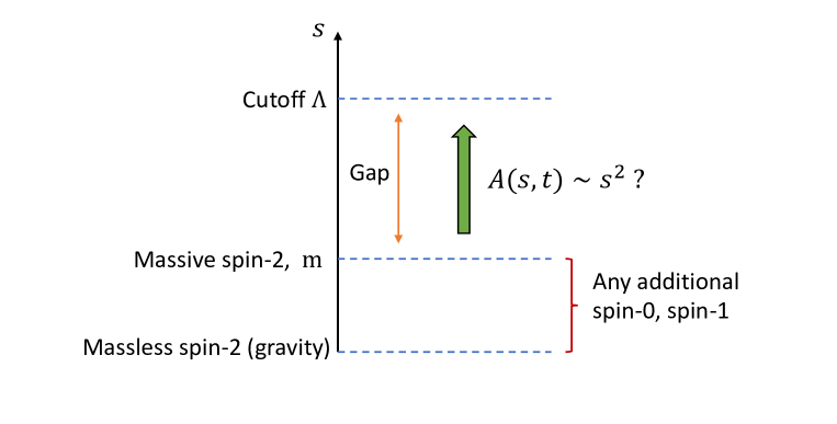
Figure 1: Figure showing the setup of the effective theory that we consider. There is a parametric gap between the mass of the massive spin-2 particle $m$ and the cutoff of the effective theory $\Lambda$. The Regge growth regime we consider is between $m$ and $\Lambda$. As well as gravity, there can be other massive or massless spin-0 or spin-1 particles in the theory, though we demand that their masses are also below the Regge regime. The question we address is whether the amplitude Regge growth can be no faster than $s^{2}$.

The constraint (1) is a version of the Classical Regge Growth conjecture (CRG) proposed in [4]. The original conjecture, as formulated in [4], is the statement that the classical (tree-level) S-matrix of any consistent theory cannot grow faster than $s^{2}$ in the Regge limit, that is for $s\rightarrow\infty$ at fixed $t$. This is not precisely (1), but it certainly inspires it.

The bound (1) is a local bound in the language of [5]. Some strong results on such a bound were developed in [5], for example, showing that it holds in five dimensions or higher for scattering of scalar particles. We refer to [5] for references on the topic, to [6] for a recent review, and to [7, 8, 9, 10] for other recent work.

The theories that we consider, below the cutoff $\Lambda$, are the most general local effective theories with a finite number of derivatives. So we allow for arbitrary higher-derivative operators, but do not account for the possibility of an infinite number of correlated higher derivative operators that can resum into non-analyticities. Such series must correspond to integrating out a particle and are controlled by the mass scale of the particle that has been integrated out. If the particle is spin-0 or spin-1, we include this possibility explicitly by allowing for such states in the effective theory below the cutoff $\Lambda$. If the particle that has been integrated out has spin-2 or higher, then by construction it must have a mass above the cutoff $\Lambda$. Since we are working in the regime $\Lambda\gg\sqrt{s}$, we can reliably neglect such possibilities. In other words, we are interested in theories where one massive spin-2 particle is isolated from other massive spin-2 (or higher) particles, and that includes their effects through an infinite number of correlated higher-derivative operators.

The primary quantity that we are interested in is the growth of the scattering amplitude with $s$. There are many other ways to constrain theories with massive (and massless) spin-2 particles. A small selection of relevant papers follows. Perhaps most similar in nature to our analysis are the papers [14, 15, 16, 17], on which we rely heavily. These papers studied the total energy dependence of scattering amplitudes in the type of theories we are considering. They then used this to bound the cutoff scale through unitarity, or to constrain the spectrum of particles. In particular, in [17] the constraint on the energy growth was shown to lead to a beautiful bound on the spectrum of Kaluza-Klein states in compactifications of higher dimensional pure gravity. There are similar papers which study constraints imposed by superluminality [11, 18, 19]. There are also many papers studying theories of purely massive spin-2 states, so without the massless spin-2 gravity present. We refer to [20, 21] for reviews, and to [22, 23, 24, 25, 26, 27, 28] for some relevant work.

Summary of results

It is simple to summarise our results: we find that there are no possible theories, so any values of the couplings of any operators, which have tree-level scattering that can satisfy the Regge growth bound (1).

As stated, this result holds up to the assumption that there are no relevant infinite correlated series of higher dimension operators, that is, that there is a gap to any poles of further massive spin-2 particles.

We also restrict to four dimensions: $d=4$. This makes the computation more tractable as there are identities which reduce the number of operators. We do not expect our results to change in higher dimensions.

The implications of our results for theories with isolated massive spin-2 particles, coupled to gravity, depend on how strongly one expects the classical Regge growth bound (1) to hold. There is very strong evidence for this, but to the best of our knowledge, it remains to be proven.

1.1 Relation to the Spin-2 conjecture

In this section we discuss some aspects of the spin-2 conjecture proposed in [3]. The conjecture states that in a theory with gravity and a massive spin-2 particle of mass $m$, there is a bound on the cutoff $\Lambda$ of the theory

$$\Lambda\sim\frac{mM_{p}}{M_{w}}\;.$$ (2)

Here $M_{p}$ is the Planck scale and $M_{w}$ is a mass scale which sets the interactions of the massive spin-2 particle. So it is a scale which appears in the coupling of the field, $h_{\mu\nu}$, to the tensor current $T^{\mu\nu}$ which defines its interactions

$$\frac{1}{M_{w}}h_{\mu\nu}T^{\mu\nu}\;.$$ (3)

If $h_{\mu\nu}$ was the graviton, then $M_{w}$ would be $M_{p}$, and $T^{\mu\nu}$ would be the energy-momentum tensor.

The scale $M_{w}$ is somewhat subtle, because the interaction strength may vary for different fields. It is therefore natural to suggest that the cutoff is set by the weakest interaction scale (largest value of $M_{w}$), otherwise the proposal is not well-posed and leads to different cutoffs associated with different fields. A universal interaction which is always present is gravity, and this is always controlled by the mass scale $M_{p}$. This means that if the massive spin-2 field is coupled to gravity we should take $M_{w}\sim M_{p}$. This is then the natural application of the spin-2 conjecture to our setup, which gives the proposed constraint of $\Lambda\sim m$, so that there cannot be a parametric gap from the mass of the spin-2 to an infinite tower of states.

2 Classifying scattering amplitudes

This section aims to present all the ingredients needed to compute the most general $2\rightarrow 2$ tree-level scattering amplitude of a massive spin-2 particle. To do so, we will consider that the massive spin-2 particle can couple to a (massive or massless) scalar particle, a massive spin-1 particle and a massless spin-2 particle. Fermions do not need to be introduced since by momentum conservation they cannot be exchanged between bosons. Massless spin-1 particles can also be ignored, since its coupling with two massive spin-2 particles is not allowed by gauge symmetry.

Tree-level scattering amplitudes can be computed directly, without reference to specific Lagrangian terms, in a model-independent way. One can use the fact that the result has to satisfy Lorentz invariance, crossing symmetry, locality and unitarity to chart all the possible contributions. This can be done using on-shell methods, as explained for instance in [29]. The basic idea behind on-shell amplitudes is that they are invariant under field redefinitions and integration by parts in the Lagrangian, making the classification of the vertices easier. Most of the computations of this part were already developed in [14, 15, 16], in a different context. For that reason, we will only explain the basic steps in the main text, relegating some details to appendices A-D and referring the reader to the aforementioned references for a more detailed discussion.

Let us start by fixing the notation. A particle $i$ has momentum $p_{i}$, spin $l_{i}$ and mass $m_{i}$. We denote its polarisation tensor by $\epsilon_{i}$. This tensor is symmetric, traceless and satisfies $p_{i}^{\mu}\epsilon_{i\mu}=0$. Momentum conservation in our conventions reads $p_{1}+p_{2}+p_{3}=0$. Formally, when constructing the amplitudes, we will write the polarisation matrices as a product of vectors, $\epsilon_{i}=\epsilon_{i\mu\nu}\equiv\epsilon_{i\mu}\epsilon_{i\nu}$, with these vectors satisfying $\epsilon_{i\mu}\epsilon_{i}^{\mu}=0$, $\epsilon_{i\mu}p_{i}^{\mu}=0$. This does not mean that we are assuming the physical polarisations matrices to have rank one: it is only a way in which one can keep track of the contractions more easily. At any point of the computation one can always go back to the $\epsilon_{\mu\nu}$ formalism. In the new language, gauge invariance of the massless spin-1 and spin-2 particles means invariance under $\epsilon_{i\mu}\rightarrow\epsilon_{i\mu}+\alpha p_{i\mu}$, being $\alpha$ an arbitrary constant. We will denote $\epsilon_{i\mu}p_{j}^{\mu}\equiv A_{ij}$, $\epsilon_{i\mu}\epsilon_{j}^{\mu}\equiv B_{ij}=B_{ji}$. All the fields are taken to be canonically normalised, with mass dimension one. Parity-odd interactions always involve contractions with the Levi-Civita tensor $\varepsilon$, $\varepsilon\left(p_{i},p_{j},\epsilon_{k},\epsilon_{l}\right)\equiv\varepsilon^{\mu\nu\alpha\beta}\,p_{i\mu}\,p_{j\nu}\,\epsilon_{k\alpha}\,\epsilon_{l\beta}$. Finally, we denote by $\mathcal{M}_{a,b,c}\left(m_{a},m_{b},m_{c}\right)$ a three-point interaction of particles with spin $a$, $b$, $c$ and masses $m_{a}$, $m_{b}$, $m_{c}$, where the particle $c$ will be the one exchanged.

Two sources of diagrams contribute to any $2\rightarrow 2$ tree-level scattering amplitude: exchange diagrams and contact terms, $\mathcal{A}_{2\rightarrow 2}=A^{\rm contact}+A^{\rm exhcange}$, pictorially represented in figure 2. We discuss them case by case.

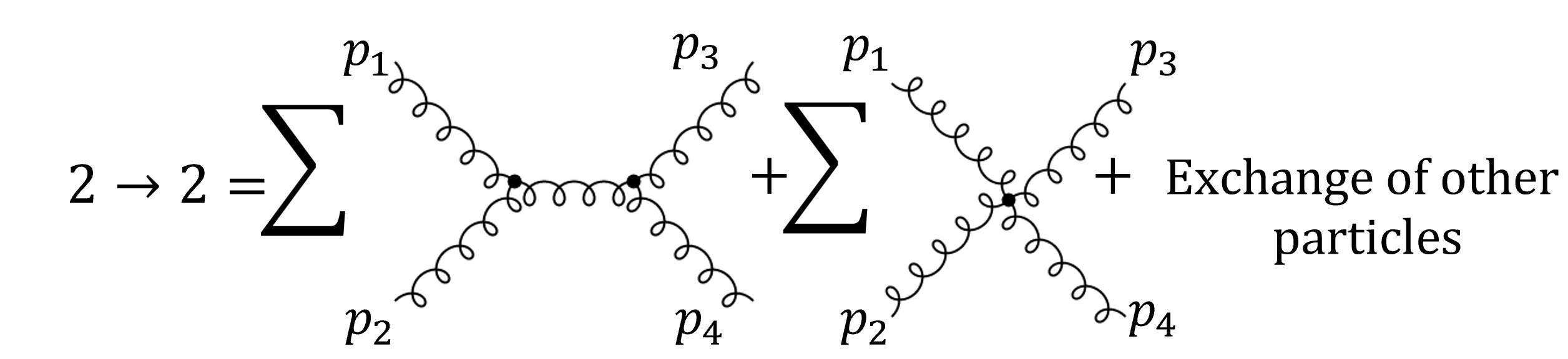
Figure 2: Contributions to the tree-level $2\rightarrow 2$ scattering of any self-interacting particle.

2.1 On shell three-point interactions

The exchange diagrams can be computed in two steps. First, we need to list all the possible on-shell three-point vertices between the two massive spin-2 particles and the exchanged particle. Then, we take two sets of these vertices, and connect them through the corresponding propagator, see figure 3.

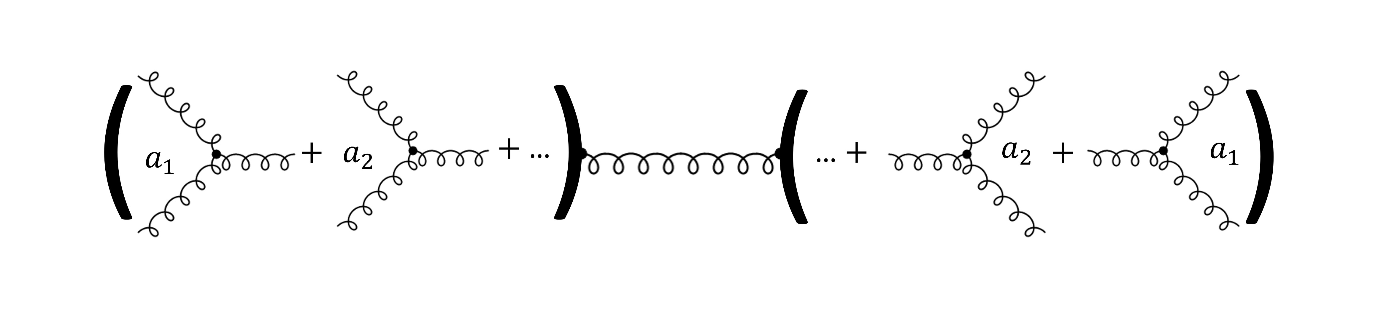
Figure 3: The exchange amplitude can be computed using on-shell three-point vertices. Each vertex is assigned a coefficient $a_{i}$.

This reduces the problem to find all possible on-shell 3-point interactions allowed by Lorentz invariance, crossing symmetry, unitarity, locality and gauge invariance. We discuss how to do this in appendix B, presenting directly the results in the next subsections.

2.1.1 Massive-2, massive-2, massive-2

In this section, we are looking at three-point couplings between three identical massive spin-2 particles of mass $m$. There are in general ten contributions, five of them are parity-even and the other five are parity-odd [30, 14]. One of them (parity-even) comes from a renormalizable piece in the Lagrangian and the rest from non-renormalizable pieces. In four dimensions, $d=4$, this list can be reduced by taking into account that any set of more than four vectors cannot be linearly independent. We discuss these redundancies in appendix B.2, showing directly in table 1 the independent functions.

$\mathcal{M}_{2,2,2}\left(m,m,m\right)$
$\mu B_{12}B_{13}B_{23}\equiv\mathcal{M}_{1}$
$\frac{1}{\Lambda_{2}}\left(B_{13}^{2}A_{21}^{2}+B_{23}^{2}A_{12}^{2}+B_{12}^{2}A_{31}^{2}\right)\equiv\mathcal{M}_{2}$
$\frac{1}{\Lambda_{3}}\left(B_{12}B_{23}A_{12}A_{32}+B_{12}B_{13}A_{21}A_{31}+B_{13}B_{23}A_{12}A_{21}\right)\equiv\mathcal{M}_{3}$
$\frac{1}{\Lambda_{4}^{5}}A_{12}^{2}A_{23}^{2}A_{31}^{2}\equiv\mathcal{M}_{4}$
$\frac{1}{\Lambda_{5}}\left(B_{13}\,B_{23}\,\varepsilon\left(p_{1},p_{2},\epsilon_{1},\epsilon_{2}\right)-B_{12}\,B_{23}\,\varepsilon\left(p_{1},p_{2},\epsilon_{1},\epsilon_{3}\right)+B_{12}\,B_{13}\,\varepsilon\left(p_{1},p_{2},\epsilon_{2},\epsilon_{3}\right)\right)\equiv\mathcal{M}_{5}$
$\frac{1}{\Lambda_{6}^{5}}\left(A_{12}A_{23}A_{31}\left(A_{31}\,\varepsilon\left(p_{1},p_{2},\epsilon_{1},\epsilon_{2}\right)-A_{23}\,\varepsilon\left(p_{1},p_{2},\epsilon_{1},\epsilon_{3}\right)+A_{12}\,\varepsilon\left(p_{1},p_{2},\epsilon_{2},\epsilon_{3}\right)\right)\right)\equiv\mathcal{M}_{6}$

Table 1: Independent three-point amplitudes for three identical massive spin 2-particles with mass $m$ in $d=4$.

Here the spin-2 particle is taken to have mass $m$, and the coefficients $\mu$ and $\Lambda_{i}$ have energy dimension one. Generally, we assume, here and in the next sections, that the scale $\Lambda_{i}$ at which every term becomes relevant can be different. A table with the complete list of the ten contributions is shown in appendix B.2. A Lagrangian basis generating the parity-even elements (the full list, not only the ones presented in table 1) can be found in appendix C.

The total cubic vertex we will be considering for this interaction is therefore (restricting ourselves to four dimensions):

$$\boxed{V_{2,2,2}(m,m,m)\equiv a_{1}\mathcal{M}_{1}+a_{2}\mathcal{M}_{2}+a_{3}\mathcal{M}_{3}+a_{4}\mathcal{M}_{5}+a_{5}\mathcal{M}_{5}+a_{6}\mathcal{M}_{6}}\;.$$ (4)

with $a_{i}$ being arbitrary coefficients.

2.1.2 Massive-2, massive-2, massless-2

In this case we start with six parity-even and nine parity-odd three-point operators at high enough dimension. We can exploit again the fact that we are working in $d=4$ to write some of them as linear combinations of the others. A list with the fifteen interactions is given in appendix B.2, in table 6, whereas below, in table 2, we only write the nine (five even and four odd) linearly independent contributions [19].

$\mathcal{G}_{2,2,2}\left(m,m,0\right)$
$\frac{1}{M_{p}}A_{31}^{2}B_{12}^{2}\equiv\mathcal{G}_{1}$
$\frac{1}{M_{p}}A_{31}B_{12}\left(A_{12}B_{23}+A_{23}B_{13}\right)\equiv\mathcal{G}_{2}$
$\frac{1}{M_{p}}\left(A_{23}B_{13}+A_{12}B_{23}\right){}^{2}\equiv\mathcal{G}_{3}$
$\frac{1}{M_{p}\hat{\Lambda}_{4}^{2}}A_{12}A_{21}A_{31}^{2}B_{12}\equiv\mathcal{G}_{4}$
$\frac{1}{M_{p}\hat{\Lambda}_{5}^{4}}A_{12}^{2}A_{23}^{2}A_{31}^{2}\equiv\mathcal{G}_{5}$
$\frac{1}{M_{p}}\left(B_{23}A_{12}+B_{13}A_{23}\right)\,\varepsilon\left(p_{3},\epsilon_{1},\epsilon_{2},\epsilon_{3}\right)\equiv\mathcal{G}_{6}$
$\frac{1}{M_{p}}B_{12}A_{31}\,\varepsilon\left(p_{3},\epsilon_{1},\epsilon_{2},\epsilon_{3}\right)\equiv\mathcal{G}_{7}$
$\frac{1}{M_{p}\hat{\Lambda}_{8}^{2}}A_{12}A_{23}A_{31}\,\varepsilon\left(p_{3},\epsilon_{1},\epsilon_{2},\epsilon_{3}\right)\equiv\mathcal{G}_{8}$
$\frac{1}{M_{p}\hat{\Lambda}_{9}^{4}}A_{12}A_{23}A_{31}^{2}\,\varepsilon\left(p_{1},p_{2},\epsilon_{1}\,\epsilon_{2}\right)\equiv\mathcal{G}_{9}$

Table 2: Basis of independent three-point amplitudes for two (identical) massive spin-2 particles, one massless spin 2-particle in four dimensions.

The massless spin-2 particle is the graviton, and so each vertex is suppressed with a factor of the Planck mass $M_{p}$. The $\hat{\Lambda}_{i}$ have units of energy and a Lagrangian basis for the parity-even interactions is given in appendix C. The total cubic vertex for this interaction is therefore:

$$\boxed{V_{2,2,2}(m,m,0)\equiv g_{1}\mathcal{G}_{1}+g_{2}\mathcal{G}_{2}+g_{3}\mathcal{G}_{3}+g_{4}\mathcal{G}_{4}+g_{5}\mathcal{G}_{5}+g_{6}\mathcal{G}_{6}+g_{7}\mathcal{G}_{7}+g_{8}\mathcal{G}_{8}+g_{9}\mathcal{G}_{9}}\,.$$ (5)

Here the $g_{i}$ are arbitrary coefficients. Moreover, as discussed in [15, 16] and the references therein, gauge invariance requires

$$2g_{1}=g_{2}\,.$$ (6)

This relation can be derived by studying the Compton scattering of a massive and a massless spin-2 particle, which involves both the massive-2, massive-2, massless-2 and the massless-2, massless-2, massless-2 vertices (the latter coming from the usual graviton self-interaction cubic vertex in the Einstein-Hilbert term).

2.1.3 Massive-2, massive-2, massive-1

Exploiting one more time the fact that we are interested in the case $d=4$, in table 3 we present the (independent) three-point vertices we will be considering, agreeing with [15]. We relegate the full list of interactions for any dimension to appendix B.2, table 7.

$\mathcal{M}_{2,2,1}\left(m,m,m_{1}\right)$
$\left(A_{12}B_{12}B_{23}+A_{21}B_{12}B_{13}\right)\equiv\mathcal{K}_{1}$
$\frac{1}{\tilde{\Lambda}_{2}^{2}}\left(A_{21}A_{12}^{2}B_{23}+A_{21}^{2}A_{12}B_{13}\right)\equiv\mathcal{K}_{2}$
$B_{12}\left(\varepsilon\left(p_{1},\epsilon_{1},\epsilon_{2},\epsilon_{3}\right)-\varepsilon\left(p_{2},\epsilon_{1},\epsilon_{2},\epsilon_{3}\right)\right)\equiv\mathcal{K}_{3}$
$\frac{1}{\tilde{\Lambda}_{4}^{2}}\,\varepsilon\left(p_{1},p_{2},\epsilon_{1},\epsilon_{2}\right)\left(B_{23}A_{12}+B_{13}A_{21}\right)\equiv\mathcal{K}_{4}$

Table 3: Four-dimensional three-point amplitudes for two identical massive spin-2 particles and one massive spin-1 particle

Here $\tilde{\Lambda}_{i}$ is the scale of suppression of the vertex $\mathcal{K}_{i}$ and a parity-even Lagrangian basis is detailed in appendix C. The total cubic vertex for this case is therefore:

$$\boxed{V_{2,2,1}(m,m,m_{1})\equiv k_{1}\mathcal{K}_{1}+k_{2}\mathcal{K}_{2}+k_{3}\mathcal{K}_{3}+k_{4}\mathcal{K}_{4}}\,.$$ (7)

The $k_{i}$ are arbitrary coefficients.

2.1.4 Massive-2, massive-2, scalar

Finally, regarding the coupling with a scalar field $\phi$, our computations match the ones of [16]:

$\mathcal{M}_{2,2,0}\left(m,m,M\right)$
$m_{s}B_{12}^{2}=\mathcal{S}_{1}$
$\frac{1}{\bar{\Lambda}_{2}}A_{12}A_{21}B_{12}=\mathcal{S}_{2}$
$\frac{1}{\bar{\Lambda}_{3}^{3}}A_{12}^{2}A_{21}^{2}=\mathcal{S}_{3}$
$\frac{1}{\bar{\Lambda}_{4}}B_{12}\,\varepsilon\left(p_{1},p_{2},\epsilon_{1},\epsilon_{2}\right)=\mathcal{S}_{4}$
$\frac{1}{\bar{\Lambda}_{5}^{3}}A_{12}A_{23}\,\varepsilon\left(p_{1},p_{2},\epsilon_{1},\epsilon_{2}\right)=\mathcal{S}_{5}$

Table 4: All possible on-shell three-point amplitudes for two massive spin 2-particles and one scalar particle

Here $\bar{\Lambda}_{i}$ suppress the non-renormalizable operators, $m_{s}$ is some interaction scale, the mass $M$ of the scalar can be $M\geq 0$ and a basis of Lagrangian terms for the parity-even amplitudes is derived in appendix C. The total vertex for this interaction is:

$$\boxed{V_{2,2,0}(m,m,M)\equiv s_{1}\mathcal{S}_{1}+s_{2}\mathcal{S}_{2}+s_{3}\mathcal{S}_{3}+s_{4}\mathcal{S}_{4}+s_{5}\mathcal{S}_{5}}\,.$$ (8)

The $s_{i}$ are arbitrary coefficients.

2.2 Exchange amplitude

As explained previously, the contribution of an exchanged particle $k$ to the on-shell $2\rightarrow 2$ scattering of a massive spin-2 particle can be computed as follows. Firstly, we take two sets of vertices $V_{2,2,k}\left(m,m,m_{k}\right)$ defined in equations (4), (5), (7) and (8). Secondly, we “remove” the particle $k$ of the vertices and connect them through the corresponding propagator, given explicitly in appendix A.

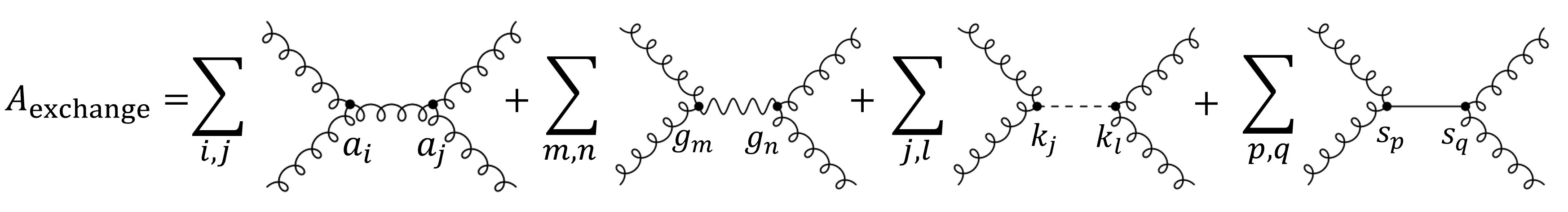
Figure 4: To compute the exchange amplitude we sum over all three-point interactions connected with the correspondent propagator.

We represented this process in figure 4. Before moving to the contact terms, let us pause here for a moment to discuss some details.

Renormalizable and non-renormalizable interactions

In tables 1-4, and in the vertices associated, we treated normalizable and non-renormalizable interactions in the same fashion, implicitly assuming that both contributions can be of the same order. This may look a bit unnatural from a Lagrangian perspective. When dealing with EFTs and higher dimensional operators in $d=4$ we have

$$\mathcal{L}_{\text{EFT}}=\sum\limits_{i}a_{i}\Lambda_{i}^{4-\text{dim}(\mathcal{L}^{i})}\mathcal{L}^{i}_{d\leq 4}+\sum\limits_{j}\frac{b_{j}}{\Lambda_{j}^{\text{dim}\left(\mathcal{L}^{j}\right)-4}}\mathcal{L}^{j}_{d>4}\,,$$ (9)

with $a^{i}$ and $b^{j}$ constants, $\mathcal{L}^{i}_{d\leq 4}$ are the renormalizable and $\mathcal{L}^{j}_{d>4}$ the non-renormalizable terms. Usually, it is natural to expect something like

$$\{a_{i},b_{j}\} \sim\mathcal{O}\left(1\right)\,, \Lambda_{i}^{4-\text{dim}(\mathcal{L}^{i})}\mathcal{L}^{i}_{d\leq 4}\gg\frac{\mathcal{L}^{j}_{d>4}}{\Lambda_{j}^{\text{dim}\left(\mathcal{L}^{j}\right)-4}}\,,$$ (10)

which makes quite unlikely that diagrams coming from non-renormalizable parts in the Lagrangian can cancel the ones coming from renormalizable operators, unless some fine tunning occurs. As a warm-up, when we present our results in section 3 we will begin by studying a scenario like this.

Nevertheless, since we want to be as general as possible, we will also investigate the case in which some $b_{j}$ can be $b_{j}\gg 1$, potentially making the contribution of the non-renormalizable pieces in the Lagrangian of the same order of the renormalizable interactions. This is discussed extensively in section 3.2

Fierz-Pauli coupling

An important role for us is played by the vertex produced when we (minimally) couple the Fierz-Pauli action to gravity. This vertex must be non-vanishing in any theory of a massive spin-2 particle. The Fierz-Pauli Lagrangian, which describes the propagation of a massive spin-2 particle, denoted $h_{\mu\nu}$, in a flat background $\eta_{\mu\nu}$, is

$$\mathcal{L}=-\partial_{\mu}h^{\mu\nu}\partial_{\nu}h+\partial_{\mu}h^{\rho\sigma}\partial_{\rho}h^{\mu}_{\sigma}-\frac{1}{2}\partial_{\mu}h^{\rho\sigma}\partial^{\mu}h_{\rho\sigma}+\frac{1}{2}\partial_{\mu}h\partial^{\mu}h-\frac{1}{2}m^{2}\left(h^{\mu\nu}h_{\mu\nu}-h^{2}\right)\,.$$ (11)

Here $h=\eta^{\mu\nu}h_{\mu\nu}$. Let us now consider a general background with a metric $\tilde{g}_{\mu\nu}$. Lagrangian (11) becomes

$$\mathcal{L}=-\nabla_{\mu}h^{\mu\nu}\nabla_{\nu}h+\nabla_{\mu}h^{\rho\sigma}\nabla_{\rho}h^{\mu}_{\sigma}-\frac{1}{2}\nabla_{\mu}h^{\rho\sigma}\nabla^{\mu}h_{\rho\sigma}+\frac{1}{2}\nabla_{\mu}h\nabla^{\mu}h-\frac{1}{2}m^{2}\left(h^{\mu\nu}h_{\mu\nu}-h^{2}\right)\,,$$ (12)

where the indices are now raised and lowered with the metric $\tilde{g}_{\mu\nu}$ and the derivatives have been replaced by covariant derivatives. To obtain the three-point interactions between two massive and one massless spin-2 particles we expand the metric as

$$\tilde{g}_{\mu\nu} =\eta_{\mu\nu}+\frac{g_{\mu\nu}}{M_{p}}\,, \tilde{g}^{\mu\nu} =\eta^{\mu\nu}-\frac{g^{\mu\nu}}{M_{p}}\,,$$ (13)

and look for the terms of the form $hhg$. There are three different on-shell contributions:

$$h^{\mu\nu}h_{\mu\nu}=\left(\eta^{\alpha\mu}-\frac{g^{\alpha\mu}}{M_{p}}\right)\left(\eta^{\beta\nu}-\frac{g^{\beta\nu}}{M_{p}}\right)h_{\alpha\beta}h_{\mu\nu}|_{hhg}=-\frac{2}{M_{p}}g^{\alpha\mu}\eta^{\beta\nu}h_{\alpha\nu}h_{\mu\beta}=-2\frac{1}{M_{p}}B_{12}B_{13}B_{23}\,,$$ (14)

also

$$\nabla_{\mu}h^{\rho\sigma}\nabla^{\mu}h_{\rho\sigma}|_{hhg}=\tilde{g}^{\mu\nu}\tilde{g}^{\rho\alpha}\tilde{g}^{\sigma\beta}\nabla_{\mu}h_{\rho\sigma}\nabla_{\nu}h_{\alpha\beta}|_{hhg}=-\mathcal{G}_{1}+2\frac{m^{2}}{M_{p}}B_{13}B_{23}B_{12}-2\mathcal{G}_{2}\,,$$ (15)

and in a similar way

$$\nabla_{\mu}h^{\rho\sigma}\nabla_{\rho}h^{\mu}_{\sigma}|_{hhg}=\tilde{g}^{\mu\alpha}\tilde{g}^{\rho\nu}\tilde{g}^{\sigma\beta}\nabla_{\mu}h_{\rho\sigma}\nabla_{\nu}h_{\alpha\beta}|_{hhg}=\frac{1}{2}\mathcal{G}_{3}\,,$$ (16)

with $\mathcal{G}_{3}$ and $\mathcal{G}_{2}$ introduced in section 2.1.2. This means that the Fierz-Pauli contribution to the on-shell three-point vertices can be written as:

$$\mathcal{G}_{FP}|_{hhg}\equiv\frac{1}{2}\left(\mathcal{G}_{3}+\mathcal{G}_{1}+2\mathcal{G}_{2}\right)\,,$$ (17)

which translates into

$$2g_{1}=g_{2}=2g_{3}\neq 0\,.$$ (18)

This non-vanishing combination of three-point couplings must be satisfied in any theory of a massive spin-2 particle coupled to gravity. So in looking for possible consistent theories with appropriate Regge behaviour we are allowed to set any couplings to zero, but must demand that $g_{1}$, $g_{2}$ and $g_{3}$ are non-vanishing and satisfy the constraints (18). Note that this matches the constraint from gauge invariance (6).

Parity symmetry

In the previous sections we introduced parity-even and parity-odd three-point functions, assuming that the theory can be parity violating. Given a particular choice of external polarisations, contributions from even-even and odd-odd vertices will be parity-even, whereas even-odd and odd-even connections will give rise to parity-odd terms.

One can (and we will) avoid this mixing by using the transversity basis for the polarisations, see appendix A, in which the spin of the particles is projected in the transverse direction to the scattering plane. In the transversity basis, the amplitudes $\mathcal{A}$ have definite parity $P$ and they transform under this symmetry as [31]

$$P:\mathcal{A}_{\tau_{1}\tau_{2},\tau_{3}\tau_{4}}\rightarrow(-1)^{\tau_{1}+\tau_{2}-\tau_{3}-\tau_{4}}\mathcal{A}_{\tau_{1}\tau_{2},\tau_{3}\tau_{4}}\,,$$ (19)

where the indices ${}_{\tau_{1}\tau_{2},\tau_{3}\tau_{4}}$ refer to the helicities $\tau_{i}=\{0\,,\,\pm 1\,,\,\pm 2\}$ of the ingoing, 1 and 2, and outgoing, 3 and 4, particles. Regarding the exchange diagrams, this means that when the sum of the helicities of the scattered particles is an even number, only even-even and odd-odd terms contribute; on the contrary, if this sum is an odd number, one must consider even-odd and odd-even interactions. The same reasoning applies to the contact terms: in the transversity basis they decouple according to the parity, as represented in figure 5. For our proposes and to prove our result it will be enough just to study the parity-even amplitudes.

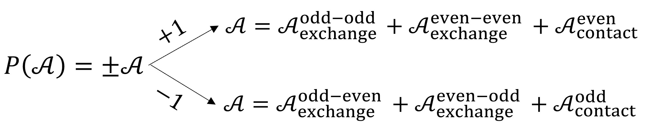
Figure 5: In the transversity basis contributions with different parity decouple.

Let us also comment that we exploit other nice properties of the transversity basis, like the simple form of the crossing symmetry relations. A review of transversity amplitudes and their properties is given in [31, 32, 14].

2.3 Contact terms

Computing all the contact terms is the trickiest and most cumbersome part since, in principle, there is an infinite number of them. To have a situation we can handle, we will only include interactions with an arbitrary but finite number of derivatives, following the algorithm developed in [14, 15, 16]. As discussed in the introduction, neglecting the possibility of an infinite number of correlated higher derivative operators is part of the setting of an isolated massive spin-2 particle that we are studying.

As explained above, we will only need to consider parity-even contact interactions. Parity-even and parity-odd contributions decouple in the transversity basis: when the sum of the helicities of the scattered particles is an even (odd) number only parity-even (parity-odd) terms contribute. To reach our results it is enough to look at the parity-even amplitudes.

We can start with the renormalizable (parity-even) operators. There are only two such operators:

$$B_{13}B_{14}B_{23}B_{24}+B_{12}B_{14}B_{23}B_{34}+B_{12}B_{13}B_{24}B_{34}\,,$$ (20a)

$$B_{14}^{2}B_{23}^{2}+B_{12}^{2}B_{34}^{2}+B_{13}^{2}B_{24}^{2}\,,$$ (20b)

or, written in the Lagrangian basis,

$$h^{1\mu\nu}h^{3\alpha}_{\nu}h^{2\beta}_{\alpha}h^{4}_{\beta\mu}+h^{1\mu\nu}h^{2\alpha}_{\nu}h^{3\beta}_{\alpha}h^{4}_{\beta\mu}+h^{1\mu\nu}h^{2\alpha}_{\nu}h^{4\beta}_{\alpha}h^{3}_{\beta\mu}\,,$$ (21a)

$$h^{1\mu\nu}h^{4}_{\mu\nu}\,h^{2\alpha\beta}h^{3}_{\alpha\beta}+h^{1\mu\nu}h^{2}_{\mu\nu}\,h^{3\alpha\beta}h^{4}_{\alpha\beta}+h^{1\mu\nu}h^{3}_{\mu\nu}\,h^{2\alpha\beta}h^{4}_{\alpha\beta}\,.$$ (21b)

Non-renormalizable contact terms, on the other hand, are many. Schematically, the list of parity-even contact terms with up to $N$ derivatives can be written by first computing

$$V_{2,2,2,2}\left(m,m,m,m\right)=\sum\limits_{n,m,k,l}^{n+k+m+l=N}\sum\limits_{\text{ contractions}}\frac{a_{nmkl}}{\Lambda^{n+m+k+l}}\partial^{n}h\,\partial^{m}h\,\partial^{k}h\,\partial^{l}h\,,$$ (22)

with the first summation taking into account all the possible ways in which the indices of the four $h_{\mu\nu}$ and the derivatives $\partial_{\mu}$ can be contracted, and then symmetrizing under the interchange of any two particles. We are using in (22) the description in terms of fields, instead of $\{A_{ij},B_{mn}\}$, to make the analysis more understandable.

The above discussion serves to illustrate the complexity of the problem. In practice, though, we will follow a slightly different approach, adapting the strategy developed in [14]. In short, one only needs to compute explicitly the tensor structures invariant under the group of permutations that preserve the Mandelstam variables invariant, the so-called kinetic permutations $\Pi^{\text{kin}}$ [33]

$$\Pi^{\text{kin}}=\{\mathds{1},\,(12)(34),\,(13)(24),\,(14)(23)\}\,,$$ (23)

where $(ij)(kl)$ means that we do the permutations $i\leftrightarrow j$ and $k\leftrightarrow l$ at the same time. There are 201 such (parity-even) tensor structures, which we will denote by $\mathds{T}_{a}$ and that we list in appendix E. Then, each of these structures is multiplied by an arbitrary polynomial $f_{a}\left(s,t\right)$ of $s$ and $t$, yielding:

$$\boxed{\tilde{A}^{\text{contact}}=\sum\limits_{a}^{201}f_{a}\left(s,t\right)\mathds{T}_{a}}\,.$$ (24)

We are calling this intermediate result $\tilde{A}^{\text{contact}}$ to distinguish it from the actual $A^{\text{contact}}$, invariant under the permutation of any two particles. Indeed, to obtain $A^{\text{contact}}$, one has to impose the remaining permutation symmetries in $\tilde{A}^{\text{contact}}$. These other permutations, under which $(s,t,u)$ are not invariant, will lead to crossing relations that must be satisfied. In section 3.2 we will explain extensively what are these crossing constraints and how to obtain $A^{\text{contact}}$.

3 Constraining theories through Regge growth

We consider the most general effective theory of a massive spin-2 particle and impose the constraint (1). The result we are after is whether such a theory, satisfying (1), exists. At least, it must contain the couplings (17) as non-vanishing, and so satisfy (18). That is the starting point. The rest of the couplings are allowed to take any values, including vanishing. The analysis follows a simple procedure:

1. Compute all exchange and contact contributions for all polarisations. This results in some function of $s$ and $t$

   $$\mathcal{A}_{2\rightarrow 2}=\sum\limits_{i}\mathcal{A}_{i}^{\text{exchange}}+\sum\limits_{j}\mathcal{A}_{j}^{\text{contact}}\equiv\mathcal{A}\left(s,t\right)\,.$$ (25)

2. Take the limit $\{s\gg|t|,m^{2}\}$. Expand $\mathcal{A}\left(s,t\right)$ in powers of $s$

   $$\lim_{s\gg t,m^{2}}\mathcal{A}\left(s,t\right)=\dots+\mathcal{A}_{2}\left(t\right)s^{2}+\mathcal{A}_{3}\left(t\right)s^{3}+\dots\mathcal{A}_{n}\left(t\right)s^{n}\,.$$ (26)

3. Impose

   $$\mathcal{A}_{m}\left(t\right) =0\,,\,\,\text{for }\,\,m\geq 3\,,\,\,\forall\,t<\,0\,,$$ (27)

   and for any external polarisation configuration. Equation (27) will yield several sub-equations, one for each power of $t^{i}$. These sub-equations will depend linearly on the coefficients of the contact terms and quadratically on the three-point couplings.

4. Solve the previous equations. If (1) can be satisfied non-trivially, some relation between the three-point and the four-point couplings will be obtained. Otherwise, no possible theory satisfying (1) exists.

3.1 A maximally natural scenario

As a warm-up, we will start by considering a simplified scenario in which all dimensionless couplings are taken to be of order one. So this means that the magnitude of operators is controlled by their dimension and the cutoff scale $\Lambda$. So this is a type of maximally natural scenario.

The starting point is the demand that the combination of terms in (17) is non-vanishing. These operators have all mass dimension five. By direct computation, it is easy to check that with only these three pieces, the four-point scattering of a massive spin-2 particle can never satisfy (1).

We therefore need to see if the other operators can be chosen to cancel the too-fast Regge growth. The “maximally natural” scenario we are considering means that such a possible cancellation is very restricted. Regarding the contact terms, only the ones with mass dimension less than or equal to six can be useful. Higher dimensional operators will be suppressed by higher powers of $\Lambda$, which makes them parametrically smaller. We would have equations like

$$a\frac{s^{3}}{\Lambda^{2}m^{4}}+b\frac{s^{3}}{\Lambda^{4}m^{2}}+c\frac{s^{3}}{\Lambda^{6}}+\dots=0\,,$$ (28)

which, unless the coupling constants satisfy $c\gg b\gg a$, as we are forbidding in this section, must be solved order by order. For the same reasons, we can ignore three-point vertices suppressed by $\Lambda^{n}$ for $n\geq 2$.

This leaves us with the following three-point vertices:

$$V_{2,2,2}\left(m,m,m\right)=a_{1}\mathcal{M}_{1}+a_{2}\mathcal{M}_{2}+a_{3}\mathcal{M}_{3}+a_{5}\mathcal{M}_{5}\,,$$ (29a)

$$V_{2,2,2}\left(m,m,0\right)=g_{1}\mathcal{G}_{1}+g_{2}\mathcal{G}_{2}+g_{3}\mathcal{G}_{3}+g_{6}\mathcal{G}_{6}+g_{7}\mathcal{G}_{7}\,,$$ (29b)

$$V_{2,2,1}\left(m,m,m_{1}\right)=k_{1}\mathcal{K}_{1}+k_{3}\mathcal{K}_{3}\,,$$ (29c)

$$V_{2,2,0}\left(m,m,M\right)=s_{1}\mathcal{S}_{1}+s_{2}\mathcal{S}_{2}+s_{4}\mathcal{S}_{4}\,.$$ (29d)

Four-point interactions with up to two derivatives have to be included. Focusing only on the parity-even terms, there are 12 distinct choices:

• 2 contact terms with no derivatives, already discussed in (20). We multiply them by $\{c_{1},\,c_{2}\}$ .

• 4 contact terms with two derivatives with the indices of the derivatives contracted among themselves (terms of the form $\partial^{\mu}h\partial_{\mu}hhh\,+\,\text{symmetrization}$). They come with the couplings $\{c_{3},\,\dots\,,c_{6}\}$ .

• 6 contact terms with two derivatives with the indices of the derivatives contracted with the massive spin-2 fields (terms of the form $\partial^{\mu}\partial^{\nu}h_{\mu\nu}hhh\,+\,\text{symmetrization}$). We use $\{c_{7},\,\dots\,,c_{12}\}$ to parameterize these interactions.

Overall, there are $12+14$ degrees of freedom. We will show now that this system can never satisfy (1), writing some intermediate steps. We will indicate by $ij\rightarrow ab$ the helicity of the particles scattered, so taking values $\{0,\,\pm 1,\,\pm 2\}$.

• From $11\rightarrow 11$ at order $s^{4}t$:

  $$\frac{a_{2}^{2}}{m^{8}M_{p}^{2}}=0\,\,\longrightarrow\,\,a_{2}=0\,.$$ (30)

• From $00\rightarrow 00$ at order $s^{6}t$ (using $a_{2}=0$):

  $$\frac{a_{3}^{2}}{m^{12}M_{p}^{2}}=0\,\,\longrightarrow\,\,a_{3}=0\,.$$ (31)

• From $(-1)(2)\rightarrow(-1)(-2)$ at order $s^{3}\sqrt{t}$ (using $a_{2}=0=a_{3}$):

  $$\frac{a_{5}^{2}+3\left(4(g_{2}-2g_{3})^{2}+(g_{7}-2g_{6})^{2}\right)}{m^{5}\text{Mp}^{2}}=0\,\,\longrightarrow\,\,a_{5}=0\,,\,g_{2}=2g_{3}\,,\,g_{7}=2g_{6}$$ (32)

• From the equations involving just contact couplings

  $$\{c_{7},\,\dots\,,c_{12}\}=0\,.$$ (33)

• Plugging these constraints in the other equations the only real solution is:

  $$\{a_{1},a_{5},g_{1},g_{3},g_{5},g_{6},s_{2},k_{1},k_{3}\}=0\,,$$ (34)

  with $s_{1}$ being a free parameter.

This means that all cubic couplings, except for the renormalizable interaction with the scalar field, must vanish. In particular, the required combination (17) also, and so the theory is trivial. In other words, under the assumptions made, there cannot exist a theory of a massive spin-2 particle consistent with (1).

3.2 The general case

After discussing a simplified version of the problem, we will now tackle the general case, in which all exchange and contact diagrams with any finite number of derivatives are included with arbitrary coefficients. Our strategy follows closely, though not identically, the one developed in [14, 15, 16].

In what follows, we will describe in detail the procedure without showing any explicit computation. The reader interested can find an ancillary Mathematica file attached to the paper with the code used. We only focus on the parity-even choices of polarisations, recall equation (19), since this is enough to arrive at our results.

To start with, let us split the four-point scattering amplitude $A_{\tau_{1}\tau_{2},\tau_{3}\tau_{4}}$ into the contact and the exchange contributions:

$$A_{\tau_{1}\tau_{2},\tau_{3}\tau_{4}}=A^{\text{exchange}}_{\tau_{1}\tau_{2},\tau_{3}\tau_{4}}+A^{\text{contact}}_{\tau_{1}\tau_{2},\tau_{3}\tau_{4}}\,,$$ (35)

where again the indices ${}_{\tau_{1}\tau_{2},\tau_{3}\tau_{4}}$ refer to the helicities $\tau_{i}=\{0\,,\,\pm 1\,,\,\pm 2\}$ of the ingoing, 1 and 2, and outgoing, 3 and 4, particles. Then, the steps to follow are:

• Compute $A^{\text{exchange}}_{\tau_{1}\tau_{2},\tau_{3}\tau_{4}}$. As commented in in section 2.1 one needs to take two sets of the three-point vertices,

  $$V_{2,2,2}\left(m,m,m\right)=a_{1}\mathcal{M}_{1}+a_{2}\mathcal{M}_{2}+a_{3}\mathcal{M}_{3}+a_{4}\mathcal{M}_{4}+a_{5}\mathcal{M}_{5}+a_{6}\mathcal{M}_{6}\,,$$ (36a)

  $$V_{2,2,2}\left(m,m,0\right)=g_{1}\mathcal{G}_{1}+g_{2}\mathcal{G}_{2}+g_{3}\mathcal{G}_{3}+g_{4}\mathcal{G}_{4}+g_{5}\mathcal{G}_{5}+g_{6}\mathcal{G}_{6}+g_{7}\mathcal{G}_{7}$$

  $$+g_{8}\mathcal{G}_{8}+g_{9}\mathcal{G}_{9}\,,$$ (36b)

  $$V_{2,2,1}\left(m,m,m_{1}\right)=k_{1}\mathcal{K}_{1}+k_{2}\mathcal{K}_{2}+k_{3}\mathcal{K}_{3}+k_{4}\mathcal{K}_{4}\,,$$ (36c)

  $$V_{2,2,0}\left(m,m,M\right)=s_{1}\mathcal{S}_{1}+s_{2}\mathcal{S}_{2}+s_{3}\mathcal{S}_{3}+s_{4}\mathcal{S}_{4}+s_{5}\mathcal{S}_{5}\,,$$ (36d)

  “remove” the exchanged particle and connect them through the correspondent propagator. We listed the functions and conventions we used in appendix A. The result of this step is an amplitude that depends on the product of the twenty-four three-point coupling constants.

• Take an ansatz for $A^{\text{contact}}_{\tau_{1}\tau_{2},\tau_{3}\tau_{4}}$ with the kinematical singularities [32, 34, 35] factored out

  $$A^{\text{contact}}_{\tau_{1}\tau_{2},\tau_{3}\tau_{4}}\left(s,t\right)=\frac{a^{\text{contact}}_{\tau_{1}\tau_{2},\tau_{3}\tau_{4}}\left(s,t\right)+i\sqrt{stu}\,b^{\text{contact}}_{\tau_{1}\tau_{2},\tau_{3}\tau_{4}}\left(s,t\right)}{\left(s-4m^{2}\right)^{|\sum\limits_{i}\tau_{i}|/2}}\,,$$ (37)

  with $a^{\text{contact}}_{\tau_{1}\tau_{2},\tau_{3}\tau_{4}}=\sum\limits_{n,m}\,\alpha^{\tau_{1}\tau_{2},\tau_{3}\tau_{4}}_{m,n}\,t^{m}\,s^{n}$ and $b^{\text{contact}}_{\tau_{1}\tau_{2},\tau_{3}\tau_{4}}=\sum\limits_{i,j}\,\beta^{\tau_{1}\tau_{2},\tau_{3}\tau_{4}}_{i,j}\,t^{i}\,s^{j}$ arbitrary polynomials at this point. The indices $\{n,m\}$ and $\{i,k\}$ run from 0 to $n+m=p$ and $i+j=k$, with $p$ and $k$ such that in the Regge limit, $\{s\gg|t|\,\}$, the real and imaginary parts of both $A^{\text{exchange}}$ and $A^{\text{contact}}$ have the same energy scaling. The particular form of the ansatz follows from the fact that we are using the transversity basis for the polarisations, a basis which we introduced in section 2.2.

• Constrain $a^{\text{contact}}_{\tau_{1}\tau_{2},\tau_{3}\tau_{4}}$ and $b^{\text{contact}}_{\tau_{1}\tau_{2},\tau_{3}\tau_{4}}$ by requiring that, in the Regge limit, the total amplitude $A_{\tau_{1}\tau_{2},\tau_{3}\tau_{4}}$ does not grow faster than $s^{2}$. In practice this means:

  $$\lim_{s\to\infty\,,\,\forall t<0}\left[\frac{A^{\text{exchange}}_{\tau_{1}\tau_{2},\tau_{3}\tau_{4}}}{s^{3}}+\frac{A^{\text{contact}}_{\tau_{1}\tau_{2},\tau_{3}\tau_{4}}}{s^{3}}\right]=0\,.$$ (38)

  which gives a series of relations between the contact couplings $\{\alpha^{\tau_{1}\tau_{2},\tau_{3}\tau_{4}}_{m,n},\,\beta^{\tau_{1}\tau_{2},\tau_{3}\tau_{4}}_{m,n}\}$ and the product of cubic couplings $\{a_{i},g_{j},k_{m},s_{n}\}$. By rewriting these products as new variables

  $$a_{i}a_{j}\equiv a_{ij}\,,\,g_{i}g_{j}\equiv g_{ij}\,,\,k_{i}k_{j}\equiv k_{ij}\,,\,s_{i}s_{j}\equiv s_{ij}\,,$$ (39)

  one can linearise the equations resulting from (38), making the problem computationally more tractable. The condition (38) is different from the one imposed in [14, 15, 16], who were interested in the case $\lim_{\{s\to\infty\,,\,-t\to\infty\}}\frac{A_{\tau_{1}\tau_{2},\tau_{3}\tau_{4}}}{s^{3}}=0$ with $s/t$ fixed.

• At this stage we need to impose further restrictions on the contact interactions which come from crossing symmetries. Imposing the crossing symmetries on the contact terms requires[31, 36]

  $$\mathcal{A}^{\rm contact}_{\tau_{1}\tau_{2},\tau_{3}\tau_{4}}(s,t) =e^{i\left(\pi-\chi_{t}\right)\sum_{j}\tau_{j}}\mathcal{A}^{\rm contact}_{-\tau_{1}-\tau_{3},-\tau_{2}-\tau_{4}}(t,s),$$ (40a)

  $$\mathcal{A}^{\rm contact}_{\tau_{1}\tau_{2},\tau_{3}\tau_{4}}(s,t) =e^{i\left(\pi-\chi_{u}\right)\sum_{j}\tau_{j}}\mathcal{A}^{\rm contact}_{-\tau_{1}-\tau_{4},-\tau_{3}-\tau_{2}}(u,t),$$ (40b)

  where

  $$e^{-i\chi_{t}}\equiv\frac{-st-2im\sqrt{stu}}{\sqrt{s(s-4m^{2})t(t-4m^{2})}},\quad e^{-i\chi_{u}}\equiv\frac{-su+2im\sqrt{stu}}{\sqrt{s(s-4m^{2})u(u-4m^{2})}}.$$ (41)

  These equations relate some of the surviving $\{\alpha^{\tau_{1}\tau_{2},\tau_{3}\tau_{4}}_{m,n},\,\beta^{\tau_{1}\tau_{2},\tau_{3}\tau_{4}}_{m,n}\}$ to the constants $\{c_{ij},\,g_{ij},\,k_{ij},\,s_{ij}\}$. As explained some steps before, this elegant form of the crossing symmetries (40) is a feature of the transversity basis.

• Make the ansatz for $\mathcal{A}^{\rm contact}$ consistent with the expression (24). This should hold for all polarisations, so that

  $$\mathcal{A}^{\rm contact}_{\tau_{1}\tau_{2},\tau_{3}\tau_{4}}=\sum\limits_{a}^{201}f_{a}^{\tau_{1}\tau_{2},\tau_{3}\tau_{4}}\left(s,t\right)\mathds{T}_{a}^{\tau_{1}\tau_{2},\tau_{3}\tau_{4}}\;,$$ (42)

  for all

  $$\tau_{1}+\tau_{2}-\tau_{3}-\tau_{4}=k\,,\;\;\;\;\;\,k\in 2\mathds{Z}\;.$$ (43)

  To do this, omitting for clearness the polarisation indices, one needs to expand the polynomial $f_{a}\left(s,t\right)=\sum\limits_{ij}f_{ij}t^{i}s^{j}$ and match it at each order with the result obtained in the previous step. Finally, one has to undo the change of variable in the product of cubic couplings and make sure that everything is consistent: there cannot be contradictions, e.g. $c_{ii}=0,\,c_{ij}\neq 0$, and all couplings must be real. After this step, we end up with the most general $2\rightarrow 2$ scattering of a massive spin-2 particle compatible with the Regge growth requirement (1).

After implementing this 5-step procedure, we find that the Regge growth bound (1) can only be satisfied if:

$$a_{i}=0\,,\,\forall i\,; g_{j}=0\,,\,\forall j\geq 2\,; k_{l}=0\,,\,\forall l\,; s_{n}=0\,,\,\forall n\geq 2\,.$$ (44)

Combining this result with the fact that interactions with gravity must include the Fierz-Pauli action, see equation (18), we arrive at

$$\boxed{a_{i}=0\,,\,\forall i}\, \boxed{g_{j}=0\,,\,\forall j} \boxed{k_{l}=0\,,\,\forall l}\, \boxed{s_{n}=0\,,\,\forall n\geq 2}\,\;.$$ (45)

So all Lagrangian terms must vanish (with the sole exception of the scalar coupling $h^{\mu\nu}h_{\mu\nu}\phi$). Hence, there is no such theory. We therefore arrive at the main result of this paper: theories containing a single massive spin-2 particle are not compatible with (1). Recall that this follows under the following assumptions:

• The massive spin-2 particle is allowed to couple to a massless spin-2, a massive spin-1 and a massive or massless scalar particle.

• All contact terms with any finite number of derivatives are taken into account, but infinite series of contact terms which can re-sum to poles are not included.

4 Summary

As discussed in the introduction, it is simple to summarise our results: we find that there are no possible theories with a massive spin-2 particle coupled to gravity, and a gap to the next spin-2 (or higher) states, which satisfy the constraint (1). So a theory of an isolated massive spin-2 particle, coupled to gravity, will necessarily exhibit Regge growth which is faster than $s^{2}$ in the gap between the massive spin-2 particle and any further spin-2 (or higher) states.

This result holds up to the assumption of neglecting infinite series of higher derivative terms which can resum into a pole. As explained, this is justified because such a series would only be relevant near the mass scale of the spin-2 (or higher) particle which was integrated out to generate it, and we assume a gap to any such scales.

Our results strongly suggest that theories of isolated massive spin-2 particles, coupled to gravity, are in the Swampland. To prove this one would need to prove that the fast Regge scaling (1) is inconsistent. This is essentially what the Classical Regge Growth Conjecture proposes [4]. As well as what is expected from general Regge growth bounds, for example as studied in [5].

Of course, theories with massive spin-2 states do occur in ultraviolet complete consistent theories, but they are always part of an infinite tower. In restricted settings, for example when pure gravity is dimensionally reduced, it is possible to bound the gap between massive spin-2 states [17]. We expect that such a bound can be deduced even for the most general possible theories, as studied in this paper. We leave a proof of this for future work.

Finally, let us note that theories where there is no massless spin-2 state, but only an isolated massive spin-2 one, so theories of massive gravity, also exhibit the fast Regge growth we have found. This follows from our results, which are that the only couplings (so non-quadratic) interactions which are compatible with slow Regge growth are the coupling to a scalar field.

Acknowledgments

We would like to thank James Bonifacio and Kurt Hinterbichler for very helpful discussions and explanations and Shiraz Minwalla for useful discussions. The work of EP and JQ is supported by the Israel Science Foundation (grant No. 741/20). The work of EP is supported by the Israel planning and budgeting committee grant for supporting theoretical high energy physics. The work of SK, EP and JQ is supported by the German Research Foundation through a German-Israeli Project Cooperation (DIP) grant “Holography and the Swampland”. The work of SK is also supported in part by an ISF, centre for excellence grant (grant number 2289/18), Simons Foundation grant 994296, and Koshland Fellowship.

Appendix A Kinematics and convention

In this appendix we will write explicitly the definitions of the kinematical variables used to compute the $2\rightarrow 2$ scattering of the massive spin-2 particle. We will use the conventions of [14, 15, 16].

The incoming particles are labelled by $1$ and $2$, and outgoing particles by $3$ and $4$. Momentum conservation requires

$$p_{1}+p_{2}=p_{3}+p_{4}\,,$$ (46)

where we take

$$p_{i}^{\mu}=\left(E,p\sin\theta_{j},0,p\cos\theta_{j}\right)\,,$$ (47)

with $E^{2}=p^{2}+m^{2}$ and $\theta_{1}=0$, $\theta_{2}=\pi$, $\theta_{3}=\theta$, $\theta_{4}=\theta-\pi$. The Mandelstam variables are

$$s= -\left(p_{1}+p_{2}\right)^{2}\,, t =-\left(p_{1}-p_{3}\right)^{2}\,, u =-\left(p_{1}-p_{4}\right)^{2}\,,$$ (48)

and we are taking the metric $\eta=\text{diag}\left(-1,1,1,1\right)$. They satisfy

$$s+t+u=4m^{2}\,,$$ (49)

with $m$ the mass of the spin-2 particle, and are related to $E$ and $\theta$ by

$$s =4E^{2}\,, cos\theta=1-\frac{2t}{4m^{2}-s}\,.$$ (50)

For the three polarisation vectors of the massive spin-1 particles we use the so-called transversity basis [31, 36, 32] in which the spin of the particles are projected on the axis orthogonal to the scattering plane

$$\epsilon^{\mu}_{\left(\pm 1\right)}\left(p_{j}\right) =\frac{i}{\sqrt{2}m}\left(p,E\sin\theta_{j}\pm im\cos\theta_{j},0,E\cos\theta_{j}\mp im\sin\theta_{j}\right)\,,$$ (51a)

$$\epsilon^{\mu}_{\left(0\right)}\left(p_{j}\right) =\frac{1}{m}\left(0,0,1,0\right)\,.$$ (51b)

They are transverse and orthonormal. From them one can construct the five polarisation tensors of massive spin-2 particles

$$\epsilon^{\mu\nu}_{\left(\pm 2\right)} =\epsilon^{\mu}_{\left(\pm 1\right)}\epsilon^{\nu}_{\left(\pm 1\right)}\,,$$ (52a)

$$\epsilon^{\mu\nu}_{\left(\pm 1\right)} =\frac{1}{\sqrt{2}}\left(\epsilon^{\mu}_{\left(\pm 1\right)}\epsilon^{\nu}_{\left(0\right)}+\epsilon^{\mu}_{\left(0\right)}\epsilon^{\nu}_{\left(\pm 1\right)}\right)\,,$$ (52b)

$$\epsilon^{\mu\nu}_{\left(0\right)} =\frac{1}{\sqrt{6}}\left(\epsilon^{\mu}_{\left(1\right)}\epsilon^{\nu}_{\left(-1\right)}+\epsilon^{\mu}_{\left(-1\right)}\epsilon^{\nu}_{\left(1\right)}+2\epsilon^{\mu}_{\left(0\right)}\epsilon^{\nu}_{\left(0\right)}\right)\,,$$ (52c)

which are transverse, traceless and orthonormal.

Regarding the propagators, the propagator of a scalar particle with mass $M$ is

$$\frac{-i}{p^{2}+M^{2}-i\epsilon}\,.$$ (53)

For a massive spin-1 particle, first we need to introduce the projector

$$\Pi_{\mu\nu}\left(\tilde{m}\right)=\eta_{\mu\nu}+\frac{p_{\mu}p_{\nu}}{\tilde{m}^{2}}\,,$$ (54)

from which one can write the propagator of a massive spin-1 particle with mass $m_{1}$ as

$$P_{\mu\nu}=\frac{-i\Pi_{\mu\nu}\left(m_{1}\right)}{p^{2}+m_{1}^{2}-i\epsilon}\,.$$ (55)

Finally, the propagator of a massive spin-2 particle of mass $m$ is

$$P_{\mu_{1}\mu_{2},\nu_{1}\nu_{2}}=\frac{-i}{2}\frac{\Pi_{\mu_{1}\nu_{1}}\Pi_{\mu_{2}\nu_{2}}+\Pi_{\mu_{1}\nu_{2}}\Pi_{\mu_{2}\nu_{1}}-\frac{2}{3}\Pi_{\mu_{1}\mu_{2}}\Pi_{\nu_{1}\nu_{2}}}{p^{2}+m^{2}-i\epsilon}\,,$$ (56)

with $\Pi_{\nu_{1}\nu_{2}}=\Pi_{\nu_{1}\nu_{2}}\left(m\right)$, whereas for a massless spin-2 (in de Donder gauge) it reads

$$\tilde{P}_{\mu_{1}\mu_{2},\nu_{1}\nu_{2}}=\frac{-i}{2}\frac{\eta_{\mu_{1}\nu_{1}}\eta_{\mu_{2}\nu_{2}}+\eta_{\mu_{1}\nu_{2}}\eta_{\mu_{2}\nu_{1}}-\eta_{\mu_{1}\mu_{2}}\eta_{\nu_{1}\nu_{2}}}{p^{2}-i\epsilon}\,.$$ (57)

Appendix B On-shell quantities

In the first part of this appendix we explain how to construct the on-shell three-point vertices presented in section 2.1, following the procedure developed in [29]. In the second part of the appendix B.2 we list all possible vertices.

B.1 General discussion

Let us start by fixing the notation. We are interested in the on-shell three-point interactions of 3 particles with masses $m_{i}$, momenta $p_{i}$, spin $s_{i}$ and polarisation tensors $\epsilon_{i}$, with $i=1,2,3$ respectively. They satisfy $\epsilon_{i}\cdot p_{i}=0$, whereas the fact that they are on shell means $p_{i}^{2}=p_{i}\cdot p_{i}=-m_{i}^{2}$. Our convention for momentum conservation reads $\sum\limits_{i}p_{i}=0$. As explained at the beginning of section 2 we will formally write the polarisation matrices as the product of vectors $\epsilon_{i\mu\nu}=\epsilon_{i\mu}\epsilon_{i\nu}$, as a trick to keep track of the contractions more easily.

Parity even

The parity-even on-shell three-point vertices are polynomial functions of the product of $\{\epsilon_{i\mu},p_{j}\}$, homogeneous of order $s_{a}$ in each $\epsilon_{i\mu}$ -from now on, and making abuse of notation, we will call for simplicity $\epsilon_{i\mu}\equiv\epsilon_{i}$-. Taking into account that $\epsilon_{i}\cdot\epsilon_{i}=0=\epsilon_{i}\cdot p_{i}$ these interactions can be constructed from nine contractions

$$\epsilon_{1} \cdot\epsilon_{2}\,, \epsilon_{1} \cdot\epsilon_{3}\,, \epsilon_{2} \cdot\epsilon_{3}\,,$$

$$\epsilon_{1} \cdot p_{2}\,, \epsilon_{1} \cdot p_{3}\,, \epsilon_{2} \cdot p_{1}\,,$$ (58)

$$\epsilon_{2} \cdot p_{3}\,, \epsilon_{3} \cdot p_{1}\,, \epsilon_{3} \cdot p_{2}\,,$$

which, using $p_{1}+p_{2}+p_{3}=0$, can be reduced further to

$$\epsilon_{1}\cdot\epsilon_{2}\,, \epsilon_{1}\cdot\epsilon_{3}\,, \epsilon_{2}\cdot\epsilon_{3}\,,$$

$$\epsilon_{1}\cdot p_{2}\,, \epsilon_{3}\cdot p_{1}\,, \epsilon_{2}\cdot p_{1}\,,$$ (59)

$$\cancelto{-\epsilon_{1}\cdot p_{2}}{\epsilon_{1}\cdot p_{3}}\,, \cancelto{-\epsilon_{3}\cdot p_{1}}{\epsilon_{3}\cdot p_{2}}\,, \cancelto{-\epsilon_{2}\cdot p_{1}}{\epsilon_{2}\cdot p_{3}}\,,$$

and so the most general parity-even three-point interaction must take the form

$$\mathcal{M}_{s_{1},s_{2},s_{3}}\left(p_{1},p_{2},p_{3}\right)=C\left(\epsilon_{1}\cdot\epsilon_{2}\right)^{x_{12}}\left(\epsilon_{1}\cdot\epsilon_{3}\right)^{x_{13}}\left(\epsilon_{2}\cdot\epsilon_{3}\right)^{x_{23}}\left(\epsilon_{1}\cdot p_{2}\right)^{y_{12}}\left(\epsilon_{3}\cdot p_{1}\right)^{y_{31}}\left(\epsilon_{2}\cdot p_{1}\right)^{y_{21}}\,,$$ (60)

where $C$ is an arbitrary constant and the exponents are non-negative integers that have to satisfy

$$x_{12}+x_{13}+y_{12} =s_{1}\,,$$ (61a)

$$x_{12}+x_{23}+y_{21} =s_{2}\,,$$ (61b)

$$x_{13}+x_{23}+y_{31} =s_{3}\,,$$ (61c)

$$s_{i}\geq 0\,.$$ (61d)

In the particular case $d=4$, we can also use the fact that the Gram determinant of the vectors $\{\epsilon_{1},\epsilon_{2},\epsilon_{3},p_{1},p_{2}\}$ must vanish: five vectors cannot be all independent in four dimensions. We already exploded this fact in the main text.

Parity odd

On the other hand, parity-odd three-point functions are constructed from contractions with the Levi-Civita tensor $\varepsilon$, $\varepsilon\left(p_{i},p_{j},\epsilon_{k},\epsilon_{l}\right)\equiv\varepsilon_{\mu\nu\alpha\beta}\,p^{i\mu}\,p^{j\nu}\,\epsilon^{k\alpha}\,\epsilon^{l\beta}\,$ or $\varepsilon\left(p_{i},\epsilon_{j},\epsilon_{k},\epsilon_{l}\right)\equiv\varepsilon_{\mu\nu\alpha\beta}\,\epsilon^{i\mu}\,\epsilon^{j\nu}\,\epsilon^{k\alpha}\,\epsilon^{l\beta}$, plus some extra parity-even structures to include enough number of $\epsilon_{i}$. The most general parity-odd on-shell three-point amplitude can always be written as:

$$\mathcal{M}_{s_{1},s_{2},s_{3}}\left(p_{1},p_{2},p_{3}\right)=$$

$$D\varepsilon\left(p_{1}^{z_{1}},p_{2}^{z_{2}},\epsilon_{1}^{z_{3}},\epsilon_{2}^{z_{4}},\epsilon_{3}^{z_{5}},\right)\left(\epsilon_{1}\cdot\epsilon_{2}\right)^{\tilde{x}_{12}}\left(\epsilon_{1}\cdot\epsilon_{3}\right)^{\tilde{x}_{13}}\left(\epsilon_{2}\cdot\epsilon_{3}\right)^{\tilde{x}_{23}}\left(\epsilon_{1}\cdot p_{2}\right)^{\tilde{y}_{12}}\left(\epsilon_{3}\cdot p_{1}\right)^{\tilde{y}_{31}}\left(\epsilon_{2}\cdot p_{1}\right)^{\tilde{y}_{21}}\,,$$ (62)

where $D$ is an arbitrary constant and the exponents, non-negative integers, have to satisfy

$$\tilde{x}_{12}+\tilde{x}_{13}+\tilde{y}_{12}+z_{3} =s_{1}\,,$$ (63a)

$$\tilde{x}_{12}+\tilde{x}_{23}+\tilde{y}_{21}+z_{4} =s_{2}\,,$$ (63b)

$$\tilde{x}_{13}+\tilde{x}_{23}+\tilde{y}_{31}+z_{5} =s_{3}\,,$$ (63c)

$$z_{1}+z_{2}+z_{3}+z_{4}+z_{5} =4\,,$$ (63d)

$$s_{i}\geq 0\,,$$ (63e)

$$1\geq z_{i}\geq 0\,.$$ (63f)

We can exploit the fact that we are working in $d=4$ to reduce the number of independent contributions. The contraction of the Levi-Civita tensor with five linearly dependent five-vectors $\{P_{1},P_{2},E_{1},E_{3},E_{3}\}$ yields

$$\varepsilon\left(P_{1},P_{2},E_{1},E_{2},E_{3}\right)=0\,,$$ (64)

where we will take $P_{1}=\left(C_{1}^{0},p_{1}^{\mu}\right)$, $P_{2}=\left(C_{2}^{0},p_{2}^{\mu}\right)$, $E_{1}=\left(C_{3}^{0},\epsilon_{1}^{\mu}\right)$, $E_{2}=\left(C_{4}^{0},\epsilon_{2}^{\mu}\right)$, $E_{3}=\left(\sum\limits_{\nu=0}^{4}\alpha_{\nu}C^{0}_{\nu},\epsilon_{3}^{\mu}\right)$; $C_{\mu}^{0}$ are arbitrary scalars and the $\alpha_{\nu}$ are defined such that that $\epsilon_{3}^{\mu}=\alpha_{0}p_{1}^{\mu}+\alpha_{2}p_{2}^{\mu}+\alpha_{3}\epsilon_{1}^{\mu}+\alpha_{4}\epsilon_{2}^{\mu}$, following the ideas used in [29, 14]. From the choices $\{C_{1}^{0},C_{2}^{0},C_{3}^{0},C_{4}^{0}\}=\{B_{1j},B_{2j},A_{j1},A_{j2}\}$ for $j=1,2,3$ and $\{C_{1}^{0},C_{2}^{0},C_{3}^{0},C_{4}^{0}\}=\{A_{1j},A_{2j},p_{j}\cdot p_{1},p_{j}\cdot p_{2}\}$ for $j=1,2$ one can impose [14]

$$B_{13}\varepsilon(p_{1},p_{2},\epsilon_{1},\epsilon_{2})-B_{12}\varepsilon(p_{1},p_{2},\epsilon_{1},\epsilon_{3})-A_{12}\varepsilon(p_{1},\epsilon_{1},\epsilon_{2},\epsilon_{3})=0,$$ (65a)

$$B_{12}\varepsilon(p_{1},p_{2},\epsilon_{2},\epsilon_{3})+B_{23}\varepsilon(p_{1},p_{2},\epsilon_{1},\epsilon_{2})-A_{23}\varepsilon(p_{2},\epsilon_{1},\epsilon_{2},\epsilon_{3})=0,$$ (65b)

$$B_{13}\varepsilon(p_{1},p_{2},\epsilon_{2},\epsilon_{3})-B_{23}\varepsilon(p_{1},p_{2},\epsilon_{1},\epsilon_{3})+A_{31}\left(\varepsilon(p_{1},\epsilon_{1},\epsilon_{2},\epsilon_{3})+\varepsilon(p_{2},\epsilon_{1},\epsilon_{2},\epsilon_{3})\right)=0,$$ (65c)

$$A_{23}\varepsilon(p_{1},p_{2},\epsilon_{1},\epsilon_{3})+A_{31}\varepsilon(p_{1},p_{2},\epsilon_{1},\epsilon_{2})+p_{1}\cdot p_{1}\varepsilon(p_{2},\epsilon_{1},\epsilon_{2},\epsilon_{3})-p_{1}\cdot p_{2}\varepsilon(p_{1},\epsilon_{1},\epsilon_{2},\epsilon_{3})=0,$$ (65d)

$$A_{12}\varepsilon(p_{1},p_{2},\epsilon_{2},\epsilon_{3})-A_{31}\varepsilon(p_{1},p_{2},\epsilon_{1},\epsilon_{2})+p_{1}\cdot p_{2}\varepsilon(p_{2},\epsilon_{1},\epsilon_{2},\epsilon_{3})-p_{2}\cdot p_{2}\varepsilon(p_{1},\epsilon_{1},\epsilon_{2},\epsilon_{3})=0.$$ (65e)

In the case of massless particles of spin $\geq 1$, the functions (60) and (B.1) must also be gauge invariant, which in this context means invariant under

$$\epsilon_{i\mu}\rightarrow\epsilon_{i\mu}+\alpha p_{i\mu}\,,$$ (66)

being $\alpha$ an arbitrary constant.

Finding all possible solutions to equations (61) and (63), and considering only the amplitudes invariant under (66) if there are massless particles with spin $\geq 1$, is equivalent to finding all possible on-shell three-point parity-even and parity-odd interactions, respectively. This procedure can be used for any three particles of any mass and spin. As a last step, if some particles are identical, we need to impose invariance under the interchange of these two particles, which reduces the list of allowed interactions.

Along section 2.1 and tables 1-4 we listed these solutions, considering three identical massive spin-2 particles and two identical massive spin-2 particles coupled to a massless spin-2, massive spin-1 and massive or massless scalar particle. We only wrote the independent contributions in $d=4$ in the main text, showing below the full list of possibilities.

B.2 On-shell three-point interactions, complete list

Massive-2, massive-2, massive-2

We give in table 5 the list of allowed three-point interactions for this case.

$\mathcal{M}_{2,2,2}\left(m,m,m\right)$
$\mu B_{12}B_{13}B_{23}\equiv\mathcal{M}_{1}$
$\frac{1}{\Lambda_{2}}\left(B_{13}^{2}A_{21}^{2}+B_{23}^{2}A_{12}^{2}+B_{12}^{2}A_{31}^{2}\right)\equiv\mathcal{M}_{2}$
$\frac{1}{\Lambda_{3}}\left(B_{12}B_{23}A_{12}A_{32}+B_{12}B_{13}A_{21}A_{31}+B_{13}B_{23}A_{12}A_{21}\right)\equiv\mathcal{M}_{3}$
$\frac{1}{\Lambda_{4}^{3}}A_{31}A_{12}A_{21}\left(B_{23}A_{12}+B_{12}A_{31}-B_{13}A_{21}\right)\equiv\mathcal{M}_{4}$
$\frac{1}{\Lambda_{5}^{5}}A_{12}^{2}A_{23}^{2}A_{31}^{2}\equiv\mathcal{M}_{5}$
$\frac{1}{\Lambda_{6}}\left(B_{13}\,B_{23}\,\varepsilon\left(p_{1},p_{2},\epsilon_{1},\epsilon_{2}\right)-B_{12}\,B_{23}\,\varepsilon\left(p_{1},p_{2},\epsilon_{1},\epsilon_{3}\right)+B_{12}\,B_{13}\,\varepsilon\left(p_{1},p_{2},\epsilon_{2},\epsilon_{3}\right)\right)\equiv\mathcal{M}_{6}$
$\frac{1}{\Lambda_{7}}\left(\left(A_{31}B_{12}-A_{12}B_{23}\right)\varepsilon\left(p_{1},\epsilon_{1},\epsilon_{2},\epsilon_{3}\right)+\left(A_{31}B_{12}+A_{21}B_{13}\right)\varepsilon\left(p_{2},\epsilon_{1},\epsilon_{2},\epsilon_{3}\right)\right)\equiv\mathcal{M}_{7}$
$\frac{1}{\Lambda_{8}^{3}}\left(A_{31}^{2}B_{12}\varepsilon\left(p_{1},p_{2},\epsilon_{1},\epsilon_{2}\right)-A_{21}^{2}B_{13}\varepsilon\left(p_{1},p_{2},\epsilon_{1},\epsilon_{3}\right)+A_{12}^{2}B_{23}\varepsilon\left(p_{1},p_{2},\epsilon_{2},\epsilon_{3}\right)\right)\equiv\mathcal{M}_{8}$
$\frac{1}{\Lambda_{9}^{3}}(A_{31}\left(-A_{21}B_{13}+A_{12}B_{23}\right)\varepsilon\left(p_{1},p_{2},\epsilon_{1},\epsilon_{2}\right)+A_{21}\left(A_{31}B_{12}+A_{12}B_{23}\right)\varepsilon\left(p_{1},p_{2},\epsilon_{1},\epsilon_{3}\right)$
$+A_{12}\left(A_{31}B_{12}-A_{21}B_{13}\right)\varepsilon\left(p_{1},p_{2},\epsilon_{2},\epsilon_{3}\right))\equiv\mathcal{M}_{9}$
$\frac{1}{\Lambda_{10}^{5}}\left(A_{12}A_{23}A_{31}\left(A_{31}\,\varepsilon\left(p_{1},p_{2},\epsilon_{1},\epsilon_{2}\right)-A_{23}\,\varepsilon\left(p_{1},p_{2},\epsilon_{1},\epsilon_{3}\right)+A_{12}\,\varepsilon\left(p_{1},p_{2},\epsilon_{2},\epsilon_{3}\right)\right)\right)\equiv\mathcal{M}_{10}$

Table 5: Three-point amplitudes for three identical massive spin 2-particles with mass $m$.

Since we are working in $d=4$ any set of five or more vectors will always be linearly dependent -see the discussion in the previous section of this appendix-. In the parity-even sector this redundancy translates into the following relation, obtained by imposing the vanishing of the Gram matrix of the vectors $\{p_{i},\epsilon_{i\mu}\}$ :

$$-3\mathcal{M}_{1}\frac{m^{4}}{\mu}+2\mathcal{M}_{2}\Lambda_{2}m^{2}-2\mathcal{M}_{3}\Lambda_{3}m^{2}+4\Lambda_{4}^{3}\mathcal{M}_{4}=0\,.$$ (67)

This equation allows us to write, for instance, $\mathcal{M}_{4}$ as a function of the other amplitudes. The same can be done in the parity-odd sector, where from (65) it follows [14]:

$$\mathcal{M}_{9} =0\,,$$ (68a)

$$2\Lambda_{6}\mathcal{M}_{6}+\Lambda_{7}\mathcal{M}_{7} =0\,,$$ (68b)

$$3m^{2}\Lambda_{6}\mathcal{M}_{6}+2\Lambda_{8}^{3}\mathcal{M}_{8} =0\,,$$ (68c)

and so $\{\mathcal{M}_{7},\mathcal{M}_{8},\mathcal{M}_{9}\}$ can be written as functions of $\{\mathcal{M}_{6},\mathcal{M}_{10}\}$. A list with only the independent amplitudes in four dimensions (and a slightly different notation)was shown in table 1.

Massive-2, massive-2, massless-2

We start with six distinct parity-even and nine parity-odd three-point operators, see table 6

$\mathcal{G}_{2,2,2}\left(m,m,0\right)$
$\frac{1}{M_{p}}A_{31}^{2}B_{12}^{2}\equiv\mathcal{G}_{1}$
$\frac{1}{M_{p}}A_{31}B_{12}\left(A_{12}B_{23}+A_{23}B_{13}\right)\equiv\mathcal{G}_{2}$
$\frac{1}{M_{p}}\left(A_{23}B_{13}+A_{12}B_{23}\right){}^{2}\equiv\mathcal{G}_{3}$
$\frac{1}{M_{p}\hat{\Lambda}_{4}^{2}}A_{12}A_{23}A_{31}\left(A_{12}B_{23}+A_{23}B_{13}\right)\equiv\mathcal{G}_{4}$
$\frac{1}{M_{p}\hat{\Lambda}_{5}^{2}}A_{12}A_{21}A_{31}^{2}B_{12}\equiv\mathcal{G}_{5}$
$\frac{1}{M_{p}\hat{\Lambda}_{6}^{4}}A_{12}^{2}A_{23}^{2}A_{31}^{2}\equiv\mathcal{G}_{6}$
$\frac{1}{M_{p}}\left(B_{23}A_{12}+B_{13}A_{23}\right)\,\varepsilon\left(p_{3},\epsilon_{1},\epsilon_{2},\epsilon_{3}\right)\equiv\mathcal{G}_{7}$
$\frac{1}{M_{p}}B_{12}A_{31}\,\varepsilon\left(p_{3},\epsilon_{1},\epsilon_{2},\epsilon_{3}\right)\equiv\mathcal{G}_{8}$
$\frac{1}{M_{p}\hat{\Lambda}_{9}^{2}}A_{12}A_{23}A_{31}\,\varepsilon\left(p_{3},\epsilon_{1},\epsilon_{2},\epsilon_{3}\right)\equiv\mathcal{G}_{9}$
$\frac{1}{M_{p}\hat{\Lambda}_{10}^{2}}A_{31}B_{12}\left(A_{21}\varepsilon\left(p_{1},p_{2},\epsilon_{1}\,\epsilon_{3}\right)+A_{12}\varepsilon\left(p_{1},p_{2},\epsilon_{2}\,\epsilon_{3}\right)\right)\equiv\mathcal{G}_{10}$
$\frac{1}{M_{p}\hat{\Lambda}_{11}^{2}}A_{31}^{2}B_{12}\varepsilon\left(p_{1},p_{2},\epsilon_{1}\,\epsilon_{2}\right)\equiv\mathcal{G}_{11}$
$\frac{1}{M_{p}\hat{\Lambda}_{12}^{2}}\left(A_{12}B_{23}-A_{21}B_{13}\right)\left(A_{21}\varepsilon\left(p_{1},p_{2},\epsilon_{1}\,\epsilon_{3}\right)+A_{12}\varepsilon\left(p_{1},p_{2},\epsilon_{2}\,\epsilon_{3}\right)\right)\equiv\mathcal{G}_{12}$
$\frac{1}{M_{p}\hat{\Lambda}_{13}^{2}}A_{31}\left(A_{12}B_{23}-A_{21}B_{13}\right)\varepsilon\left(p_{1},p_{2},\epsilon_{1}\,\epsilon_{2}\right)\equiv\mathcal{G}_{13}$
$\frac{1}{M_{p}\hat{\Lambda}_{14}^{4}}A_{21}A_{31}A_{12}\left(A_{21}\varepsilon\left(p_{1},p_{2},\epsilon_{2}\,\epsilon_{3}\right)+A_{12}\varepsilon\left(p_{1},p_{2},\epsilon_{1}\,\epsilon_{3}\right)\right)\equiv\mathcal{G}_{14}$
$\frac{1}{M_{p}\hat{\Lambda}_{15}^{4}}A_{12}A_{23}A_{31}^{2}\,\varepsilon\left(p_{1},p_{2},\epsilon_{1}\,\epsilon_{2}\right)\equiv\mathcal{G}_{15}$

Table 6: All possible three-point amplitudes for two (identical) massive spin-2 particles, one massless spin 2-particle.

The fact that we are working in $d=4$ implies, for the parity-even sector:

$$m^{2}\mathcal{G}_{3}+2\hat{\Lambda}_{4}^{2}\mathcal{G}_{4}+2\hat{\Lambda}_{5}^{2}\mathcal{G}_{5}=0\,,$$ (69)

which we will use to rewrite $\mathcal{G}_{4}$ as a function of the other $\mathcal{G}_{i}$. On the other hand, the parity-odd sector can be reduced by using (65), which translates into

$$\hat{\Lambda}_{14}^{4}\mathcal{G}_{14}+2\hat{\Lambda}_{15}^{2}m^{2}\mathcal{G}_{9}+2\hat{\Lambda}_{15}^{4}\mathcal{G}_{15} =0\,,$$ (70a)

$$\hat{\Lambda}_{12}^{2}\mathcal{G}_{12}+2\hat{\Lambda}_{9}^{2}\mathcal{G}_{9} =0\,,$$ (70b)

$$\hat{\Lambda}_{12}^{2}\mathcal{G}_{12}-\hat{\Lambda}_{13}^{2}\mathcal{G}_{13}+\hat{\Lambda}_{9}^{2}\mathcal{G}_{9}+m^{2}\mathcal{G}_{7} =0\,,$$ (70c)

$$\hat{\Lambda}_{13}^{2}\mathcal{G}_{13}+\hat{\Lambda}_{10}^{2}\mathcal{G}_{10} =0$$ (70d)

$$\hat{\Lambda}_{10}^{2}\mathcal{G}_{10}-2\hat{\Lambda}_{11}^{2}\mathcal{G}_{11}-2m^{2}\mathcal{G}_{8} =\,,0$$ (70e)

so we can also ignore the set $\{\mathcal{G}_{10},\mathcal{G}_{11},\mathcal{G}_{12},\mathcal{G}_{13},\mathcal{G}_{14}\}$ as long as we work in four dimensions. This is what we did in table 2.

Massive-2, massive-2, massive-1

The list of possible three-point functions, two parity-even and five parity-odd, is given in table 7.

$\mathcal{M}_{2,2,1}\left(m,m,m_{1}\right)$
$\left(A_{12}B_{12}B_{23}+A_{21}B_{12}B_{13}\right)\equiv\mathcal{K}_{1}$
$\frac{1}{\tilde{\Lambda}_{2}^{2}}\left(A_{21}A_{12}^{2}B_{23}+A_{21}^{2}A_{12}B_{13}\right)\equiv\mathcal{K}_{2}$
$B_{12}\left(\varepsilon\left(p_{1},\epsilon_{1},\epsilon_{2},\epsilon_{3}\right)-\varepsilon\left(p_{2},\epsilon_{1},\epsilon_{2},\epsilon_{3}\right)\right)\equiv\mathcal{K}_{3}$
$\frac{1}{\tilde{\Lambda}_{4}^{2}}\,\varepsilon\left(p_{1},p_{2},\epsilon_{1},\epsilon_{2}\right)\left(B_{23}A_{12}-B_{13}A_{23}\right)\equiv\mathcal{K}_{4}$
$\frac{1}{\tilde{\Lambda}_{5}^{2}}A_{12}A_{21}(\left(p_{2},\epsilon_{1},\epsilon_{2},\epsilon_{3}\right)-\left(p_{1},\epsilon_{1},\epsilon_{2},\epsilon_{3}\right))\equiv\mathcal{K}_{5}$
$\frac{1}{\tilde{\Lambda}_{6}^{2}}B_{12}\left(A_{21}\left(p_{1},p_{2},\epsilon_{1},\epsilon_{3}\right)-A_{12}\left(p_{1},p_{2},\epsilon_{2},\epsilon_{3}\right)\right)\equiv\mathcal{K}_{6}$
$\frac{1}{\tilde{\Lambda}_{7}^{4}}A_{12}A_{21}\left(A_{21}\left(p_{1},p_{2},\epsilon_{1},\epsilon_{3}\right)-A_{12}\left(p_{1},p_{2},\epsilon_{2},\epsilon_{3}\right)\right)\equiv\mathcal{K}_{7}$

Table 7: All possible three-point amplitudes for two identical massive spin-2 particles and one massive spin-1 particle.

The parity-even sector cannot be reduced further by using dimensional dependent relations. On the other hand, by imposing (65), in four dimensions the parity-odd terms satisfy

$$\mathcal{K}_{5}+\mathcal{K}_{4}-\mathcal{K}_{6} =0\,,$$ (71a)

$$2\mathcal{K}_{6}-m_{1}^{2}\mathcal{K}_{3} =0\,,$$ (71b)

$$2\mathcal{K}_{7}+m_{1}^{2}\mathcal{K}_{5} =0\,,$$ (71c)

which allows us to eliminate $\{\mathcal{K}_{5},\mathcal{K}_{6},\mathcal{K}_{7}\}$ in favour of $\{\mathcal{K}_{3},\mathcal{K}_{4}\}$. This is how we presented the results in the main text, see table 3.

Appendix C Lagrangian basis

As explained in the main text, one of the advantages of working directly with on-shell amplitudes is that they are blind to field redefinitions and integration by parts in the Lagrangian, making the correspondence between both pictures not one-to-one. In this appendix we will give a Lagrangian basis for the parity-even amplitudes presented in section 2 and appendix B.2, focusing only on the three-point amplitudes. Notice that Lagrangians are off-shell quantities, and only when going on-shell one reproduces the previous results. This means that when we write one of the bases as a linear combination of the other one, both sides must be read on-shell.

Conventions and definitions

The Riemann tensor is:

$$R_{\alpha\beta\mu\nu}=\frac{1}{2}\left[\partial_{\mu}\partial_{\beta}h_{\nu\alpha}+\partial_{\nu}\partial_{\alpha}h_{\beta\mu}-\partial_{\nu}\partial_{\beta}h_{\mu\alpha}-\partial_{\mu}\partial_{\alpha}h_{\beta\nu}\right]\,,$$ (72)

and we define

$$F_{\alpha\beta\mu}=\partial_{\alpha}h_{\beta\mu}-\partial_{\beta}h_{\alpha\mu}\,.$$ (73)

where $h_{\mu\nu}$ represents the massive spin-2 field. Instead of $h_{\mu\nu}$ and their derivatives we are using a very particular linear combination of them defined as $F_{\alpha\beta\nu}$ and $R_{\alpha\beta\mu\nu}$. These fields help us capture a particular polarization of the massive spin-2 particle. For example, in Regge limit $h_{\mu\nu}$ may have all possible polarizations but roughly speaking, at leading order $R_{\alpha\beta\mu\nu}$ captures only the transverse polarization and filters out the vector and the longitudinal polarizations. Similarly $F_{\alpha\beta\nu}$ captures vector polarization at leading order. To go from the derivative basis $\partial_{\mu}$ to the momentum basis $p_{\mu}$ we do $\partial_{\mu}\rightarrow-ip_{\mu}$. We denote by $\mathcal{L}_{a,b,c}\left(m_{a},m_{b},m_{c}\right)$ a three-point interaction of particles with spin $a$, $b$, $c$ and masses $m_{a}$, $m_{b}$, $m_{c}$, where the particle $c$ will be the one exchanged. Indices are contracted with the flat metric $\eta_{\mu\nu}$.

Massive-2, massive-2, massive-2

A Lagrangian basis for the on-shell parity-even three-point amplitudes listed in table 5 is

Lagrangian basis $\mathcal{L}_{2,2,2}\left(m,m,m\right)$
${\color[rgb]{0,0,0}-}\frac{1}{\Lambda_{L_{\hat{5}}}^{5}}\left(R^{1\mu\nu}_{\alpha\beta}R^{2\gamma\delta}_{\mu\nu}R^{3\alpha\beta}_{\gamma\delta}\right)\equiv L_{\hat{5}}$
$\frac{1}{\Lambda_{L_{\hat{4}}}^{3}}\left(R^{1\mu\nu\alpha\beta}F^{2\delta}_{\mu\nu}F^{3}_{\alpha\beta\delta}+F^{1\delta}_{\mu\nu}R^{2\mu\nu\alpha\beta}F^{3}_{\alpha\beta\delta}+F^{1}_{\alpha\beta\delta}F^{2\delta}_{\mu\nu}R^{3\mu\nu\alpha\beta}\right)\equiv L_{\hat{4}}$
${\color[rgb]{0,0,0}-}\frac{1}{\Lambda_{L_{\hat{3}}}}\left(F^{1\mu\alpha}_{\beta}F^{2}_{\nu\mu\alpha}h^{3\beta\nu}+F^{1\mu\alpha}_{\beta}h^{2\beta\nu}F^{3}_{\nu\mu\alpha}+h^{1\beta\nu}F^{2\mu\alpha}_{\beta}F^{3}_{\nu\mu\alpha}\right)\equiv L_{\hat{3}}$
${\color[rgb]{0,0,0}-}\frac{1}{\Lambda_{L_{\hat{2}}}}\left(h^{1\mu\alpha}h^{2\nu\beta}R^{3}_{\mu\nu\alpha\beta}+h^{1\mu\alpha}R^{2}_{\mu\nu\alpha\beta}h^{3\nu\beta}+R^{1}_{\mu\nu\alpha\beta}h^{2\nu\beta}h^{3\mu\alpha}\right)\equiv L_{\hat{2}}$
$\mu\left(h^{1\nu}_{\mu}h^{2\alpha}_{\nu}h^{3\mu}_{\alpha}\right)\equiv L_{\hat{1}}$

Table 8: Lagrangians term for the three-point vertices derived in table 5

where $\Lambda_{L\hat{i}}$ and $\mu$ have units of energy. On-shell and Lagrangian basis are related by

$$\mathcal{M}_{1} =L_{\hat{1}}\,,$$ (74a)

$$-2\mathcal{M}_{2} =2L_{\hat{2}}-2L_{\hat{3}}+3m^{2}L_{\hat{1}}\,,$$ (74b)

$$-2\mathcal{M}_{3} =L_{\hat{2}}-2L_{\hat{3}}+3m^{2}L_{\hat{1}}\,,$$ (74c)

$$4\mathcal{M}_{4} =L_{\hat{4}}+2m^{2}(L_{\hat{2}}-2L_{\hat{3}}+3m^{2}L_{\hat{1}})+3m^{4}L_{\hat{1}}\,,$$ (74d)

$$-8\mathcal{M}_{5} =L_{\hat{5}}-m^{2}L_{\hat{4}}-m^{4}\left(L_{\hat{2}}-2L_{\hat{3}}\right)-5m^{6}L_{\hat{1}}\,.$$

where we are doing an abuse of notation, to maintain the expressions simple, calling $\frac{\mathcal{M}_{1}}{\mu}\equiv\mathcal{M}_{1},\,\Lambda_{L\hat{i}}\mathcal{M}_{i}\equiv\mathcal{M}_{i}$, $\frac{L_{\hat{1}}}{\mu}\equiv L_{\hat{1}},\,\Lambda_{L\hat{i}}L_{\hat{i}}\equiv L_{\hat{i}}$. In other words, $\mathcal{M}_{i}$ and $L_{\hat{i}}$ in (74) do not necessarily have mass dimension=4.

Massive-2, massive-2, massless-2

An off-shell basis for the six parity-even contributions presented in table 6 is

Lagrangian basis $\mathcal{L}_{2,2,2}\left(m,m,0\right)$
${\color[rgb]{0,0,0}-}\frac{1}{\hat{\Lambda}_{L6}^{4}}\left(R^{1\mu\nu}_{\alpha\beta}R^{2\gamma\delta}_{\mu\nu}R^{3\alpha\beta}_{\gamma\delta}\right)\equiv L_{6}$
$\frac{1}{\hat{\Lambda}_{L5}^{2}}\left(F^{1\gamma}_{\mu\nu}F^{2}_{\alpha\beta\gamma}R^{3\mu\nu\alpha\beta}\right)\equiv L_{5}$
$\frac{1}{\hat{\Lambda}_{L4}^{2}}\left(R^{1\mu\nu\alpha\beta}F^{2\delta}_{\mu\nu}F^{3}_{\alpha\beta\delta}+F^{1\delta}_{\mu\nu}R^{2\mu\nu\alpha\beta}F^{3}_{\alpha\beta\delta}\right)\equiv L_{4}$
${\color[rgb]{0,0,0}-}\left(h^{1}_{\mu\alpha}h^{2}_{\beta\nu}R^{3\mu\nu\alpha\beta}\right)\equiv L_{3}$
${\color[rgb]{0,0,0}-}\left(F^{1\alpha}_{\beta\mu}h^{2\beta\nu}F^{3}_{\nu\mu\alpha}+h^{1\beta\nu}F^{2\alpha}_{\beta\mu}F^{3}_{\nu\mu\alpha}\right)\equiv L_{2}$
${\color[rgb]{0,0,0}-}\left(F^{1}_{\beta\mu\alpha}F^{2\mu\alpha}_{\nu}h^{3\beta\nu}-{\color[rgb]{0,0,0}\partial_{\gamma}h^{1\mu}_{\nu}\partial^{\gamma}h^{2\alpha}_{\nu}h^{3\mu}_{\alpha}}\right)\equiv L_{1}$

Table 9: Lagrangian basis for the parity-even three-point amplitudes of two (identical) massive spin-2 particles, one massless spin 2-particle.

where, as usual, the $\hat{\Lambda}_{Li}$ have mass dimension=1. Both bases are related (again making an abuse of notation and calling $\hat{\Lambda}_{i}\mathcal{G}_{i}\equiv\mathcal{G}_{i}$, $\hat{\Lambda}_{Li}L_{i}\equiv L_{i}$) by:

$$-8\mathcal{G}_{6} =L_{6}-2m^{2}L_{5}\,,$$ (75a)

$$4\mathcal{G}_{5} =L_{5}\,,$$ (75b)

$$4\mathcal{G}_{4} =L_{4}-4m^{2}(L_{2}-L_{3})\,,$$ (75c)

$$-\mathcal{G}_{3} =L_{3}\,,$$ (75d)

$$-\mathcal{G}_{2} =L_{2}-L_{3}\,,$$ (75e)

$$-\mathcal{G}_{1} =L_{1}-L_{2}+L_{3}\,.$$ (75f)

Massive-2, massive-2, massive-1

Regarding table 3, the parity-even entries can be described by the following Lagrangians

Lagrangian basis $\mathcal{L}_{2,2,1}\left(m,m,m_{1}\right)$
$\frac{1}{\tilde{\Lambda}_{L}^{2}}\left(R^{1\alpha\beta\mu\nu}F^{2}_{\alpha\beta\mu}A^{3}_{\nu}+F^{1}_{\alpha\beta\mu}R^{2\alpha\beta\mu\nu}A^{3}_{\nu}\right)\equiv L_{\tilde{2}}$
$F^{1}_{\mu\alpha\beta}h^{2\alpha\beta}A^{3\mu}+h^{1\alpha\beta}F^{2}_{\mu\alpha\beta}A^{3\mu}\equiv L_{\tilde{1}}$

Table 10: Lagrangians describing parity-even three-point amplitudes for two identical massive spin-2 particles and one massive spin-1 particle

where $\tilde{\Lambda}_{L}^{2}$ is some energy scale. Both languages are related (abusing of notation and calling $\tilde{\Lambda}_{2}^{2}\mathcal{K}_{2}\equiv\mathcal{K}_{2}$, $\tilde{\Lambda}_{L}^{2}L_{\tilde{2}}\equiv L_{\tilde{2}}$)) by

$${\color[rgb]{0,0,0}i}\mathcal{K}_{1} =L_{\tilde{1}}\,,$$ (76a)

$$2{\color[rgb]{0,0,0}i}\mathcal{K}_{2} =L_{\tilde{2}}{\color[rgb]{0,0,0}+}2\Delta_{m_{1}}L_{\tilde{1}}\,,$$ (76b)

where $\Delta_{m_{1}}=\frac{2m^{2}-m_{1}^{2}}{2}$.

Massive-2, massive-2,scalar

Finally, the parity-even part of table 4 can be obtained from

Lagrangian basis $\mathcal{L}_{2,2,0}\left(m,m,M\right)$
$\frac{1}{\Lambda_{L_{\dot{3}}}^{3}}\left(R^{1\mu\nu\alpha\beta}R^{2}_{\mu\nu\alpha\beta}\phi\right)\equiv L_{\dot{3}}$
$\frac{1}{\Lambda_{L_{\dot{2}}}}\left(F^{1\mu\nu\alpha}F^{2}_{\mu\nu\alpha}\phi\right)\equiv L_{\dot{2}}$
$m_{s}\left(h_{\mu\nu}h^{\mu\nu}\phi\right)\equiv L_{\dot{1}}$

Table 11: Lagrangians for two massive spin 2-particles and one scalar particle

with $\Lambda_{L_{\dot{i}}}$ an energy scale supressing the non-renormalizable operators. On-shell and Lagrangian pictures (abusing of notation and calling $\frac{\mathcal{S}_{1}}{m_{s}}\equiv\mathcal{S}_{1},\,\Lambda_{L_{\dot{i}}}{\mathcal{S}_{i}}\equiv\mathcal{S}_{i},\frac{L_{\dot{1}}}{m_{s}}\equiv L_{\dot{1}},\,\Lambda_{L_{\dot{i}}}L_{\dot{i}}\equiv L_{\dot{i}}$) are related by

$$4\mathcal{S}_{3} =L_{\dot{3}}+4\Delta_{M}^{2}L_{\dot{1}}-4i\Delta_{M}L_{\dot{2}}\,,$$ (77a)

$$-2\mathcal{S}_{2} =iL_{\dot{2}}-2\Delta_{M}L_{\dot{1}}\,$$ (77b)

$$\mathcal{S}_{1} =L_{\dot{1}}\,,$$ (77c)

where $\Delta_{M}=\frac{2m^{2}-M^{2}}{2}$.

Appendix D Fierz-Pauli vertices

In this appendix we will derive the contribution $\nabla_{\mu}h_{\rho\sigma}\nabla^{\mu}h^{\rho\sigma}$. The term $\nabla_{\mu}h_{\rho\sigma}\nabla^{\rho}h^{\mu\sigma}$ can be obtained in a similar way. For simplicity we will take $M_{p}\equiv 1$ in the computation.

$$\tilde{g}^{\mu\nu}\tilde{g}^{\rho\alpha}\tilde{g}^{\sigma\beta}\nabla_{\mu}h_{\rho\sigma}\nabla_{\nu}h_{\alpha\beta}|_{hhg}=$$

$$\left(\eta^{\mu\nu}-g^{\mu\nu}\right)\left(\eta^{\rho\alpha}-g^{\rho\alpha}\right)\left(\eta^{\sigma\beta}-g^{\sigma\beta}\right)\left(\partial_{\mu}h_{\rho\sigma}-\Gamma^{\gamma}_{\mu\rho}h_{\gamma\sigma}-\Gamma^{\gamma}_{\mu\sigma}h_{\rho\gamma}\right)\left(\partial_{\nu}h_{\alpha\beta}-\Gamma^{\gamma}_{\nu_{\alpha}}h_{\gamma\beta}-\Gamma^{\gamma}_{\nu_{\beta}}h_{\alpha\gamma}\right)|_{hhg}=$$

$$-\left(g^{\mu\nu}\eta^{\rho\alpha}\eta^{\sigma\beta}+\eta^{\mu\nu}g^{\rho\alpha}\eta^{\sigma\beta}+\eta^{\mu\nu}\eta^{\rho\alpha}g^{\sigma\beta}\right)\partial_{\mu}h_{\rho\sigma}\partial_{\nu}h_{\alpha\beta}$$

$$+\eta^{\mu\nu}\eta^{\rho\alpha}\eta^{\sigma\beta}\left(\partial_{\mu}h_{\rho\sigma}-\Gamma^{\gamma}_{\mu\rho}h_{\gamma\sigma}-\Gamma^{\gamma}_{\mu\sigma}h_{\rho\gamma}\right)\left(\partial_{\nu}h_{\alpha\beta}-\Gamma^{\gamma}_{\nu_{\alpha}}h_{\gamma\beta}-\Gamma^{\gamma}_{\nu_{\beta}}h_{\alpha\gamma}\right)|_{hhg}\,.$$ (78)

Let us write explicitly the contribution $\left(\Gamma^{\gamma}_{\mu\rho}h_{\gamma\sigma}\right)|_{hhg}$

$$\Gamma^{\gamma}_{\mu\rho}h_{\gamma\sigma}|_{hhg}=\frac{1}{2}\eta^{\gamma\lambda}\left(\partial_{\mu}g_{\rho\lambda}+\partial_{\rho}g_{\mu\lambda}-\partial_{\lambda}g_{\mu\rho}\right)h_{\gamma\sigma}\,.$$ (79)

Expanding and going on-shell

$$+\eta^{\mu\nu}\eta^{\rho\alpha}\eta^{\sigma\beta}\left(\partial_{\mu}h_{\rho\sigma}-\Gamma^{\gamma}_{\mu\rho}h_{\gamma\sigma}-\Gamma^{\gamma}_{\mu\sigma}h_{\rho\gamma}\right)\left(\partial_{\nu}h_{\alpha\beta}-\Gamma^{\gamma}_{\nu_{\alpha}}h_{\gamma\beta}-\Gamma^{\gamma}_{\nu_{\beta}}h_{\alpha\gamma}\right)|_{hhg}=$$

$$-\frac{1}{2}\eta^{\gamma\lambda}\eta^{\mu\nu}\eta^{\rho\alpha}\eta^{\sigma\beta}\left(\partial_{\mu}g_{\rho\lambda}+\partial_{\rho}g_{\mu\lambda}-\partial_{\lambda}g_{\mu\rho}\right)h_{\gamma\sigma}\partial_{\nu}h_{\alpha\beta}$$

$$-\frac{1}{2}\eta^{\mu\nu}\eta^{\rho\alpha}\eta^{\sigma\beta}\eta^{\gamma\lambda}\left(\partial_{\mu}g_{\sigma\lambda}+\partial_{\sigma}g_{\mu\lambda}-\partial_{\lambda}g_{\mu\sigma}\right)h_{\gamma\rho}\partial_{\nu}h_{\alpha\beta}$$

$$-\frac{1}{2}\eta^{\gamma\lambda}\eta^{\mu\nu}\eta^{\rho\alpha}\eta^{\sigma\beta}\left(\partial_{\mu}g_{\rho\lambda}+\partial_{\rho}g_{\mu\lambda}-\partial_{\lambda}g_{\mu\rho}\right)h_{\gamma\sigma}\partial_{\nu}h_{\alpha\beta}$$

$$-\frac{1}{2}\eta^{\mu\nu}\eta^{\rho\alpha}\eta^{\sigma\beta}\eta^{\gamma\lambda}\left(\partial_{\mu}g_{\sigma\lambda}+\partial_{\sigma}g_{\mu\lambda}-\partial_{\lambda}g_{\mu\sigma}\right)h_{\gamma\rho}\partial_{\nu}h_{\alpha\beta}=$$

$$\left(A_{23}A_{32}B_{13}B_{12}-A_{32}A_{13}B_{32}B_{12}\right)+\left(A_{13}A_{31}B_{23}B_{12}-A_{23}A_{31}B_{13}B_{23}\right)$$

$$=-2A_{31}B_{12}\left(A_{23}B_{13}+A_{12}B_{23}\right)=-2\mathcal{M}_{2}\,,$$ (80)

whereas the other contribution is just

$$-\left(g^{\mu\nu}\eta^{\rho\alpha}\eta^{\sigma\beta}+\eta^{\mu\nu}g^{\rho\alpha}\eta^{\sigma\beta}+\eta^{\mu\nu}\eta^{\rho\alpha}g^{\sigma\beta}\right)\partial_{\mu}h_{\rho\sigma}\partial_{\nu}h_{\alpha\beta}=-A_{31}^{2}B_{12}^{2}+2m^{2}B_{12}B_{23}B_{13}\,.$$ (81)

Appendix E Contact terms

To simplify the notation we will define $A_{1}\equiv A_{12}=\epsilon_{1}\cdot p_{2}$, $A_{2}\equiv A_{21}=\epsilon_{2}\cdot p_{1}$, $A_{3}\equiv A_{31}=\epsilon_{3}\cdot p_{1}$, $A_{4}\equiv A_{41}=\epsilon_{4}\cdot p_{1}$, $A_{5}\equiv A_{14}=\epsilon_{1}\cdot p_{4}$, $A_{6}\equiv A_{24}=\epsilon_{2}\cdot p_{4}$, $A_{7}\equiv A_{34}=\epsilon_{3}\cdot p_{4}$, $A_{8}\equiv A_{42}=\epsilon_{4}\cdot p_{2}$. We will show here the parity-even tensor structures invariant under the kinetic permutations and with up to two derivatives. The rest of the terms can be constructed using the attached Mathematica notebook.

With no derivatives

For this case a Lagrangian basis is

$\{A,B\}$ formalism	Lagrangian basis
$B_{13}B_{14}B_{23}B_{24}$	$h^{1\mu\nu}h^{3\alpha}_{\nu}h^{2\beta}_{\alpha}h^{4}_{\beta\mu}$
$B_{12}B_{14}B_{23}B_{34}$	$h^{1\mu\nu}h^{2\alpha}_{\nu}h^{3\beta}_{\alpha}h^{4}_{\beta\mu}$
$B_{12}B_{13}B_{24}B_{34}$	$h^{1\mu\nu}h^{2\alpha}_{\nu}h^{4\beta}_{\alpha}h^{3}_{\beta\mu}$
$B_{14}^{2}B_{23}^{2}$	$h^{1\mu\nu}h^{4}_{\mu\nu}\,h^{2\alpha\beta}h^{3}_{\alpha\beta}$
$B_{13}^{2}B_{24}^{2}$	$h^{1\mu\nu}h^{3}_{\mu\nu}\,h^{2\alpha\beta}h^{4}_{\alpha\beta}$
$B_{12}^{2}B_{34}^{2}$	$h^{1\mu\nu}h^{2}_{\mu\nu}\,h^{3\alpha\beta}h^{4}_{\alpha\beta}$

Table 12: Explicit basis for the parity-even tensor structures invariant under kinetic permutations and with 0 derivatives

With two derivatives

We will only write the first element of each term, hiding in $\dots$ the elements needed to make the term invariant under the kinetic permutations -see the definition in expression (23)-, e.g. $A_{1}A_{2}B_{34}^{2}B_{12}+\dots\equiv A_{1}A_{2}B_{34}^{2}B_{12}-A_{4}A_{7}B_{34}B_{12}^{2}-A_{7}A_{8}B_{34}B_{12}^{2}$. The basis, which has 30 terms, is

$\{A,B\}$ formalism	Lagrangian basis	$\{A,B\}$ formalism	Lagrangian basis
$A_{4}A_{8}B_{12}B_{13}B_{23}+\rm\dots$	$\partial^{\gamma}h^{1\mu\nu}\partial^{\beta}h^{2\alpha}_{\mu}h^{3}_{\nu\alpha}h^{4}_{\gamma\beta}+\rm\dots$	$A_{5}A_{1}B_{23}B_{24}B_{34}+\rm\dots$	$\partial^{\gamma}h^{2\mu\nu}h^{3\alpha}_{\mu}\partial^{\beta}h^{4}_{\nu\alpha}h^{1}_{\gamma\beta}+\dots$
$A_{6}A_{2}B_{13}B_{14}B_{34}+\dots$	$\partial^{\gamma}h^{1\mu\nu}h^{3\alpha}_{\mu}\partial^{\beta}h^{4}_{\nu\alpha}h^{2}_{\gamma\beta}+\dots$	$A_{5}A_{6}B_{34}^{2}B_{12}$	$h^{1\mu\nu}h^{2}_{\mu\gamma}h^{3\alpha\beta}\partial^{\gamma}\partial_{\nu}h^{4}_{\alpha\beta}+\dots$
$A_{1}A_{2}B_{34}^{2}B_{12}+\dots$	$\partial^{\gamma}h^{1\mu\nu}\partial_{\nu}h^{2}_{\mu\gamma}h^{3\alpha\beta}h^{4}_{\alpha\beta}+\dots$	$A_{1}A_{2}B_{13}B_{34}B_{24}+\dots$	$\partial^{\alpha}h^{1\mu\nu}h^{3}_{\mu\gamma}h^{4\gamma\beta}\partial_{\nu}h^{2}_{\beta\alpha}+\rm\dots$
$A_{1}A_{2}B_{14}B_{34}B_{23}+\dots$	$\partial^{\alpha}h^{1\mu\nu}h^{4}_{\mu\gamma}h^{3\gamma\beta}\partial_{\nu}h^{2}_{\beta\alpha}+\rm\dots$	$A_{5}A_{6}B_{13}B_{34}B_{24}+\dots$	$h^{1\mu\nu}h^{3}_{\mu\gamma}\partial_{\nu}\partial^{\alpha}h^{4\gamma\beta}h^{2}_{\beta\alpha}+\rm\dots$
$A_{5}A_{6}B_{14}B_{34}B_{23}+\dots$	$h^{1\mu\nu}\partial_{\nu}\partial^{\alpha}h^{4}_{\mu\gamma}h^{3\gamma\beta}h^{2}_{\beta\alpha}+\dots$	$A_{1}A_{6}B_{34}^{2}B_{12}+\dots$	$\partial^{\gamma}h^{1\mu\nu}h^{2}_{\mu\gamma}h^{3\alpha\beta}\partial_{\nu}h^{4}_{\alpha\beta}+\dots$
$A_{1}A_{6}B_{13}B_{34}B_{24}+\dots$	$\partial^{\alpha}h^{1\mu\nu}h^{3}_{\mu\gamma}\partial_{\nu}h^{4\gamma\beta}h^{2}_{\beta\alpha}+\dots$	$A_{1}A_{6}B_{14}B_{34}B_{23}+\dots$	$\partial^{\alpha}h^{1\mu\nu}\partial_{\nu}h^{4}_{\mu\gamma}h^{3\gamma\beta}h^{2}_{\beta\alpha}+\dots$
$A_{2}A_{8}B_{24}B_{13}^{2}+\dots$	$\partial^{\gamma}h^{2\mu\nu}h^{4}_{\mu\gamma}\partial_{\nu}h^{1\alpha\beta}h^{3}_{\alpha\beta}+\dots$	$A_{2}A_{8}B_{12}B_{13}B_{34}+\dots$	$\partial^{\beta}h^{1\mu\nu}\ h^{3\alpha}_{\mu}\partial^{\gamma}h^{2}_{\nu\beta}h^{4}_{\gamma\alpha}+\rm\dots$
$A_{2}A_{8}B_{13}B_{14}B_{23}+\dots$	$\partial^{\gamma}h^{1\mu\nu}\ h^{3\alpha}_{\mu}h^{4}_{\nu\beta}\partial^{\beta}h^{2}_{\gamma\alpha}+\rm\dots$	$A_{1}A_{7}B_{24}^{2}B_{13}+\dots$	$h^{1\mu\nu}h^{3}_{\mu\gamma}\partial_{\nu}h^{2\alpha\beta}\partial^{\gamma}h^{4}_{\alpha\beta}+\dots$
$A_{1}A_{7}B_{12}B_{24}B_{34}+\dots$	$h^{1\mu\nu}\partial_{\nu}h^{2}_{\mu\gamma}\partial^{\alpha}h^{4\gamma\beta}h^{3}_{\beta\alpha}+\dots$	$A_{1}A_{7}B_{14}B_{24}B_{23}+\dots$	$h^{1\mu\nu}\partial^{\alpha}h^{4}_{\mu\gamma}\partial_{\nu}h^{2\gamma\beta}h^{3}_{\beta\alpha}+\dots$
$A_{5}A_{7}B_{24}^{2}B_{13}+\dots$	$h^{1\mu\nu}h^{3}_{\mu\gamma}h^{2\alpha\beta}\partial^{\gamma}\partial_{\nu}h^{4}_{\alpha\beta}+\dots$	$A_{3}A_{5}B_{12}B_{24}B_{34}+\dots$	$\partial^{\alpha}h^{1\mu\nu}h^{2}_{\mu\gamma}\partial_{\nu}h^{4\gamma\beta}h^{3}_{\beta\alpha}+\dots$
$A_{3}A_{5}B_{14}B_{24}B_{23}+\dots$	$\partial^{\alpha}h^{1\mu\nu}\partial_{\nu}h^{4}_{\mu\gamma}h^{2\gamma\beta}h^{3}_{\beta\alpha}+\dots$	$A_{2}A_{7}B_{23}B_{14}^{2}+\dots$	$h^{2\mu\nu}h^{3}_{\mu\gamma}\partial_{\nu}h^{1\alpha\beta}\partial^{\gamma}h^{4}_{\alpha\beta}+\dots$
$A_{2}A_{7}B_{12}B_{14}B_{34}+\dots$	$\partial^{\gamma}h^{1\mu\nu}\partial^{\beta}h^{4\alpha}_{\mu}h^{2}_{\nu\gamma}h^{3}_{\alpha\beta}+\rm\dots$	$A_{2}A_{7}B_{13}B_{14}B_{24}+\dots$	$\partial^{\beta}h^{1\mu\nu}\partial^{\gamma}h^{4\alpha}_{\mu}h^{3}_{\nu\gamma}h^{2}_{\alpha\beta}+\rm\dots$
$A_{1}A_{8}B_{23}^{2}B_{14}+\dots$	$h^{1\mu\nu}h^{4}_{\mu\gamma}\partial_{\nu}\partial^{\gamma}h^{2\alpha\beta}h^{3}_{\alpha\beta}+\dots$	$A_{1}A_{8}B_{12}B_{23}B_{34}+\dots$	$h^{1\mu\nu}\partial^{\alpha}\partial_{\nu}h^{2}_{\mu\gamma}h^{3\gamma\beta}h^{4}_{\beta\alpha}+\dots$
$A_{1}A_{8}B_{13}B_{23}B_{24}+\dots$	$h^{1\mu\nu}\partial^{\alpha}\partial_{\nu}h^{3}_{\mu\gamma}h^{2\gamma\beta}h^{4}_{\beta\alpha}+\dots$	$A_{3}A_{6}B_{23}B_{14}^{2}+\dots$	$h^{2\mu\nu}h^{3}_{\mu\gamma}\partial^{\gamma}h^{1\alpha\beta}\partial_{\nu}h^{4}_{\alpha\beta}+\dots$
$A_{3}A_{6}B_{12}B_{14}B_{34}+\dots$	$\partial^{\beta}h^{1\mu\nu}\partial^{\gamma}h^{4\alpha}_{\mu}h^{2}_{\nu\gamma}h^{3}_{\alpha\beta}+\rm\dots$	$A_{3}A_{6}B_{13}B_{14}B_{24}+\dots$	$\partial^{\gamma}h^{1\mu\nu}\partial^{\beta}h^{4\alpha}_{\mu}h^{3}_{\nu\gamma}h^{2}_{\alpha\beta}+\rm\dots$

Table 13: Explicit basis for the parity-even tensor structures invariant under kinetic permutations and with two derivatives

References

• [1] E. Palti, The Swampland: Introduction and Review, Fortsch. Phys. 67 (2019) 1900037 [1903.06239].
• [2] M. van Beest, J. Calderón-Infante, D. Mirfendereski and I. Valenzuela, Lectures on the Swampland Program in String Compactifications, Phys. Rept. 989 (2022) 1 [2102.01111].
• [3] D. Klaewer, D. Lüst and E. Palti, A Spin-2 Conjecture on the Swampland, Fortsch. Phys. 67 (2019) 1800102 [1811.07908].
• [4] S. D. Chowdhury, A. Gadde, T. Gopalka, I. Halder, L. Janagal and S. Minwalla, Classifying and constraining local four photon and four graviton S-matrices, JHEP 02 (2020) 114 [1910.14392].
• [5] K. Häring and A. Zhiboedov, Gravitational Regge bounds, 2202.08280.
• [6] C. de Rham, S. Kundu, M. Reece, A. J. Tolley and S.-Y. Zhou, Snowmass White Paper: UV Constraints on IR Physics, in Snowmass 2021, 3, 2022, 2203.06805.
• [7] D. Chandorkar, S. D. Chowdhury, S. Kundu and S. Minwalla, Bounds on Regge growth of flat space scattering from bounds on chaos, JHEP 05 (2021) 143 [2102.03122].
• [8] C. de Rham, S. Jaitly and A. J. Tolley, Constraints on Regge behavior from IR physics, Phys. Rev. D 108 (2023) 046011 [2212.04975].
• [9] T. Noumi and J. Tokuda, Finite energy sum rules for gravitational Regge amplitudes, JHEP 06 (2023) 032 [2212.08001].
• [10] Y. Hamada, R. Kuramochi, G. J. Loges and S. Nakajima, On (scalar QED) gravitational positivity bounds, JHEP 05 (2023) 076 [2301.01999].
• [11] X. O. Camanho, J. D. Edelstein, J. Maldacena and A. Zhiboedov, Causality Constraints on Corrections to the Graviton Three-Point Coupling, JHEP 02 (2016) 020 [1407.5597].
• [12] J. Maldacena, S. H. Shenker and D. Stanford, A bound on chaos, JHEP 08 (2016) 106 [1503.01409].
• [13] S. Chakraborty, S. D. Chowdhury, T. Gopalka, S. Kundu, S. Minwalla and A. Mishra, Classification of all 3 particle S-matrices quadratic in photons or gravitons, JHEP 04 (2020) 110 [2001.07117].
• [14] J. Bonifacio and K. Hinterbichler, Bounds on Amplitudes in Effective Theories with Massive Spinning Particles, Phys. Rev. D 98 (2018) 045003 [1804.08686].
• [15] J. Bonifacio and K. Hinterbichler, Universal bound on the strong coupling scale of a gravitationally coupled massive spin-2 particle, Phys. Rev. D 98 (2018) 085006 [1806.10607].
• [16] J. Bonifacio, K. Hinterbichler and R. A. Rosen, Constraints on a gravitational Higgs mechanism, Phys. Rev. D 100 (2019) 084017 [1903.09643].
• [17] J. Bonifacio and K. Hinterbichler, Unitarization from Geometry, JHEP 12 (2019) 165 [1910.04767].
• [18] K. Hinterbichler, A. Joyce and R. A. Rosen, Massive Spin-2 Scattering and Asymptotic Superluminality, JHEP 03 (2018) 051 [1708.05716].
• [19] J. Bonifacio, K. Hinterbichler, A. Joyce and R. A. Rosen, Massive and Massless Spin-2 Scattering and Asymptotic Superluminality, JHEP 06 (2018) 075 [1712.10020].
• [20] C. de Rham, Massive Gravity, Living Rev. Rel. 17 (2014) 7 [1401.4173].
• [21] K. Hinterbichler, Theoretical Aspects of Massive Gravity, Rev. Mod. Phys. 84 (2012) 671 [1105.3735].
• [22] J. Bonifacio, K. Hinterbichler and R. A. Rosen, Positivity constraints for pseudolinear massive spin-2 and vector Galileons, Phys. Rev. D 94 (2016) 104001 [1607.06084].
• [23] C. de Rham, S. Melville and A. J. Tolley, Improved Positivity Bounds and Massive Gravity, JHEP 04 (2018) 083 [1710.09611].
• [24] B. Bellazzini, F. Riva, J. Serra and F. Sgarlata, Beyond Positivity Bounds and the Fate of Massive Gravity, Phys. Rev. Lett. 120 (2018) 161101 [1710.02539].
• [25] C. de Rham, S. Melville, A. J. Tolley and S.-Y. Zhou, Positivity Bounds for Massive Spin-1 and Spin-2 Fields, JHEP 03 (2019) 182 [1804.10624].
• [26] L. Alberte, C. de Rham, A. Momeni, J. Rumbutis and A. J. Tolley, Positivity Constraints on Interacting Spin-2 Fields, JHEP 03 (2020) 097 [1910.11799].
• [27] Z.-Y. Wang, C. Zhang and S.-Y. Zhou, Generalized elastic positivity bounds on interacting massive spin-2 theories, JHEP 04 (2021) 217 [2011.05190].
• [28] B. Bellazzini, G. Isabella, S. Ricossa and F. Riva, Massive Gravity is not Positive, 2304.02550.
• [29] M. S. Costa, J. Penedones, D. Poland and S. Rychkov, Spinning Conformal Correlators, JHEP 11 (2011) 071 [1107.3554].
• [30] J. J. Bonifacio, Aspects of Massive Spin-2 Effective Field Theories, Ph.D. thesis, Oxford U., 2017.
• [31] C. de Rham, S. Melville, A. J. Tolley and S.-Y. Zhou, UV complete me: Positivity Bounds for Particles with Spin, JHEP 03 (2018) 011 [1706.02712].
• [32] A. Kotanski, Transversity amplitudes and their application to the study of collisions of particles with spin., Acta Phys. Pol. B1: 45-58(1970). (1970) .
• [33] P. Kravchuk and D. Simmons-Duffin, Counting Conformal Correlators, JHEP 02 (2018) 096 [1612.08987].
• [34] G. Cohen-Tannoudji, A. Morel and H. Navelet, Kinematical singularities, crossing matrix and kinematical constraints for two-body helicity amplitudes, Annals Phys. 46 (1968) 239.
• [35] A. Kotański, Kinematical singularities of the transversity amplitudes, Il Nuovo Cimento A (1965-1970) 56 (1968) 239.
• [36] A. Kotanski, DIAGONALIZATION OF HELICITY CROSSING MATRICES, .