*

Abstract

In previous papers we have shown how Schrödinger’s equation which includes an electromagnetic field interaction can be deduced from a fluid dynamical Lagrangian of a charged potential flow that interacts with an electromagnetic field. The quantum behaviour was derived from Fisher information terms which were added to the classical Lagrangian. It was thus shown that a quantum mechanical system is drived by information and not only electromagnetic fields.

This program was applied also to Pauli’s equations by removing the restriction of potential flow and using the Clebsch formalism. Although the analysis was quite successful there were still terms that did not admit interpretation, some of them can be easily traced to the relativistic Dirac theory. Here we repeat the analysis for a relativistic flow, pointing to a new approach for deriving relativistic quantum mechanics.

1 Introduction

Quantum mechanics, is usually interpreted by the Copenhagen school approach. The Copenhagen approach defies the ontology of the quantum wave function and declares it to be completely epistemological (a tool for estimating probability of certain measurements) in accordance with the Kantian [2] conception of reality, and its denial of the human ability to grasp any thing ”as it is” (ontology). However, historically we also see the development of another school of prominent scholars that interpret quantum mechanics quite differently. This school believed in the reality of the wave function. In their view the wave function is part of reality much like an electromagnetic field is. This approach that was supported by Einstein and Bohm [3, 4, 5] has resulted in other interpretations of quantum mechanics among them the fluid realization championed by Madelung [6, 7] which stated that the modulus square of the wave function is a fluid density and the phase is a potential of the velocity field of the fluid. However, this approach was constrained to wave functions of spin less electrons and could not take into account a complete set of attributes even for slow moving (with respect to the speed of light) electrons.

A non relativistic quantum equation for a spinor was first introduced by Wolfgang Pauli in 1927 [8]. This equation is based on a two dimensional operator matrix Hamiltonian. Two dimensional operator matrix Hamiltonians are currently abundant in the literature ([9] - [22]) and describe many types of quantum systems. It is natural to inquire wether such a theory can be given a fluid dynamical interpretation. This question is of great importance as supporters of the non-realistic Copenhagen school of quantum mechanics usually use the spin concept as a proof that nature is inherently quantum and thus have elements without classical analogue or interpretation. A Bohmian analysis of the Pauli equation was given by Holland and others [4], however, the analogy of the Pauli theory to fluid dynamics and the notion of spin vorticity were not considered. This state of affairs was corrected in [23] introducing spin fluid dynamics.

The interpretation of Pauli’s spinor in terms of fluid density and velocity variables leads us directly to the nineteenth century seminal work of Clebsch [24, 25] which is strongly related to the variational analysis of fluids. Variational principles for barotropic fluid dynamics are described in the literature. A four function variational principle for an Eulerian barotropic fluid was depicted by Clebsch [24, 25] and much later by Davidov [26] who’s main purpose was to quantize fluid dynamics. The work was written in Russian, and was largely unknown in the west. Lagrangian fluid dynamics (which takes a different approach than Eulerian fluid dynamics) was given a variational description by Eckart [27]. Ignoring both the work of Clebsch (written in German) and the work of Davidov (written in Russian) initial attempts in the English written literature to formulate Eulerian fluid dynamics using a variational principle, were given by Herivel [29], Serrin [30] and Lin [31]. However, the variational principles developed by the above authors were cumbersome relying on quite a few ”Lagrange multipliers” and auxiliary ”potentials”. The total number of independent functions in the above formulations are from eleven to seven, which are much more than the four functions required for the Eulerian and continuity equations of a barotropic flow. Thus those methods did not have practical use. Seliger & Whitham [32] have reintroduced the variational formalism of Clebsch depending on only four variables for barotropic flow. Lynden-Bell & Katz [33] have described a variational principle in terms of two functions the load $\lambda$ and density $\rho$. However, their formalism contains an implicit definition for the velocity $\vec{v}$ such that one is required to solve a partial differential equation in order to obtain both $\vec{v}$ in terms of $\rho$ and $\lambda$ as well as its variations. Much the same criticism holds for their general variational for non-barotropic flows [34]. Yahalom & Lynden-Bell [35] overcame the implicity definition limitation by paying the price of adding an additional single variational variable. This formalism allows arbitrary variations (not constrained) and the definition of $\vec{v}$ is explicit. The original work of Clebsch and all the following publications assume a non-relativistic fluids in which the velocity of the flow is much slower than the speed of light in vacuum $c$. This is of course to be expected as the work of Clebsch preceded Einstein’s work on special relativity by forty eight years. This can also be based on practical basis as relativistic flows are hardly encountered on earth.

The standard approach to relativistic flows is based on the energy-momentum tensor [38, 36, 37], however, this approach is not rigorous because the definition of an energy-momentum tensor can only be done if a Lagrangian density is provided [39]. However, no Lagrangian density was known for relativistic flows. In this work we intend to expand Clebsch work to relativistic flow and thus amend this lacuna with a derived Lagrangian density for a relativistic flow from which one can obtain rigorously the energy-momentum tensor of high velocity flows.

A fundamental issue in the fluid interpretation of quantum mechanics still remains. This refers to the meaning of thermodynamic quantities. Thermodynamics concepts like specific enthalpy, pressure and temperature are related to the specific internal energy defined by the equation of state as a unique function of entropy and density. The internal energy is a part of any Lagrangian density related to fluid dynamics. The internal energy functional can in principle be explained on the basis of the microscopic composition of the fluid using statistical physics. That is the atoms and molecules from which the fluid is composed and their interactions impose an equation of state. However, a quantum fluid has no structure and yet the equations of both the spin less [6, 7] and spin [23] quantum fluid dynamics shows that terms analogue to internal energies appear. One thus is forces to inquire where do those internal energies originate? Of course one cannot suggest that the quantum fluid has a microscopic sub structure as this will defy current empirical evidence suggesting that the electron is a point particle. The answer to this question comes from an entirely different scientific discipline known as measurement theory [44, 45, 47]. Fisher information is a basic notion of measurement theory, and is a measure of measurement quality of any quantity. It was demonstrated [47] that this notion is the internal energy of a spin less electron (up to a proportionality constant) and can interpret sum terms of the internal energy of an electron with spin. Here we should mention an attempt to derive most physical theories from Fisher information as described by Frieden [48]. It was suggested [49] that there exist a velocity field such that the Fisher information will given a complete explanation for the spin fluid internal energy. It was also suggested that one may define comoving scalar fields as in ideal fluid mechanics, however, this was only demonstrated implicitly but not explicitly. A common feature of previous work on the fluid & Fisher information interpretation of quantum mechanics, is the negligence of electromagnetic interaction thus setting the vector potential to zero. This makes sense as the classical ideal fluids discussed in the literature are not charged. Hence, in order to make the comparison easier to comprehend the vector potential should be neglected. However, one cannot claim a complete description of quantum mechanics lacking a vector potential thus ignoring important quantum phenomena such as the Zeeman effect which depends on a vector potential through the magnetic field, this was taken care of in [50, 51]. However, this previous work assumed a non-relativistic flow. In the current paper we study a relativistic flow and thus suggest a new route leading to relativistic quantum mechanics which is based on a relativistic fluid dynamics with a Lorentz invariant Fisher information term.

We will begin this paper by introducing a variational principle for a relativistic charged classical particle with a vector potential interaction and a system of the same. This will be followed by the Eckart [27] Lagrangian variational principles generalized for a relativistic charged fluid. We then introduce an Eulerian-Clebsch variational principle for a relativistic charged fluid. Finally the concept of Fisher information will allow us to suggest a new approach to relativistic quantum fluids.

2 Trajectories Through Variational Analysis

We consider a particle travelling in spacetime of a constant metric. The action ${\cal A}$ of such a particle is:

$${\cal A}=-mc\int d\tau-e\int A^{\alpha}dx_{\alpha}$$ (1)

In the above $\tau$ is the trajectory interval:

$$d\tau^{2}=\left|\eta^{\alpha\beta}dx_{\alpha}dx_{\beta}\right|=\left|dx_{\alpha}dx^{\alpha}\right|$$ (2)

$x_{\alpha}$ are the particle coordinates (the metric raises and lowers indices according to the prevailing custom), $m$ is the particle mass, $e$ is the charge and $A^{\alpha}$ is the four vector potential which depend on the particle coordinates. $A^{\alpha}$ transforms as a four dimensional vector. Variational analysis results in the following equations of motion:

$$m\frac{du^{\alpha}}{d\tau}=-\frac{e}{c}u^{\beta}(\partial_{\beta}A^{\alpha}-\partial^{\alpha}A_{\beta}),\qquad u^{\alpha}\equiv\frac{dx^{\alpha}}{d\tau},\quad\partial^{\alpha}\equiv\frac{\partial}{\partial x_{\alpha}},\quad\partial_{\beta}\equiv\eta_{\beta\alpha}\partial^{\alpha}$$ (3)

in which the metric $\eta_{\alpha\beta}$ is the Lorentz metric:

$$\eta_{\alpha\beta}=\ {\rm diag}\ (1,-1,-1,\--1).$$ (4)

2.1 Partition to Space & Time

Given a space-time with a Lorentz metric the partition into spatial and temporal coordinates is trivial. The spatial coordinates are $\vec{x}=(x_{1},x_{2},x_{3})$ and the temporal coordinate is $x_{0}$. As we measure time in the units of seconds which differ from the space units of meters, we introduce $x_{0}=ct$, in which $c$ connects the different units. The velocity is defined as:

$$\vec{v}\equiv\frac{d\vec{x}}{dt},\qquad v=|\vec{v}|,\qquad v_{\alpha}\equiv\frac{dx_{\alpha}}{dt}=(\vec{v},c).$$ (5)

In a similar way we dissect $A_{\alpha}$ into temporal and spatial pieces:

$$A_{\alpha}=(A_{0},A_{1},A_{2},A_{3})\equiv(A_{0},\vec{A})\equiv(\frac{\phi}{c},\vec{A})$$ (6)

the factor $\frac{1}{c}$ in the last term allows us to obtain the equations in MKS units, it is not needed in other types of unit systems. Through equation (6), we can define a magnetic field:

$$\vec{B}=\vec{\nabla}\times\vec{A}$$ (7)

($\vec{\nabla}$ has the standard meaning) and the electric field:

$$\vec{E}=-\frac{\partial\vec{A}}{\partial t}-\vec{\nabla}\phi$$ (8)

For the subluminal case $v<c$ we may write $d\tau^{2}$ as:

$$d\tau^{2}=c^{2}dt^{2}(1-\frac{v^{2}}{c^{2}}),\qquad d\tau=cdt\sqrt{1-\frac{v^{2}}{c^{2}}}=\frac{cdt}{\gamma},\qquad\gamma\equiv\frac{1}{\sqrt{1-\frac{v^{2}}{c^{2}}}}$$ (9)

And using the above equations the spatial piece of equation (3) is deduced:

$$\frac{d}{dt}(m\gamma\vec{v})=\frac{d}{dt}\left(m\frac{\vec{v}}{\sqrt{1-\frac{v^{2}}{c^{2}}}}\right)=e\left(\vec{E}+\vec{v}\times\vec{B}\right)$$ (10)

2.2 The Lagrangian

We may write the action (1) as a temporal integral and thus define a Lagrangian:

$${\cal A} = \int_{t1}^{t2}Ldt,\qquad L=L_{0}+L_{i}$$

$$L_{0} \equiv -mc\frac{d\tau}{dt}=-\frac{mc^{2}}{\gamma}=-mc^{2}\sqrt{1-\frac{v^{2}}{c^{2}}}\simeq\frac{1}{2}mv^{2}-mc^{2},$$

$$L_{i} \equiv -eA^{\alpha}\frac{dx_{\alpha}}{dt}=e(\vec{A}\cdot\vec{v}-\phi).$$ (11)

in the above the $\simeq$ symbol signifies a classical (low speed) approximation. We notice that the interaction part of the Lagrangian is the same for high and low speeds while the kinetic part takes a different and simpler form for the low speed cases.

2.3 The Action & Lagrangian for a System of Particles

Consider a system of $N$ particles each with an index $n\in[1-N]$, a corresponding mass $m_{n}$, charge $e_{n}$. Each particle will have a trajectory $x_{n}^{\alpha}(\tau_{n})$ in which $\tau_{n}$ measures the interval already propagated along the trajectory. Thus:

$$u_{n}^{\alpha}\equiv\frac{dx_{n}^{\alpha}}{d\tau_{n}}.$$ (12)

We will assume as usual that the particle trajectories pierce through time ”planes”, and the ”plane” $t$ is pierced at position vector $\vec{x}_{n}(t)$, see figure 1 (actually each ”plane” is three dimensional).

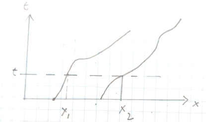
Figure 1: Schematic drawing of two trajectories piercing a time ”plane” which is illustrated as a straight line.

Thus one can define a velocity $\vec{v}_{n}\equiv\frac{d\vec{x}_{n}}{dt}$. The action and Lagrangian for each point particle are as before:

$${\cal A}_{n} = -m_{n}c\int d\tau_{n}-e_{n}\int A^{\alpha}(x^{\nu}_{n})dx_{\alpha n}=\int_{t1}^{t2}L_{n}dt,\qquad L_{n}\equiv L_{0n}+L_{in}$$

$$L_{0n} \equiv -\frac{m_{n}c^{2}}{\gamma_{n}}\simeq\frac{1}{2}m_{n}v_{n}^{2}-m_{n}c^{2},\quad L_{in}\equiv e_{n}\left(\vec{A}(\vec{x}_{n},t)\cdot\vec{v}_{n}-\phi(\vec{x}_{n},t)\right).$$ (13)

The action and Lagrangian of the system of particles is:

$${\cal A}_{s}=\int_{t1}^{t2}L_{s}dt,\qquad L_{s}=\sum_{n=1}^{N}L_{n}.$$ (14)

The variational analysis follows the same lines as for a single particle and we obtain a set of equations of the four dimensional form:

$$m_{n}\frac{du_{n}^{\alpha}}{d\tau_{n}}=-\frac{e_{n}}{c}u_{n}^{\beta}(\partial_{\beta}A_{n}^{\alpha}-\partial^{\alpha}A_{\beta n}),\qquad n\in[1-N].$$ (15)

Or the three dimensional form:

$$\frac{d}{dt}(\gamma_{n}\vec{v}_{n})=\frac{e_{n}}{m_{n}}\left[\vec{v}_{n}\times\vec{B}(\vec{x}_{n},t)+\vec{E}(\vec{x}_{n},t)\right],\qquad n\in[1-N].$$ (16)

in which we do not sum over repeated Latin indices

3 A Relativistic Charged Fluid - the Lagrangian Approach

3.1 The Action and Lagrangian

The dynamics of the fluid is determined by its composition and the forces acting on it. The fluid is made of ”fluid elements” [27, 28], practically a ”fluid element” is a point particle which has an infinitesimal mass $dM_{\vec{\alpha}}$, infinitesimal charge $dQ_{\vec{\alpha}}$, position four vector $x_{\vec{\alpha}\nu}(\tau_{\vec{\alpha}})$ and $u_{\vec{\alpha}\nu}(\tau_{\vec{\alpha}})\equiv\frac{dx_{\vec{\alpha}\nu}(\tau_{\vec{\alpha}})}{d\tau_{\vec{\alpha}}}$. Here the continuous vector label ${\vec{\alpha}}$ replaces the discrete index $n$ of the previous section. As the ”fluid element” is not truly a point particle it has also an infinitesimal volume $dV_{\vec{\alpha}}$, infinitesimal entropy $dS_{\vec{\alpha}}$, and an infinitesimal internal energy $dE_{in~{}\vec{\alpha}}$. The action for each ”fluid element” are according to equation (11) as follows:

$$d{\cal A}_{{\vec{\alpha}}}=-dM_{{\vec{\alpha}}}c\int d\tau_{{\vec{\alpha}}}-dQ_{{\vec{\alpha}}}\int A^{\mu}(x^{\nu}_{{\vec{\alpha}}})dx_{\mu{\vec{\alpha}}}+d{\cal A}_{in~{}{\vec{\alpha}}},$$

$$d{\cal A}_{in~{}{\vec{\alpha}}}\equiv-\int dE_{in~{}{\vec{\alpha}}}dt.$$ (17)

The Lagrangian for each ”fluid element” can be derived from the above expression as follows:

$$d{\cal A}_{{\vec{\alpha}}} = \int_{t1}^{t2}dL_{{\vec{\alpha}}}dt,\qquad dL_{{\vec{\alpha}}}\equiv dL_{k{\vec{\alpha}}}+dL_{i{\vec{\alpha}}}-dE_{in~{}{\vec{\alpha}}}$$

$$dL_{k{\vec{\alpha}}} \equiv -\frac{dM_{{\vec{\alpha}}}c^{2}}{\gamma_{\vec{\alpha}}}\simeq\frac{1}{2}dM_{{\vec{\alpha}}}~{}v_{\vec{\alpha}}(t)^{2}-dM_{{\vec{\alpha}}}c^{2}$$

$$dL_{i{\vec{\alpha}}} \equiv dQ_{{\vec{\alpha}}}\left(\vec{A}(\vec{x}_{\vec{\alpha}}(t),t)\cdot\vec{v}_{\vec{\alpha}}(t)-\phi(\vec{x}_{\vec{\alpha}}(t),t)\right).$$ (18)

all the above quantities are calculated for a specific value of the label ${\vec{\alpha}}$, while the action and Lagrangian of the entire fluid, should be summed (or integrated) over all possible $\vec{\alpha}$’s. That is:

$$L = \int_{{\vec{\alpha}}}dL_{\vec{\alpha}}$$

$${\cal A} = \int_{{\vec{\alpha}}}d{\cal A}_{\vec{\alpha}}=\int_{{\vec{\alpha}}}\int_{t1}^{t2}dL_{\vec{\alpha}}dt=\int_{t1}^{t2}\int_{{\vec{\alpha}}}dL_{\vec{\alpha}}dt=\int_{t1}^{t2}Ldt.$$ (19)

It is customary to define densities for the Lagrangian, mass and charge of every fluid element as follows:

$${\cal L}_{{\vec{\alpha}}}\equiv\frac{dL_{{\vec{\alpha}}}}{dV_{{\vec{\alpha}}}},\quad\rho_{{\vec{\alpha}}}\equiv\frac{dM_{{\vec{\alpha}}}}{dV_{{\vec{\alpha}}}},\quad\rho_{c{\vec{\alpha}}}\equiv\frac{dQ_{{\vec{\alpha}}}}{dV_{{\vec{\alpha}}}},\quad e_{in~{}{\vec{\alpha}}}\equiv\frac{dE_{in~{}{\vec{\alpha}}}}{dV_{{\vec{\alpha}}}}$$ (20)

Each of the above quantities may be thought of as a function of the location $\vec{x}$, where the ”fluid element” labelled ${\vec{\alpha}}$ happens to be in time $t$, for example:

$$\rho(\vec{x},t)\equiv\rho(\vec{x}_{\vec{\alpha}}(t),t)\equiv\rho_{{\vec{\alpha}}}(t)$$ (21)

It is also customary to define the specific internal energy $\varepsilon_{{\vec{\alpha}}}$ as follows:

$$\varepsilon_{{\vec{\alpha}}}\equiv\frac{dE_{in~{}{\vec{\alpha}}}}{dM_{{\vec{\alpha}}}}\quad\Rightarrow\quad\rho_{{\vec{\alpha}}}\varepsilon_{{\vec{\alpha}}}=\frac{dM_{{\vec{\alpha}}}}{dV_{{\vec{\alpha}}}}\frac{dE_{in~{}{\vec{\alpha}}}}{dM_{{\vec{\alpha}}}}=\frac{dE_{in~{}{\vec{\alpha}}}}{dV_{{\vec{\alpha}}}}=e_{in~{}{\vec{\alpha}}}$$ (22)

Thus we can write the following equations for the Lagrangian density:

$${\cal L}_{{\vec{\alpha}}} = \frac{dL_{{\vec{\alpha}}}}{dV_{{\vec{\alpha}}}}=\frac{{dL}_{k{\vec{\alpha}}}}{dV_{{\vec{\alpha}}}}+\frac{{dL}_{i{\vec{\alpha}}}}{dV_{{\vec{\alpha}}}}-\frac{dE_{in~{}{\vec{\alpha}}}}{dV_{{\vec{\alpha}}}}={\cal L}_{k{\vec{\alpha}}}+{\cal L}_{i{\vec{\alpha}}}-e_{in~{}{\vec{\alpha}}}$$

$${\cal L}_{k{\vec{\alpha}}} \equiv -\frac{\rho_{{\vec{\alpha}}}c^{2}}{\gamma_{\vec{\alpha}}}\simeq\frac{1}{2}\rho_{{\vec{\alpha}}}v_{\vec{\alpha}}(t)^{2}-\rho_{{\vec{\alpha}}}c^{2},$$

$${\cal L}_{i{\vec{\alpha}}} \equiv \rho_{c{\vec{\alpha}}}\left(\vec{A}(\vec{x}_{\vec{\alpha}}(t),t)\cdot\vec{v}_{\vec{\alpha}}(t)-\varphi(\vec{x}_{\vec{\alpha}}(t),t)\right).$$ (23)

The above expression allows us to write the Lagrangian as a spatial integral:

$$L=\int_{{\vec{\alpha}}}dL_{\vec{\alpha}}=\int_{{\vec{\alpha}}}{\cal L}_{{\vec{\alpha}}}dV_{{\vec{\alpha}}}=\int{\cal L}(\vec{x},t)d^{3}x$$ (24)

which will be important for later sections of the current paper.

3.2 Variational Analysis

Returning now to the variational analysis we introduce the symbols $\Delta\vec{x}_{{\vec{\alpha}}}\equiv\vec{\xi}_{{\vec{\alpha}}}$ to indicate a variation of the trajectory $\vec{x}_{{\vec{\alpha}}}(t)$ (we reserve the symbol $\delta$ in the fluid context, to a different kind of variation, the Eulerian variation to be described in the next section). Notice that:

$$\Delta\vec{v}_{\vec{\alpha}}(t)=\Delta\frac{d\vec{x}_{\vec{\alpha}}(t)}{dt}=\frac{d\Delta\vec{x}_{\vec{\alpha}}(t)}{dt}=\frac{d\vec{\xi}_{\vec{\alpha}}(t)}{dt}.$$ (25)

And thus according to equation (9):

$$\Delta\left(\frac{1}{\gamma_{\vec{\alpha}}}\right)=-\frac{\gamma_{\vec{\alpha}}\vec{v}_{\vec{\alpha}}(t)}{c^{2}}\frac{d\vec{\xi}_{\vec{\alpha}}(t)}{dt},\qquad\Delta\gamma_{\vec{\alpha}}=\frac{\gamma_{\vec{\alpha}}^{3}\vec{v}_{\vec{\alpha}}(t)}{c^{2}}\frac{d\vec{\xi}_{\vec{\alpha}}(t)}{dt}.$$ (26)

In an ideal fluid the ”fluid element” does exchange mass, nor electric charge, nor heat with other fluid elements, so it follows that:

$$\Delta dM_{\vec{\alpha}}=\Delta dQ_{\vec{\alpha}}=\Delta dS_{\vec{\alpha}}=0.$$ (27)

Moreover, according to thermodynamics a change in the internal energy of a ”fluid element” satisfies the equation in the particle’s rest frame:

$$\Delta dE_{in~{}\vec{\alpha}0}=T_{{\vec{\alpha}}0}\Delta dS_{\vec{\alpha}0}-P_{{\vec{\alpha}}0}\Delta dV_{\vec{\alpha}0},$$ (28)

the first term describes the heating energy gained by the ”fluid element” while the second terms describes the work done by the ”fluid element” on neighbouring elements. $T_{{\vec{\alpha}}0}$ is the temperature of the ”fluid element” and $P_{{\vec{\alpha}}0}$ is the pressure of the same. As the rest mass of the fluid element does not change and does not depend on any specific frame we may divide the above expression by $dM_{\vec{\alpha}}$ to obtain the variation of the specific energy as follows:

$$\Delta\varepsilon_{{\vec{\alpha}}0} = \Delta\frac{dE_{in~{}\vec{\alpha}0}}{dM_{{\vec{\alpha}}}}=T_{{\vec{\alpha}}0}\Delta\frac{dS_{\vec{\alpha}0}}{dM_{{\vec{\alpha}}}}-P_{{\vec{\alpha}}0}\Delta\frac{dV_{\vec{\alpha}0}}{dM_{{\vec{\alpha}}}}$$ (29)

$$= T_{{\vec{\alpha}}0}\Delta s_{{\vec{\alpha}}0}-P_{{\vec{\alpha}}0}\Delta\frac{1}{\rho_{{\vec{\alpha}}0}}=T_{{\vec{\alpha}}0}\Delta s_{{\vec{\alpha}}0}+\frac{P_{{\vec{\alpha}}0}}{\rho_{{\vec{\alpha}}0}^{2}}\Delta\rho_{{\vec{\alpha}}0}.\quad s_{{\vec{\alpha}}0}\equiv\frac{dS_{\vec{\alpha}0}}{dM_{{\vec{\alpha}}}}$$

in which $s_{{\vec{\alpha}}0}$ is the specific entropy of the fluid element in its rest frame. It follows that:

$$\frac{\partial\varepsilon_{0}}{\partial s_{0}}=T_{0},\qquad\frac{\partial\varepsilon_{0}}{\partial\rho_{0}}=\frac{P_{0}}{\rho_{0}^{2}}.$$ (30)

Another important thermodynamic quantity that we will use later is the Enthalpy defined for a fluid element in its rest frame as:

$$dW_{{\vec{\alpha}}0}=dE_{in~{}\vec{\alpha}0}+P_{{\vec{\alpha}}0}dV_{{\vec{\alpha}}0}.$$ (31)

and the specific enthalpy:

$$w_{{\vec{\alpha}}0}=\frac{dW_{{\vec{\alpha}}0}}{dM_{{\vec{\alpha}}}}=\frac{dE_{in~{}\vec{\alpha}0}}{dM_{{\vec{\alpha}}}}+P_{{\vec{\alpha}}0}\frac{dV_{{\vec{\alpha}}0}}{dM_{{\vec{\alpha}}}}=\varepsilon_{{\vec{\alpha}}0}+\frac{P_{{\vec{\alpha}}0}}{\rho_{{\vec{\alpha}}0}}.$$ (32)

Combining the above result with equation (30) it follows that:

$$w_{0}=\varepsilon_{0}+\frac{P_{0}}{\rho_{0}}=\varepsilon_{0}+\rho_{0}\frac{\partial\varepsilon_{0}}{\partial\rho_{0}}=\frac{\partial(\rho_{0}\varepsilon_{0})}{\partial\rho_{0}}.$$ (33)

Moreover:

$$\frac{\partial w_{0}}{\partial\rho_{0}}=\frac{\partial(\varepsilon_{0}+\frac{P_{0}}{\rho_{0}})}{\partial\rho_{0}}=-\frac{P_{0}}{\rho_{0}^{2}}+\frac{1}{\rho_{0}}\frac{\partial P_{0}}{\partial\rho_{0}}+\frac{\partial\varepsilon_{0}}{\partial\rho_{0}}=-\frac{P_{0}}{\rho_{0}^{2}}+\frac{1}{\rho_{0}}\frac{\partial P_{0}}{\partial\rho_{0}}+\frac{P_{0}}{\rho_{0}^{2}}=\frac{1}{\rho_{0}}\frac{\partial P_{0}}{\partial\rho_{0}}.$$ (34)

As we assume an ideal fluid, there is no heat conduction or heat radiation, and thus heat can only be moved around along the trajectory of the ”fluid elements”, that is only convection is taken into account. Thus $\Delta dS_{\vec{\alpha}0}=0$ and we have:

$$\Delta dE_{in~{}\vec{\alpha}0}=-P_{0}\Delta dV_{\vec{\alpha}0}.$$ (35)

Our next step would to be to evaluate the variation of the volume element. However, before we do this we establish some relations between the rest frame and any other frame in which the fluid element is in motion (this frame is sometimes denoted the ”laboratory” frame). First we notice that at the rest frame there is no velocity (by definition), hence according to equation (9):

$$d\tau=cdt_{0}=cdt\sqrt{1-\frac{v^{2}}{c^{2}}}=\frac{cdt}{\gamma}\quad\Rightarrow\quad dt_{0}=\frac{dt}{\gamma}.$$ (36)

It is well known that the four volume is Lorentz invariant, hence:

$$dV_{0}dt_{0}=dVdt=dVdt_{0}\gamma,\qquad\Rightarrow dV_{0}=\gamma dV.$$ (37)

Thus:

$$\rho_{0}=\frac{dM}{dV_{0}}=\frac{1}{\gamma}\frac{dM}{dV}=\frac{\rho}{\gamma},\qquad\Rightarrow\quad\rho=\gamma\rho_{0}.$$ (38)

Moreover, the action given in equation (17) is Lorentz invariant, thus:

$$dE_{in~{}{\vec{\alpha}}0}dt_{0}=dE_{in~{}{\vec{\alpha}}}dt=dE_{in~{}{\vec{\alpha}}}dt_{0}\gamma\Rightarrow dE_{in~{}{\vec{\alpha}}0}=\gamma dE_{in~{}{\vec{\alpha}}},dE_{in~{}{\vec{\alpha}}}=\frac{dE_{in~{}{\vec{\alpha}}0}}{\gamma}$$ (39)

We are now at a position to calculate the variation of the internal energy of a fluid element:

$$\Delta dE_{in~{}{\vec{\alpha}}}=\Delta\left(\frac{1}{\gamma}\right)dE_{in~{}{\vec{\alpha}}0}+\frac{1}{\gamma}\Delta dE_{in~{}{\vec{\alpha}}0}.$$ (40)

Taking into account equation (35) and equation (37) we obtain:

$$\Delta dE_{in~{}{\vec{\alpha}}}=\Delta\left(\frac{1}{\gamma}\right)dE_{in~{}{\vec{\alpha}}0}-\frac{1}{\gamma}P_{0}\Delta dV_{\vec{\alpha}0}=\Delta\left(\frac{1}{\gamma}\right)dE_{in~{}{\vec{\alpha}}0}-\frac{1}{\gamma}P_{0}\Delta(\gamma dV_{\vec{\alpha}}).$$ (41)

Thus using the definition of enthalpy given in equation (31) we may write:

$$\Delta dE_{in~{}{\vec{\alpha}}}=\Delta\left(\frac{1}{\gamma}\right)(dE_{in~{}{\vec{\alpha}}0}+P_{0}dV_{\vec{\alpha}0})-\ P_{0}\Delta dV_{\vec{\alpha}}=\Delta\left(\frac{1}{\gamma}\right)dW_{{\vec{\alpha}}0}-\ P_{0}\Delta dV_{\vec{\alpha}}.$$ (42)

We shall now calculate the variation of the volume element. Suppose at a time $t$ the volume of the fluid element labelled by ${\vec{\alpha}}$ is described as:

$$dV_{{\vec{\alpha}},t}=d^{3}x({\vec{\alpha}},t)$$ (43)

Using the Jacobian determinant we may relate this to the same element at $t=0$:

$$d^{3}x({\vec{\alpha}},t)=Jd^{3}x({\vec{\alpha}},0),\qquad J\equiv\vec{\nabla}_{0}x_{1}\cdot(\vec{\nabla}_{0}x_{2}\times\vec{\nabla}_{0}x_{3})$$ (44)

In which $\vec{\nabla}_{0}$ is taken with respect to the coordinates of the fluid elements at $t=0$: $\vec{\nabla}_{0}\equiv(\frac{\partial}{\partial x({\vec{\alpha}},0)_{1}},\frac{\partial}{\partial x({\vec{\alpha}},0)_{2}},\frac{\partial}{\partial x({\vec{\alpha}},0)_{3}})$. As both the actual and varied ”fluid element” trajectories start at the same point it follows that:

$$\Delta dV_{{\vec{\alpha}},t} = \Delta d^{3}x({\vec{\alpha}},t)=\Delta J~{}d^{3}x({\vec{\alpha}},0)=\frac{\Delta J}{J}d^{3}x({\vec{\alpha}},t)=\frac{\Delta J}{J}dV_{{\vec{\alpha}},t},$$

$$(\Delta d^{3}x({\vec{\alpha}},0) = 0).$$ (45)

The variation of $J$ can be easily calculated as:

$$\Delta J=\vec{\nabla}_{0}\Delta x_{1}\cdot(\vec{\nabla}_{0}x_{2}\times\vec{\nabla}_{0}x_{3})+\vec{\nabla}_{0}x_{1}\cdot(\vec{\nabla}_{0}\Delta x_{2}\times\vec{\nabla}_{0}x_{3})+\vec{\nabla}_{0}x_{1}\cdot(\vec{\nabla}_{0}x_{2}\times\vec{\nabla}_{0}\Delta x_{3}),$$ (46)

Now:

$$\vec{\nabla}_{0}\Delta x_{1}\cdot(\vec{\nabla}_{0}x_{2}\times\vec{\nabla}_{0}x_{3})=\vec{\nabla}_{0}\xi_{1}\cdot(\vec{\nabla}_{0}x_{2}\times\vec{\nabla}_{0}x_{3})$$ (47)

$$= \partial_{k}\xi_{1}\vec{\nabla}_{0}x_{k}\cdot(\vec{\nabla}_{0}x_{2}\times\vec{\nabla}_{0}x_{3})=\partial_{1}\xi_{1}\vec{\nabla}_{0}x_{1}\cdot(\vec{\nabla}_{0}x_{2}\times\vec{\nabla}_{0}x_{3})=\partial_{1}\xi_{1}J.$$

$$\vec{\nabla}_{0}x_{1}\cdot(\vec{\nabla}_{0}\Delta x_{2}\times\vec{\nabla}_{0}x_{3})=\vec{\nabla}_{0}x_{1}\cdot(\vec{\nabla}_{0}\xi_{2}\times\vec{\nabla}_{0}x_{3})$$

$$= \partial_{k}\xi_{2}\vec{\nabla}_{0}x_{1}\cdot(\vec{\nabla}_{0}x_{k}\times\vec{\nabla}_{0}x_{3})=\partial_{2}\xi_{2}\vec{\nabla}_{0}x_{1}\cdot(\vec{\nabla}_{0}x_{2}\times\vec{\nabla}_{0}x_{3})=\partial_{2}\xi_{2}J.$$

$$\vec{\nabla}_{0}x_{1}\cdot(\vec{\nabla}_{0}x_{2}\times\vec{\nabla}_{0}\Delta x_{3})=\vec{\nabla}_{0}x_{1}\cdot(\vec{\nabla}_{0}x_{2}\times\vec{\nabla}_{0}\xi_{3})$$

$$= \partial_{k}\xi_{3}\vec{\nabla}_{0}x_{1}\cdot(\vec{\nabla}_{0}x_{2}\times\vec{\nabla}_{0}x_{k})=\partial_{3}\xi_{3}\vec{\nabla}_{0}x_{1}\cdot(\vec{\nabla}_{0}x_{2}\times\vec{\nabla}_{0}x_{3})=\partial_{3}\xi_{3}J.$$

Combining the above results, it follows that:

$$\Delta J=\partial_{1}\xi_{1}J+\partial_{2}\xi_{2}J+\partial_{3}\xi_{3}J=\vec{\nabla}\cdot\vec{\xi}~{}J.$$ (48)

Which allows us to calculate the variation of the volume of the ”fluid element”:

$$\Delta dV_{{\vec{\alpha}},t}=\vec{\nabla}\cdot\vec{\xi}~{}dV_{{\vec{\alpha}},t}.$$ (49)

And thus the variation of the internal energy given in equation (42) is:

$$\Delta dE_{in~{}\vec{\alpha}}=\Delta\left(\frac{1}{\gamma}\right)dW_{{\vec{\alpha}}0}-P_{0}\vec{\nabla}\cdot\vec{\xi}~{}dV_{{\vec{\alpha}},t}.$$ (50)

Taking into account equation (26) this takes the form:

$$\Delta dE_{in~{}\vec{\alpha}}=-P_{{\vec{\alpha}}0}\vec{\nabla}\cdot\vec{\xi}_{\vec{\alpha}}~{}dV_{{\vec{\alpha}},t}-\frac{\gamma_{\vec{\alpha}}\vec{v}_{\vec{\alpha}}(t)}{c^{2}}dW_{{\vec{\alpha}}0}\cdot\frac{d\vec{\xi}_{\vec{\alpha}}(t)}{dt}.$$ (51)

The variation of internal energy is the only novel element with respect to the system of particles scenario described in the previous section, thus the rest of the variation analysis is straight forward. Varying equation (17) we obtain:

$$\Delta d{\cal A}_{{\vec{\alpha}}} = \int_{t1}^{t2}\Delta dL_{{\vec{\alpha}}}dt,\qquad\Delta dL_{{\vec{\alpha}}}=\Delta dL_{k{\vec{\alpha}}}+\Delta dL_{i{\vec{\alpha}}}-\Delta dE_{in~{}{\vec{\alpha}}}$$

$$\Delta dL_{k{\vec{\alpha}}} = -dM_{{\vec{\alpha}}}c^{2}\Delta\left(\frac{1}{\gamma_{\vec{\alpha}}}\right)=dM_{{\vec{\alpha}}}\gamma_{\vec{\alpha}}\vec{v}_{\vec{\alpha}}(t)\cdot\frac{d\vec{\xi}_{\vec{\alpha}}(t)}{dt},$$

$$\Delta dL_{i{\vec{\alpha}}} = dQ_{{\vec{\alpha}}}\left(\Delta\vec{A}(\vec{x}_{\vec{\alpha}}(t),t)\cdot\vec{v}_{\vec{\alpha}}(t)+\vec{A}(\vec{x}_{\vec{\alpha}}(t),t)\cdot\Delta\vec{v}_{\vec{\alpha}}(t)\right.$$ (52)

$$- \left.\Delta\phi(\vec{x}_{\vec{\alpha}}(t),t)\right).$$

We can now combine the internal and kinetic parts of the varied Lagrangian taking into account the specific enthalpy definition given in equation (32):

$$\Delta dL_{k{\vec{\alpha}}}-\Delta dE_{in~{}{\vec{\alpha}}}=dM_{{\vec{\alpha}}}\gamma_{\vec{\alpha}}(\left(1+\frac{w_{0}}{c^{2}}\right)\vec{v}_{\vec{\alpha}}(t)\cdot\frac{d\vec{\xi}_{\vec{\alpha}}(t)}{dt}+P_{{\vec{\alpha}}0}\vec{\nabla}\cdot\vec{\xi}_{{\vec{\alpha}}}~{}dV_{{\vec{\alpha}},t}.$$ (53)

The electromagnetic interaction variation terms are not different than in the low speed (non-relativistic) case, see for example equations A47 and A48 of [50], and their derivation will not be repeated here:

$$d\vec{F}_{L{\vec{\alpha}}}\equiv dQ_{{\vec{\alpha}}}\left[\vec{v}_{{\vec{\alpha}}}\times\vec{B}(\vec{x}_{\vec{\alpha}}(t),t)+\vec{E}(\vec{x}_{\vec{\alpha}}(t),t)\right]$$ (54)

and:

$$\Delta dL_{i{\vec{\alpha}}}=\frac{d(dQ_{{\vec{\alpha}}}\vec{A}(\vec{x}_{\vec{\alpha}}(t),t)\cdot\vec{\xi}_{{\vec{\alpha}}})}{dt}+d\vec{F}_{L{\vec{\alpha}}}\cdot\vec{\xi}_{{\vec{\alpha}}}.$$ (55)

Introducing the shorthand notation:

$$\bar{\lambda}\equiv 1+\frac{w_{0}}{c^{2}},\qquad\lambda\equiv\gamma\bar{\lambda}=\gamma\left(1+\frac{w_{0}}{c^{2}}\right).$$ (56)

The variation of the action of a relativistic single fluid element is thus:

$$\Delta d{\cal A}_{{\vec{\alpha}}} = \int_{t1}^{t2}\Delta dL_{{\vec{\alpha}}}dt=\left.(dM_{{\vec{\alpha}}}\lambda_{\vec{\alpha}}\vec{v}_{\vec{\alpha}}(t)+dQ_{{\vec{\alpha}}}\vec{A}(\vec{x}_{\vec{\alpha}}(t),t))\cdot\vec{\xi}_{{\vec{\alpha}}}\right|_{t1}^{t2}$$ (57)

$$- \int_{t1}^{t2}(dM_{{\vec{\alpha}}}\frac{d(\lambda_{\vec{\alpha}}\vec{v}_{\vec{\alpha}}(t))}{dt}\cdot\vec{\xi}_{{\vec{\alpha}}}-d\vec{F}_{L{\vec{\alpha}}}\cdot\vec{\xi}_{{\vec{\alpha}}}-P_{{\vec{\alpha}}0}\vec{\nabla}\cdot\vec{\xi}_{{\vec{\alpha}}}~{}dV_{{\vec{\alpha}},t})dt.$$

The variation of the total action of the fluid is thus:

$$\Delta{\cal A} = \int_{{\vec{\alpha}}}d{\cal A}_{\vec{\alpha}}=\left.\int_{{\vec{\alpha}}}(dM_{{\vec{\alpha}}}\lambda_{\vec{\alpha}}\vec{v}_{\vec{\alpha}}(t)+dQ_{{\vec{\alpha}}}\vec{A}(\vec{x}({\vec{\alpha}},t),t))\cdot\vec{\xi}_{{\vec{\alpha}}}\right|_{t1}^{t2}$$ (58)

$$- \int_{t1}^{t2}\int_{{\vec{\alpha}}}(dM_{{\vec{\alpha}}}\frac{d(\lambda_{\vec{\alpha}}\vec{v}_{\vec{\alpha}}(t))}{dt}\cdot\vec{\xi}_{{\vec{\alpha}}}-d\vec{F}_{L{\vec{\alpha}}}\cdot\vec{\xi}_{{\vec{\alpha}}}-P_{{\vec{\alpha}}0}\vec{\nabla}\cdot\vec{\xi}_{{\vec{\alpha}}}~{}dV_{{\vec{\alpha}}})dt.$$

Now according to equation (20) we may write:

$$dM_{{\vec{\alpha}}}=\rho_{{\vec{\alpha}}}~{}dV_{{\vec{\alpha}}},\qquad dQ_{{\vec{\alpha}}}=\rho_{c{\vec{\alpha}}}~{}dV_{{\vec{\alpha}}}$$ (59)

using the above relations we may turn the ${\vec{\alpha}}$ integral into a volume integral and thus write the variation of the fluid action in which we suppress the ${\vec{\alpha}}$ labels:

$$\Delta{\cal A}=\left.\int(\rho\lambda\vec{v}+\rho_{c}\vec{A})\cdot\vec{\xi}dV\right|_{t1}^{t2}-\int_{t1}^{t2}\int(\rho\frac{d(\lambda\vec{v})}{dt}\cdot\vec{\xi}-\vec{f}_{L}\cdot\vec{\xi}-P_{0}\vec{\nabla}\cdot\vec{\xi})dVdt.$$ (60)

in the above we introduced the Lorentz force density:

$$\vec{f}_{L{\vec{\alpha}}}\equiv\frac{d\vec{F}_{L{\vec{\alpha}}}}{dV_{{\vec{\alpha}}}}=\rho_{c{\vec{\alpha}}}\left[\vec{v}_{{\vec{\alpha}}}\times\vec{B}(\vec{x}_{\vec{\alpha}}(t),t)+\vec{E}(\vec{x}_{\vec{\alpha}}(t),t)\right].$$ (61)

Now, since:

$$P_{0}\vec{\nabla}\cdot\vec{\xi}=\vec{\nabla}\cdot(P_{0}\vec{\xi})-\vec{\xi}\cdot\vec{\nabla}P_{0},$$ (62)

and using Gauss theorem the variation of the action can be written as:

$$\Delta{\cal A} = \left.\int(\rho\lambda\vec{v}+\rho_{c}\vec{A})\cdot\vec{\xi}dV\right|_{t1}^{t2}$$ (63)

$$- \int_{t1}^{t2}\left[\int(\rho\frac{d(\lambda\vec{v})}{dt}-\vec{f}_{L}+\vec{\nabla}P_{0})\cdot\vec{\xi}dV-\oint P_{0}\vec{\xi}\cdot d\vec{\Sigma}\right]dt.$$

It follows that the variation of the action will vanish for a $\vec{\xi}$ such that $\vec{\xi}(t1)=\vec{\xi}(t2)=0$ and vanishing on a surface encapsulating the fluid, but other than that arbitrary only if the Euler equation for a relativistic charged fluid is satisfied, that is:

$$\frac{d(\lambda\vec{v})}{dt}=-\frac{\vec{\nabla}P_{0}}{\rho}+\frac{\vec{f}_{L}}{\rho}$$ (64)

for the particular case that the fluid element is made of identical microscopic particles each with a mass $m$ and a charge $e$, it follows that the mass and charge densities are proportional to the number density $n$:

$$\rho=m~{}n,\quad\rho_{c}=e~{}n\Rightarrow\frac{\vec{f}_{L}}{\rho}=k\left[\vec{v}\times\vec{B}+\vec{E}\right],k\equiv\frac{e}{m}$$ (65)

thus except from the terms related to the internal energy the equation is similar to that of a point particle. For a neutral fluid one obtains the form:

$$\frac{d(\lambda\vec{v})}{dt}=-\frac{\vec{\nabla}P_{0}}{\rho}.$$ (66)

Some authors prefer to write the above equation in terms of the energy per element of the fluid per unit volume in the rest frame which is the sum of the internal energy contribution and the rest mass contribution:

$$e_{0}\equiv\rho_{0}c^{2}+\rho_{0}\varepsilon_{0}.$$ (67)

It is easy to show that:

$$\bar{\lambda}=1+\frac{w_{0}}{c^{2}}=\frac{e_{0}+P_{0}}{\rho_{0}c^{2}}.$$ (68)

And using the above equality and some manipulations we may write equation (66) in a form which is preferable by some authors:

$$(e_{0}+P_{0})\frac{\gamma}{c^{2}}\frac{d(\gamma\vec{v})}{dt}=-\vec{\nabla}P_{0}-\frac{\gamma^{2}}{c^{2}}\frac{dP_{0}}{dt}\vec{v}.$$ (69)

In experimental fluid dynamics it is more convenient to describe a fluid in terms of quantities at a specific location, rather than quantities associated with unseen infinitesimal ”fluid elements”. This road leads to the Eulerian description of fluid dynamics and thinking in terms of flow fields rather than in terms of a velocity of ”fluid elements” as will be discussed in the next section.

4 An Eulerian Charged Fluid - the Clebsch Approach

In this section we follows closely the analysis of [23, 50, 51] with the modification of taking into account the relativistic corrections, this implies taking into account an action which is invariant under Lorentz transformations. Let us consider the action:

$${\cal A} \equiv \int{\cal L}d^{3}xdt,\qquad{\cal L}\equiv{\cal L}_{0}+{\cal L}_{2}+{\cal L}_{i}$$

$${\cal L}_{0} \equiv -\rho(\frac{c^{2}}{\gamma}+\varepsilon)=-\rho_{0}(c^{2}+\varepsilon_{0})=-e_{0},\qquad{\cal L}_{2}\equiv\nu\partial^{\nu}(\rho_{0}u_{\nu})-\rho_{0}\alpha u_{\nu}\partial^{\nu}\beta,$$

$${\cal L}_{i} \equiv -\rho_{c}A^{\nu}v_{\nu},\qquad v_{\nu}\equiv\frac{dx_{\nu}}{dt}.$$ (70)

In the non relativistic limit we may write:

$${\cal L}_{0}\simeq\rho(\frac{1}{2}v^{2}-\varepsilon-c^{2})$$ (71)

Taking into account that:

$$u_{\mu}=\gamma(c,\vec{v})$$ (72)

and also that $\rho=\gamma\rho_{0}$ according to equation (38), it is easy to write the above Lagrangian densities in a space-time formalism:

$${\cal L}_{2}=\nu[\frac{\partial{\rho}}{\partial t}+\vec{\nabla}\cdot(\rho\vec{v})]-\rho\alpha\frac{d\beta}{dt}\qquad{\cal L}_{i}=\rho_{c}\left(\vec{A}\cdot\vec{v}-\phi\right)$$ (73)

In the Eulerian approach we consider the variational variables to be fields, that functions of space and time. We have two such variational variables the vector velocity field $\vec{v}(\vec{x},t)$ and density scalar field $\rho(\vec{x},t)$. The conservation of quantities such as the label of the fluid element, mass, charge and entropy are dealt by introducing Lagrange multipliers $\nu,\alpha$ in such a way that the variational principle will yield the following equations:

$$\frac{\partial{\rho}}{\partial t}+\vec{\nabla}\cdot(\rho\vec{v})=0$$

$$\frac{d\beta}{dt}=0$$ (74)

Provided $\rho$ is not null those are just the continuity equation which ensures mass conservation and the conditions that $\beta$ is comoving and is thus a label. Let us now calculate the variation with respect to $\beta$, this will lead us to the following results:

$$\delta_{\beta}A = \int d^{3}xdt\delta\beta[\frac{\partial{(\rho\alpha)}}{\partial t}+\vec{\nabla}\cdot(\rho\alpha\vec{v})]$$ (75)

$$- \oint d\vec{S}\cdot\vec{v}\rho\alpha\delta\beta-\int d\vec{\Sigma}\cdot\vec{v}\rho\alpha[\delta\beta]-\int d^{3}x\rho\alpha\delta\beta|^{t_{1}}_{t_{0}}$$

Hence choosing $\delta\beta$ in such a way that the temporal and spatial boundary terms vanish (this includes choosing $\delta\beta$ to be continuous on the cut if one needs to introduce such a cut) in the above integral will lead to the equation:

$$\frac{\partial{(\rho\alpha)}}{\partial t}+\vec{\nabla}\cdot(\rho\alpha\vec{v})=0$$ (76)

Using the continuity equation (74) this will lead to the equation:

$$\frac{d\alpha}{dt}=0$$ (77)

Hence for $\rho\neq 0$ both $\alpha$ and $\beta$ are comoving coordinates. This is why in the Eulerian approach we are obliged to add the Lagrangian density ${\cal L}_{2}$. The specific internal energy $\varepsilon_{0}$ defined in equation (22) is dependent on the thermodynamic properties of the specific fluid. That is it generally depends through a given ”equation of state” on the density and specific entropy. In our case we shall assume a barotropic fluid, that is a fluid in which $\varepsilon_{0}(\rho_{0})$ is a function of the density $\rho_{0}$ only. Other functions connected to the electromagnetic interaction such as the potentials $\vec{A},\phi$ are assumed given function of coordinates and are not varied. Another simplification which we introduce is the assumption the fluid element is made of microscopic particles having a given mass $m$ and a charge $e$, in this case it follows from equation (65) that:

$$\rho_{c}=k\rho.$$ (78)

Let us now take the variational derivative with respect to the density $\rho$, we obtain:

$$\delta_{\rho}A = \int d^{3}xdt\delta\rho[-\frac{c^{2}}{\gamma}-w_{0}\frac{\delta\rho_{0}}{\delta\rho}-\frac{\partial{\nu}}{\partial t}-\vec{v}\cdot\vec{\nabla}\nu+k(\vec{A}\cdot\vec{v}-\phi)]$$ (79)

$$+ \oint d\vec{S}\cdot\vec{v}\delta\rho\nu+\int d\vec{\Sigma}\cdot\vec{v}\delta\rho[\nu]+\int d^{3}x\nu\delta\rho|^{t_{1}}_{t_{0}}$$

Or as:

$$\delta_{\rho}A = \int d^{3}xdt\delta\rho[-\frac{c^{2}+w_{0}}{\gamma}-\frac{\partial{\nu}}{\partial t}-\vec{v}\cdot\vec{\nabla}\nu+k(\vec{A}\cdot\vec{v}-\phi)]$$ (80)

$$+ \oint d\vec{S}\cdot\vec{v}\delta\rho\nu+\int d\vec{\Sigma}\cdot\vec{v}\delta\rho[\nu]+\int d^{3}x\nu\delta\rho|^{t_{1}}_{t_{0}}$$

in which $w_{0}=\frac{\partial(\rho_{0}\varepsilon_{0})}{\partial\rho_{0}}$ is the specific enthalpy in the rest frame of the fluid element (see equation (33)). Hence provided that $\delta\rho$ vanishes on the boundary of the domain, on the cut and in initial and final times the following equation must be satisfied:

$$\frac{d\nu}{dt}=\frac{\partial\nu}{\partial t}+\vec{v}\cdot\vec{\nabla}\nu=-\frac{c^{2}+w_{0}}{\gamma}+k(\vec{A}\cdot\vec{v}-\phi)$$ (81)

In the above we notice that taking a time derivative for a fixed label ${\vec{\alpha}}$ (also known as a material derivative) of any quantity $g$ takes the form:

$$\frac{dg({\vec{\alpha}},t)}{dt}=\frac{dg(\vec{x}({\vec{\alpha}},t),t)}{dt}=\frac{\partial g}{\partial t}+\frac{d\vec{x}}{dt}\cdot\vec{\nabla}g=\frac{\partial g}{\partial t}+\vec{v}\cdot\vec{\nabla}g$$ (82)

once $g$ is considered to be a field dependent on $\vec{x},t$.

Finally Let us take an arbitrary variational derivative of the above action with respect to $\vec{v}$, taking into account that:

$$\delta_{\vec{v}}\frac{1}{\gamma}=-\gamma\frac{\vec{v}\cdot\delta\vec{v}}{c^{2}}$$ (83)

This will result in:

$$\delta_{\vec{v}}A = \int d^{3}xdt\rho\delta\vec{v}\cdot[\gamma\vec{v}-\frac{w_{0}}{\rho}\frac{\delta\rho_{0}}{\delta\vec{v}}-\vec{\nabla}\nu-\alpha\vec{\nabla}\beta+k\vec{A}]$$ (84)

$$+ \oint d\vec{S}\cdot\delta\vec{v}\rho\nu+\int d\vec{\Sigma}\cdot\delta\vec{v}\rho[\nu].$$

However:

$$\frac{\delta\rho_{0}}{\delta\vec{v}}=\rho\frac{\delta\frac{1}{\gamma}}{\delta\vec{v}}=-\rho\gamma\frac{\vec{v}}{c^{2}}$$ (85)

Taking in account the definition of $\lambda$ (see equation (56)), we thus have:

$$\delta_{\vec{v}}A = \int d^{3}xdt\rho\delta\vec{v}\cdot[\lambda\vec{v}-\vec{\nabla}\nu-\alpha\vec{\nabla}\beta+k\vec{A}]$$ (86)

$$+ \oint d\vec{S}\cdot\delta\vec{v}\rho\nu+\int d\vec{\Sigma}\cdot\delta\vec{v}\rho[\nu].$$

the above boundary terms contain integration over the external boundary $\oint d\vec{S}$ and an integral over the cut $\int d\vec{\Sigma}$ that must be introduced in case that $\nu$ is not single valued, more on this case in later sections. The external boundary term vanishes; in the case of astrophysical flows for which $\rho=0$ on the free flow boundary, or the case in which the fluid is contained in a vessel which induces a no flux boundary condition $\delta\vec{v}\cdot\hat{n}=0$ ($\hat{n}$ is a unit vector normal to the boundary). The cut ”boundary” term vanish when the velocity field varies only parallel to the cut that is it satisfies a Kutta type condition. If the boundary terms vanish $\vec{v}$ must have the following form:

$$\lambda\vec{v}=\alpha\vec{\nabla}\beta+\vec{\nabla}\nu-k\vec{A}$$ (87)

this is a generalization of Clebsch representation of the flow field (see for example [27], [41, page 248]) for a relativistic charged flow.

4.1 Euler’s equations

We shall now show that a velocity field given by equation (87), such that the functions $\alpha,\beta,\nu$ satisfy the corresponding equations (74,81,77) must satisfy Euler’s equations. Let us calculate the material derivative of $\lambda\vec{v}$:

$$\frac{d(\lambda\vec{v})}{dt}=\frac{d\vec{\nabla}\nu}{dt}+\frac{d\alpha}{dt}\vec{\nabla}\beta+\alpha\frac{d\vec{\nabla}\beta}{dt}-k\frac{d\vec{A}}{dt}$$ (88)

It can be easily shown that:

$$\frac{d\vec{\nabla}\nu}{dt} = \vec{\nabla}\frac{d\nu}{dt}-\vec{\nabla}v_{n}\frac{\partial\nu}{\partial x_{n}}=\vec{\nabla}\left(-\frac{c^{2}+w_{0}}{\gamma}+k\vec{A}\cdot\vec{v}-k\phi\right)-\vec{\nabla}v_{n}\frac{\partial\nu}{\partial x_{n}}$$

$$\frac{d\vec{\nabla}\beta}{dt} = \vec{\nabla}\frac{d\beta}{dt}-\vec{\nabla}v_{n}\frac{\partial\beta}{\partial x_{n}}=-\vec{\nabla}v_{n}\frac{\partial\beta}{\partial x_{n}}$$ (89)

In which $x_{n}$ is a Cartesian coordinate and a summation convention is assumed. Inserting the result from equations (89) into equation (88) yields:

$$\frac{d(\lambda\vec{v})}{dt}=-\vec{\nabla}v_{n}(\frac{\partial\nu}{\partial x_{n}}+\alpha\frac{\partial\beta}{\partial x_{n}})+\vec{\nabla}\left(-\frac{c^{2}+w_{0}}{\gamma}+k\vec{A}\cdot\vec{v}-k\phi\right)-k\frac{d\vec{A}}{dt}$$ (90)

$$= -\vec{\nabla}v_{n}(\lambda v_{n}+kA_{n})+\vec{\nabla}(-\frac{c^{2}+w_{0}}{\gamma}+k\vec{A}\cdot\vec{v}-k\phi)-k\partial_{t}\vec{A}-k(\vec{v}\cdot\vec{\nabla})\vec{A}$$

$$= -\frac{1}{\gamma}\vec{\nabla}w_{0}+k\vec{E}+k(v_{n}\vec{\nabla}A_{n}-v_{n}\partial_{n}\vec{A}),$$

in the above we have used the electric field defined in equation (8). We notice that according to equation (7):

$$(v_{n}\vec{\nabla}A_{n}-v_{n}\partial_{n}\vec{A})_{l}=v_{n}(\partial_{l}A_{n}-\partial_{n}A_{l})=\epsilon_{lnj}v_{n}B_{j}=(\vec{v}\times\vec{B})_{l},$$ (91)

Hence we obtain the Euler equation of a charged relativistic fluid in the form:

$$\frac{d(\lambda\vec{v})}{dt}=-\frac{1}{\gamma}\vec{\nabla}w_{0}+k\left[\vec{v}\times\vec{B}+\vec{E}\right]=-\frac{1}{\rho}\vec{\nabla}P_{0}+k\left[\vec{v}\times\vec{B}+\vec{E}\right],$$ (92)

since (see equation (34)):

$$\vec{\nabla}w_{0}=\frac{\partial w_{0}}{\partial\rho_{0}}\vec{\nabla}\rho_{0}=\frac{1}{\rho_{0}}\frac{\partial P_{0}}{\partial\rho_{0}}\vec{\nabla}\rho_{0}=\frac{1}{\rho_{0}}\vec{\nabla}P_{0}.$$ (93)

The above equation is identical to equation (64) and thus proves that the Euler equations can be derived from the action given in equation (73) and hence all the equations of charged fluid dynamics can be derived from the above action without restricting the variations in any way.

4.2 Simplified action

The reader of this paper might argue that the authors have introduced unnecessary complications to the theory of relativistic fluid dynamics by adding three more functions $\alpha,\beta,\nu$ to the standard set $\vec{v},\rho$. In the following we will show that this is not so and the action given in equation (70) in a form suitable for a pedagogic presentation can indeed be simplified. It is easy to show that defining a four dimensional Clebsch four vector:

$$v_{C}^{\mu}\equiv\alpha\partial^{\mu}\beta+\partial^{\mu}\nu=(\frac{1}{c}(\alpha\partial_{t}\beta+\partial_{t}\nu),\alpha\vec{\nabla}\beta+\vec{\nabla}\nu)=(\frac{1}{c}(\alpha\partial_{t}\beta+\partial_{t}\nu),\vec{v}_{C})$$ (94)

and a four dimensional electromagnetic Clebsch four vector:

$$v_{E}^{\mu}\equiv v_{C}^{\mu}+kA^{\mu}=(\frac{1}{c}(\alpha\partial_{t}\beta+\partial_{t}\nu+k\phi),\vec{v}_{C}-k\vec{A}).$$ (95)

It follows from equation (81) and equation (87) that:

$$v_{\mu}=-\frac{v_{E\mu}}{\lambda}\Rightarrow\vec{v}=\frac{\vec{v}_{E}}{\lambda}.$$ (96)

Eliminating $\vec{v}$ the Lagrangian density appearing in equation (73) can be written (up to surface terms) in the compact form:

$${\cal L}[\rho_{0},\alpha,\beta,\nu]=\rho_{0}\left[c\sqrt{v_{E\mu}v_{E}^{\mu}}-\varepsilon_{0}-c^{2}\right]$$ (97)

This Lagrangian density will yield the four equations (74,77,81), after those equations are solved we can insert the potentials $\alpha,\beta,\nu$ into equation (87) to obtain the physical velocity $\vec{v}$. Hence, the general charged relativistic barotropic fluid dynamics problem is changed such that instead of solving the Euler and continuity equations we need to solve an alternative set which can be derived from the Lagrangian density $\hat{\cal L}$.

5 Conclusion

The current work which is a continuation of previous studies [23, 47, 49] in which we demonstrate how Pauli’s spinor can be interpreted in terms of spin fluid using a generalized Clebsch form which is modified to include the electromagnetic vector potential affecting a charged fluid. The theory is described by an action and a variational principle and the fluid equations are derived as the extrema of the action. The similarities as well as the pronounced differences with barotropic fluid dynamics were discussed.

A fundamental obstacle to the fluid interpretation of quantum mechanics still exist. This is related to the origin of thermodynamic quantities which are part of fluid mechanics in the quantum context. For classical fluid the thermodynamic internal energy implies that a fluid element is not a point particle but has internal structure. In standard thermodynamics notions as specific enthalpy, pressure and temperature are derived from the specific internal energy equation of state. The internal energy is a required component of any Lagrangian density attempting to depict a fluid. The unique form of the internal energy can be derived in principle relying on the basis of the atoms and molecules from which the fluid is composed and their interactions using statistical physics. However, the quantum fluid has no such microscopic structure and yet analysis of both the spin less [6, 7] and spin [23] quantum fluid shows that terms analogue to internal energies appear. Thus one is forced to ask where do those internal energies originate, surely the quantum fluid is devoid of a microscopic sub structure as this will defy the empirically supported conception of the electron as a point particle. The answer to this inquiry originated from measurement theory [44]. Fisher information a basic concept of measurement theory is a measure of the quality of the measurement. It was shown that this concept is proportional to the internal energy of Schrödinger’s spin-less electron which is essentially a theory of a potential flow which moves under the influence of electromagnetic fields and fisher information forces. Fisher information can also explain most parts of the internal energy of an electron with spin. This puts (Fisher) information as a fundamental force of nature, which has the same status as electromagnetic forces in the quantum mechanical level of reality. Indeed, according to Anton Zeilinger’s recent remark to the press, it is quantum mechanics that demonstrates that information is more fundamental than space-time.

We have highlighted the similarities between the variational principles of Eulerian fluid mechanics and both Schrödinger’s and Pauli’s quantum mechanics as opposed to classical mechanics. The former have only linear time derivatives of degrees of freedom while that later have quadratic time derivatives. The former contain terms quadratic in the vector potential $\vec{A}$ while the later contain only linear terms.

While the analogies between spin fluid dynamics classic Clebsch fluid dynamics are quite convincing still there are terms in spin fluid dynamics that lack classical interpretation. It was thus suggested that those term originate from a relativistic Clebsch theory which was the main motivation to the current paper. Indeed following the footsteps of the pervious papers [47, 49] we may replace the internal energy in equation (97) with a Lorentz invariant Fisher information term to obtain a new Lagrangian density of relativistic quantum mechanics of a particle with spin:

$${\cal L}[\rho_{0},\alpha,\beta,\nu]=\rho_{0}\left[c\sqrt{v_{E\mu}v_{E}^{\mu}}-c^{2}\right]-\frac{\hbar^{2}}{2m}\partial^{\mu}a_{0}\partial_{\mu}a_{0},\qquad a_{0}\equiv\sqrt{\frac{\rho_{0}}{m}}.$$ (98)

in the above $m$ is the particle’s mass and $\hbar$ is Planck’s constant divided by $2\pi$.

A side benefit of the above work is the ability to canonically derive the stress energy tensor of a relativistic fluid.

As the current paper is of limited scope, we were not able to compare the above lagrangian with its low speed limit and derive the relevant quantum equation, hopefully this will be done in a following more expanded paper.

Not less important is the comparison between the fluid route to relativistic quantum mechanics and the more established route of the Dirac equation, this certainly deserve and additional paper which I hope to compose in the near future.

References

- [1] 9
- [2] Kant, I. (1781). Critik der reinen Vernunft.
- [3] D. Bohm, Quantum Theory (Prentice Hall, New York, 1966) section 12.6
- [4] P.R. Holland The Quantum Theory of Motion (Cambridge University Press, Cambridge, 1993)
- [5] D. Durr & S. Teufel Bohmian Mechanics: The Physics and Mathematics of Quantum Theory (Springer-Verlag, Berlin Heidelberg, 2009)
- [6] E. Madelung, Z. Phys., 40 322 (1926)
- [7] R. Englman and A. Yahalom ”Complex States of Simple Molecular Systems” a chapter of the volume ”The Role of Degenerate States in Chemistry” edited by M. Baer and G. Billing in Adv. Chem. Phys. Vol. 124 (John Wiley & Sons 2002). [Los-Alamos Archives physics/0406149]
- [8] W. Pauli (1927) Zur Quantenmechanik des magnetischen Elektrons Zeitschrift für Physik (43) 601-623
- [9] R. Englman, A.Yahalom and M. Baer, J. Chem. Phys.109 6550 (1998)
- [10] R. Englman, A. Yahalom and M. Baer, Phys. Lett. A 251 223 (1999)
- [11] R. Englman and A. Yahalom, Phys. Rev. A 60 1802 (1999)
- [12] R. Englman, A.Yahalom and M. Baer, Eur. Phys. J. D 8 1 (2000)
- [13] R. Englman and A.Yahalom, Phys. Rev. B 61 2716 (2000)
- [14] R. Englman and A.Yahalom, Found. Phys. Lett. 13 329 (2000)
- [15] R. Englman and A.Yahalom, The Jahn Teller Effect: A Permanent Presence in the Frontiers of Science in M.D. Kaplan and G. Zimmerman (editors), Proceedings of the NATO Advanced Research Workshop, Boston, Sep. 2000 (Kluwer, Dordrecht, 2001)
- [16] M. Baer and R. Englman, Chem. Phys. Lett. 335 85 (2001)
- [17] A. Mebel, M. Baer, R. Englman and A. Yahalom, J.Chem. Phys. 115 3673 (2001)
- [18] R. Englman & A. Yahalom, ”Signed Phases and Fields Associated with Degeneracies” Acta Phys. et Chim., 34-35, 283 (2002). [Los-Alamos Archives - quant-ph/0406194]
- [19] R. Englman, A. Yahalom and M. Baer,”Hierarchical Construction of Finite Diabatic Sets, By Mathieu Functions”, Int. J. Q. Chemistry, 90, 266-272 (2002). [Los-Alamos Archives -physics/0406126]
- [20] R. Englman, A. Yahalom, M. Baer and A.M. Mebel ”Some Experimental. and Calculational Consequences of Phases in Molecules with Multiple Conical Intersections” International Journal of Quantum Chemistry, 92, 135-151 (2003).
- [21] R. Englman & A. Yahalom, ”Phase Evolution in a Multi-Component System”, Physical Review A, 67, 5, 054103-054106 (2003). [Los-Alamos Archives -quant-ph/0406195]
- [22] R. Englman & A. Yahalom, ”Generalized ”Quasi-classical” Ground State of an Interacting Doublet” Physical Review B, 69, 22, 224302 (2004). [Los-Alamos Archives - cond-mat/0406725]
-
[23]
A. Yahalom ”The Fluid Dynamics of Spin”. Molecular Physics, Published online: 13 Apr 2018.
http://dx.doi.org/10.1080/00268976.2018.1457808
(arXiv:1802.09331 [physics.flu-dyn]). - [24] Clebsch, A., Uber eine allgemeine Transformation der hydrodynamischen Gleichungen. J. reine angew. Math. 1857, 54, 293–312.
- [25] Clebsch, A., Uber die Integration der hydrodynamischen Gleichungen. J. reine angew. Math. 1859, 56, 1–10.
- [26] B. Davydov, ”Variational principle and canonical equations for an ideal fluid,” Doklady Akad. Nauk, vol. 69, 165-168, 1949. (in Russian)
- [27] C. Eckart, ”Variation Principles of Hydrodynamics ,” Phys. Fluids, vol. 3, 421, 1960.
- [28] F.P. Bretherton ”A note on Hamilton’s principle for perfect fluids,” Journal of Fluid Mechanics / Volume 44 / Issue 01 / October 1970, pp 19 31 DOI: 10.1017/S0022112070001660, Published online: 29 March 2006.
- [29] J. W. Herivel Proc. Camb. Phil. Soc., 51, 344 (1955)
- [30] J. Serrin, ‘Mathematical Principles of Classical Fluid Mechanics’ in Handbuch der Physik, 8, 148 (1959)
- [31] C. C. Lin , ‘Liquid Helium’ in Proc. Int. School Phys. XXI (Academic Press) (1963)
- [32] R. L. Seliger & G. B. Whitham, Proc. Roy. Soc. London, A305, 1 (1968)
- [33] D. Lynden-Bell and J. Katz ”Isocirculational Flows and their Lagrangian and Energy principles”, Proceedings of the Royal Society of London. Series A, Mathematical and Physical Sciences, Vol. 378, No. 1773, 179-205 (Oct. 8, 1981).
- [34] J. Katz & D. Lynden-Bell 1982,Proc. R. Soc. Lond. A 381 263-274.
- [35] Asher Yahalom and Donald Lynden-Bell ”Variational Principles for Topological Barotropic Fluid Dynamics” [”Simplified Variational Principles for Barotropic Fluid Dynamics” Los-Alamos Archives - physics/ 0603162] Geophysical & Astrophysical Fluid Dynamics. 11/2014; 108(6). DOI: 10.1080/03091929.2014.952725.
- [36] Weinberg, S. Gravitation and Cosmology: Principles and Applications of the General Theory of Relativity; John Wiley & Sons, Inc.: Hoboken, NJ, USA, 1972.
- [37] Misner, C.W.; Thorne, K.S.; Wheeler, J.A. Gravitation; W.H. Freeman & Company: New York, NY, USA, 1973.
- [38] Padmanabhan, T. Gravitation: Foundations and Frontiers; Cambridge University Press: Cambridge, UK, 2010.
- [39] H. Goldstein , C. P. Poole Jr. & J. L. Safko, Classical Mechanics, Pearson; 3 edition (2001).
- [40] Lynden-Bell, D., Consequences of one spring researching with Chandrasekhar. Current Science 1996, 70(9), 789–799.
- [41] Lamb, H., Hydrodynamics, 1945 (New York: Dover Publications).
- [42] H.K. Moffatt, ”The degree of knottedness of tangled vortex lines,” J. Fluid Mech., vol. 35, 117, 1969.
- [43] E. Schrödinger, Ann. d. Phys. 81 109 (1926). English translation appears in E. Schrödinger, Collected Papers in Wave Mechanics (Blackie and Sons, London, 1928) p. 102
- [44] R. A. Fisher Phil. Trans. R. Soc. London 222, 309.
- [45] A. Yahalom ”Gravity and the Complexity of Coordinates in Fisher Information” International Journal of Modern Physics D, Vol. 19, No. 14 (2010) 2233-2237, ©World Scientific Publishing Company DOI: 10.1142/S0218271810018347.
- [46] L. Mandel and E. Wolf, Optical Coherence and Quantum Optics (University Press, Cambridge, 1995) section 3.1
- [47] A. Yahalom ”The Fluid Dynamics of Spin - a Fisher Information Perspective” arXiv:1802.09331v2 [cond-mat.] 6 Jul 2018. Proceedings of the Seventeenth Israeli - Russian Bi-National Workshop 2018 ”The optimization of composition, structure and properties of metals, oxides, composites, nano and amorphous materials”.
- [48] B. R. Frieden Science from Fisher Information: A Unification (Cambridge University Press, Cambridge, 2004)
- [49] Asher Yahalom ”The Fluid Dynamics of Spin - a Fisher Information Perspective and Comoving Scalars” Chaotic Modeling and Simulation (CMSIM) 1: 17-30, 2020.
- [50] Yahalom, A. Fisher Information Perspective of Pauli’s Electron. Entropy 2022, 24, 1721. https://doi.org/10.3390/e24121721.
- [51] Yahalom, A. (2023). Fisher Information Perspective of Pauli’s Electron. In: Skiadas, C.H., Dimotikalis, Y. (eds) 15th Chaotic Modeling and Simulation International Conference. CHAOS 2022. Springer Proceedings in Complexity. Springer, Cham. https://doi.org/10.1007/978-3-031-27082-6_26