A simple range characterization for spherical mean transform in odd dimensions and its applications

Abstract.

This article provides a novel and simple range description for the spherical mean transform of functions supported in the unit ball of an odd dimensional Euclidean space. The new description comprises a set of symmetry relations between the values of certain differential operators acting on the coefficients of the spherical harmonics expansion of the function in the range of the transform. As one application of this range characterization, we construct an explicit counterexample proving that unique continuation type results cannot hold for the spherical mean transform in odd dimensional spaces. Finally, as an auxiliary result of one of our proofs, we derive a remarkable cross product identity for the spherical Bessel functions of the first and second kind, which may be of independent interest in the theory of special functions.

1. Introduction

The spherical mean transform (SMT), sometimes also called the spherical Radon transform, maps a function to its integrals over hyperspheres in $\mathbb{R}^{n}$. The study of this operator has a long history due to its relations to certain PDEs (wave equation, Euler-Poisson-Darboux equation) [20, 31, 42], approximation theory and functional analysis [2, 7]. More recently, SMT and its inversion have been analyzed in connection with applications in tomography (see [34] and the references therein).

The problem of determining a function from its averages over spheres is a formally over-determined problem and is usually studied in restricted settings, e.g. the centers are fixed on a hypersurface, or the radii are restricted [4, 10, 13, 19]. This article studies the SMT of a function supported in the unit ball, and the centers of spheres of integration are restricted to the boundary of the unit ball. In this setting, it is known that SMT is injective, and there are various formulas and algorithms for its inversion [10, 11, 12, 15, 16, 17, 23, 24, 36, 38, 40, 41, 45, 50]. An interesting feature of these inversion formulas is that they differ in odd and even dimensions and have local and non-local nature, respectively (see Section 2.3). Recall that the solutions to the wave equation also show such features. For more detail, we refer the reader to the articles [26, 34] and the references therein.

In the context of investigating any generalized Radon transform and its inversion, it is desirable to have a description of the range of that operator. Such descriptions are valuable in analytical arguments dealing with various properties of these transforms. For example, the range characterization of the classical Radon transform in 2D was used to prove the non-uniqueness of the solution of the so-called interior problem in CT [37]. Furthermore, the range conditions (also often called data consistency conditions) can be useful in applications, since the measured (transform) data can be noisy or have missing parts, and the knowledge of the transform range may help with suppressing the noise or filling in the missing data. Various range characterizations exist for the SMT [3, 5, 6, 14, 25, 39]. However, the range conditions presented in the aforementioned articles are prohibitively complex to be used in constructive proofs, e.g. when one needs to construct a function in the range of the transform with specified support constraints. In this work we derive a new characterization of the range of the SMT in odd dimensions. Our range conditions are much simpler than those derived before, making them suitable for constructive proofs. As an application of our new range description, we use it to prove that the unique continuation property (UCP) does not hold for the SMT in odd dimensions. We also provide an alternative proof of the last statement without employing the range characterization.

The study of unique continuation property in the context of partial differential equations has a long and rich history [32, 44, 47]. More recently, the UCP for integral transforms has attracted a lot of attention. Such results are possible in integral geometry due to their connections with non-local differential operators. Unique continuation results for the X-ray transform of functions and vector-fields were studied in [29, 30], for tensors and for momentum transforms in [8, 28] and for $d$-plane transforms in [21]. The unique continuation for $d$-plane transforms holds for odd $d$, i.e., when the surfaces of integration have odd dimensions. Our article proves that unique continuation does not hold when the surfaces of integration are hyperspheres in an odd dimensional Euclidean space. Whether the UCP holds for the SMT in even dimensions remains an open question.

The rest of this article is organized as follows. In Section 1.1, we state our main results. We introduce relevant notation and give preliminaries in Section 2. In particular, in Section 2.1 we recollect various formulas for Bessel functions and Hankel transforms used in the paper. In Section 2.2, we formally define the spherical mean transform and state a couple of known results about its inversion and range. In Section 2.3, we define the unique continuation property for SMT. Some basic mathematical results needed in the proofs are collected in Section 2.4. Section 3 is devoted to the proofs of the main theorems. In Section 3.1 we prove the range characterization for the SMT of radial functions. As part of the argument there, we derive an interesting and important cross product identity for Bessel functions of the first and second kind. Section 3.2 deals with the range description of SMT in the general case. In Section 3.3 we construct a counterexample for UCP of SMT. Section 4 presents alternative proof of Theorems 1.1 and 1.8. Finally, Section 5 is devoted to the discussion of some questions that naturally arise out of this article.

1.1. Main results

Let $\mathcal{R}$ denote the spherical mean transform (see Section 2.2 for the precise definition). Our first result gives a simple range characterization of $\mathcal{R}$ for radial functions.

Theorem 1.1 (Range characterization for SMT of radial functions).

Let $\mathbb{B}$ denote the unit ball in $\mathbb{R}^{n}$ for an odd $n\geq 3$, and $k:=(n-3)/2$. A function $g\in C_{c}^{\infty}((0,2))$ is representable as $g=\mathcal{R}f$ for a radial function $f\in C_{c}^{\infty}(\mathbb{B})$ if and only if $h(t)\coloneqq t^{n-2}g(t)$ satisfies

$$[\mathcal{L}_{k}h](1-t) =[\mathcal{L}_{k}h](1+t),\quad\mbox{ for all }t\in[0,1],$$ (1.1)

where $\mathcal{L}_{k}$ is the linear differential operator of order $k$:

$$\mathcal{L}_{k}=\sum\limits_{l=0}^{k}\frac{(k+l)!}{(k-l)!\,l!\,2^{l}}(1-t)^{k-l}D^{k-l},\qquad D=\frac{1}{t}\frac{\mathrm{d}}{\mathrm{d}t},$$ (1.2)

and $[\mathcal{L}_{k}h](\cdot)$ denotes evaluation of the function $\mathcal{L}_{k}h$ at the given point.

Some special cases may be of particular interest which we highlight in the following remark.

Remark 1.2.

In $\mathbb{R}^{3}$, $\mathcal{L}_{0}$ is the identity operator, therefore a function $g\in C_{c}^{\infty}((0,2))$ is representable as $g=\mathcal{R}f$ for a radial function $f\in C_{c}^{\infty}(\mathbb{B})$ if and only if $h(t)=tg(t)$ satisfies

$$h(1-t)=h(1+t),\mbox{ for all }t\in[0,1].$$

In $\mathbb{R}^{5}$, a function $g\in C_{c}^{\infty}((0,2))$ is representable as $g=\mathcal{R}f$ for a radial function $f\in C_{c}^{\infty}(\mathbb{B})$ if and only if $h(t)=t^{3}g(t)$ satisfies $[\mathcal{L}_{1}h](1-t)=[\mathcal{L}_{1}h](1+t),\;\mbox{ for all }t\in[0,1]$, where

$$\mathcal{L}_{1}h\,(\tau)=\frac{1-\tau}{\tau}\,h^{\prime}(\tau)+h(\tau).$$

It is easy to notice that as the dimension $n$ of the space grows, so does the order of the ordinary, linear, differential operator $\mathcal{L}$ appearing in the symmetry relation (1.1).

Remark 1.3.

The range condition can also be equivalently written as

$$[\mathcal{L}_{k}h](t) =[\mathcal{L}_{k}h](2-t),\quad\mbox{for all }t\in[0,1].$$

In this form, the condition is true for all $t\in[0,2]$.

The range characterization for SMT of radial functions stated above gives a range characterization for SMT of arbitrary compactly supported smooth functions in the unit ball as follows.

Let us consider the spherical harmonics expansions of $f$ and $g=\mathcal{R}f$:

$$f(x)=\sum\limits_{m=0}^{\infty}\sum\limits_{l=1}^{d_{m}}f_{m,l}(|x|)Y_{m,l}(\frac{x}{|x|}),$$

where

$$f_{m,l}(r)=\int\limits_{\mathbb{S}^{n-1}}f(r\theta)\overline{Y}_{m,l}(\theta)\mathrm{d}\theta,$$

and

$$d_{m}=\frac{(2m+n-2)(n+m-3)!}{m!(n-2)!},\quad d_{0}=1.$$

Since $f\in C_{c}^{\infty}(\mathbb{B})$, we have that $f_{m,l}\in C^{\infty}([0,1))$ with support strictly away from $1$.

Likewise, we expand $g=\mathcal{R}f$ into spherical harmonics:

$$g(\theta,t)=\sum\limits_{m=0}^{\infty}\sum\limits_{l=1}^{d_{m}}g_{m,l}(t)Y_{m,l}(\theta),$$

with $g_{m,l}\in C_{c}^{\infty}((0,2))$.

Theorem 1.4 (Range characterization - general case).

Let $\mathbb{B}$ denote the unit ball in $\mathbb{R}^{n}$ for an odd $n\geq 3$, and $k:=(n-3)/2$. A function $g\in C_{c}^{\infty}(\mathbb{S}^{n-1}\times(0,2))$ is representable as $g=\mathcal{R}f$ for $f\in C_{c}^{\infty}(\mathbb{B})$ if and only if for each $(m,l),m\geq 0,0\leq l\leq d_{m}$, $h_{m,l}(t)=t^{n-2}g_{m,l}(t)$ satisfies the following two conditions:

• there is a function $\phi_{m,l}\in C_{c}^{\infty}((0,2))$ such that

  $$h_{m,l}(t)=D^{m}\phi_{m,l}(t),$$ (1.3)

• the function $\phi_{m,l}(t)$ satisfies

  $$[\mathcal{L}_{m+k}\phi_{m,l}](1-t)=[\mathcal{L}_{m+k}\phi_{m,l}](1+t).$$ (1.4)

Remark 1.5.

One interesting consequence of Theorem 1.4 is that the range of SMT in a fixed odd dimension is characterized by the range of radial functions in higher odd dimensions. More specifically, let $\mathcal{R}_{n}$ denote the SMT in $n$-dimensions. Then, combining the above two results, we deduce

$$\Bigg{\{}t^{n-2}\mathcal{R}_{n}f(p,t):f(x)\coloneqq f_{m,l}(|x|)Y_{m,l}\left(\frac{x}{|x|}\right)\mbox{for some }f_{m,l}\in C_{c}^{\infty}([0,1))\Bigg{\}}$$

$$=\Bigg{\{}\left(\frac{1}{t}\frac{\mathrm{d}}{\mathrm{d}t}\right)^{m}\left(t^{2m+n-2}\mathcal{R}_{2m+n}\phi(t)\right):\phi\in C_{c}^{\infty}(\mathbb{B}^{2m+n})\text{ is radial}\Bigg{\}}Y_{m,l}(p).$$

Remark 1.6.

A condition about oddness of a differential operator applied to a function appears in [25] (see Proposition 8 in [25]), where the authors use this result to characterize the range of the solution map of the wave equation (see the proof of Theorem 3 there). We have verified that the characterization in Theorem 1.1 is equivalent to [25, Proposition 8] for $n=3,5$, and we believe, with some effort, one can verify that these are equivalent in general odd dimensions as well. In fact, Theorem 1.1 can also be proved using [25, Theorem 3] (see Section 4).

Remark 1.7.

It is well known that in the spherical geometry of data acquisition (i.e. when the centers $p$ of the integration spheres are restricted to the boundary of the unit ball containing the support of the function $f$), one can uniquely recover $f$ from $\mathcal{R}f(p,t)$ using only half of the radial data, i.e. when $p\in\mathbb{S}^{n-1}$ and $t\in(0,1)$ or $t\in(1,2)$ (e.g. see [10, 11, 12]). In other words, the knowledge of $\mathcal{R}f(p,t)$ for $t\in(0,1)$ completely determines $\mathcal{R}f(p,t)$ for $t\in(1,2)$, and vice versa. Therefore, the existence of relations between the two halves of the data set is not surprising. The remarkable feature of relations (1.1) and (1.4) is their simplicity.

Our next two results provide counterexamples to UCP for SMT in odd dimensions (see Section 2.3 for the precise definition).

Theorem 1.8 (Counterexample to UCP for SMT in odd dimensions - symmetric case).

Let $n\geq 3$ be odd, $\epsilon\in(0,1)$ and let $U=B_{\epsilon}(0)\coloneqq\{x\in\mathbb{R}^{n}:|x|<\epsilon\}$. There exists a non-trivial function $f\in C_{c}^{\infty}(\mathbb{B})$ such that $f$ vanishes in $U$ and $\mathcal{R}f(p,t)=0$ for all $p\in\mathbb{S}^{n-1}$ and $t\in(1-\epsilon,1+\epsilon)$.

Note that the set $U$ here is taken to be a ball around the origin. One might wonder whether this is a special case due to radial symmetry of the functions. However, this is not the case, and to disprove the unique continuation in full generality, we also have

Corollary 1.9 (Counterexample to UCP for SMT in odd dimensions - general case).

Let $n\geq 3$ be an odd integer and $U\subset\mathbb{B}$ be an arbitrary open set. There exists a non-trivial function $f\in C_{c}^{\infty}(\mathbb{B})$ such that $f|_{U}=0$ and $\mathcal{R}f$ vanishes on all spheres passing through $U$.

This will be proved by using the symmetric case, see Theorem 1.8.

We finish this section with the statement and a short discussion of a corollary of Theorem 3.2 formulated and proved in Section 3.1.

Corollary 1.10.

Let $h(t)$ and $k$ be as defined in Theorem 1.1. Then, for any $\lambda>0$:

$$\left(\int\limits_{0}^{\infty}h(t)\,j_{k+\tfrac{1}{2}}(\lambda t)\,t\,\mathrm{d}t\right)y_{k+\tfrac{1}{2}}(\lambda)=\left(\int\limits_{0}^{\infty}h(t)\,y_{k+\tfrac{1}{2}}(\lambda t)\,t\,\mathrm{d}t\right)j_{k+\tfrac{1}{2}}(\lambda),$$ (1.5)

where $j_{\alpha}$ and $y_{\alpha}$ are the normalized (or spherical) Bessel functions of the first and second kind, respectively (see Section 2.1).

Formula (1.5) is remarkable for two reasons. First, it provides an infinite family (corresponding to different choices of $h$) of “cross product” identities for the spherical Bessel functions of the first and second kind, analogs of which we did not find in literature. Therefore, it may be valuable as a standalone result in the context of theory of special functions. Second, it illuminates the structure of the zeros of the Hankel transform of a function in the range of the SMT, which play an important role in the description of the range of that transform (see [3, 5, 14, 25].)

2. Notation and Preliminaries

Let $n\geq 3$ be an odd integer of the form $n=2k+3,k\geq 0$ and $\mathbb{R}^{n}$ denote the $n$-dimensional Euclidean space. Let $\mathbb{B}$ denote the unit ball in $\mathbb{R}^{n}$ with its boundary denoted as $\mathbb{S}^{n-1}$.

2.1. Bessel functions and Hankel transform

For $\alpha\in\mathbb{C}$ such that $\mathrm{Re}(\alpha)\geq 0$, the Bessel function of the first kind of order $\alpha$ are defined as (see for instance [48])

$$J_{\alpha}(x) =\left(\frac{x}{2}\right)^{\alpha}\sum\limits_{i=0}^{\infty}\frac{(-1)^{i}(\frac{x}{2})^{2i}}{i!\Gamma(i+\alpha+1)},\quad\mbox{for}\quad x\in(0,\infty).$$

Bessel functions of order $\alpha$ are solutions of the second order differential equation

$$\frac{\mathrm{d}^{2}y}{\mathrm{d}x^{2}}+\frac{1}{x}\frac{\mathrm{d}y}{\mathrm{d}x}+\left(1-\frac{\alpha^{2}}{x^{2}}\right)y =0,$$

called Bessel differential equation.

Let us also define the normalized (or spherical) Bessel functions of the first kind. For $\alpha\in\mathbb{R}$ such that $\alpha>-1/2$, these are given as

$$j_{\alpha}(x) =\Gamma(\alpha+1)\left(\frac{2}{x}\right)^{\alpha}J_{\alpha}(x)$$

$$=\Gamma(\alpha+1)\sum\limits_{i=0}^{\infty}\frac{(-1)^{i}(\frac{x}{2})^{2i}}{i!\Gamma(i+\alpha+1)}.$$

We are mostly interested in the case when $\alpha$ is half of an odd integer. In this case, $j_{\alpha}$ is also given by Rayleigh’s formula [1]

$$j_{\alpha}(x) =-\frac{(-2)^{\alpha+1/2}\Gamma(\alpha+1)}{\sqrt{\pi}}\left(\frac{1}{x}\frac{\mathrm{d}}{\mathrm{d}x}\right)^{\alpha-1/2}\left(\frac{\sin x}{x}\right),\quad\mbox{when}\quad 2\alpha\in\{1,3,\dots\}.$$ (2.1)

We will also need the normalized Bessel function of the second kind of half integer order, which is defined as

$$y_{\alpha}(x) =-\frac{(-2)^{\alpha+1/2}\Gamma(\alpha+1)}{\sqrt{\pi}}\left(\frac{1}{x}\frac{\mathrm{d}}{\mathrm{d}x}\right)^{\alpha-1/2}\left(\frac{\cos x}{x}\right),\quad\mbox{when}\quad 2\alpha\in\{1,3,\dots\}.$$ (2.2)

Remark 2.1.

We caution the reader that the normalization of the Bessel functions is not standard. Our normalization differs from the one in [1]. The Rayleigh’s formula stated above has been modified accordingly. For a comprehensive study of Bessel functions, we refer the reader to the classical treatise of Watson [49].

The Hankel (also called Fourier-Bessel or Fourier-Hankel) transform of order $\alpha$ is defined as

$$\mathcal{F}_{\alpha}(g)(\lambda) =\int\limits_{0}^{\infty}g(t)j_{\alpha}(\lambda t)t^{2\alpha+1}\,\mathrm{d}t.$$

Its inverse is given by

$$g(t) =\frac{1}{2^{2\alpha}\Gamma^{2}(\alpha+1)}\int\limits_{0}^{\infty}\mathcal{F}_{\alpha}(g)(\lambda)j_{\alpha}(t\lambda)\lambda^{2\alpha+1}\,\mathrm{d}\lambda.$$

2.2. Spherical mean transform

The SMT of a continuous function in $\mathbb{R}^{n}$ denotes the averages of the function over spheres with centers varying over $\mathbb{R}^{n}$ and positive radii. A formal dimension count gives that the SMT depends on $(n+1)$-variables, while the function itself depends on only $n$-variables. This, and certain applications in tomography, motivate restricting the centers of spheres to $(n-1)$-dimensional hypersurfaces, which makes the problem interesting as well as challenging.

We will consider the case when the function is supported in $\mathbb{B}$ and the centers are fixed on $\mathbb{S}^{n-1}$. This can be easily generalized to balls and spheres of any radius by a simple dilation. For $f\in C_{c}^{\infty}(\mathbb{B})$, the spherical mean transform is defined as

$$\mathcal{R}f(p,t)=\frac{1}{\omega_{n}}\int\limits_{\mathbb{S}^{n-1}}f(p+t\theta)\,\mathrm{d}S(\theta),$$

where $\omega_{n}$ denotes the surface area of $\mathbb{S}^{n-1}$ and $\mathrm{d}S$ denotes the surface measure on it. We caution the reader that some authors also define the above transform with weight $t^{n-1}$, in which case our results need to be modified accordingly. Due to the support restriction on $f$, $\mathcal{R}f(\cdot,t)=0$ for $t\geq 2$. Thus, we have $\mathcal{R}:C_{c}^{\infty}(\mathbb{B})\to C_{c}^{\infty}(\mathbb{S}^{n-1}\times(0,2))$.

In the setting discussed above, the problem of inverting the SMT has been considered by many authors, and explicit inversion formulas exist. Before stating the relevant inversion formulas, let us point out that when $f$ is a radial function, $\mathcal{R}f$ is independent of the center of integration. This can be seen by a simple application of the Funk-Hecke theorem, as follows:

$$\mathcal{R}f(p,t) =\frac{1}{\omega_{n}}\int\limits_{\mathbb{S}^{n-1}}f(|p+t\theta|)\,\mathrm{d}S(\theta)$$

$$=\frac{1}{\omega_{n}}\int\limits_{\mathbb{S}^{n-1}}f\left(\sqrt{1+t^{2}+2t(p\cdot\theta)}\right)\,\mathrm{d}S(\theta).$$

An application of the Funk-Hecke theorem now gives

$$\mathcal{R}f(p,t) =\frac{\omega_{n-1}}{\omega_{n}}\int\limits_{-1}^{1}f\left(\sqrt{1+t^{2}+2st}\right)(1-s^{2})^{k}\,\mathrm{d}s,$$ (2.3)

where the right-hand side is independent of $p$. This observation is not new and has been used to obtain inversion procedures for the SMT. The above equation can be seen as a Volterra integral equation of the first kind with a weakly singular kernel, which can be modified into a Volterra integral equation of the second kind and then solved using Picard’s method of successive iterations. This procedure is not specific to radial functions. The case of general functions can also be solved similarly by expansion into spherical harmonics, see [11, 12, 45, 46]. Due to the rotation invariance of the SMT, the $n$-th term in the spherical harmonics expansion of $\mathcal{R}f$ depends only on the $n$-th term in the expansion of $f$ via a Volterra integral equation, which has a unique solution. It follows that if $\mathcal{R}f$ is independent of the centers of integration, then $f$ is necessarily a radial function.

Let us now state an explicit inversion formula in odd dimensions which we use in our proofs.

Theorem 2.2.

[24, Theorem 3] A smooth function $f\in C_{c}^{\infty}(\mathbb{B})$ can be obtained from the knowledge of its spherical mean transform as follows:

$$f(x) =K(n)\left(\mathcal{N}^{*}\mathcal{D}^{*}\partial_{t}^{2}t\mathcal{D}\mathcal{N}f\right)(x)$$ (2.4)

$$=K(n)\left(\mathcal{N}^{*}\mathcal{D}^{*}\partial_{t}t\partial_{t}\mathcal{D}\mathcal{N}f\right)(x)$$ (2.5)

$$=K(n)\Delta_{x}\left(\mathcal{N}^{*}\mathcal{D}^{*}t\mathcal{D}\mathcal{N}f\right)(x),$$

where $K(n)=\frac{-\pi}{2\Gamma(n/2)^{2}}$, and the various operators involved are given by

$$(\mathcal{N}f)(p,t) =t^{n-2}(\mathcal{R}f)(p,t),$$

and for a function $$G\in C_{c}^{\infty}(\mathbb{S}^{n-1}\times(0,2))$$,

$$(\mathcal{D}G)(p,t) =\left(\frac{1}{2t}\frac{\partial}{\partial t}\right)^{k}(G(p,t)),$$

$$(\mathcal{N}^{*}G)(x) =\frac{1}{\omega_{n}}\int\limits_{\mathbb{S}^{n-1}}\frac{G(p,|p-x|)}{|p-x|}\mathrm{d}S(p),$$

$$(\mathcal{D}^{*}G)(p,t) =(-1)^{k}t\mathcal{D}\left(\frac{G(p,t)}{t}\right).$$

Remark 2.3.

The fact that $f$ is necessarily a radial function if $\mathcal{R}f$ is independent of the centers of integration can also be seen from the inversion formula above. If $\mathcal{R}f$ is independent of $p$, then so is $\mathcal{D}^{*}\partial_{t}^{2}t\mathcal{D}\mathcal{N}$, and hence $\mathcal{N}^{*}(\mathcal{D}^{*}\partial_{t}^{2}t\mathcal{D}\mathcal{N})(x)$ depends only on $|x|$ (see eq. (4.2)).

One of our proofs of sufficiency is based on the range characterization given in [5], where several equivalent conditions are given.

Theorem 2.4.

[5, Theorem 11] Let $n>1$ be an odd integer. A function $g\in C_{c}^{\infty}(\mathbb{S}^{n-1}\times[0,2])$ is representable as $\mathcal{R}f$ for some $f\in C_{c}^{\infty}(\mathbb{B})$ if and only if for any $m$, the $m$th order spherical harmonic term $\widehat{g}_{m}(p,\lambda)$ of $\widehat{g}(p,\lambda)$ vanishes at non-zero zeros of the Bessel function $J_{m+n/2-1}(\lambda)$, where

$$\widehat{g}(p,\lambda) =\mathcal{F}_{\frac{n-2}{2}}(g)(p,\lambda)$$

is the Hankel transform of $g$ of order $\alpha=(n-2)/2$, for each fixed $p$.

We will make extensive use of the following standard result:

Theorem 2.5 (Funk-Hecke).

If $\int\limits_{-1}^{1}|F(t)|(1-t^{2})^{\frac{n-3}{2}}\mathrm{d}t<\infty$, then

$$\int\limits_{\mathbb{S}^{n-1}}F\left(\langle\sigma,\eta\rangle\right)Y_{l}(\sigma)\mathrm{d}\sigma=\frac{\left|\mathbb{S}^{n-2}\right|}{C_{l}^{\frac{n}{2}-1}(1)}\left(\int\limits_{-1}^{1}F(t)C_{l}^{\frac{n}{2}-1}(t)(1-t^{2})^{\frac{n-3}{2}}\mathrm{d}t\right)Y_{l}(\eta),$$

where $\lvert\mathbb{S}^{n-2}\rvert$ denotes the surface measure of the unit sphere in $\mathbb{R}^{n-1}$, $C_{l}^{\frac{n}{2}-1}(t)$ are the Gegenbauer polynomials and $Y_{l}$ are spherical harmonics.

2.3. Unique continuation principle for spherical mean transform

Let $\mathcal{P}$ denote any operator. For any open set $U$, if $\mathcal{P}u|_{U}=0$ and $u|_{U}=0$ implies that $u$ vanishes identically, then $\mathcal{P}$ is said to possess a unique continuation property. Some examples of operators possessing UCP are fractional powers of the Laplacian, the normal operators of the X-ray and momentum ray transforms, normal operators of $d$-plane transforms (for $d$ odd), etc. In all these examples, the inversion formulas are non-local in nature.

Motivated by the results for X-ray and momentum ray transforms, we propose the following analog of the UCP in the context of SMT:

Question 1 (Unique continuation for spherical mean transform).

Let $U\subset\mathbb{B}$ be an arbitrary open set. Let $f\in C_{c}^{\infty}(\mathbb{B})$ be such that $f$ vanishes on $U$, and the spherical mean transform of $f$ vanishes on all spheres intersecting $U$. Does $f$ vanish identically?

A closer look at the inversion formula above reveals that in odd dimensions, the inversion formula for SMT is local in nature, that is, the value of the function $f$ at a point $x$ depends only on the spherical means of $f$ on spheres passing through a small neighbourhood of $x$. This observation suggests that a unique continuation result should not hold for $\mathcal{R}$ in odd dimensions. This is indeed true and is the content of Theorems 1.8 and 1.9.

2.4. Some auxiliary lemmas

In this subsection, we collect some basic mathematical results which will be used in the calculations. All these results are well known and are stated for the sake of completeness and easy reference.

Let us begin by recalling the Faà di Bruno’s formula, which is an identity relating the higher order derivatives of composition of two functions to the derivatives of the functions. This is a generalization of the usual chain rule to higher order derivatives (see, for instance, [33]).

Lemma 2.6 (Faà di Bruno’s formula).

Let $F$ and $G$ be two smooth functions of a real variable. The derivatives of the composite function $F\circ G$ in terms of the derivatives of $F$ and $G$ are given as

$$\frac{\mathrm{d}^{p}}{\mathrm{d}t^{p}}F(G(t))=\sum\limits_{q=1}^{p}F^{(q)}(G(t))B_{p,q}(G^{(1)}(t),\dots,G^{(p-q+1)}(t)),$$

where $B_{p,q}$ are the Bell polynomials given by

$$B_{p,q}(x_{1},\dots,x_{p-q+1})=\sum\frac{p!}{j_{1}!\dots j_{p-q+1}!}\left(\frac{x_{1}}{1!}\right)^{j_{1}}\cdots\left(\frac{x_{p-q+1}}{(p-q+1)!}\right)^{j_{p-q+1}},$$

with the sum taken over all non-negative sequences, $j_{1},\cdots,j_{p-q+1}$ such that the following two conditions are satisfied:

$$j_{1}+j_{2}+\cdots+j_{p-q+1}=q,$$

$$j_{1}+2j_{2}+\cdots+(p-q+1)j_{p-q+1}=p.$$

We will be working with the operator $D$ defined as

$$D=\frac{1}{t}\frac{\mathrm{d}}{\mathrm{d}t}.$$

Multiplying the standard chain rule by $\frac{1}{t}$, we see that the $D-$derivative of composition of two functions can then be re-written as

$$D(F(G(t)))=F^{\prime}(G(t))\cdot DG(t),$$

where $F^{\prime}$ denotes the usual derivative of $F$. The following lemma is then an easy verification.

Lemma 2.7 (Faà di Bruno’s formula for the operator $D$).

Let $F$ and $G$ be two smooth functions of 1-real variable. The $D$-derivatives of the composite function $F\circ G$ are given as

$$D^{p}F(G(t))=\sum\limits_{q=1}^{p}F^{(q)}(G(t))B_{p,q}((DG)(t),\dots,D^{(p-q+1)}G(t)).$$

It can be quite difficult to work with the above formula in its full generality. However, for the case that we have at hand, applying Faà di Bruno’s formula becomes much simpler. In our case, we have $D^{j}G=0$ for $j\geq 3$, and the formula simplifies to

Lemma 2.8 (Faà di Bruno’s formula- special case).

Let $F$ and $G$ be two smooth functions of 1-real variable such that $D^{j}G=0$ for $j\geq 3$. The following identity holds

$$D^{p}F(G(t)) =\sum\limits_{q\geq p/2}^{p}\frac{p!}{(2q-p)!(p-q)!2^{p-q}}F^{(q)}(G(t))\left(DG(t)\right)^{2q-p}\left(D^{2}G(t)\right)^{p-q}.$$

Proof.

Due to the existence of only two non-trivial $D$ derivatives of $G$, the Bell polynomials are subject to the following two conditions:

$$j_{1}+j_{2}=q,\quad j_{1}+2j_{2}=p.$$

Solving this gives the following unique solution: $j_{2}=p-q$ and $j_{1}=2q-p$. Since $j_{1}\geq 0$, we have the additional requirement that $q\geq p/2$. With all these considerations, we arrive at the required formula for $D^{p}(F(G(t)))$. ∎

Finally, let us record the expression for repeated integration by parts with the operator $D$.

Lemma 2.9.

For two smooth functions $F$ and $G$, the following identity holds:

$$\int\limits_{a}^{b}\partial_{t}D^{k}F\cdot G\,\mathrm{d}t =\left[\sum\limits_{l=0}^{k-1}(-1)^{l}D^{k-l}F\cdot D^{l}G\right]_{t=a}^{b}+(-1)^{k}\int\limits_{a}^{b}\partial_{t}F\cdot D^{k}G\,\mathrm{d}t,$$ (2.6)

where the sum is interpreted as empty for $k=0$.

The proof is straightforward and hence omitted.

3. Proof of main results

3.1. Range characterization for radial functions

Before we proceed to the proof of the range characterization, let us explain the idea. When the function $f$ possesses radial symmetry, some relation between $\mathcal{R}f$ at points $1\pm t$ is expected, as the figure below suggests.

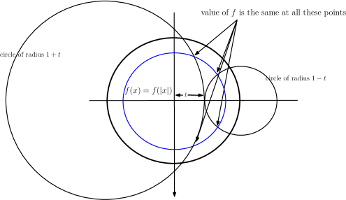
Figure 1. Relation between SMT of a radial function at radii $(1+t)$ and $(1-t)$ for $0<t<1$.

Notice that both the spheres (of radii $1\pm t$) pass through points having the same values of $f$. Let us consider the case of $3-$dimensions, where the necessary condition is straightforward to obtain. For $t\in(0,2)$, we have

$$\mathcal{R}f(t) =\frac{2\pi}{4\pi}\int\limits_{-1}^{1}f\left(\sqrt{1+t^{2}+2st}\right)\,\mathrm{d}s.$$

Consider the change of variables $u=\sqrt{1+t^{2}+2st}$ to obtain

$$\mathcal{R}f(t) =\frac{1}{2t}\int\limits_{|1-t|}^{1+t}uf(u)\,\mathrm{d}u$$

$$=\frac{1}{2t}\int\limits_{|1-t|}^{1}uf(u)\,\mathrm{d}u,$$

since $f$ vanishes outside the unit ball and it follows that the function $t\mathcal{R}f(t)$ satisfies

$$[t\mathcal{R}f](1-t) =[t\mathcal{R}f](1+t)\mbox{ for }t\in[0,1],$$

or equivalently

$$[t\mathcal{R}f](t) =[t\mathcal{R}f](2-t)\mbox{ for }t\in[0,1].$$

This relation also suggests working with $t^{n-2}\mathcal{R}f$ instead of $\mathcal{R}f$.

Let us move on to the proof of Theorem 1.1. We prove that the condition is necessary and sufficient in the next two subsections respectively.

3.1.1. Proof that the condition is necessary

In this subsection, we give the necessity part of the proof of the Theorem 1.1.

In order to see what condition to expect, let us consider the case of spherical Radon transform in 5-dimensions. Let $f$ be a smooth radial function supported in the unit ball in $\mathbb{R}^{5}$, that is, $f(x)=\widetilde{f}(|x|)$ for a smooth compactly supported function $\widetilde{f}$ on $[0,\infty)$. In order to avoid proliferation of new notation, we use the same $f$ to denote the function of one variable associated to $f$. That is, we denote $\widetilde{f}$ by $f$. We have

$$\mathcal{R}f(p,t)=\frac{1}{\omega_{5}}\int\limits_{\mathbb{S}^{4}}f(p+t\theta)\mathrm{d}\theta.$$ (3.1)

In (3.1) above, $\omega_{5}$ is the surface area of the unit sphere in $\mathbb{R}^{5}$. Then

$$g(t)=\mathcal{R}f(p,t) =\frac{1}{\omega_{5}}\int\limits_{\mathbb{S}^{4}}f(|p+t\theta|)\mathrm{d}\theta$$

$$=\frac{1}{\omega_{5}}\int\limits_{\mathbb{S}^{4}}f(\sqrt{1+t^{2}+2tp\cdot\theta})\mathrm{d}\theta.$$

Applying Funk-Hecke theorem, we get,

$$g(t)=\frac{\omega_{4}}{\omega_{5}}\int\limits_{t/2}^{1}f(\sqrt{1+t^{2}-2st})(1-s^{2})\mathrm{d}s.$$ (3.2)

For $t>0$, making the change of variable, $u=\sqrt{1+t^{2}-2st}$, we get,

$$g(t) =\frac{\omega_{4}}{t\omega_{5}}\int\limits_{|1-t|}^{1}f(u)u\left(1-\left(\frac{1+t^{2}-u^{2}}{2t}\right)^{2}\right)\mathrm{d}u$$

$$=\frac{\omega_{4}}{4t^{3}\omega_{5}}\int\limits_{|1-t|}^{1}f(u)u\left(4t^{2}-\left(1+t^{2}-u^{2}\right)^{2}\right)\mathrm{d}u.$$

Let us denote

$$h(t)=t^{3}g(t)\mbox{ and }C=\frac{\omega_{4}}{4\omega_{5}}.$$

Then we have

$$h(t) =C\int\limits_{|1-t|}^{1}f(u)u\left(4t^{2}-(1+t^{2}-u^{2})^{2}\right)\mathrm{d}u$$

$$=C\int\limits_{|1-t|}^{1}f(u)u\left((1+t)^{2}-u^{2}\right)(u^{2}-(t-1)^{2})\mathrm{d}u.$$

We let $0<t<1$. Then

$$h(t)=C\int\limits_{1-t}^{1}f(u)u\left((1+t)^{2}-u^{2}\right)(u^{2}-(t-1)^{2})\mathrm{d}u.$$ (3.3)

We replace $t$ by $2-t$ in the above expression. We get,

$$h(2-t)=C\int\limits_{1-t}^{1}f(u)u((3-t)^{2}-u^{2})(u^{2}-(t-1)^{2})\mathrm{d}u.$$ (3.4)

Let us expand both (3.3) and (3.4). Then

$$h(t)=-C(t^{2}-1)^{2}\int\limits_{1-t}^{1}f(u)u\mathrm{d}u+2C(1+t^{2})\int\limits_{1-t}^{1}f(u)u^{3}\mathrm{d}u-C\int\limits_{1-t}^{1}f(u)u^{5}\mathrm{d}u.$$ (3.5)

$$h(2-t)=-C((3-t)(1-t))^{2}\int\limits_{1-t}^{1}f(u)u\mathrm{d}u+2C(1+(2-t)^{2})\int\limits_{1-t}^{1}f(u)u^{3}\mathrm{d}u-C\int\limits_{1-t}^{1}f(u)u^{5}\mathrm{d}u.$$ (3.6)

For simplicity of notation, we will denote

$$\alpha=C\int\limits_{1-t}^{1}f(u)u\mathrm{d}u,\beta=C\int\limits_{1-t}^{1}f(u)u^{3}\mathrm{d}u,\gamma=C\int\limits_{1-t}^{1}f(u)u^{5}\mathrm{d}u.$$

Our goal is to find a relation eliminating these unknowns. In this notation, we have

$$h(t)=-(t^{2}-1)^{2}\alpha+2(1+t^{2})\beta-\gamma.$$ (3.7)

$$h(2-t)=-((3-t)(1-t))^{2}\alpha+2(1+(2-t)^{2})\beta-\gamma.$$ (3.8)

Differentiating the above two expressions, we get,

$$h^{\prime}(t)=-4t(t^{2}-1)\alpha+4t\beta.$$ (3.9)

$$h^{\prime}(2-t)=4(t-1)(t-2)(t-3)\alpha-4(t-2)\beta.$$ (3.10)

Note that those terms which involve the derivative of the integral add to $0$. Solving (3.9) and (3.10), we get,

$$\alpha=-\frac{(t-2)h^{\prime}(t)+th^{\prime}(2-t)}{16t(t-1)(t-2)}.$$ (3.11)

$$\beta=-\frac{(t-2)(t-3)h^{\prime}(t)+t(t+1)h^{\prime}(2-t)}{16t(t-2)}.$$ (3.12)

Substituting this back into (3.7) and (3.8), we then get (eliminating $\gamma$),

$$h(t)+(t^{2}-1)^{2}\alpha-2(1+t^{2})\beta=h(2-t)+((3-t)(1-t))^{2}\alpha-2(1+(2-t)^{2})\beta.$$

Using the expression for $\alpha$ and $\beta$, from (3.11) and (3.12), respectively, we have,

$$h(t)+\frac{(1-t)}{t}h^{\prime}(t)=h(2-t)+\frac{(1-t)}{(t-2)}h^{\prime}(2-t)\mbox{ for all }t\in(0,1).$$ (3.13)

In the notation of $D$ operator, we then get,

$$h(t)+(1-t)[Dh](t)=h(2-t)-(1-t)[Dh](2-t)\mbox{ for all }t\in(0,1).$$ (3.14)

By continuity, we also have

$$h(t)+(1-t)[Dh](t)=h(2-t)-(1-t)[Dh](2-t)\mbox{ for all }t\in[0,1].$$ (3.15)

This can be rewritten in the final form as follows:

$$h(t)-h(2-t)+(1-t)\left([Dh](t)+[Dh](2-t)\right)=0\mbox{ for all }t\in[0,1].$$ (3.16)

Note that due to the smoothness condition on $h$, the expression above is well-defined for $t=1$ as well.

Our goal next is to generalize the above approach for odd dimensional spherical Radon transform set-up. The strategy, as in this specific example, is to eliminate integral expressions involving $f$. We also make the following observations:

• We work with $D$ derivatives instead of the usual derivatives.

• In the general odd dimensional set-up, we can take up to $k^{\mathrm{th}}$ order $D$ derivatives and all such derivatives pass through the integral. In other words, the derivative of the integral has no contribution up to the $k^{\mathrm{th}}$ order.

• Based on the calculations done for the 5D-case, we consider coefficients of $D$ derivatives as powers of $(1-t)$ multiplied by suitable constants. As in (3.16), these are subtracted when evaluated at $t$ and $(2-t)$ for even order $D$ derivatives and added for odd order $D$ derivatives and set to $0$ to determine the coefficients.

We carry out this program for the general odd dimensional case now. We should mention here that while the computations done for the 5D case serve as a motivation for our approach below, it is very difficult to generalize it to higher dimensional cases, since the solution to the problem relies on the explicit inversion of a matrix. Nevertheless, finding the correct combination of derivatives leads to a positive answer as we show below. The 3D case is trivial, and the 5D computations done above can be recast as follows: Let us start with the expression for $h(t)$:

$$h(t) =\frac{\omega_{4}}{4\omega_{5}}\int\limits_{|1-t|}^{1}f(u)u\left(4t^{2}-(1+t^{2}-u^{2})^{2}\right)\mathrm{d}u$$

$$=\frac{\omega_{4}}{4\omega_{5}}\int\limits_{|1-t|}^{1}f(u)u\left(2(u^{2}+1)t^{2}-t^{4}-(1-u^{2})^{2}\right)\mathrm{d}u.$$

Let

$$P(t,u)=2(u^{2}+1)t^{2}-t^{4}-(1-u^{2})^{2}.$$

It is a straightforward exercise to check that

$$\left(P(t,u)-P(2-t,u)\right)+(1-t)\left([DP](t,u)+[DP](2-t,u)\right)\equiv 0.$$

This then gives that

$$\left(h(t)-h(2-t)\right)+(1-t)\left([Dh](t)+[Dh](2-t)\right)\equiv 0.$$

This is exactly what we derived earlier using a slightly different approach. Nevertheless, this serves as a motivation for what follows.

Proof of necessity of Theorem 1.1.

Let $n$ be of the form $n=2k+3$ with $k\geq 0$. Let $f\in C_{c}^{\infty}(\mathbb{B})$ in $n$ dimensions be a function depending only on the distance from the origin. Then $f$ can be written as

$$f(x)=\widetilde{f}(|x|),\mbox{ for some }\widetilde{f}:[0,\infty)\to\mathbb{R}.$$

We have that $\widetilde{f}\in C^{\infty}([0,\infty))$ and all odd order derivatives of $\widetilde{f}$ vanish at the origin. As before, we do not distinguish between $f$ and $\widetilde{f}$. The spherical Radon transform of $f$ is

$$\mathcal{R}f(p,t) =\frac{1}{\omega_{n}}\int\limits_{\mathbb{S}^{n-1}}f(|p+t\theta|)\mathrm{d}S(\theta)$$

$$=\frac{1}{\omega_{n}}\int\limits_{\mathbb{S}^{n-1}}f(\sqrt{1+t^{2}+2tp\cdot\theta})\mathrm{d}S(\theta)$$

$$=\frac{\omega_{n-1}}{\omega_{n}}\int\limits_{t/2}^{1}f(\sqrt{1+t^{2}-2ts})(1-s^{2})^{\frac{n-3}{2}}\mathrm{d}s.$$

The last equality follows from Funk-Hecke theorem combined with the fact that the support of $f$ is in the unit ball which forces $\frac{t}{2}\leq-p\cdot\theta\leq 1$. Next employing the change of variable,

$$1+t^{2}-2ts=u^{2},$$

we have

$$h(t):=t^{n-2}\mathcal{R}f(p,t) =\frac{\omega_{n-1}}{4^{k}\omega_{n}}\int\limits\limits_{|1-t|}^{1}uf(u)\left(4t^{2}-(1+t^{2}-u^{2})^{2}\right)^{k}\mathrm{d}u$$

$$=\frac{\omega_{n-1}}{4^{k}\omega_{n}}\int\limits\limits_{|1-t|}^{1}uf(u)\left(2(u^{2}+1)t^{2}-t^{4}-(1-u^{2})^{2}\right)^{k}\mathrm{d}u$$

The integral kernel for $h(t)$ is a polynomial in $t,u$ variables. In order to derive a necessary condition for a function $h(t)\in C_{c}^{\infty}((0,2))$ to be in the range of the spherical Radon transform, a reasonable approach would be differentiate $h$ several times and derive a system of equations eliminating integrals with integrand of the form $f(u)u^{m}$ for certain positive integers $m$. Before we proceed, we make the following remark. We are interested in taking $k$ derivatives of $h(t)$. In fact, $h$ is infinitely differentiable in $t$. This is clear for $t\neq 1$. However, for $t=1$, we can argue as follows. We have that $h(t)$ (involving the spherical Radon transform of a smooth function) is smooth in the $t$ variable and for $t\neq 1$, the derivatives of $h(t)$ can be computed by chain rule. Hence the derivatives of $h(t)$ at $t=1$ can be evaluated by taking the limit as $t\to 1$ of the corresponding derivatives evaluated at $t\neq 1$. The same remark applies for higher order $D$ derivatives instead of ordinary derivatives. With this remark in mind, we will not distinguish between $t=1$ and $t\neq 1$. With

$$Q(t,u)=2(u^{2}+1)t^{2}-t^{4}-(1-u^{2})^{2},$$

we consider $P(t,u)=\left(Q(t,u)\right)^{k}$, and we are interested in taking $D$ derivatives up to order $k$ of $h(t)$. Note that up to order $k$, the derivatives are only evaluated on $P(t,u)$, since $Q(t,1-t)=0$.

As a first step, we find explicit expression for higher order $D$ derivatives of $h(t)$. We use a special case of Faà di Bruno’s formula, Lemma 2.8: Let’s consider

$$P(t)=t^{k}\mbox{ and }Q(t,u)=2(u^{2}+1)t^{2}-t^{4}-(1-u^{2})^{2}.$$

In the set-up that we have, we take higher order $D$ derivatives of $Q$ and we observe that $D^{p}Q(t,u))=0$ for $p\geq 3$. Furthermore,

$$DQ(t,u)=4(u^{2}+1-t^{2})=4\left(\frac{Q(2-t,u)-Q(t,u)}{8(1-t)}+2(1-t)\right),$$

and

$$D^{2}Q(t,u)=-8.$$

With all these considerations, we arrive at the following formula for $D^{p}P(t,u)$:

$$D^{p}P(t,u)=\sum\limits_{q\geq p/2}^{p}\frac{k!}{(k-q)!}\left(Q(t,u)\right)^{k-q}\frac{p!}{(2q-p)!(p-q)!2^{p-q}}\left(\frac{Q(2-t,u)-Q(t,u)}{2(1-t)}+8(1-t)\right)^{2q-p}(-8)^{p-q}.$$

Let us write this as

$$D^{p}P(t,u) =\sum\limits_{q\geq p/2}^{p}\frac{K(p,q)}{(1-t)^{2q-p}}Q(t,u)^{k-q}(Q(2-t,u)-Q(t,u)+16(1-t)^{2})^{2q-p},$$ (3.17)

with

$$K(p,q)=\frac{k!p!(-4)^{p-q}}{(k-q)!(2q-p)!(p-q)!2^{2q-p}}.$$

Since we are only interested in derivatives in the $t$ variable, we are going to suppress the dependence of $P,Q$ and their derivatives on $u$, and simply write $P(t),Q(t)$, etc. We also recall our convention that $[D^{p}P](\cdot)$ denotes evaluation of the function $D^{p}P$ at the given point. Based on the necessary condition derived for the 5D case, keeping in mind odd or even order $D$ derivatives, let us consider

$$(1-t)^{p}\left([D^{p}P](t)+(-1)^{p+1}[D^{p}P](2-t)\right).$$ (3.18)

Let us expand $[D^{p}P](t)$ by binomial theorem. We get,

$$[D^{p}P](t) =\sum\limits_{q\geq p/2}^{p}\frac{K(p,q)}{(1-t)^{2q-p}}Q(t)^{k-q}\sum\limits_{r=0}^{2q-p}\binom{2q-p}{r}(Q(2-t)-Q(t))^{2q-p-r}16^{r}(1-t)^{2r}$$

$$=\sum\limits_{q\geq p/2}^{p}\sum\limits_{r=0}^{2q-p}\frac{16^{r}K(p,q)}{(1-t)^{2q-p}}(1-t)^{2r}\binom{2q-p}{r}Q(t)^{k-q}(Q(2-t)-Q(t))^{2q-p-r}.$$

Hence

$$[D^{p}P](2-t)\negthinspace=\negthinspace\negthinspace\negthinspace\negthinspace\sum\limits_{q\geq p/2}^{p}\sum\limits_{r=0}^{2q-p}\frac{(-1)^{2q-p-r}16^{r}K(p,q)}{(-1)^{2q-p}(1-t)^{2q-p}}(1-t)^{2r}\binom{2q-p}{r}Q(2-t)^{k-q}(Q(2-t)-Q(t))^{2q-p-r}.$$

Therefore

$$(1-t)^{p}\left([D^{p}P](t)+(-1)^{p+1}[D^{p}P](2-t)\right) =\sum\limits_{q\geq p/2}^{p}\sum\limits_{r=0}^{2q-p}K(p,q)16^{r}(1-t)^{2p-2q+2r}\binom{2q-p}{r}\times$$

$$(Q(2-t)-Q(t))^{2q-p-r}\Bigg{\{}Q(t)^{k-q}+(-1)^{p-r+1}Q(2-t)^{k-q}\Bigg{\}}.$$

We want to find coefficients $\{C(k,p)\}$ for $0\leq p\leq k$ such that

$$\sum\limits_{p=0}^{k}\sum\limits_{q\geq p/2}^{p}\sum\limits_{r=0}^{2q-p}C(k,p)K(p,q)(-1)^{2q-p-r}16^{r}(1-t)^{2p-2q+2r}{2q-p\choose r}\times$$

$$(Q(t)-Q(2-t))^{2q-p-r}\Bigg{\{}Q(t)^{k-q}+(-1)^{p-r+1}Q(2-t)^{k-q}\Bigg{\}}=0.$$

Simplifying the constants in the equality above, we arrive at

$$\sum\limits_{p=0}^{k}\sum\limits_{q\geq p/2}^{p}\sum\limits_{r=0}^{2q-p}C(k,p)\frac{k!p!(-1)^{q-r}2^{3p-4q+4r}}{(k-q)!(p-q)!r!(2q-p-r)!}(1-t)^{2(p-q+r)}$$ (3.19)

$$\times(Q(t)-Q(2-t))^{2q-p-r}\Big{\{}Q(t)^{k-q}+(-1)^{p-r+1}Q(2-t)^{k-q}\Big{\}}=0.$$

Our goal is to find constants $C(k,p)$ such that (3.19) is valid. Let us fix a power of $(1-t)^{2}$ of the form $(1-t)^{2(k-l)}$. Our strategy for determining the coefficients is to set sum of the terms corresponding to this fixed power $(1-t)^{2(k-l)}=0$. Let us assume $l$ is odd; the proof for the even case is similar. The maximum possible choices of triples $(p,q,r)$ we have to consider are:

1. $(k,k-l,k-2l),(k,k-l+1,k-2l+1),\cdots,(k,k,k-l)$

2. $(k-1,k-l,k-2l+1),(k-1,k-l+1,k-2l+2),\cdots,(k-1,k-1,k-l)$

3. $\vdots$

4. $(k-l,k-l,k-l)$.

The maximum number of terms above is $\frac{(l+1)(l+2)}{2}$.

We prove our result by induction. Let us start by considering the highest power of $(1-t)$ in (3.19).

We claim that a term of the form $(1-t)^{2k}$ does not appear in the expansion above. This can be seen as follows: To get the term, $(1-t)^{2(p-q+r)}=(1-t)^{2k}$, we must have $p-q+r=k$. If $p<k$, then we must have $q<r$. But we have $0\leq r\leq 2q-p<2r-p$. This then implies that $r<2r-p$, which then gives that $r>p$, but this impossible. Hence $p=k$. This then gives $r=q$, which then gives that $p\leq q$. But $q\leq p$ always and hence $q=p=k$. This forces $r=k$. Due to the presence of $(-1)^{p-r+1}$ in the term above, we get that $(1-t)^{2k}$ term does not appear in the expansion above.

Next we show that a term involving $(1-t)^{2k-2}$ appears exactly twice in the term involving $C(k,k)$ and once in the term involving $C(k,k-1)$. First, consider $p=k$. Then we have to consider $p-q+r=k-1$, and since $p=k$, we have $q-r=1$, which then implies that $k-1\leq q$. Hence the two choices of $q$ that are possible are $q=k-1$ and $q=k$. If $q=k-1$, then $r=k-2$, and if $q=k$, then $r=k-1$. If we consider $p=k-1$, then exactly the same argument as in the previous paragraph leads to $r=q=p=k-1$. Hence only one choice is possible. Next let $p=k-2$. We then have $r-q=1$, and following the same arguments as above, we get that $q\geq k-1$, which is impossible since $q\leq p=k-2$. A similar argument follows for all $p<k-2$. Hence we have established that there are exactly three terms.

Summarizing the content of the above paragraph, there are exactly 3 terms in the above expansion involving $(1-t)^{2k-2}$. They correspond to the following triples: $(p,q,r)=(k,k-1,k-2),(k,k,k-1)$ and $(k-1,k-1,k-1)$. We have to be careful with terms involving the case when $q=k$, since in this case, $Q(t)^{k-q}+(-1)^{p-r+1}Q(2-t)^{k-q}$ is either $0$ or $2$. Note that this appears below when dealing with $K(k,k)$ term. Setting the term involving $(1-t)^{2k-2}$ to be $0$, we get

$$\Bigg{\{}C(k,k)\Bigg{\{}K(k,k-1)8^{k-2}-K(k,k)8^{k-1}k\Bigg{\}}+C(k,k-1)K(k-1,k-1)8^{k-1}\Bigg{\}}(Q(t)-Q(2-t))=0.$$

By setting the terms within the outer parantheses to be $0$ and using the values of $K(k,k-1),K(k,k)$ and $K(k-1,k-1)$, we then get the following:

$$-C(k,k)\Bigg{\{}\frac{4k!^{2}8^{k-2}}{(k-2)!}+k!8^{k-1}k\Bigg{\}}+C(k,k-1)k!8^{k-1}=0.$$ (3.20)

Setting $C(k,k)=1$, we find that $C(k,k-1)=k(k+1)/2$. Notice that the values of $\{C(k,p)\}$ are unique up to a normalizing constant. We choose the normalization so that $C(k,k)=1$.

Let us assume by induction that $C(k,k-s)=\frac{(k+s)!}{(k-s)!2^{s}s!}$ for all $0\leq s\leq l-1$. Note that $C(k,k)=1$. Our goal is to determine $C(k,k-l)$. For ease of notation, from now on, we let $A=Q(t)$ and $B=Q(2-t)$.

The terms corresponding to the triples from (1) above are:

$$-C(k,k)(k!)^{2}2^{3k-4l}\sum\limits_{s=0}^{l}\frac{(A-B)^{s}\left(A^{l-s}+(-1)^{2l+1-s}B^{l-s}\right)}{((l-s)!)^{2}(k-2l+s)!s!}.$$

The terms corresponding to the triples $(p,q,r)$ from (2) above are:

$$C(k,k-1)k!(k-1)!2^{3k-4l+1}\sum\limits_{s=0}^{l-1}\frac{(A-B)^{s}(A^{l-s}+(-1)^{2l-s-1}B^{l-s})}{(l-s)!(l-s-1)!(k-2l+1+s)!s!}.$$

The terms corresponding to triples $(p,q,r)$ with $p=k-2$ are:

$$-C(k,k-2)k!(k-2)!2^{3k-4l+2}\sum\limits_{s=0}^{l-2}\frac{(A-B)^{s}(A^{l-s}+(-1)^{2l-s-3}B^{l-s})}{(l-s)!(l-s-2)!(k-2l+2+s)!s!}.$$

Continuing in this fashion and summing up all the terms corresponding to $(1-t)^{2(k-l)}$ and setting it to $0$, we have

$$k!\sum\limits_{m=0}^{l}(-1)^{l-m}C(k,k-m)(k-m)!2^{3k-4l+m}\sum\limits_{s=0}^{l-m}\frac{(A-B)^{s}(A^{l-s}-(-1)^{2l-s}B^{l-s})}{(l-s)!(l-s-m)!(k-2l+s+m)!s!}=0.$$

We ignore $k!$ and $2^{3k-4l}$ in the above expression from now on. Interchanging the order of summation, we get,

$$\sum\limits_{s=0}^{l}\sum\limits_{m=0}^{l-s}(-1)^{l-m}C(k,k-m)(k-m)!2^{m}\frac{(A-B)^{s}(A^{l-s}-(-1)^{s}B^{l-s})}{(l-s)!(l-s-m)!(k-2l+s+m)!s!}=0.$$ (3.21)

Let us split (3.21) as

$$\sum\limits_{s=1}^{l-1}\sum\limits_{m=1}^{l-s}(-1)^{l-m}C(k,k-m)(k-m)!2^{m}\frac{(A-B)^{s}(A^{l-s}-(-1)^{s}B^{l-s})}{(l-s)!(l-s-m)!(k-2l+s+m)!s!}$$

$$+\sum\limits_{m=1}^{l-1}\frac{(-1)^{l-m}C(k,k-m)(k-m)!2^{m}(A^{l}-B^{l})}{l!(l-m)!(k-2l+m)!}-2(A-B)^{l}{k\choose l}$$

$$-\sum\limits_{s=1}^{l-1}\frac{k!(A-B)^{s}(A^{l-s}-(-1)^{s}B^{l-s})}{((l-s)!)^{2}(k-2l+s)!s!}+\frac{C(k,k-l)2^{l}(A^{l}-B^{l})}{l!}-\frac{k!(A^{l}-B^{l})}{(l!)^{2}(k-2l)!}=0.$$

Using the fact that $C(k,k-m)=\frac{(k+m)!}{(k-m)!2^{m}m!}$ for $0\leq m<l$, we get,

$$\sum\limits_{s=1}^{l-1}\sum\limits_{m=1}^{l-s}(-1)^{l-m}\frac{(k+m)!(A-B)^{s}(A^{l-s}-(-1)^{s}B^{l-s})}{m!(l-s)!(l-s-m)!(k-2l+s+m)!s!}-\sum\limits_{m=1}^{l-1}(-1)^{m}\frac{(k+m)!(A^{l}-B^{l})}{l!m!(l-m)!(k-2l+m)!}$$

$$-2(A-B)^{l}{k\choose l}-\sum\limits_{s=1}^{l-1}\frac{k!(A-B)^{s}(A^{l-s}-(-1)^{s}B^{l-s})}{((l-s)!)^{2}(k-2l+s)!s!}+\frac{C(k,k-l)2^{l}(A^{l}-B^{l})}{l!}-\frac{k!(A^{l}-B^{l})}{(l!)^{2}(k-2l)!}=0.$$

We can write this as

$$-\sum\limits_{s=1}^{l-1}\frac{(2l-s)!(A-B)^{s}(A^{l-s}-(-1)^{s}B^{l-s})}{((l-s)!)^{2}s!}\sum\limits_{m=1}^{l-s}(-1)^{m}{k+m\choose 2l-s}{l-s\choose m}$$ (3.22)

$$-\frac{(2l)!(A^{l}-B^{l})}{(l!)^{2}}\sum\limits_{m=1}^{l-1}(-1)^{m}{k+m\choose 2l}{l\choose m}-2(A-B)^{l}{k\choose l}$$

$$-\sum\limits_{s=1}^{l-1}{k\choose 2l-s}{2l-s\choose l}{l\choose s}(A-B)^{s}(A^{l-s}-(-1)^{s}B^{l-s})$$

$$+\frac{C(k,k-l)2^{l}(A^{l}-B^{l})}{l!}-\frac{k!(A^{l}-B^{l})}{(l!)^{2}(k-2l)!}=0.$$

Our next step is to simplify the first summand in (3.22) above, which we denote by $\beta$:

$$\beta=-\sum\limits_{s=1}^{l-1}\frac{(2l-s)!(A-B)^{s}(A^{l-s}-(-1)^{s}B^{l-s})}{((l-s)!)^{2}s!}\sum\limits_{m=1}^{l-s}(-1)^{m}{k+m\choose 2l-s}{l-s\choose m}.$$

We first simplify the second summand in $\beta$: We write using Vandermonde identity [27]:

$${k+m\choose 2l-s}=\sum\limits_{j=1}^{m}{k\choose 2l-s-j}{m\choose j}+{k\choose 2l-s},$$

the second term on the right being the term corresponding to the index $j=0$ from the first sum. Using this, we have,

$$\sum\limits_{m=1}^{l-s}(-1)^{m}{k+m\choose 2l-s}{l-s\choose m} \negthinspace\negthinspace=\negthinspace\negthinspace\sum\limits_{m=1}^{l-s}(-1)^{m}\Bigg{\{}\sum\limits_{j=1}^{m}{k\choose 2l-s-j}{m\choose j}+{k\choose 2l-s}\Bigg{\}}{l-s\choose m}$$

$$\negthinspace\negthinspace=\negthinspace\negthinspace\sum\limits_{m=1}^{l-s}(-1)^{m}\Bigg{\{}\sum\limits_{j=1}^{m}{k\choose 2l-s-j}{m\choose j}{l-s\choose m}+{k\choose 2l-s}{l-s\choose m}\Bigg{\}}$$

$$\negthinspace\negthinspace=\negthinspace\negthinspace\sum\limits_{m=1}^{l-s}(-1)^{m}\Bigg{\{}\sum\limits_{j=1}^{m}{k\choose 2l-s-j}{l-s\choose j}{l-s-j\choose l-s-m}+{k\choose 2l-s}{l-s\choose m}\Bigg{\}}.$$

In the last equality, we have used the standard fact:

$${a\choose b}{b\choose c}={a\choose c}{a-c\choose b-c}={a\choose c}{a-c\choose a-b}.$$

Let us interchange the order of summation. We then get,

$$\sum\limits_{m=1}^{l-s}(-1)^{m}{k+m\choose 2l-s}{l-s\choose m} =\sum\limits_{j=1}^{l-s}\sum\limits_{m=j}^{l-s}(-1)^{m}{k\choose 2l-s-j}{l-s\choose j}{l-s-j\choose l-s-m}$$ (3.23)

$$+\sum\limits_{m=1}^{l-s}(-1)^{m}{k\choose 2l-s}{l-s\choose m}.$$ (3.24)

Note that

$$\sum\limits_{m=0}^{l-s}(-1)^{m}{l-s\choose m}=0.$$

Hence (3.24) simplifies to

$$\sum\limits_{m=1}^{l-s}(-1)^{m}{k\choose 2l-s}{l-s\choose m}=-{k\choose 2l-s}.$$

Next let us consider the first summand on the right in (3.23). We write

$$\sum\limits_{j=1}^{l-s}\sum\limits_{m=j}^{l-s}(-1)^{m}{k\choose 2l-s-j}{l-s\choose j}{l-s-j\choose l-s-m}$$

$$=\sum\limits_{j=1}^{l-s-1}\sum\limits_{m=j}^{l-s}(-1)^{m}{k\choose 2l-s-j}{l-s\choose j}{l-s-j\choose l-s-m}+(-1)^{l-s}{k\choose l}$$

$$=\sum\limits_{j=1}^{l-s-1}{k\choose 2l-s-j}{l-s\choose j}\sum\limits_{m=j}^{l-s}(-1)^{m}{l-s-j\choose l-s-m}+(-1)^{l-s}{k\choose l}.$$

We have that

$$\sum\limits_{m=j}^{l-s}(-1)^{m}{l-s-j\choose l-s-m}=0.$$

Hence

$$\sum\limits_{j=1}^{l-s}\sum\limits_{m=j}^{l-s}(-1)^{m}{k\choose 2l-s-j}{l-s\choose j}{l-s-j\choose l-s-m}=(-1)^{l-s}{k\choose l}.$$

Putting this together, we get

$$\sum\limits_{m=1}^{l-s}(-1)^{m}{k+m\choose 2l-s}{l-s\choose m} =(-1)^{l-s}{k\choose l}-{k\choose 2l-s}.$$ (3.25)

Substituting (3.25) into $\beta$, we have

$$\beta =-{k\choose l}\sum\limits_{s=1}^{l-1}(-1)^{l-s}\frac{(2l-s)!(A-B)^{s}(A^{l-s}-(-1)^{s}B^{l-s})}{((l-s)!)^{2}s!}$$

$$+\sum\limits_{s=1}^{l-1}{k\choose 2l-s}\frac{(2l-s)!(A-B)^{s}(A^{l-s}-(-1)^{s}B^{l-s})}{((l-s)!)^{2}s!}$$

We write

$$\frac{(2l-s)!}{((l-s)!)^{2}s!}={2l-s\choose l-s}{l\choose s}={2l-s\choose l}{l\choose s}.$$

With this, we have

$$\beta =-{k\choose l}\sum\limits_{s=1}^{l-1}(-1)^{l-s}{2l-s\choose l}{l\choose s}(A-B)^{s}(A^{l-s}-(-1)^{s}B^{l-s})$$

$$+\sum\limits_{s=1}^{l-1}{k\choose 2l-s}{2l-s\choose l}{l\choose s}(A-B)^{s}(A^{l-s}-(-1)^{s}B^{l-s})$$

$$={k\choose l}\sum\limits_{s=1}^{l-1}(-1)^{s}{2l-s\choose l}{l\choose s}(A-B)^{s}(A^{l-s}-(-1)^{s}B^{l-s})$$

$$+{k\choose l}\sum\limits_{s=1}^{l-1}{k-l\choose l-s}{l\choose s}(A-B)^{s}(A^{l-s}-(-1)^{s}B^{l-s}).$$

Note that in the second line from bottom above, we have used the fact that $l$ is odd. Let us write

$${k\choose l}\sum\limits_{s=1}^{l-1}(-1)^{s}{2l-s\choose l}{l\choose s}(A-B)^{s}(A^{l-s}-(-1)^{s}B^{l-s})$$

$$={k\choose l}\Bigg{\{}\sum\limits_{s=0}^{l}(-1)^{s}{2l-s\choose l}{l\choose s}(A-B)^{s}(A^{l-s}-(-1)^{s}B^{l-s})-\frac{(2l)!}{(l!)^{2}}(A^{l}-B^{l})+2(A-B)^{l}\Bigg{\}}.$$

Hence

$$\beta ={k\choose l}\Bigg{\{}\sum\limits_{s=0}^{l}(-1)^{s}{2l-s\choose l}{l\choose s}(A-B)^{s}(A^{l-s}-(-1)^{s}B^{l-s})-\frac{(2l)!}{(l!)^{2}}(A^{l}-B^{l})+2(A-B)^{l}\Bigg{\}}$$

$$+{k\choose l}\sum\limits_{s=1}^{l-1}{k-l\choose l-s}{l\choose s}(A-B)^{s}(A^{l-s}-(-1)^{s}B^{l-s}).$$

Lemma 3.1.

We have that for any $A$ and $B$ and for any $l\geq 0$,

$$\sum\limits_{s=0}^{l}(-1)^{s}{2l-s\choose l}{l\choose s}(A-B)^{s}(A^{l-s}-(-1)^{s}B^{l-s})=0.$$

Proof.

We first split the left hand side as follows:

$$\sum\limits_{s=0}^{l}(-1)^{s}{2l-s\choose l}{l\choose s}(A-B)^{s}(A^{l-s}-(-1)^{s}B^{l-s}) =\sum\limits_{s=0}^{l}{2l-s\choose l}{l\choose s}(B-A)^{s}A^{l-s}$$

$$-\sum\limits_{s=0}^{l}{2l-s\choose l}{l\choose s}(A-B)^{s}B^{l-s}.$$

Here and in several instances throughout the rest of the paper, we use contour integration technique to evaluate combinatorial sums pioneered by Egorychev [22]. We write

$${2l-s\choose l}=\frac{1}{2\pi\mathrm{i}}\int\limits_{|z|=\varepsilon}\frac{(1+z)^{2l-s}}{z^{l+1}}\mathrm{d}z,$$

and hence

$$\sum\limits_{s=0}^{l}{2l-s\choose l}{l\choose s}(B-A)^{s}A^{l-s} =\frac{1}{2\pi\mathrm{i}}\int\limits_{|z|=\varepsilon}\sum\limits_{s=0}^{l}{l\choose s}(B-A)^{s}A^{l-s}\frac{(1+z)^{2l-s}}{z^{l+1}}\mathrm{d}z$$

$$=\frac{1}{2\pi\mathrm{i}}\int\limits_{|z|=\varepsilon}\sum\limits_{s=0}^{l}{l\choose s}\left(\frac{B-A}{1+z}\right)^{s}A^{l-s}\frac{(1+z)^{2l}}{z^{l+1}}\mathrm{d}z$$

$$=\frac{1}{2\pi\mathrm{i}}\int\limits_{|z|=\varepsilon}\left(A+\frac{B-A}{1+z}\right)^{l}\frac{(1+z)^{2l}}{z^{l+1}}\mathrm{d}z$$

$$=\frac{1}{2\pi\mathrm{i}}\int\limits_{|z|=\varepsilon}\frac{((B+Az)(1+z))^{l}}{z^{l+1}}\mathrm{d}z.$$

Similarly,

$$\sum\limits_{s=0}^{l}{2l-s\choose l}{l\choose s}(A-B)^{s}B^{l-s}=\frac{1}{2\pi\mathrm{i}}\int\limits_{|z|=\varepsilon}\frac{((A+Bz)(1+z))^{l}}{z^{l+1}}\mathrm{d}z.$$

We would like to show then that

$$\frac{1}{2\pi\mathrm{i}}\int\limits_{|z|=\varepsilon}\frac{((B+Az)(1+z))^{l}}{z^{l+1}}\mathrm{d}z-\frac{1}{2\pi\mathrm{i}}\int\limits_{|z|=\varepsilon}\frac{((A+Bz)(1+z))^{l}}{z^{l+1}}\mathrm{d}z=0.$$

Expanding $(B+Az)^{l}(1+z)^{l}$ using binomial theorem, we get,

$$(B+Az)^{l}(1+z)^{l}=\sum\limits_{u,v=0}^{l}{l\choose u}{l\choose v}B^{u}A^{l-u}z^{l-u}z^{v}.$$

Then

$$\frac{(B+Az)^{l}(1+z)^{l}}{z^{l+1}}=\frac{\sum\limits_{u,v=0}^{l}{l\choose u}{l\choose v}B^{u}A^{l-u}z^{v-u}}{z}.$$

Hence

$$\frac{1}{2\pi\mathrm{i}}\int\limits_{|z|=\varepsilon}\frac{((B+Az)(1+z))^{l}}{z^{l+1}}\mathrm{d}z=\sum\limits_{u=0}^{l}{l\choose u}^{2}B^{u}A^{l-u},$$

by Cauchy’s theorem combined with the fact that for any negative power of $z$ that is not $-1$, the integral vanishes, since $z^{-p}$ has a primitive in a neighborhood of $|z|=\varepsilon$ for $p\neq 1$. Similarly,

$$\frac{(A+Bz)^{l}(1+z)^{l}}{z^{l+1}}=\frac{\sum\limits_{u,v=0}^{l}{l\choose u}{l\choose v}A^{u}B^{l-u}z^{v-u}}{z}.$$

Exactly the same argument gives,

$$\frac{1}{2\pi\mathrm{i}}\int\limits_{|z|=\varepsilon}\frac{(A+Bz)^{l}(1+z)^{l}}{z^{l+1}}\mathrm{d}z=\sum\limits_{u=0}^{l}{l\choose u}^{2}A^{u}B^{l-u}.$$

Since ${l\choose u}={l\choose l-u}$, these two sums are the same. This concludes the proof of the lemma. ∎

Going back to the proof of the result, we have now

$$\beta ={k\choose l}\Bigg{\{}-\frac{(2l)!}{(l!)^{2}}(A^{l}-B^{l})+2(A-B)^{l}\Bigg{\}}+{k\choose l}\sum\limits_{s=1}^{l-1}{k-l\choose l-s}{l\choose s}(A-B)^{s}(A^{l-s}-(-1)^{s}B^{l-s}).$$

Substituting this into (3.22), we then get,

$$0 ={k\choose l}\Bigg{\{}-\frac{(2l)!}{(l!)^{2}}(A^{l}-B^{l})+2(A-B)^{l}\Bigg{\}}+{k\choose l}\sum\limits_{s=1}^{l-1}{k-l\choose l-s}{l\choose s}(A-B)^{s}(A^{l-s}-(-1)^{s}B^{l-s})$$ (3.26)

$$-\frac{(2l)!(A^{l}-B^{l})}{(l!)^{2}}\sum\limits_{m=1}^{l-1}(-1)^{m}{k+m\choose 2l}{l\choose m}-2(A-B)^{l}{k\choose l}$$

$$-\sum\limits_{s=1}^{l-1}{k\choose 2l-s}{2l-s\choose l}{l\choose s}(A-B)^{s}(A^{l-s}-(-1)^{s}B^{l-s})+\frac{C(k,k-l)2^{l}(A^{l}-B^{l})}{l!}-\frac{k!(A^{l}-B^{l})}{(l!)^{2}(k-2l)!}.$$

Finally, let us simplify the third summand on the right:

$$\sum\limits_{m=1}^{l-1}(-1)^{m}{k+m\choose 2l}{l\choose m}.$$

We have, again using Vandermonde identity,

$$\sum\limits_{m=1}^{l-1}(-1)^{m}{k+m\choose 2l}{l\choose m}=\sum\limits_{m=1}^{l-1}(-1)^{m}\sum\limits_{j=1}^{m}{k\choose 2l-j}{m\choose j}{l\choose m}+\sum\limits_{m=1}^{l-1}(-1)^{m}{k\choose 2l}{l\choose m}.$$

We note that in the second sum above, there are at least two terms in the expansion since $m$ starts from $1$ and $l$ is odd. Hence the second summand on the right is $0$. Then

$$\sum\limits_{m=1}^{l-1}(-1)^{m}{k+m\choose 2l}{l\choose m}=\sum\limits_{m=1}^{l-1}(-1)^{m}\sum\limits_{j=1}^{m}{k\choose 2l-j}{l\choose j}{l-j\choose m-j}.$$

Interchanging the order of summation, we get,

$$\sum\limits_{m=1}^{l-1}(-1)^{m}{k+m\choose 2l}{l\choose m} =\sum\limits_{j=1}^{l-1}{k\choose 2l-j}{l\choose j}\sum\limits_{m=j}^{l-1}(-1)^{m}{l-j\choose m-j}$$

$$=\sum\limits_{j=1}^{l-1}{k\choose 2l-j}{l\choose j}.$$

Note that the second line follows due to the fact that

$$0 =\sum\limits_{m=j}^{l}(-1)^{m}{l-j\choose m-j}$$

$$=\sum\limits_{m=j}^{l-1}(-1)^{m}{l-j\choose m-j}+(-1)^{l}.$$

Since $l$ is assumed to be odd, we get,

$$\sum\limits_{m=j}^{l-1}(-1)^{m}{l-j\choose m-j}=1.$$

We have,

$$\sum\limits_{k}{p\choose k}{q-j\choose q-k}={p+q-j\choose q}.$$

Using this formula, we get,

$$\sum\limits_{m=1}^{l-1}(-1)^{m}{k+m\choose 2l}{l\choose m}={k+l\choose 2l}-{k\choose 2l}-{k\choose l}.$$

Using this in (3.26), we have

$$0 ={k\choose l}\Bigg{\{}-\frac{(2l)!}{(l!)^{2}}(A^{l}-B^{l})+2(A-B)^{l}\Bigg{\}}+{k\choose l}\sum\limits_{s=1}^{l-1}{k-l\choose l-s}{l\choose s}(A-B)^{s}(A^{l-s}-(-1)^{s}B^{l-s})$$ (3.27)

$$-\frac{(2l)!(A^{l}-B^{l})}{(l!)^{2}}\Bigg{\{}{k+l\choose 2l}-{k\choose 2l}-{k\choose l}\Bigg{\}}$$

$$-2(A-B)^{l}{k\choose l}-\sum\limits_{s=1}^{l-1}{k\choose 2l-s}{2l-s\choose l}{l\choose s}(A-B)^{s}(A^{l-s}-(-1)^{s}B^{l-s})$$

$$+\frac{C(k,k-l)2^{l}(A^{l}-B^{l})}{l!}-\frac{k!(A^{l}-B^{l})}{(l!)^{2}(k-2l)!}.$$

The second and fifth terms on the right in (3.27) cancel. Further cancelling out other common terms in (3.27), we arrive at

$$C(k,k-l)=\frac{(k+l)!}{(k-l)!2^{l}l!}.$$

This completes the induction step. A similar argument can be employed for the case of $l$ even and for this reason we will skip the proof.

Going back to (3.19), we have found the coefficients $C(k,p)$ such that this equation is $0$. In other words, we have obtained the following:

$$\sum\limits_{p=0}^{k}C(k,p)(1-t)^{p}\left([D^{p}P](t)+(-1)^{p+1}[D^{p}P](2-t)\right)=0,$$

where

$$C(k,p)=\frac{(2k-p)!}{p!2^{k-p}(k-p)!}.$$

Since, as already mentioned above, the $D$ derivatives up to order $k$ of $h(t)$ are applied only to $P(t,u)$, we have obtained the following necessary condition for a function $g\in C_{c}^{\infty}((0,2))$ to be in the range of a smooth radial function supported in the unit ball in $\mathbb{R}^{n}$, where $n=2k+3$: Letting $h(t)=t^{n-2}g(t)$, we have for all $t\in[0,1]$

$$\Bigg{\{}\sum\limits_{p=0}^{k}C(k,p)(1-\cdot)^{p}[D^{p}h(\cdot)]\Bigg{\}}(t)=\Bigg{\{}\sum\limits_{p=0}^{k}C(k,p)(1-\cdot)^{p}[D^{p}h(\cdot)]\Bigg{\}}(2-t).$$ (3.28)

∎

3.1.2. Proof of sufficiency in Theorem 1.1

In this subsection, we give the proof of sufficiency of Theorem 1.1. We start with a result about special functions that could be of independent interest.

Theorem 3.2.

Let $h(t)\in C_{c}^{\infty}((0,2))$ satisfy the following evenness condition:

$$\Bigg{\{}\sum\limits_{p=0}^{k}C(k,p)(1-\cdot)^{p}[D^{p}h](\cdot)\Bigg{\}}(1-t)=\Bigg{\{}\sum\limits_{p=0}^{k}C(k,p)(1-\cdot)^{p}[D^{p}h](\cdot)\Bigg{\}}(1+t)\mbox{ for all }t\in[0,1].$$ (3.29)

Then $h(t)$ satisfies the following identity: For $\lambda>0$:

$$\left(\int\limits_{0}^{\infty}j_{k+\tfrac{1}{2}}(\lambda t)th(t)\mathrm{d}t\right)y_{k+\tfrac{1}{2}}(\lambda)=\left(\int\limits_{0}^{\infty}y_{k+\tfrac{1}{2}}(\lambda t)th(t)\mathrm{d}t\right)j_{k+\tfrac{1}{2}}(\lambda).$$ (3.30)

Proof.

We define

$$H(t) =\sum\limits_{p=0}^{k}C(k,p)(1-t)^{p}[D^{p}h](t).$$

We observe the following properties of $H(t)$.

1. $H(t)=H(2-t)$ for $0\leq t\leq 1$,

2. $H(t)=0$ for $t>2$.

We claim that the following integral

$$I_{k}=\int\limits_{0}^{\infty}\sum\limits_{p=0}^{k}C(k,p)(1-t)^{p}[D^{p}h](t)j_{k+\frac{1}{2}}(\lambda(t-1))(t-1)\mathrm{d}t=0.$$ (3.31)

To see this, first of all, we observe that due to the support condition on $h$, $H(t)$ has non-trivial support only in $(0,2)$. Then

$$I_{k} =\int\limits_{0}^{2}\sum\limits_{p=0}^{k}C(k,p)(1-t)^{p}[D^{p}h](t)j_{k+\tfrac{1}{2}}(\lambda(t-1))(t-1)\mathrm{d}t$$

$$=\int\limits_{0}^{1}\sum\limits_{p=0}^{k}C(k,p)(1-t)^{p}[D^{p}h](t)j_{k+\tfrac{1}{2}}(\lambda(t-1))(t-1)\mathrm{d}t$$

$$+\int\limits_{1}^{2}\sum\limits_{p=0}^{k}C(k,p)(1-t)^{p}[D^{p}h](t)j_{k+\tfrac{1}{2}}(\lambda(t-1))(t-1)\mathrm{d}t.$$

Substituting $t$ by $2-t$ in the second integral, noting that $j_{k+\tfrac{1}{2}}(x)$ is an even function in $x$, and using (3.29), we have

$$I_{k} =\int\limits_{0}^{1}\sum\limits_{p=0}^{k}C(k,p)(1-t)^{p}[D^{p}h](t)j_{k+\tfrac{1}{2}}(\lambda(t-1))(t-1)\mathrm{d}t$$

$$-\int\limits_{0}^{1}\sum\limits_{p=0}^{k}C(k,p)(1-t)^{p}[D^{p}h](t)j_{k+\frac{1}{2}}(\lambda(t-1))(t-1)\mathrm{d}t=0.$$

Next we have

$$0 =I_{k}=\int\limits_{0}^{\infty}\sum\limits_{p=0}^{k}C(k,p)(1-t)^{p}[D^{p}h](t)j_{k+\frac{1}{2}}(\lambda(t-1))(t-1)\mathrm{d}t$$

$$=\int\limits_{0}^{\infty}\sum\limits_{p=0}^{k}C(k,p)th(t)D^{p}\left(\frac{(t-1)^{p+1}j_{k+\frac{1}{2}}(\lambda(t-1))}{t}\right)\mathrm{d}t.$$

Substituting $t$ by $-t$, we get

$$I_{k} =-\int\limits_{-\infty}^{0}\sum\limits_{p=0}^{k}(-1)^{p}C(k,p)D^{p}\left(\frac{(t+1)^{p+1}j_{k+\frac{1}{2}}(\lambda(t+1))}{t}\right)th(-t)\mathrm{d}t.$$

From Theorem 3.3 below, we obtain the following equality. This is a technical result and in order not to disturb the flow of proof, we prefer to give it at the end.

$$I_{k}=(-1)^{k+1}\int\limits_{-\infty}^{0}\left\{D^{k}\left(\frac{\sin(\lambda t)}{t}\right)y_{k+\tfrac{1}{2}}({\lambda})+D^{k}\left(\frac{\cos(\lambda t)}{t}\right)j_{k+\tfrac{1}{2}}({\lambda})\right\}th(-t)\mathrm{d}t.$$

From the formulas in Lemma 3.4, we see that

$$D^{k}\left(\frac{\sin\lambda(\cdot)}{(\cdot)}\right)(-t)=D^{k}\left(\frac{\sin\lambda(\cdot)}{(\cdot)}\right)(t),$$

$$D^{k}\left(\frac{\cos\lambda(\cdot)}{(\cdot)}\right)(-t)=-D^{k}\left(\frac{\cos\lambda(\cdot)}{(\cdot)}\right)(t).$$

Letting $t\to-t$ in the integral above, we have

$$0=(-1)^{k}\int\limits_{0}^{\infty}\left\{D^{k}\left(\frac{\sin(\lambda t)}{t}\right)y_{k+\tfrac{1}{2}}({\lambda})-D^{k}\left(\frac{\cos(\lambda t)}{t}\right)j_{k+\tfrac{1}{2}}({\lambda})\right\}th(t)\mathrm{d}t.$$

Hence

$$\left(\int\limits_{0}^{\infty}D^{k}\left(\frac{\sin(\lambda t)}{t}\right)th(t)\mathrm{d}t\right)y_{k+\tfrac{1}{2}}(\lambda)=\left(\int\limits_{0}^{\infty}D^{k}\left(\frac{\cos(\lambda t)}{t}\right)\,th((t)\mathrm{d}t\right)j_{k+\tfrac{1}{2}}(\lambda).$$ (3.32)

The above formula (3.32) can be written in a more symmetric form as follows. For $\lambda>0$:

$$\left(\int\limits_{0}^{\infty}j_{k+\tfrac{1}{2}}(\lambda t)th(t)\mathrm{d}t\right)y_{k+\tfrac{1}{2}}(\lambda)=\left(\int\limits_{0}^{\infty}y_{k+\tfrac{1}{2}}(\lambda t)th(t)\mathrm{d}t\right)j_{k+\tfrac{1}{2}}(\lambda).$$

∎

Theorem 3.3.

Let $j_{k+1/2}(x)=D^{k}\left(\frac{\sin x}{x}\right)$ be the spherical Bessel function of the first kind modulo constants and recall $C(k,p)=\frac{(2k-p)!}{p!(k-p)!2^{k-p}}$. For $\lambda>0$ and $t\neq 0$,

$$M_{k}(\lambda) :=\sum\limits_{p=0}^{k}C(k,p)(-1)^{p}D^{p}\left(\frac{(1+t)^{p+1}j_{k+\tfrac{1}{2}}(\lambda(1+t))}{t}\right)$$ (3.33)

$$=(-1)^{k}\left\{D^{k}\left(\frac{\sin(\lambda t)}{t}\right)y_{k+\tfrac{1}{2}}({\lambda})+D^{k}\left(\frac{\cos(\lambda t)}{t}\right)j_{k+\tfrac{1}{2}}({\lambda})\right\},$$

where

$$y_{k+\tfrac{1}{2}}(x)=D^{k}\left(\frac{\cos x}{x}\right),$$

is the spherical Bessel function of the second kind modulo constants.

We collect a few formulas first:

Lemma 3.4.

We have

$$D^{p}\left(\frac{\sin x}{x}\right)=\sum_{l=0}^{p}\frac{C(p,l)x^{l}}{x^{2p+1}}\left\{\sin x\left(\frac{(-1)^{l}+1}{2}\right)(-1)^{p+\frac{l}{2}}+\cos x\left(\frac{(-1)^{l+1}+1}{2}\right)(-1)^{p+\frac{l+1}{2}}\right\}$$ (3.34)

$$D^{p}\left(\frac{\cos x}{x}\right)=\sum_{l=0}^{p}\frac{C(p,l)x^{l}}{x^{2p+1}}\left\{\cos x\left(\frac{(-1)^{l}+1}{2}\right)(-1)^{p+\frac{l}{2}}-\sin x\left(\frac{(-1)^{l+1}+1}{2}\right)(-1)^{p+\frac{l+1}{2}}\right\}$$ (3.35)

$$D^{m}\left(\frac{1}{t(t+1)^{d}}\right)=(-1)^{m}\sum\limits_{r=0}^{m}\frac{C(m,r)\binom{d+r-1}{r}r!}{t^{2m+1-r}(t+1)^{d+r}},\mbox{ with the convention that }{n\choose 0}=1\mbox{ for }n\in\mathbb{Z}.$$ (3.36)

The proofs of these formulas follow in a straightforward manner by induction and will be skipped.

Proof.

We begin the proof of Theorem 3.3. We can assume in what follows that $t\neq-1$. The result for the case $t=-1$ will follow from continuity.

We have

$$(-1)^{k}M_{k} =\sum\limits_{p=0}^{k}\sum\limits_{l=0}^{k}\frac{(-1)^{p}C(k,p)C(k,l)}{\lambda^{2k+1-l}}D^{p}\Bigg{[}\frac{1}{t(1+t)^{2k-l-p}}$$

$$\times\Bigg{\{}\cos\lambda t\Big{\{}(-1)^{l/2}\left(\frac{(-1)^{l}+1}{2}\right)\sin\lambda+(-1)^{(l+1)/2}\left(\frac{(-1)^{l+1}+1}{2}\right)\cos\lambda\Big{\}}$$

$$+\sin\lambda t\Big{\{}(-1)^{l/2}\left(\frac{(-1)^{l}+1}{2}\right)\cos\lambda-(-1)^{(l+1)/2}\left(\frac{(-1)^{l+1}+1}{2}\right)\sin\lambda\Big{\}}\Bigg{\}}\Bigg{]}.$$

For simplicity of notation, we will denote the following:

$$U_{l}=\Big{\{}(-1)^{l/2}\left(\frac{(-1)^{l}+1}{2}\right)\sin\lambda+(-1)^{(l+1)/2}\left(\frac{(-1)^{l+1}+1}{2}\right)\cos\lambda\Big{\}},$$

$$V_{l}=\Big{\{}(-1)^{l/2}\left(\frac{(-1)^{l}+1}{2}\right)\cos\lambda-(-1)^{(l+1)/2}\left(\frac{(-1)^{l+1}+1}{2}\right)\sin\lambda\Big{\}}.$$

Then we have

$$(-1)^{k}M_{k} =\sum\limits_{p=0}^{k}\sum\limits_{l=0}^{k}\frac{(-1)^{p}C(k,p)C(k,l)}{\lambda^{2k+1-l}}D^{p}\Bigg{\{}\frac{1}{t(1+t)^{2k-l-p}}\left(\cos\lambda tU_{l}+\sin\lambda tV_{l}\right)\Bigg{\}}$$

$$=\sum\limits_{p=0}^{k}\sum\limits_{l=0}^{k}\frac{(-1)^{p}C(k,p)C(k,l)U_{l}}{\lambda^{2k+1-l}}D^{p}\Bigg{\{}\frac{1}{t(1+t)^{2k-l-p}}\cos\lambda t\Bigg{\}}$$

$$+\sum\limits_{p=0}^{k}\sum\limits_{l=0}^{k}\frac{(-1)^{p}C(k,p)C(k,l)V_{l}}{\lambda^{2k+1-l}}D^{p}\Bigg{\{}\frac{1}{t(1+t)^{2k-l-p}}\sin\lambda t\Bigg{\}}.$$

Using the expressions for the derivatives from Lemma 3.4, and after some rearrangements, we get

$$(-1)^{k}M_{k} =\sum\limits_{p=0}^{k}\sum\limits_{l=0}^{k}\sum\limits_{r=0}^{p}\frac{C(k,p)C(k,l)C(p,r)r!{2k-l-p+r-1\choose r}}{\lambda^{2k+1-l}t^{2p+1-r}(1+t)^{2k-l-p+r}}\Big{\{}\cos\lambda tU_{l}+\sin\lambda tV_{l}\Big{\}}$$

$$-\sum\limits_{p=1}^{k}\sum\limits_{l=0}^{k}\sum\limits_{m=0}^{p-1}\sum\limits_{r=0}^{m}\sum\limits_{s=0}^{p-m-1}\frac{C(k,p)C(k,l){p\choose m}C(m,r)C(p-m-1,s)r!{2k-p-l+r-1\choose r}}{\lambda^{2k-l-s}t^{2p-r-s}(1+t)^{2k-l-p+r}}$$

$$\times\Bigg{[}U_{l}\Big{\{}(-1)^{1+\tfrac{s}{2}}\left(\frac{(-1)^{s}+1}{2}\right)\sin\lambda t+(-1)^{1+\tfrac{s+1}{2}}\left(\frac{(-1)^{s+1}+1}{2}\right)\cos\lambda t\Big{\}}$$

$$-V_{l}\Big{\{}(-1)^{1+\tfrac{s}{2}}\left(\frac{(-1)^{s}+1}{2}\right)\cos\lambda t-(-1)^{1+\tfrac{s+1}{2}}\left(\frac{(-1)^{s+1}+1}{2}\right)\sin\lambda t\Big{\}}\Bigg{]}.$$

Note that in the expression above, we have separated the $m=p$ term. Our motivation for doing so is that we want to use the expressions in Lemma 3.4. When $m<p$, at least one derivative lands on the $\sin$ or $\cos$ term. We carry out one $D$ derivative and then invoke the expressions from Lemma 3.4 for $p-m-1$ derivatives of $\frac{\sin x}{x}$ and $\frac{\cos x}{x}$. Interchanging the order of summation in the second summand, we get

$$(-1)^{k}M_{k} =\sum\limits_{p=0}^{k}\sum\limits_{l=0}^{k}\sum\limits_{r=0}^{p}\frac{C(k,p)C(k,l)C(p,r)r!{2k-l-p+r-1\choose r}}{\lambda^{2k+1-l}t^{2p+1-r}(1+t)^{2k-l-p+r}}\Big{\{}\cos\lambda tU_{l}+\sin\lambda tV_{l}\Big{\}}$$

$$-\sum\limits_{l=0}^{k}\sum\limits_{s=0}^{k-1}\sum\limits_{p=s+1}^{k}\sum\limits_{r=0}^{p-1-s}\sum\limits_{m=r}^{p-1-s}\frac{C(k,p)C(k,l){p\choose m}C(m,r)C(p-m-1,s)r!{2k-p-l+r-1\choose r}}{\lambda^{2k-l-s}t^{2p-r-s}(1+t)^{2k-l-p+r}}$$

$$\times\Bigg{[}U_{l}\Big{\{}(-1)^{1+\tfrac{s}{2}}\left(\frac{(-1)^{s}+1}{2}\right)\sin\lambda t+(-1)^{1+\tfrac{s+1}{2}}\left(\frac{(-1)^{s+1}+1}{2}\right)\cos\lambda t\Big{\}}$$ (3.37)

$$-V_{l}\Big{\{}(-1)^{1+\tfrac{s}{2}}\left(\frac{(-1)^{s}+1}{2}\right)\cos\lambda t-(-1)^{1+\tfrac{s+1}{2}}\left(\frac{(-1)^{s+1}+1}{2}\right)\sin\lambda t\Big{\}}\Bigg{]}.$$

Next let us simplify the summation in $m$ in the second summand. We have the following lemma:

Lemma 3.5.

Denote by

$$C:=\sum\limits_{m=r}^{p-1-s}\frac{1}{p-m}{2m-r\choose m-r}{2(p-1-m)-s\choose p-1-m-s}.$$ (3.38)

Then

$$C=\frac{1}{s+1}{2p-r-s-1\choose p}.$$

Proof.

This follows directly from the Abel-Aigner identity. For the sake of completeness, we give the proof. The Abel-Aigner identity (see [9, 27]) is as follows:

$$\sum\limits_{k}\frac{r}{tk+r}{tk+r\choose k}{t(n-k)+s\choose n-k}={tn+r+s\choose n}.$$ (3.39)

We have

$$C =\sum\limits_{m=r}^{p-1-s}\frac{1}{p-m}{2(m-r)+r\choose m-r}{2(p-1-s-m)+s\choose p-1-s-m}$$

$$=\sum\limits_{m=0}^{p-1-s-r}\frac{1}{p-m-r}{2m+r\choose m}{2(p-1-s-r-m)+s\choose p-1-s-r-m}$$

$$=\sum\limits_{m=0}^{p-1-s-r}\frac{1}{s+1+m}{2(p-1-s-r-m)+r\choose p-1-s-r-m}{2m+s\choose m}$$

$$=\sum\limits_{m=0}^{p-1-s-r}\frac{1}{2m+s+1}{2(p-1-s-r-m)+r\choose p-1-s-r-m}{2m+s+1\choose m}.$$

In the last but one step, we have replaced the index $m$ by $p-1-s-r-m$ and in the last step, we have used the following equality,

$$\frac{1}{m+s+1}{2m+s\choose m}=\frac{1}{2m+s+1}{2m+s+1\choose m}.$$

Now using Abel-Aigner identity (3.39), we get,

$$C=\frac{1}{s+1}{2(p-1-s-r)+r+s+1\choose p-1-s-r}=\frac{1}{s+1}{2p-s-r-1\choose p-1-s-r}=\frac{1}{s+1}{2p-s-r-1\choose p}.$$

This completes the proof of Lemma 3.5. ∎

Substituting this back in (3.37), we have

$$\frac{(-1)^{k}M_{k}\lambda^{2k}(t+1)^{2k}}{k!} =\sum\limits_{p=0}^{k}\sum\limits_{l=0}^{k}\sum\limits_{r=0}^{p}\frac{C(k,l){2k-p\choose k}{2p-r\choose p}{2k-l-p+r-1\choose r}\lambda^{l-1}(t+1)^{l+p-r}}{2^{k-r}t^{2p+1-r}}$$

$$\times\Big{\{}\cos\lambda tU_{l}+\sin\lambda tV_{l}\Big{\}}$$

$$-\sum\limits_{l=0}^{k}\sum\limits_{s=0}^{k-1}\sum\limits_{p=s+1}^{k}\sum\limits_{r=0}^{p-1-s}\frac{C(k,l){2k-p\choose k}{2p-s-r-1\choose p}{2k-p-l+r-1\choose r}\lambda^{l+s}(t+1)^{l+p-r}}{t^{2p-r-s}(s+1)!2^{k-1-r-s}}$$

$$\times\Bigg{[}U_{l}\Big{\{}(-1)^{1+\tfrac{s}{2}}\left(\frac{(-1)^{s}+1}{2}\right)\sin\lambda t+(-1)^{1+\tfrac{s+1}{2}}\left(\frac{(-1)^{s+1}+1}{2}\right)\cos\lambda t\Big{\}}$$

$$-V_{l}\Big{\{}(-1)^{1+\tfrac{s}{2}}\left(\frac{(-1)^{s}+1}{2}\right)\cos\lambda t-(-1)^{1+\tfrac{s+1}{2}}\left(\frac{(-1)^{s+1}+1}{2}\right)\sin\lambda t\Big{\}}\Bigg{]}.$$

We note that when $s=-1$, the term within square parantheses in the second summand above is precisely $-\left(\cos\lambda tU_{l}+\sin\lambda tV_{l}\right)$, and the remaining terms match. Therefore the first summand can be absorbed in to the second by adding $s=-1$ term in the second. We get,

$$\frac{(-1)^{k}M_{k}\lambda^{2k}(t+1)^{2k}}{k!} =-\sum\limits_{l=0}^{k}\sum\limits_{s=-1}^{k-1}\sum\limits_{p=s+1}^{k}\sum\limits_{r=0}^{p-1-s}\frac{C(k,l){2k-p\choose k}{2p-s-r-1\choose p}{2k-p-l+r-1\choose r}\lambda^{l+s}(t+1)^{l+p-r}}{t^{2p-r-s}(s+1)!2^{k-1-r-s}}$$

$$\times\Bigg{[}U_{l}\Big{\{}(-1)^{1+\tfrac{s}{2}}\left(\frac{(-1)^{s}+1}{2}\right)\sin\lambda t+(-1)^{1+\tfrac{s+1}{2}}\left(\frac{(-1)^{s+1}+1}{2}\right)\cos\lambda t\Big{\}}$$

$$-V_{l}\Big{\{}(-1)^{1+\tfrac{s}{2}}\left(\frac{(-1)^{s}+1}{2}\right)\cos\lambda t-(-1)^{1+\tfrac{s+1}{2}}\left(\frac{(-1)^{s+1}+1}{2}\right)\sin\lambda t\Big{\}}\Bigg{]}.$$

Reindexing in $s$, we then get,

$$\frac{(-1)^{k}M_{k}\lambda^{2k}(t+1)^{2k}}{k!} =\sum\limits_{l=0}^{k}\sum\limits_{s=0}^{k}\sum\limits_{p=s}^{k}\sum\limits_{r=0}^{p-s}\frac{C(k,l){2k-p\choose k}{2p-s-r\choose p}{2k-p-l+r-1\choose r}\lambda^{l+s-1}(t+1)^{l+p-r}}{t^{2p-r-s+1}s!2^{k-r-s}}$$

$$\times\Bigg{[}U_{l}\Big{\{}-(-1)^{\tfrac{s+1}{2}}\left(\frac{(-1)^{s+1}+1}{2}\right)\sin\lambda t+(-1)^{\tfrac{s}{2}}\left(\frac{(-1)^{s}+1}{2}\right)\cos\lambda t\Big{\}}$$

$$+V_{l}\Big{\{}(-1)^{\tfrac{s+1}{2}}\left(\frac{(-1)^{s+1}+1}{2}\right)\cos\lambda t+(-1)^{\tfrac{s}{2}}\left(\frac{(-1)^{s}+1}{2}\right)\sin\lambda t\Big{\}}\Bigg{]}.$$

For simplicity, we let

$$B_{l,s} =U_{l}\Big{\{}-(-1)^{\tfrac{s+1}{2}}\left(\frac{(-1)^{s+1}+1}{2}\right)\sin\lambda t+(-1)^{\tfrac{s}{2}}\left(\frac{(-1)^{s}+1}{2}\right)\cos\lambda t\Big{\}}$$

$$+V_{l}\Big{\{}(-1)^{\tfrac{s+1}{2}}\left(\frac{(-1)^{s+1}+1}{2}\right)\cos\lambda t+(-1)^{\tfrac{s}{2}}\left(\frac{(-1)^{s}+1}{2}\right)\sin\lambda t\Big{\}},$$

where we recall that

$$U_{l}=\Big{\{}(-1)^{l/2}\left(\frac{(-1)^{l}+1}{2}\right)\sin\lambda+(-1)^{(l+1)/2}\left(\frac{(-1)^{l+1}+1}{2}\right)\cos\lambda\Big{\}},$$

$$V_{l}=\Big{\{}(-1)^{l/2}\left(\frac{(-1)^{l}+1}{2}\right)\cos\lambda-(-1)^{(l+1)/2}\left(\frac{(-1)^{l+1}+1}{2}\right)\sin\lambda\Big{\}}.$$

Replacing $r$ by $p-s-r$, we get,

$$\frac{(-2)^{k}\lambda^{2k+1}(1+t)^{2k}M_{k}}{k!} =\sum\limits_{l=0}^{k}\sum\limits_{s=0}^{k}\sum\limits_{p=s}^{k}\sum\limits_{r=0}^{p-s}\frac{2^{p-r}{2k-p\choose k}C(k,l){p+{r}\choose p}{2k-s-l-1-{r}\choose p-s-{r}}\lambda^{l+s}(1+t)^{l+s+{r}}}{t^{p+{r}+1}s!}B_{l,s}.$$

We can let the lower limit of $p$ to be $0$ without affecting the summation. We then get

$$\frac{(-2)^{k}\lambda^{2k+1}(1+t)^{2k}M_{k}}{k!} =\sum\limits_{l=0}^{k}\sum\limits_{s=0}^{k}\sum\limits_{p=0}^{k}\sum\limits_{r=0}^{p-s}\frac{2^{p-r}{2k-p\choose k}C(k,l){p+{r}\choose p}{2k-s-l-1-{r}\choose p-s-{r}}\lambda^{l+s}(1+t)^{l+s+{r}}}{t^{p+{r}+1}s!}B_{l,s}.$$

Let us restrict the sum to those $(l,s)$ such that $l+s=u$, where $0\leq u\leq 2k$. It is straightforward to check that $B_{l,s}$ depends on $l+s$. If $l+s=u$, sometimes we denote $B_{l,s}$ as $B_{u}$ for convenience. We call this restricted sum on the right above as $S$. If $0\leq u\leq k$, then

$$S=S(u)=\frac{(\lambda(1+t))^{u}k!B_{l,s}}{2^{k-u}u!t}\sum\limits_{s=0}^{u}\sum\limits_{p=0}^{k}\sum\limits_{r=0}^{p}\frac{2^{p-r-s}{2k-p\choose k}{2k-u+s\choose k-u+s}{u\choose s}{p+r\choose r}{2k-u-1-r\choose p-s-r}(1+t)^{r}}{t^{p+r}}.$$ (3.40)

On the other hand, if $k<u\leq 2k$, we have

$$S=S(u)=\frac{(\lambda(1+t))^{u}k!B_{l,s}}{2^{k-u}u!t}\sum\limits_{s=u-k}^{k}\sum\limits_{p=0}^{k}\sum\limits_{r=0}^{p}\frac{2^{p-r-s}{2k-p\choose k}{2k-u+s\choose k-u+s}{u\choose s}{p+r\choose r}{2k-u-1-r\choose p-s-r}(1+t)^{r}}{t^{p+r}}.$$ (3.41)

With this, we have

$$M_{k} =\frac{(-1)^{k}k!}{2^{k}\lambda^{2k+1}(1+t)^{2k}}\sum\limits_{u=0}^{2k}S(u).$$ (3.42)

Replacing the index $s$ by $u-s$ in (3.40), we get,

$$S =\frac{(\lambda(1+t))^{u}k!B_{l,s}}{2^{k}u!t}\sum\limits_{s=0}^{u}\sum\limits_{p=0}^{k}\sum\limits_{r=0}^{p}\frac{2^{p-r+s}{2k-p\choose k-p}{2k-s\choose k-s}{u\choose s}{p+r\choose r}{2k-u-1-r\choose 2k-1-p-s}(1+t)^{r}}{t^{p+r}}.$$ (3.43)

Similarly, we replace the index $s$ by $u-s$ in (3.41). We then get,

$$S=\frac{(\lambda(1+t))^{u}k!B_{l,s}}{2^{k}u!t}\sum\limits_{s=u-k}^{k}\sum\limits_{p=0}^{k}\sum\limits_{r=0}^{p}\frac{2^{p-r+s}{2k-p\choose k}{2k-s\choose k-s}{u\choose s}{p+r\choose r}{2k-u-1-r\choose 2k-1-p-s}(1+t)^{r}}{t^{p+r}}.$$ (3.44)

Our goal next is to simplify the summation given in (3.43) and (3.44). With this in mind, let us focus our attention on

$$S_{1}:=\sum\limits_{p=0}^{k}\sum\limits_{r=0}^{p}\frac{2^{p-r}{2k-p\choose k}{p+r\choose r}{2k-u-1-r\choose 2k-1-p-s}(1+t)^{r}}{t^{p+r}}.$$ (3.45)

We write $S_{1}$ as follows:

$$S_{1}=\sum\limits_{p=0}^{k}\sum\limits_{r=0}^{p}\frac{1}{(2\pi\mathrm{i})^{3}}\int\limits_{|z|=\varepsilon_{1}}\int\limits_{|w|=\varepsilon_{2}}\int\limits_{|v|=\varepsilon_{3}} 2^{p-r}\frac{1}{(1-z)^{k+1}z^{k-p+1}}\frac{1}{(1-w)^{p+1}w^{r+1}}$$ (3.46)

$$\times\frac{1}{(1-v)^{2k-p-s}v^{-u+s-r+p+1}}\frac{(1+t)^{r}}{t^{p+r}}\mathrm{d}z\mathrm{d}w\mathrm{d}v,$$

for suitably chosen $\varepsilon_{1},\varepsilon_{2},\varepsilon_{3}$.

Note that the right hand side of (3.46) vanishes when $r>p$ or when $p>k$. For, when $r>p$, the integral in $v$ is $0$ by Cauchy’s theorem and likewise when $p>k$, the integral in $z$ is $0$ for the same reason. Hence in computing the integral in (3.46), we can let $r=p=\infty$. Later on, we will sum in the $s$ variable as well. Note that due to the presence of the combinatorial term ${2k-s\choose k-s}$, we can let the upper limit of $s$ to be $u$ regardless of whether $0\leq u\leq k$ or $k<u\leq 2k$. Furthermore, in the case when $k<u\leq 2k$; see (3.44), we can let the lower limit of $s$ to be $0$ as well, since in (3.46), the integral in $v$ is $0$.

We now establish the choice of contours in (3.46). The contours will be determined based on taking $t$ fixed. Recall that we have $t\neq 0$ in the statement of the theorem. We will also assume that $t\neq-1$ as well. Equation (3.47) below is obtained by performing summation in $p$ and $r$ variable. In order for the series to converge, we choose contours such that

$$|v|<\left|\frac{2tw}{1+t}\right|\mbox{ and }\left|\frac{2z(1-v)}{(1-w)vt}\right|<1.$$

With $t$ arbitrary, but fixed, choose $|w|=\varepsilon_{2}\ll 1$ and $|v|=\varepsilon_{3}\ll 1$ both positive so that $\varepsilon_{3}<\frac{2|t|\varepsilon_{2}}{|1+t|}$. Next choose $|z|=\varepsilon_{1}\ll 1$ so that $\frac{2\varepsilon_{1}(1+\varepsilon_{3})}{(1-\varepsilon_{2})\varepsilon_{3}|t|}<1$. Then

$$\left|\frac{2z(1-v)}{(1-w)vt}\right|\leq\frac{2\varepsilon_{1}(1+\varepsilon_{3})}{(1-\varepsilon_{2})\varepsilon_{3}|t|}<1.$$

We have

$$S_{1}=\frac{2t^{2}}{(2\pi\mathrm{i})^{3}}\iiint\frac{1}{(1-z)^{k+1}z^{k+1}}\frac{v^{u-s}}{(1-v)^{2k-s}}\frac{1}{t(1-w)v-2z(1-v)}\frac{1}{2tw-v(1+t)}\mathrm{d}z\mathrm{d}w\mathrm{d}v.$$ (3.47)

By choosing $|z|=\varepsilon_{1}$ small enough, we can make $w=1-\frac{2z(1-v)}{tv}$ an external pole. Therefore, performing integration in $w$ using residue theorem, we get

$$S_{1} =\frac{2t}{(2\pi\mathrm{i})^{2}}\iint\frac{1}{(1-z)^{k+1}z^{k+1}}\frac{v^{u-s}}{(1-v)^{2k-s}}\frac{1}{2tv-v^{2}(1+t)-4z(1-v)}\mathrm{d}z\mathrm{d}v$$

$$=-\frac{2t}{(2\pi\mathrm{i})^{2}(t+1)}\iint\frac{1}{(1-z)^{k+1}z^{k+1}}\frac{v^{u-s}}{(1-v)^{2k-s}}\frac{1}{v^{2}-\frac{2tv}{t+1}+\frac{4z}{1+t}(1-v)}\mathrm{d}z\mathrm{d}v$$

$$=-\frac{2t}{(2\pi\mathrm{i})^{2}(t+1)}\iint\frac{1}{(1-z)^{k+1}z^{k+1}}\frac{v^{u-s}}{(1-v)^{2k-s}}\frac{1}{\left(v-\frac{t+2z}{t+1}-\frac{\sqrt{t^{2}+4z^{2}-4z}}{t+1}\right)}$$

$$\times\frac{1}{\left(v-\frac{t+2z}{t+1}+\frac{\sqrt{t^{2}+4z^{2}-4z}}{t+1}\right)}\mathrm{d}z\mathrm{d}v.$$

We have that

$$v=\frac{t+2z}{t+1}-\frac{\sqrt{t^{2}+4z^{2}-4z}}{t+1},$$ (3.48)

is a simple pole. Reducing $\varepsilon_{1}$ if necessary, we can ensure that $v$ is in the interior of $|v|=\varepsilon_{3}$, since $v$ in (3.48) can be written in the form,

$$v=\frac{t+2z}{t+1}-\frac{\sqrt{(t+2z)^{2}-4z(t+1)}}{t+1}.$$

The other root of $v$ can be made an external pole by choosing $\varepsilon_{1}$ small enough. Integrating in $v$, we get,

$$S_{1}=\frac{t(t+1)^{2k-u}}{2\pi\mathrm{i}}\int\frac{1}{(1-z)^{k+1}z^{k+1}}\frac{\left((t+2z)-\sqrt{t^{2}+4z^{2}-4z}\right)^{u-s}}{(1-2z+\sqrt{t^{2}+4z^{2}-4z})^{2k-s}}\frac{1}{\sqrt{t^{2}+4z^{2}-4z}}\mathrm{d}z.$$

As in [43], we make the change of variable $z(1-z)=\eta$, and we have that the image of $|z|=\varepsilon_{1}$ is a closed contour which makes one complete turn with origin in its interior and which can be deformed to a circle. We have

$$z=\frac{1-\sqrt{1-4\eta}}{2}.$$

Then

$$S_{1}=\frac{t(t+1)^{2k-u}}{2\pi\mathrm{i}}\int\frac{1}{\eta^{k+1}}\frac{\left(t+1-\sqrt{1-4\eta}-\sqrt{t^{2}-4\eta}\right)^{u-s}}{(\sqrt{1-4\eta}+\sqrt{t^{2}-4\eta})^{2k-s}}\frac{1}{\sqrt{t^{2}-4\eta}\sqrt{1-4\eta}}\mathrm{d}\eta.$$

For simplicity of notation, we let

$$\alpha=\sqrt{1-4\eta},\quad\beta=\sqrt{t^{2}-4\eta}.$$

Next let us perform summation in $s$ variable. Recall from the earlier discussion that we can let the lower and upper limits of $s$ to be $0$ and $u$, respectively, regardless of whether $0\leq u\leq k$ or $k<u\leq 2k$. We get

$$S_{2} :=\sum\limits_{s=0}^{u}2^{s}{u\choose s}{2k-s\choose k}S_{1}$$

$$=\frac{t(t+1)^{2k-u}}{(2\pi\mathrm{i})^{2}}\iint\frac{1}{(1-w)^{k+1}w^{k+1}\eta^{k+1}}\frac{{\left(t+1-\alpha-\beta+2w(\alpha+\beta)\right)}^{u}}{(\alpha+\beta)^{2k}}\frac{1}{\alpha\beta}\mathrm{d}\eta\mathrm{d}w.$$

As before, let us make the change of variable $w(1-w)=\gamma$. Then we have

$$S_{2} =\frac{t(t+1)^{2k-u}}{(2\pi\mathrm{i})^{2}}\iint\frac{1}{(\gamma\eta)^{k+1}}\frac{\left((t+1-(\sqrt{1-4\gamma})(\alpha+\beta)\right)^{u}}{(\alpha+\beta)^{2k}}\frac{1}{\alpha\beta}\frac{1}{\sqrt{1-4\gamma}}\mathrm{d}\eta\mathrm{d}\gamma$$

$$=\frac{t(t+1)^{2k-u}}{(2\pi\mathrm{i})^{2}}\sum\limits_{s=0}^{u}(-1)^{u+s}{u\choose s}\iint\frac{1}{(\gamma\eta)^{k+1}}\frac{(t+1)^{s}}{(\alpha+\beta)^{2k-u+s}}\frac{1}{\alpha\beta}\frac{1}{\left(\sqrt{1-4\gamma}\right)^{1+s-u}}\mathrm{d}\eta\mathrm{d}\gamma$$

$$=\frac{t(t+1)^{2k-u}}{(2\pi\mathrm{i})^{2}}\sum\limits_{s=0}^{u}(-1)^{u+s}{u\choose s}(t+1)^{s}\int\frac{\left(\sqrt{1-4\gamma}\right)^{u-s-1}}{\gamma^{k+1}}\mathrm{d}\gamma\int\frac{1}{(\alpha+\beta)^{2k-u+s}\eta^{k+1}\alpha\beta}\mathrm{d}\eta.$$

Next let us make the change of variable, $\alpha+\beta=\delta$. The image of the $\eta$ curve is a closed contour with $1+t$ in its interior.

We have

$$-2\left(\frac{\alpha+\beta}{\alpha\beta}\right)\mathrm{d}\eta=\mathrm{d}\delta.$$

Also

$$\eta=\frac{4\delta^{2}t^{2}-(\delta^{2}+t^{2}-1)^{2}}{16\delta^{2}}=\frac{(1-(\delta-t)^{2})((\delta+t)^{2}-1)}{16\delta^{2}}.$$

Then

$$S_{2} =-\frac{2^{4k+3}t(t+1)^{2k-u}}{(2\pi\mathrm{i})^{2}}\sum\limits_{s=0}^{u}(-1)^{u+s}{u\choose s}(t+1)^{s}\int\frac{\left(\sqrt{1-4\gamma}\right)^{u-s-1}}{\gamma^{k+1}}\mathrm{d}\gamma$$

$$\times\int\frac{\left((1-(\delta-t)^{2})((\delta+t)^{2}-1)\right)^{-k-1}}{\delta^{s-1-u}}\mathrm{d}\delta$$

$$=(-1)^{k}\frac{2^{4k+3}t(t+1)^{2k-u}}{(2\pi\mathrm{i})^{2}}\sum\limits_{s=0}^{u}(-1)^{u+s}{u\choose s}(t+1)^{s}\int\frac{\left(\sqrt{1-4\gamma}\right)^{u-s-1}}{\gamma^{k+1}}\mathrm{d}\gamma$$

$$\times\int\frac{\delta^{u+1-s}}{\left((\delta^{2}-(t+1)^{2})(\delta^{2}-(t-1)^{2})\right)^{k+1}}\mathrm{d}\delta.$$

Let us introduce one more change of variable to make the computation easier:

$$\delta^{2}-(t+1)^{2}=\beta.$$

Then we have

$$S_{2} =(-1)^{k}\frac{2^{4k+2}t(t+1)^{2k-u}}{(2\pi\mathrm{i})^{2}}\sum\limits_{s=0}^{u}(-1)^{u+s}{u\choose s}(t+1)^{s}\int\frac{\left(\sqrt{1-4\gamma}\right)^{u-s-1}}{\gamma^{k+1}}\mathrm{d}\gamma\int\frac{\left(\beta+(t+1)^{2}\right)^{\frac{u-s}{2}}}{\left(\beta(\beta+4t)\right)^{k+1}}\mathrm{d}\beta.$$

Note that the contour in $\beta$ variable is a simple closed curve with origin in its interior. We rewrite (replacing $s$ by $u-s$ in the summation),

$$S_{2} =(-1)^{k}\frac{2^{4k+2}t(t+1)^{2k}}{(2\pi\mathrm{i})^{2}}\sum\limits_{s=0}^{u}(-1)^{s}{u\choose s}(t+1)^{-s}\int\frac{\left(1-4\gamma\right)^{\frac{s-1}{2}}}{\gamma^{k+1}}\mathrm{d}\gamma\int\frac{\left(\beta+(t+1)^{2}\right)^{\frac{s}{2}}}{\left(\beta(\beta+4t)\right)^{k+1}}\mathrm{d}\beta.$$

We note that only those terms for which $s$ is even survive. Therefore we can write $S_{2}$ as

$$S_{2} =(-1)^{k}\frac{2^{4k+2}t(t+1)^{2k}}{(2\pi\mathrm{i})^{2}}\sum\limits_{s=0,s\mathrm{-even}}^{u}(-1)^{s}{u\choose s}(t+1)^{-s}\int\frac{\left(1-4\gamma\right)^{\frac{s-1}{2}}}{\gamma^{k+1}}\mathrm{d}\gamma\int\frac{\left(\beta+(t+1)^{2}\right)^{\frac{s}{2}}}{\left(\beta(\beta+4t)\right)^{k+1}}\mathrm{d}\beta.$$

We now assume that $u$ is even. The odd case can be dealt with similarly, and we will not give the proof separately. We have

$$S_{2} =(-1)^{k}\frac{2^{4k+2}t(t+1)^{2k}}{(2\pi\mathrm{i})^{2}}\sum\limits_{m=0}^{u/2}{u\choose 2m}(t+1)^{-2m}\int\frac{\left(1-4\gamma\right)^{\frac{2m-1}{2}}}{\gamma^{k+1}}\mathrm{d}\gamma\int\frac{\left(\beta+(t+1)^{2}\right)^{m}}{\left(\beta(\beta+4t)\right)^{k+1}}\mathrm{d}\beta$$

$$=(-1)^{k}\frac{2^{4k+2}t(t+1)^{2k}}{(2\pi\mathrm{i})^{2}}\sum\limits_{m=0}^{u/2}{u\choose 2m}(t+1)^{-2m}\int\frac{\left(1-4\gamma\right)^{\frac{2m-1}{2}}}{\gamma^{k+1}}\mathrm{d}\gamma\int\sum\limits_{q=0}^{m}{m\choose q}\frac{\beta^{q}(t+1)^{2m-2q}}{\left(\beta(\beta+4t)\right)^{k+1}}\mathrm{d}\beta$$

$$=(-1)^{k}\frac{2^{4k+2}t(t+1)^{2k}}{(4t)^{k+1}(2\pi\mathrm{i})^{2}}\sum\limits_{m=0}^{u/2}\sum\limits_{q=0}^{m}{u\choose 2m}{m\choose q}(t+1)^{-2q}\int\frac{\left(1-4\gamma\right)^{\frac{2m-1}{2}}}{\gamma^{k+1}}\mathrm{d}\gamma\int\frac{1}{\beta^{k-q+1}\left(1+\frac{\beta}{4t}\right)^{k+1}}\mathrm{d}\beta$$

$$=(-1)^{k}\frac{2^{2k}(t+1)^{2k}}{t^{k}(2\pi\mathrm{i})^{2}}\sum\limits_{m=0}^{u/2}\sum\limits_{q=0}^{m}{u\choose 2m}{m\choose q}(t+1)^{-2q}\int\frac{\left(1-4\gamma\right)^{\frac{2m-1}{2}}}{\gamma^{k+1}}\mathrm{d}\gamma\int\frac{1}{\beta^{k-q+1}}\sum\limits_{p\geq 0}{k+p\choose p}\frac{(-\beta)^{p}}{(4t)^{p}}\mathrm{d}\beta$$

$$=\frac{(t+1)^{2k-u}}{t^{2k}2\pi\mathrm{i}}\sum\limits_{m=0}^{u/2}\sum\limits_{q=0}^{m}(-1)^{q}(4t)^{q}(t+1)^{u-2q}{u\choose 2m}{m\choose q}\int\frac{\left(1-4\gamma\right)^{\frac{2m-1}{2}}}{\gamma^{k+1}}\mathrm{d}\gamma{2k-q\choose k}.$$

We have

$$\frac{1}{2\pi\mathrm{i}}\int\frac{\left(1-4\gamma\right)^{\frac{2m-1}{2}}}{\gamma^{k+1}}\mathrm{d}\gamma=\frac{(-1)^{m}{2m\choose m}{2k-m\choose k}}{{2k-m\choose m}}.$$

Then

$$S_{2}=\frac{(t+1)^{2k-u}}{t^{2k}}\sum\limits_{m=0}^{u/2}\sum\limits_{q=0}^{m}(-1)^{q+m}(4t)^{q}(t+1)^{u-2q}\frac{{u\choose 2m}{m\choose q}{2m\choose m}{2k-m\choose k}{2k-q\choose k}}{{2k-m\choose m}}.$$

Expanding $(t+1)^{u-2q}$, we get,

$$S_{2}=\frac{(t+1)^{2k-u}}{t^{2k}}\sum\limits_{m=0}^{u/2}\sum\limits_{q=0}^{m}\sum\limits_{r=0}^{u-2q}(-1)^{q+m}(4t)^{q}{u-2q\choose r}t^{r}\frac{{u\choose 2m}{m\choose q}{2m\choose m}{2k-m\choose k}{2k-q\choose k}}{{2k-m\choose m}}.$$

We now look at specific coefficients of a fixed power of $t$ inside the summation. With this in mind, let us set $q+r=j$. Note that $0\leq j\leq u$. Then we get the following: The coefficient of $t^{j}$ in the summation is

$$C(j) :=\sum\limits_{m=0}^{u/2}\sum\limits_{q=0}^{m}\frac{(-1)^{q+m}4^{q}{u-2q\choose j-q}{u\choose 2m}{m\choose q}{2m\choose m}{2k-m\choose k}{2k-q\choose k}}{{2k-m\choose m}}$$

$$=\sum\limits_{q=0}^{u/2}\sum\limits_{m=q}^{u/2}\frac{(-1)^{q+m}4^{q}{u-2q\choose j-q}{u\choose 2m}{m\choose q}{2m\choose m}{2k-m\choose k}{2k-q\choose k}}{{2k-m\choose m}}.$$

With this, we have

$$S_{2}=\frac{(t+1)^{2k-u}}{t^{2k}}\sum\limits_{j=0}^{u}C(j)t^{j}.$$

Our final goal is to simplify this summation.

We first make a few straightforward observations about $C(j)$.

• The sum is invariant when $j$ is replaced by $u-j$. Hence it is enough to prove for $0\leq j\leq u/2$.

• The sum is $0$ when $j\geq u+1$.

Due to the third combinatorial term, we can replace the lower limit of the summation in $m$ by $0$. We first consider summation in $m$. We consider

$$C_{1}:=\sum\limits_{m=0}^{u/2}\frac{(-1)^{m}{u\choose 2m}{m\choose q}{2m\choose m}{2k-m\choose k}}{{2k-m\choose m}}.$$ (3.49)

Using $\frac{{2k-m\choose k}}{{2k-m\choose m}}=\frac{{2k-2m\choose k-m}}{{k\choose m}}$, we have

$$C_{1}=\frac{(2k-u)!u!}{k!q!(k-q)!}\sum\limits_{m=0}^{u/2}(-1)^{m}{2k-2m\choose 2k-u}{k-q\choose k-m}.$$

Now due to the first combinatorial sum inside the summation, we can replace the upper index of the summation by $k$. Further replacing $k-m$ by $m$, we then get,

$$C_{1}=\frac{(-1)^{k}(2k-u)!u!}{k!q!(k-q)!}\sum\limits_{m=0}^{k}(-1)^{m}{2m\choose 2k-u}{k-q\choose m}.$$ (3.50)

In (3.50) above, we can assume the summation in $m$ is till $k-q$. We then get,

$$C_{1} =\frac{(-1)^{k}(2k-u)!u!}{k!q!(k-q)!(2\pi\mathrm{i})}\int\frac{1}{z^{2k-u+1}}(1-(1+z)^{2})^{k-q}\mathrm{d}z$$

$$=\frac{(-1)^{q}(2k-u)!u!}{k!q!(k-q)!(2\pi\mathrm{i})}\int\frac{(z+2)^{k-q}}{z^{k-u+q+1}}\mathrm{d}z$$

$$=\frac{(-1)^{q}2^{k-q}(2k-u)!u!}{k!q!(k-q)!(2\pi\mathrm{i})}\int\sum\limits_{r=0}^{k-q}{k-q\choose r}\frac{z^{r}}{2^{r}z^{k-u+q+1}}\mathrm{d}z$$

$$=\frac{(-1)^{q}2^{k-q}(2k-u)!u!}{2^{k-u+q}k!q!(k-q)!}{k-q\choose k-u+q}$$

$$=\frac{(-1)^{q}2^{u-2q}(2k-u)!u!}{k!q!(k-q)!}{k-q\choose u-2q}.$$

With this the summation in $q$ becomes

$$C(j) =\frac{2^{u}(2k-u)!u!}{(k!)^{2}}\sum\limits_{q=0}^{u/2}{u-2q\choose j-q}{2k-q\choose k}{k-q\choose u-2q}{k\choose q}$$

$$=\frac{2^{u}(2k-u)!u!}{(k!)^{2}}\sum\limits_{q=0}^{u/2}{u-2q\choose j-q}{2k-q\choose k-q}{k-q\choose u-2q}{k\choose q}$$

$$=\frac{2^{u}(2k-u)!u!}{(k!)^{2}}\sum\limits_{q=0}^{u/2}{u-2q\choose j-q}{2k-q\choose u-2q}{2k-u+q\choose k}{k\choose q}$$

$$=\frac{2^{u}(2k-u)!u!}{(k!)^{2}}\sum\limits_{q=0}^{u/2}{2k-q\choose u-2q}{u-2q\choose j-q}{2k-u+q\choose k}{k\choose q}$$

$$=\frac{2^{u}(2k-u)!u!}{(k!)^{2}}\sum\limits_{q=0}^{u/2}{2k-q\choose j-q}{2k-j\choose 2k+q-u}{2k-u+q\choose k}{k\choose q}$$

$$=\frac{2^{u}(2k-u)!u!}{(k!)^{2}}{2k-j\choose k}\sum\limits_{q=0}^{u/2}{2k-q\choose j-q}{k-j\choose u-q-j}{k\choose q}.$$

We consider the following summation. Here note that we have let the upper limit of the summation index $q$ to be $k$. This is justified by the fact observed earlier that it is enough to consider $0\leq j\leq u/2$.

$$C_{2}:=\sum\limits_{q=0}^{k}{2k-q\choose j-q}{k-j\choose u-q-j}{k\choose q}.$$

We have

$$C_{2} =\sum\limits_{q=0}^{k}\frac{1}{(2\pi\mathrm{i})^{2}}\iint\frac{(1+z)^{2k-q}}{z^{j-q+1}}\frac{(1+w)^{k-j}}{w^{u-q-j+1}}{k\choose q}\mathrm{d}z\mathrm{d}w$$

$$=\frac{1}{(2\pi\mathrm{i})^{2}}\iint\frac{(1+z)^{2k}}{z^{j+1}}\frac{(1+w)^{k-j}}{w^{u-j+1}}\left(1+\frac{zw}{1+z}\right)^{k}\mathrm{d}z\mathrm{d}w$$

$$=\frac{1}{(2\pi\mathrm{i})^{2}}\iint\frac{(1+z)^{k}}{z^{j+1}}\frac{(1+w)^{k-j}}{w^{u-j+1}}\left(1+z(1+w)\right)^{k}\mathrm{d}z\mathrm{d}w$$

$$=\frac{1}{(2\pi\mathrm{i})^{2}}\iint\frac{(1+z)^{k}}{z^{j+1}}\frac{(1+w)^{k-j}}{w^{u-j+1}}\sum\limits_{q=0}^{k}{k\choose q}z^{q}(1+w)^{q}\mathrm{d}z\mathrm{d}w$$

$$=\sum\limits_{q=0}^{k}{k\choose q}\frac{1}{(2\pi\mathrm{i})^{2}}\iint\frac{(1+z)^{k}}{z^{j-q+1}}\frac{(1+w)^{k+q-j}}{w^{u-j+1}}\mathrm{d}z\mathrm{d}w$$

$$=\sum\limits_{q=0}^{k}{k\choose q}{k\choose j-q}{k+q-j\choose u-j}$$

$$=\sum\limits_{q=0}^{k}{k\choose q}{k\choose k-j+q}{k+q-j\choose u-j}$$

$$=\sum\limits_{q=0}^{k}{k\choose q}{k\choose u-j}{k-u+j\choose j-q}$$

$$={k\choose u-j}{2k-u+j\choose j}.$$

Now we have

$$C(j) =\frac{2^{u}(2k-u)!u!}{(k!)^{2}}{2k-j\choose k}{k\choose u-j}{2k-u+j\choose j}$$

$$=\frac{2^{u}(2k-u)!u!}{(k!)^{2}}\frac{(2k-j)!}{k!(k-j)!}\frac{k!}{(u-j)!(k-u+j)!}\frac{(2k-u+j)!}{j!(2k-u)!}$$

$$=2^{u}{u\choose j}{2k-j\choose k}{2k-u+j\choose k}.$$

Therefore, going back to (3.42), we now have

$$M_{k}(\lambda)=\frac{(-1)^{k}(k!)^{2}}{4^{k}(\lambda t)^{2k+1}}\sum\limits_{u=0}^{2k}\sum\limits_{j=0}^{u}\frac{2^{u}\lambda^{u}}{u!}{u\choose j}{2k-j\choose k}{2k-u+j\choose k}t^{j}B_{u}.$$

To conclude the proof of Theorem 3.3, let us expand the right hand side of (3.33). We let the right hand side of (3.33) be $\widetilde{M}_{k}$. We have

$$\widetilde{M}_{k}=(-1)^{k}\left\{D^{k}\left(\frac{\sin(\lambda t)}{t}\right)y_{\alpha}({\lambda})+D^{k}\left(\frac{\cos(\lambda t)}{t}\right)j_{\alpha}({\lambda})\right\}.$$

Expanding using formulas from Lemma 3.4, we have

$$\widetilde{M}_{k} =\frac{(-1)^{k}}{\lambda^{2k+1}t^{2k+1}}\sum_{l=0}^{k}\sum_{m=0}^{k}C(k,l)C(k,m)\lambda^{l+m}t^{m}$$

$$\times\Bigg{\{}\sin\lambda(1+t)(-1)^{\frac{l+m}{2}}\left\{\left(\frac{(-1)^{l}+1}{2}\right)\left(\frac{(-1)^{m}+1}{2}\right)+\left(\frac{(-1)^{l+1}+1}{2}\right)\left(\frac{(-1)^{m+1}+1}{2}\right)\right\}$$

$$+\cos\lambda(1+t)(-1)^{\frac{l+m+1}{2}}\left\{\left(\frac{(-1)^{l}+1}{2}\right)\left(\frac{(-1)^{m+1}+1}{2}\right)+\left(\frac{(-1)^{l+1}+1}{2}\right)\left(\frac{(-1)^{m}+1}{2}\right)\right\}\Bigg{\}}.$$

Using the expression for $B_{l,s}$ defined earlier, we have

$$\widetilde{M}_{k}=\frac{(-1)^{k}}{\lambda^{2k+1}t^{2k+1}}\sum_{l=0}^{k}\sum_{m=0}^{k}C(k,l)C(k,m)\lambda^{l+m}t^{m}B_{l,m}.$$

We now restrict the sum to those $(l,m)$ such that $l+m=u$ with $0\leq u\leq 2k$. Then

$$\widetilde{M}_{k} =\frac{(-1)^{k}}{\lambda^{2k+1}t^{2k+1}}\sum\limits_{u=0}^{2k}\lambda^{u}\sum\limits_{m=0}^{u}C(k,u-m)C(k,m)t^{m}B_{u}$$

$$=\frac{(-1)^{k}(k!)^{2}}{4^{k}\lambda^{2k+1}t^{2k+1}}\sum\limits_{u=0}^{2k}\sum\limits_{m=0}^{u}\frac{2^{u}\lambda^{u}}{u!}\binom{u}{m}\binom{2k-m}{k}\binom{2k-u+m}{k}t^{m}B_{u}.$$

We have shown that $M_{k}=\widetilde{M}_{k}$ and this completes the proof of the theorem. ∎

Using Theorem 3.3, we now prove the sufficiency part of Theorem 1.1.

Proof of Sufficiency part of Theorem 1.1.

The sufficiency part of proof of the main theorem follows as a straightforward consequence of (3.32) combined with Theorem 2.4. Indeed for $\lambda>0$, the left hand side of (3.32) is the product of the Hankel transform of $g$ (recall that $h(t)=t^{n-2}g(t)$) and the spherical Bessel function of the second kind. Theorem 3.2 says that this factors into a product of two functions, one of them being the spherical Bessel function of the first kind in $\lambda$. Since $j_{k+\tfrac{1}{2}}(\lambda)$ and $y_{k+\tfrac{1}{2}}(\lambda)$ have no common zeros [1, eq.(9.5.2)], by Theorem 2.4, we have the sufficiency part of Theorem 1.1. ∎

3.2. Range characterization for general functions

We now prove the range characterization for a general (not necessarily radial) function by expansion into spherical harmonics. The calculations of the previous proof are going to be crucially used.

Proof of Theorem 1.4.

Following the calculations done in [46], we have the following:

$$g_{m,l}(t) =\frac{\omega_{n-1}}{4^{\tfrac{n-3}{2}}t^{n-2}\omega_{n}C_{m}^{\tfrac{n-2}{2}}(1)}\int\limits_{|1-t|}^{1}uf_{m,l}(u)C_{m}^{\tfrac{n-2}{2}}\left(\frac{1+u^{2}-t^{2}}{2u}\right)\Big{\{}\left((1+t)^{2}-u^{2}\right)\left(u^{2}-(1-t)^{2}\right)\Big{\}}^{\tfrac{n-3}{2}}\mathrm{d}u$$

$$=\frac{\omega_{n-1}}{t^{n-2}\omega_{n}C_{m}^{\tfrac{n-2}{2}}(1)}\int\limits_{|1-t|}^{1}u^{n-2}f_{m,l}(u)C_{m}^{\tfrac{n-2}{2}}\left(\frac{1+u^{2}-t^{2}}{2u}\right)\Bigg{\{}1-\frac{\left(1+u^{2}-t^{2}\right)^{2}}{4u^{2}}\Bigg{\}}^{\tfrac{n-3}{2}}\mathrm{d}u.$$ (3.51)

We use the following formula for Gegenbauer polynomials:

$$C_{m}^{(\alpha)}(x)=K(1-x^{2})^{-\alpha+\tfrac{1}{2}}\frac{\mathrm{d}^{m}}{\mathrm{d}x^{m}}\left(1-x^{2}\right)^{m+\alpha-\tfrac{1}{2}},$$

where

$$K=\frac{(-1)^{m}\Gamma(\alpha+\tfrac{1}{2})\Gamma(m+2\alpha)}{2^{m}m!\Gamma(2\alpha)\Gamma(m+\alpha+\tfrac{1}{2})}.$$

By repeated application of chain rule, we have

$$C_{m}^{\tfrac{n-2}{2}}\left(\frac{1+u^{2}-t^{2}}{2u}\right)=K\left(1-\left(\frac{1+u^{2}-t^{2}}{2u}\right)^{2}\right)^{-\tfrac{n-3}{2}}(-u)^{m}D^{m}\left(1-\frac{\left(1+u^{2}-t^{2}\right)^{2}}{4u^{2}}\right)^{m+\tfrac{n-3}{2}},$$ (3.52)

where, we recall that $D=\frac{1}{t}\frac{\mathrm{d}}{\mathrm{d}t}$. Substituting (3.52) into (3.51), we get,

$$t^{n-2}g_{m,l}(t)=\frac{K(-1)^{m}\omega_{n-1}}{\omega_{n}C_{m}^{\tfrac{n-2}{2}}(1)}\int\limits_{|1-t|}^{1}u^{m+n-2}f_{m,l}(u)D^{m}\left(1-\frac{\left(1+u^{2}-t^{2}\right)^{2}}{4u^{2}}\right)^{m+\tfrac{n-3}{2}}\mathrm{d}u.$$

Noting that $k=\frac{n-3}{2}$ and that $D^{m}$ can be taken outside the integral, we get,

$$t^{n-2}g_{m,l}(t) =\frac{K(-1)^{m}\omega_{n-1}}{4^{m+k}\omega_{n}C_{m}^{\tfrac{n-2}{2}}(1)}D^{m}\int\limits_{|1-t|}^{1}u^{1-m}f_{m,l}(u)\left(4u^{2}-\left(1+u^{2}-t^{2}\right)^{2}\right)^{m+\tfrac{n-3}{2}}\mathrm{d}u$$

$$=\frac{K(-1)^{m}\omega_{n-1}}{4^{m+k}\omega_{n}C_{m}^{\tfrac{n-2}{2}}(1)}D^{m}\int\limits_{|1-t|}^{1}u^{1-m}f_{m,l}(u)\left(2(u^{2}+1)t^{2}-t^{4}-(1-u^{2})^{2}\right)^{m+\tfrac{n-3}{2}}\mathrm{d}u.$$

We denote

$$h_{m,l}(t)=t^{n-2}g_{m,l}(t)$$

$$\phi_{m,l}(t)=\int\limits_{|1-t|}^{1}u^{1-m}f_{m,l}(u)\left(2(u^{2}+1)t^{2}-t^{4}-(1-u^{2})^{2}\right)^{m+\tfrac{n-3}{2}}\mathrm{d}u.$$

Then we have

$$h_{m,l}(t)=\frac{K(-1)^{m}\omega_{n-1}}{4^{m+k}\omega_{n}C_{m}^{\tfrac{n-2}{2}}(1)}D^{m}\phi_{m,l}(t).$$

We make the following observations:

• $\phi_{m,l}(t)\in C_{c}^{\infty}((0,2))$,

• $\phi_{m,l}(t)$ satisfies

  $$[\mathcal{L}_{m+k}\phi_{m,l}](1-t)=[\mathcal{L}_{m+k}\phi_{m,l}](1+t),$$

  where, we recall that

  $$\mathcal{L}_{m+k}=\sum\limits_{p=0}^{m+k}\frac{(m+k+p)!}{(m+k-p)!p!2^{p}}(1-t)^{m+k-p}D^{m+k-p},\qquad D=\frac{1}{t}\frac{\mathrm{d}}{\mathrm{d}t},$$

The smoothness in the first point follows from the fact that $g_{m,l}(t)$ is a smooth function and $\phi_{m,l}(t)$ is the solution of a linear ODE with smooth coefficients and with zero initial conditions. The fact that the support is strictly in $(0,2)$ is due to the fact that $f_{m,l}\in C^{\infty}([0,1))$ has support strictly away from $1$. The second point follows from the necessity part of Theorem 1.1 by replacing $k$ by $m+k$. Hence we have the following necessary condition: There is a function $\phi_{m,l}\in C_{c}^{\infty}((0,2))$, such that $h_{m,l}(t)=D^{m}\phi_{m,l}(t)$ and $\phi_{m,l}(t)$ satisfies

$$[\mathcal{L}_{m+k}\phi_{m,l}](1-t)=[\mathcal{L}_{m+k}\phi_{m,l}](1+t).$$

We note that for each $0\leq l\leq d_{m}$, $\phi_{m,l}$ satisfies the same ODE.

Next we show that this condition is also sufficient. Since $\phi_{m,l}(t)\in C_{c}^{\infty}((0,2))$ and $\phi_{m,l}(t)$ satisfies

$$[\mathcal{L}_{m+k}\phi_{m,l}](1-t)=[\mathcal{L}_{m+k}\phi_{m,l}](1+t),$$

we have by the sufficiency part of the proof of Theorem 1.1 that

$$\left(\int\limits_{0}^{\infty}j_{k+m+\tfrac{1}{2}}(\lambda t)t\phi_{m,l}(t)\mathrm{d}t\right)y_{k+m+\tfrac{1}{2}}(\lambda)=\left(\int\limits_{0}^{\infty}y_{k+m+\tfrac{1}{2}}(\lambda t)t\phi_{m,l}(t)\mathrm{d}t\right)j_{k+m+\tfrac{1}{2}}(\lambda).$$

Therefore, we have

$$\left(\int\limits_{0}^{\infty}D^{m}j_{k+\tfrac{1}{2}}(\lambda t)t\phi_{m,l}(t)\mathrm{d}t\right)y_{k+m+\tfrac{1}{2}}(\lambda)=\left(\int\limits_{0}^{\infty}D^{m}y_{k+\tfrac{1}{2}}(\lambda t)t\phi_{m,l}(t)\mathrm{d}t\right)j_{k+m+\tfrac{1}{2}}(\lambda).$$

Integrating by parts, we get,

$$\left(\int\limits_{0}^{\infty}j_{k+\tfrac{1}{2}}(\lambda t)th_{m,l}(t)\mathrm{d}t\right)y_{k+m+\tfrac{1}{2}}(\lambda)=\left(\int\limits_{0}^{\infty}y_{k+\tfrac{1}{2}}(\lambda t)th_{m,l}(t)\mathrm{d}t\right)j_{k+m+\tfrac{1}{2}}(\lambda).$$

We have the same expression for each $0\leq l\leq d_{m}$ and hence the $m^{\mathrm{th}}$ order spherical harmonic term of the Hankel transform of $g$ defined as the orthogonal projection of the Hankel transform of $g$ onto the subspace of spherical harmonics of degree $m$ vanishes at the non-zero zeros of the spherical Bessel function $j_{k+m+\tfrac{1}{2}}(\lambda)$ satisfying [3, Condition 4, Theorem 11]. We are done with the general case as well. ∎

3.3. Counterexample to UCP

In this subsection we prove Theorem 1.8 and Corollary 1.9. In both the cases, we consider functions possessing radial symmetry. The proof presented here uses the range characterization (Theorem 1.1). In fact, this approach has been employed before, see for instance [37, Section VI.4] where it was used to show that the interior problem of computed tomography is not uniquely solvable. The second proof (see Section 4) directly produces the function $f$ claimed in the theorem. Due to the local nature of the operator, the construction of such an $f$ is relatively easier. However, in case of non-local problems, the approach via the range characterization may be better suited.

Proof of Theorem 1.8.

Let $g\in C_{c}^{\infty}((0,2))$ be a non-trivial function such that $h(t)=t^{n-2}g(t)$ satisfies (1.1). Let $\alpha>0$ be such that $\alpha<1-\epsilon$. Let us choose $g$ such that $\mathrm{supp}\,g\subset(\alpha,1-\epsilon)\cup(1+\epsilon,2-\alpha)$ (see lemma 3.8 for existence of such a non-trivial function). By theorem 1.1, there exists a unique non-trivial function $f\in C_{c}^{\infty}(\mathbb{B})$ possessing radial symmetry, such that $\mathcal{R}f(p,t)=g(t)$ and hence $\mathcal{R}f(p,t)=0$ for all $p\in\mathbb{S}^{n-1}$ and $t\in(1-\epsilon,1+\epsilon)$. This $f$ can be represented by the expressions given in Theorem 2.2. Since the value of $f$ at a point $x\in\mathbb{B}$ depends only on the values of $\mathcal{R}f$ on spheres passing through a neighborhood of $x$, we have $f|_{U}=0$. The proof is complete. ∎

Remark 3.6.

Since $\mathcal{R}f(p,t)=0$ for $t<\alpha$, one can also conclude that $f(x)=0$ for $|x|>1-\alpha$, using support-type theorems [10].

Proof of Corollary 1.9.

Let $U$ be an arbitrary open set in $\mathbb{B}$, and define $m\coloneqq\inf_{x\in U}|x|$ and $M\coloneqq\sup_{x\in U}|x|$. Invoking theorem 1.8 with $\epsilon=M$, there exists a non-trivial radial function $f$ such that $f$ vanishes in $\{|x|<M\}$ and $\mathcal{R}f$ vanishes for all $t\in(1-M,1+M)$, i.e., $\mathcal{R}f$ vanishes on all spheres intersecting $\{|x|<M\}$. In particular, $f$ vanishes on $U$ and $\mathcal{R}f$ vanishes on all spheres intersecting $U$. ∎

Remark 3.7.

In the case of functions possessing radial symmetry, the above counterexample is optimal in the sense that the function necessarily vanishes on all of $\{|x|<M\}$. This can be seen as follows: Due to radial symmetry, if $f$ vanishes in $U$, it vanishes in the annulus $A_{U}\coloneqq\{x\in\mathbb{B}:m<|x|<M\}$. Similarly, if $\mathcal{R}f$ vanishes on all spheres intersecting $U$, it vanishes on all spheres passing through $A_{U}$. In particular, $\mathcal{R}f$ vanishes on all spheres passing through $\{|x|<M\}$. The local nature of the inversion formula implies that $f$ vanishes on $\{|x|<M\}$.

The counterexamples to unique continuation given above rely on the existence of a non-trivial function satisfying the range condition, and having appropriate support. We prove the existence of such a function using basic theory of linear ordinary differential equations with variable coefficients.

Lemma 3.8.

Let $\epsilon\in(0,1)$ and $\alpha>0$ such that $\alpha<1-\epsilon$. There exists a non-trivial function $h\in C_{c}^{\infty}((0,2))$ such that $\mathrm{supp}\,h\subset(\alpha,1-\epsilon)\cup(1+\epsilon,2-\alpha)$ and satisfying

$$[\mathcal{L}_{k}h](1-t)=[\mathcal{L}_{k}h](1+t)\quad\mbox{for all}\quad t\in(0,1).$$

Proof.

Let us first consider $k=0$. In this case, we want a function supported in $(\alpha,1-\epsilon)\cup(1+\epsilon,2-\alpha)$ and satisfying

$$h(1-t)=h(1+t)\quad\mbox{ for all }t\in(0,1).$$

This can be easily done by choosing a smooth function supported in $(1+\epsilon,2-\alpha)$ and then extending it to $(0,1)$ by the relation given above. This idea also works for $k>0$, with some added technical difficulties.

Let us now assume $k>0$. The range condition can be written as

$$\sum\limits_{l=0}^{k}\frac{(-1)^{k-l}(k+l)!}{(k-l)!l!2^{l}}t^{k-l}\left(\frac{1}{(1-t)}\frac{\mathrm{d}}{\mathrm{d}t}\right)^{k-l}(h(1-t))$$ (3.53)

$$\qquad\hskip 56.9055pt=\sum\limits_{l=0}^{k}\frac{(-1)^{k-l}(k+l)!}{(k-l)!l!2^{l}}t^{k-l}\left(\frac{1}{(1+t)}\frac{\mathrm{d}}{\mathrm{d}t}\right)^{k-l}(h(1+t)).$$

Let $\tilde{H}\in C_{c}^{\infty}((1,2))$ be such that $\mathrm{supp}(\tilde{H})\subset(1+\epsilon,2-\alpha)$ to be chosen later and for $t\in(0,1)$, denote

$$G(t)=\sum\limits_{l=0}^{k}\frac{(-1)^{k-l}(k+l)!}{(k-l)!l!2^{l}}t^{k-l}\left(\frac{1}{(1+t)}\frac{\mathrm{d}}{\mathrm{d}t}\right)^{k-l}(\tilde{H}(1+t)).$$

Then $G\in C_{c}^{\infty}((0,1))$ and $\mathrm{supp}(G)\subset(\epsilon,1-\alpha)$. Let us consider the ODE

$$\begin{cases}\sum\limits_{l=0}^{k}\frac{(-1)^{k-l}(k+l)!}{(k-l)!l!2^{l}}t^{k-l}\left(\frac{1}{(1-t)}\frac{\mathrm{d}}{\mathrm{d}t}\right)^{k-l}(H(t))&=G(t)\quad\mbox{for}\quad t\in(\epsilon,1-\alpha),\\ \left(H(\epsilon),H^{(1)}(\epsilon),\dots,H^{(k-1)}(\epsilon)\right)&=0.\end{cases}$$ (3.54)

The above ODE can be re-written as

$$\begin{cases}\sum\limits_{l=0}^{k}a_{l}(t)\left(\frac{\mathrm{d}}{\mathrm{d}t}\right)^{l}H(t)&=G(t)\quad\mbox{for}\quad t\in(\epsilon,1-\alpha),\\ \left(H(\epsilon),H^{(1)}(\epsilon),\dots,H^{(k-1)}(\epsilon)\right)&=0,\end{cases}$$ (3.55)

where $a_{l}$ are rational functions of $t$ smooth in the interval $(\epsilon,1-\alpha)$. Note that

$$a_{k}(t)=\frac{(-1)^{k}t^{k}}{(1-t)^{k}},$$

and thus $\frac{1}{a_{k}}$ is also smooth in $(\epsilon,1-\alpha)$. Multiplying throughout by $1/a_{k}$, the ODE becomes

$$\begin{cases}H^{(k)}(t)+\sum\limits_{l=0}^{k-1}\frac{a_{l}(t)}{a_{k}(t)}\left(\frac{\mathrm{d}}{\mathrm{d}t}\right)^{l}H(t)&=\left(-1\right)^{k}\frac{(1-t)^{k}}{t^{k}}G(t)\quad\mbox{for}\quad t\in(\epsilon,1-\alpha),\\ \left(H(\epsilon),H^{(1)}(\epsilon),\dots,H^{(k-1)}(\epsilon)\right)&=0.\end{cases}$$ (3.56)

Next we use the representation for the solution to the above ODE, given in [18, Ch. 3, eq.(6.2)]. If $\varphi_{1},\dots,\varphi_{k}$ is a basis of solutions to the homogeneous equation

$$H^{(k)}(t)+\sum\limits_{l=0}^{k-1}\frac{a_{l}(t)}{a_{k}(t)}\left(\frac{\mathrm{d}}{\mathrm{d}t}\right)^{l}H(t)=0,$$

then the solution to (3.56) is given by

$$H(t)=\sum\limits_{j=1}^{k}\varphi_{j}(t)\int\limits_{\epsilon}^{t}\frac{W_{j}(s)}{W(\varphi_{1},\dots,\varphi_{k})(s)}\left(-1\right)^{k}\frac{(1-s)^{k}}{s^{k}}G(s)\,\mathrm{d}s,$$ (3.57)

where $W(\varphi_{1},\dots,\varphi_{k})$ is the Wronskian of the basis $\varphi_{1},\dots,\varphi_{k}$ and $W_{j}(s)$ is obtained from $W(\varphi_{1},\dots,\varphi_{k})$ by replacing the $j-$th column $\left(\varphi_{j},\varphi_{j}^{(1)},\dots,\varphi_{j}^{(k-1)}\right)$ by $(0,0,\dots,1)$ and then taking the determinant. Due to the support restriction of $G$, $H$ vanishes in a small interval to the right of $t=\epsilon$, and hence all its derivatives vanish at $t=\epsilon$. In particular, $H(\epsilon)=H^{(1)}(\epsilon)=\dots=H^{(k-1)}(\epsilon)=0$. Thus, by uniqueness, this is the solution of the ODE (3.56).

We also want the function $H$ and all its derivatives to vanish at $t=1-\alpha$. To this end, recall that

$$G(t) =\sum\limits_{l=0}^{k}\frac{(-1)^{k-l}(k+l)!}{(k-l)!l!2^{l}}t^{k-l}\left(\frac{1}{(1+t)}\frac{\mathrm{d}}{\mathrm{d}t}\right)^{k-l}(\tilde{H}(1+t))$$ (3.58)

$$=\sum\limits_{l=0}^{k}b_{l}(t)\left(\frac{\mathrm{d}}{\mathrm{d}t}\right)^{l}(\tilde{H}(1+t)).$$ (3.59)

The exact expression of the coefficients $b_{l}$ is not important, but note that these are rational functions of $t$ smooth in the interval $(\epsilon,1-\alpha)$. Substituting this into the expression for $H$ and performing integration by parts (no boundary terms due to support condition of $\tilde{H}$), we obtain

$$H(1-\alpha) =\int\limits_{\epsilon}^{1-\alpha}\Phi(s)\tilde{H}(1+s)\,\mathrm{d}s$$ (3.60)

for some smooth function $\Phi$.

If $\Phi\equiv 0$, there is nothing to prove. If not, $\exists s_{0}\in(\epsilon,1-\alpha)$ in which $\Phi(s)$ is either positive or negative and hence by continuity, keeps the same sign in a small interval around $s_{0}$. Let this interval be $I_{0}$. Let $I_{1},I_{2}\subset I_{0}$ be disjoint. Choose two cut-off functions $\chi_{1}$ and $\chi_{2}$ supported in $I_{1}$ and $I_{2}$ respectively. For $t\in(1,2)$, let us choose

$$\tilde{H}(t)=c_{1}\chi_{1}(t-1)+c_{2}\chi_{2}(t-1)$$

for $c_{1},c_{2}$ to be chosen later. We then have

$$\int\limits_{\epsilon}^{1-\alpha}\Phi(s)\tilde{H}(1+s)\,\mathrm{d}s =c_{1}\int\limits_{\epsilon}^{1-\alpha}\Phi(s)\chi_{1}(s)\,\mathrm{d}s+c_{2}\int\limits_{\epsilon}^{1-\alpha}\Phi(s)\chi_{2}(s)\,\mathrm{d}s$$

$$=c_{1}\int\limits_{I_{1}}\Phi(s)\chi_{1}(s)\,\mathrm{d}s+c_{2}\int\limits_{I_{2}}\Phi(s)\chi_{2}(s)\,\mathrm{d}s.$$

Choosing $c_{1}=-\int\limits_{I_{2}}\Phi(s)\chi_{2}(s)\,\mathrm{d}s$ and $c_{2}=\int\limits_{I_{1}}\Phi(s)\chi_{1}(s)\,\mathrm{d}s$, we get

$$H(1-\alpha) =\int\limits_{\epsilon}^{1-\alpha}\Phi(s)\tilde{H}(1+s)\,\mathrm{d}s$$

$$=0.$$

In fact, due to the choice of support of $\tilde{H}$, $H$ vanishes in a small interval to the left of $t=1-\alpha$ and hence all its derivatives also vanish at $t=1-\alpha$. Thus, the function $H$, defined in $(\epsilon,1-\alpha)$, obtained above can be extended by $0$ to a smooth function in $(0,1)$. Finally, the function $h\in C_{c}^{\infty}((0,2))$ defined as

$$h(t)=\begin{cases}H(1-t),\quad\mbox{for}\quad t\in(0,1),\\ \tilde{H}(t),\quad\mbox{for}\quad t\in(1,2),\end{cases}$$ (3.61)

satisfies the assumptions of the lemma. ∎

4. Alternate proof of main theorems

In Section 3.1, we proved the necessary and sufficient condition separately. Our proof for sufficiency was based on showing that our range condition implies the existing range characterization of [5] (see Theorem 2.4). In this section, however, we are going to take a different approach based on the results in [25], which proves both implications directly. Let us explain the main idea now.

Consider the inversion formula (2.4), which can be re-written as

$$f(x) =K(n)\left(\mathcal{N}^{*}\mathcal{D}^{*}\partial_{t}\mathcal{D}\mathcal{N}f\right)(x)+K(n)\left(\mathcal{N}^{*}\mathcal{D}^{*}\partial_{t}t\partial_{t}\mathcal{D}\mathcal{N}f\right)(x).$$

Comparing this with (2.5), we observe

$$\left(\mathcal{N}^{*}\mathcal{D}^{*}\partial_{t}\mathcal{D}\mathcal{N}f\right)(x) =0,$$

and thus

$$\mathrm{range}\left(\mathcal{D}\mathcal{N}\right)\subset\ker\left(\mathcal{N}^{*}\mathcal{D}^{*}\partial_{t}\right).$$

In fact, the reverse inclusion also holds (see the discussion following [25, Theorem 3]) and we have

$$\mathrm{range}\left(\mathcal{D}\mathcal{N}\right)=\ker\left(\mathcal{N}^{*}\mathcal{D}^{*}\partial_{t}\right).$$ (4.1)

This is a key observation for our proof.

Proof of Theorem 1.1.

Let $g\in C_{c}^{\infty}((0,2))$ and consider $h(t)\coloneqq t^{n-2}g(t)$ as before. Our first step is to find conditions on $h$ such that $\mathcal{D}h\in\ker(\mathcal{N}^{*}\mathcal{D}^{*}\partial_{t})$. Since $h\in C_{c}^{\infty}((0,2))$, $\mathcal{N}^{*}\mathcal{D}^{*}\partial_{t}\mathcal{D}h\in C^{\infty}(\mathbb{R}^{n})$. Thus, it is enough to find conditions on $h$ such that $\left(\mathcal{N}^{*}\mathcal{D}^{*}\partial_{t}\mathcal{D}h\right)(x)=0$ for $x$ such that $|x|\in(0,1)$.

For $U=U(t)\in C_{c}^{\infty}((0,2))$, using Funk-Hecke theorem, we have

$$(\mathcal{N}^{*}U)(x) =\frac{1}{\omega_{n}}\int\limits_{\mathbb{S}^{n-1}}\frac{U(|p-x|)}{|p-x|}\,\mathrm{d}S(p)$$

$$=\frac{\omega_{n-1}}{\omega_{n}}\int\limits_{-1}^{1}\frac{U(\sqrt{1+|x|^{2}-2|x|t})}{\sqrt{1+|x|^{2}-2|x|t}}(1-t^{2})^{k}\,\mathrm{d}t.$$

Let $c(n)$ denote the constant $\frac{\omega_{n-1}}{\omega_{n}}$. Changing the variables $u=\sqrt{1+|x|^{2}-2|x|t}$, we get

$$(\mathcal{N}^{*}U)(x) =\frac{c(n)}{2^{2k}|x|^{2k+1}}\int\limits_{1-|x|}^{1+|x|}U(u)[4|x|^{2}-(1+|x|^{2}-u^{2})^{2}]^{k}\,\mathrm{d}u.$$ (4.2)

Let us denote

$$P(x,u) =1+|x|^{2}-u^{2}$$

$$\mbox{and}\quad A(x,u) =4|x|^{2}-P^{2}(x,u).$$

Observe that

$$P(x,1\pm|x|) =\mp 2|x|,$$

$$A(x,1\pm|x|) =0.$$

Thus we have for $x\neq 0$,

$$(\mathcal{N}^{*}U)(x) =\frac{c(n)}{2^{2k}|x|^{2k+1}}\int\limits_{1-|x|}^{1+|x|}U(u)A^{k}(x,u)\,\mathrm{d}u.$$

We also have the expression

$$\mathcal{D}^{*}\partial_{t}\mathcal{D}h =\frac{(-1)^{k}}{2^{2k}}\partial_{t}D^{2k}h.$$

These yield

$$(\mathcal{N}^{*}\mathcal{D}^{*}\partial_{t}\mathcal{D}h)(x) =\frac{c(n)(-1)^{k}}{2^{4k}|x|^{2k+1}}\int\limits_{1-|x|}^{1+|x|}\partial_{t}D^{2k}h\cdot A^{k}(x,t)\,\mathrm{d}t.$$

Since $A$ vanishes at $t=1\pm|x|$, we can perform integration by parts $k$-times without picking up the boundary terms to get

$$(\mathcal{N}^{*}\mathcal{D}^{*}\partial_{t}\mathcal{D}h)(x) =\frac{c(n)}{2^{4k}|x|^{2k+1}}\int\limits_{1-|x|}^{1+|x|}\partial_{t}D^{k}h\cdot D^{k}A^{k}(x,t)\,\mathrm{d}t.$$

We want to transfer all the derivatives to $A$, but now we will pick up the boundary terms. Invoking Lemma 2.9, we obtain

$$(\mathcal{N}^{*}\mathcal{D}^{*}\partial_{t}\mathcal{D}h)(x) =\frac{c(n)}{2^{4k}|x|^{2k+1}}\left[\sum\limits_{l=0}^{k-1}(-1)^{l}D^{k-l}h\cdot D^{k+l}A^{k}\right]_{t=1-|x|}^{1+|x|}$$

$$\qquad+(-1)^{k}\frac{c(n)}{2^{4k}|x|^{2k+1}}\int\limits_{1-|x|}^{1+|x|}\partial_{t}h\cdot D^{2k}A^{k}\,\mathrm{d}t.$$

Next, we need an expression for

$$D^{k+l}A^{k}(x,t)\quad\mbox{for }\quad 0\leq l\leq k.$$

Observe that

$$DA =4P,$$

$$D^{2}A =-8,$$

$$\mbox{and}\quad D^{j}A =0\quad\mbox{for}\,\,j\geq 3.$$

We invoke the special case of Faà di Bruno’s formula (see Lemma 2.8) with $F(t)=t^{k}$ and $G(t)=A(x,t)$. Notice that $F$ is a polynomial of degree $k$ and thus, we obtain

$$D^{k+l}A^{k}(x,t) =\sum\limits_{i\geq\frac{k+l}{2}}^{k}(-1)^{k+l-i}\frac{k!(k+l)!2^{2i}}{(k-i)!(2i-k-l)!(k+l-i)!}P^{2i-k-l}A^{k-i}.$$

Substituting this above, we find

$$(\mathcal{N}^{*}\mathcal{D}^{*}\partial_{t}\mathcal{D}h)(x) =\frac{c(n)}{2^{4k}|x|^{2k+1}}\left[\sum\limits_{l=0}^{k-1}(-1)^{l}D^{k-l}h\cdot\sum\limits_{i\geq\frac{k+l}{2}}^{k}\frac{(-1)^{k+l-i}k!(k+l)!2^{2i}}{(k-i)!(2i-k-l)!(k+l-i)!}P^{2i-k-l}A^{k-i}\right]_{1-|x|}^{1+|x|}$$

$$\qquad+(-1)^{k}\frac{c(n)}{2^{2k}|x|^{2k+1}}\int\limits_{1-|x|}^{1+|x|}\partial_{t}h\cdot\left(\frac{(-1)^{k}k!(2k)!}{k!}\right)\,\mathrm{d}t.$$

Since $A(x,1\pm|x|)=0$, only $i=k$ term survives in the boundary term to give

$$(\mathcal{N}^{*}\mathcal{D}^{*}\partial_{t}\mathcal{D}h)(x) =\frac{c(n)}{2^{4k}|x|^{2k+1}}\left[\sum\limits_{l=0}^{k-1}\frac{k!(k+l)!2^{2k}}{(k-l)!l!}P^{k-l}D^{k-l}h\right]_{1-|x|}^{1+|x|}$$

$$\qquad+\frac{c(n)}{2^{2k}|x|^{2k+1}}(2k)![h]_{1-|x|}^{1+|x|}.$$

Writing it out, we have

$$(\mathcal{N}^{*}\mathcal{D}^{*}\partial_{t}\mathcal{D}h)(x) =\frac{c(n)}{2^{2k}|x|^{2k+1}}\Bigg{[}\sum\limits_{l=0}^{k-1}\frac{(-1)^{k-l}2^{k-l}k!(k+l)!}{(k-l)!l!}|x|^{k-l}\left[D^{k-l}h\right](1+|x|)$$ (4.3)

$$\quad\hskip 56.9055pt\quad-\sum\limits_{l=0}^{k-1}\frac{2^{k-l}k!(k+l)!}{(k-l)!l!}|x|^{k-l}\left[D^{k-l}h\right](1-|x|)\Bigg{]}$$

$$\qquad\hskip 56.9055pt\quad+\frac{c(n)}{2^{2k}|x|^{2k+1}}(2k)!\left[h(1+|x|)-h(1-|x|)\right]$$

or

$$(\mathcal{N}^{*}\mathcal{D}^{*}\partial_{t}\mathcal{D}h)(x) =\frac{c(n)k!}{2^{k}|x|^{2k+1}}\left([\mathcal{L}_{k}h](1+|x|)-[\mathcal{L}_{k}h](1-|x|)\right),$$ (4.4)

where we recall that $\mathcal{L}_{k}$ is the linear differential operator of order $k$, defined as

$$\mathcal{L}_{k}=\sum\limits_{l=0}^{k}\frac{(k+l)!}{(k-l)!l!2^{l}}(1-t)^{k-l}D^{k-l}$$

Thus $\mathcal{D}h\in\mathrm{ker}(\mathcal{N}^{*}\mathcal{D}^{*}\partial_{t})=\mathrm{range}(\mathcal{D}\mathcal{N})$ if and only if $[\mathcal{L}_{k}h](1+t)=[\mathcal{L}_{k}h](1-t)$ for all $t\in[0,1]$. This is equivalent to saying that there exists $f\in C_{c}^{\infty}(\mathbb{B})$ such that

$$\mathcal{D}(t^{n-2}\mathcal{R}f)=\mathcal{D}h.$$

Since $\mathcal{D}$ is a linear differential operator, it has a trivial kernel in the space of compactly supported smooth functions on $(0,2)$. Thus, the above is equivalent to saying that $h=t^{n-2}\mathcal{R}f$ or $g=\mathcal{R}f$. ∎

Remark 4.1.

The sufficiency part of Theorem 1.4 can also be proved similarly with minor changes. We omit the proof.

Proof of Theorem 1.8.

Recall that when $f$ has radial symmetry, we have (2.3):

$$\mathcal{R}f(p,t) =\frac{\omega_{n-1}}{\omega_{n}}\int\limits_{-1}^{1}f\left(\sqrt{1+t^{2}+2st}\right)(1-s^{2})^{k}\,\mathrm{d}s.$$

Consider the change of variables $u=\sqrt{1+t^{2}+2st}$ to get

$$\mathcal{R}f(p,t) =\frac{\omega_{n-1}}{\omega_{n}}\frac{1}{t}\int\limits_{|1-t|}^{1+t}uf(u)\left(1-\left(\frac{u^{2}-1-t^{2}}{2t}\right)^{2}\right)^{k}\,\mathrm{d}u.$$

Choose $F\in C_{c}^{\infty}((0,1))$ such that $\mathrm{supp}(F)\subset(\epsilon,1)$ and take $f(t)=\frac{\mathrm{d}^{m}}{\mathrm{d}t^{m}}F(t)$ for any $m\geq 4k+2$. With this choice of $f$, we have for $t\in(1-\epsilon,1+\epsilon)$

$$\mathcal{R}f(p,t) =\frac{\omega_{n-1}}{\omega_{n}}\frac{1}{t}\int\limits_{\epsilon}^{1}u\left(\frac{\mathrm{d}^{m}}{\mathrm{d}u^{m}}F(u)\right)\left(1-\left(\frac{u^{2}-1-t^{2}}{2t}\right)^{2}\right)^{k}\,\mathrm{d}u$$

due to the choice of support of $F$. Performing repeated integration by parts, we obtain that $\mathcal{R}f(p,t)=0$ for all $p\in\mathbb{S}^{n-1}$ and $t\in(1-\epsilon,1+\epsilon)$. ∎

5. Further directions

• In this article, we have given a complete range characterization for the SMT in odd dimensions. See also [35] for a related work on this subject. A direction of further research is the derivation of simple range descriptions (e.g. for radial functions) in even dimensions. Once the range conditions are obtained for radial functions, the case of general functions can probably be handled by using the result for the radial case, similar to our approach presented in this paper. Notice that our range conditions in odd dimensions are of a differential nature. Since the operator is non-local in even dimensions, it is conceivable that the range conditions are also non-local in even dimensions (perhaps of an integral nature).

• One of the results of this paper is a counterexample to UCP for SMT in odd dimensions. The authors believe that the UCP (as introduced in this article) should hold in even dimensions, while the interior problem (see [37]) should not have a unique solution there. The authors plan to address these questions in a future work.

• An offshoot of the current work is the discovery of explicit inversion formulas for the SMT that we study, similar in spirit to the works of Norton [40], Norton-Linzer [41], Xu-Wang [50] and others based on Fourier series/spherical harmonics and Hankel transform. Our inversion formulas are valid in all odd and even dimensions, and are simpler than some of the already existing ones. We plan to report this work in an upcoming article.

References

- [1] Milton Abramowitz and Irene A. Stegun. Handbook of Mathematical Functions with Formulas, Graphs, and Mathematical Tables, volume No. 55 of National Bureau of Standards Applied Mathematics Series. U. S. Government Printing Office, Washington, DC, 1964.
- [2] Mark Agranovsky, Carlos Berenstein, and Peter Kuchment. Approximation by spherical waves in -spaces. J. Geom. Anal., 6(3):365–383, 1996.
- [3] Mark Agranovsky, David Finch, and Peter Kuchment. Range conditions for a spherical mean transform. Inverse Probl. Imaging, 3(3):373–382, 2009.
- [4] Mark Agranovsky and Peter Kuchment. The support theorem for the single radius spherical mean transform. Mem. Differential Equations Math. Phys., 52:1–16, 2011.
- [5] Mark Agranovsky, Peter Kuchment, and Eric Todd Quinto. Range descriptions for the spherical mean Radon transform. J. Funct. Anal., 248(2):344–386, 2007.
- [6] Mark Agranovsky and Linh V. Nguyen. Range conditions for a spherical mean transform and global extendibility of solutions of the Darboux equation. J. Anal. Math., 112:351–367, 2010.
- [7] Mark Agranovsky and Eric Todd Quinto. Injectivity sets for the Radon transform over circles and complete systems of radial functions. J. Funct. Anal., 139(2):383–414, 1996.
- [8] Divyansh Agrawal, Venkateswaran P. Krishnan, and Suman Kumar Sahoo. Unique continuation results for certain generalized ray transforms of symmetric tensor fields. J. Geom. Anal., 32(10):Paper No. 245, 27, 2022.
- [9] Martin Aigner. A Course in Enumeration, volume 238 of Graduate Texts in Mathematics. Springer, Berlin, 2007.
- [10] Gaik Ambartsoumian, Rim Gouia-Zarrad, Venkateswaran P. Krishnan, and Souvik Roy. Image reconstruction from radially incomplete spherical Radon data. European J. Appl. Math., 29(3):470–493, 2018.
- [11] Gaik Ambartsoumian, Rim Gouia-Zarrad, and Matthew A. Lewis. Inversion of the circular Radon transform on an annulus. Inverse Problems, 26(10):105015, 11, 2010.
- [12] Gaik Ambartsoumian and Venkateswaran P. Krishnan. Inversion of a class of circular and elliptical Radon transforms. Contemporary Mathematics, 653:1–12, 2015.
- [13] Gaik Ambartsoumian and Peter Kuchment. On the injectivity of the circular Radon transform. Inverse Problems, 21:473–485, 2005.
- [14] Gaik Ambartsoumian and Peter Kuchment. A range description for the planar circular Radon transform. SIAM J. Math. Anal., 38(2):681–692, 2006.
- [15] Gaik Ambartsoumian and Leonid Kunyansky. Exterior/interior problem for the circular means transform with applications to intravascular imaging. Inverse Problems and Imaging, 8(2):339–359, 2014.
- [16] Yuri A. Antipov, Ricardo Estrada, and Boris Rubin. Method of analytic continuation for the inverse spherical mean transform in constant curvature spaces. J. Anal. Math., 118(2):623–656, 2012.
- [17] Rafik H. Aramyan and Robert M. Mnatsakanov. To recovering the moments from the spherical mean Radon transform. Journal of Mathematical Analysis and Applications, 490(2):124334, 2020.
- [18] Earl A. Coddington. An Introduction to Ordinary Differential Equations. Prentice-Hall Mathematics Series. Prentice-Hall, Inc., Englewood Cliffs, N.J., 1961.
- [19] Allan M. Cormack and Eric Todd Quinto. A Radon transform on spheres through the origin in and applications to the Darboux equation. Trans. Amer. Math. Soc., 260(2):575–581, 1980.
- [20] Richard Courant and David Hilbert. Methods of Mathematical Physics. Vol. II. Wiley Classics Library. John Wiley & Sons, Inc., New York, 1989. Partial differential equations, Reprint of the 1962 original, A Wiley-Interscience Publication.
- [21] Giovanni Covi, Keijo Mönkkönen, and Jesse Railo. Unique continuation property and Poincaré inequality for higher order fractional Laplacians with applications in inverse problems. Inverse Probl. Imaging, 15(4):641–681, 2021.
- [22] Georgy P. Egorychev. Integral Representation and the Computation of Combinatorial Sums, volume 59 of Translations of Mathematical Monographs. American Mathematical Society, Providence, RI, 1984. Translated from the Russian by H. H. McFadden, Translation edited by Lev J. Leifman.
- [23] David Finch, Markus Haltmeier, and Rakesh. Inversion of spherical means and the wave equation in even dimensions. SIAM J. Appl. Math., 68(2):392–412, 2007.
- [24] David Finch, Sarah Patch, and Rakesh. Determining a function from its mean values over a family of spheres. SIAM J. Math. Anal., 35:1213–1240, 2004.
- [25] David Finch and Rakesh. The range of the spherical mean value operator for functions supported in a ball. Inverse Problems, 22(3):923, 2006.
- [26] David Finch and Rakesh. The spherical mean value operator with centers on a sphere. Inverse Problems, 23(6):S37–S49, 2007.
- [27] Ronald L. Graham, Donald E. Knuth, and Oren Patashnik. Concrete Mathematics. Addison-Wesley Publishing Company, Reading, MA, second edition, 1994. A foundation for computer science.
- [28] Joonas Ilmavirta, Pu-Zhao Kow, and Suman Kumar Sahoo. Unique continuation for the momentum ray transform, 2023. https://arxiv.org/abs/2304.00327.
- [29] Joonas Ilmavirta and Keijo Mönkkönen. Unique continuation of the normal operator of the x-ray transform and applications in geophysics. Inverse Problems, 36(4):045014, 23, 2020.
- [30] Joonas Ilmavirta and Keijo Mönkkönen. X-ray tomography of one-forms with partial data. SIAM J. Math. Anal., 53(3):3002–3015, 2021.
- [31] Fritz John. Plane Waves and Spherical Means Applied to Partial Differential Equations. Dover Publications, Inc., Mineola, NY, 2004. Reprint of the 1955 original.
- [32] Takeshi Kotake and Mudumbai S. Narasimhan. Regularity theorems for fractional powers of a linear elliptic operator. Bull. Soc. Math. France, 90:449–471, 1962.
- [33] Steven G. Krantz and Harold R. Parks. A Primer of Real Analytic Functions. Birkhäuser Advanced Texts: Basler Lehrbücher. [Birkhäuser Advanced Texts: Basel Textbooks]. Birkhäuser Boston, Inc., Boston, MA, second edition, 2002.
- [34] Peter Kuchment and Leonid Kunyansky. Mathematics of thermoacoustic tomography. European J. Appl. Math., 19(2):191–224, 2008.
- [35] Peter Kuchment and Leonid Kunyansky. Observability for the wave equation and range description for the spherical Radon transform (preliminary title). 2023. In preparation.
- [36] Leonid A. Kunyansky. Explicit inversion formulae for the spherical mean Radon transform. Inverse Problems, 23(1):373–383, 2007.
- [37] Frank Natterer. The Mathematics of Computerized Tomography, volume 32 of Classics in Applied Mathematics. Society for Industrial and Applied Mathematics (SIAM), Philadelphia, PA, 2001. Reprint of the 1986 original.
- [38] Linh V. Nguyen. A family of inversion formulas in thermoacoustic tomography. Inverse Problems and Imaging, 3(4):649–675, 2009.
- [39] Linh V. Nguyen. Range description for a spherical mean transform on spaces of constant curvature. J. Anal. Math., 128:191–214, 2016.
- [40] Stephen J. Norton. Reconstruction of a two-dimensional reflecting medium over a circular domain: Exact solution. The Journal of the Acoustical Society of America, 67(4):1266–1273, 1980.
- [41] Stephen J. Norton and Melvin Linzer. Ultrasonic reflectivity imaging in three dimensions: exact inverse scattering solutions for plane, cylindrical, and spherical apertures. IEEE Transactions on Biomedical Engineering, 28(2):202–220, 1981.
- [42] Haewun Rhee. A representation of the solutions of the Darboux equation in odd-dimensional spaces. Trans. Amer. Math. Soc., 150:491–498, 1970.
- [43] Marko R. Riedel. Egorychev method and the evaluation of combinatorial sums. https://pnp.mathematik.uni-stuttgart.de/iadm/Riedel/papers/egorychev.pdf.
- [44] Marcel Riesz. Intégrales de Riemann-Liouville et potentiels. Acta Sci. Math. (Szeged), 9(1-1):1–42, 1938-40.
- [45] Boris Rubin. Inversion formulae for the spherical mean in odd dimensions and the Euler-Poisson-Darboux equation. Inverse Problems, 24(2):025021, 10, 2008.
- [46] Yehonatan Salman. Recovering functions from the spherical mean transform with limited radii data by expansion into spherical harmonics. J. Math. Anal. Appl., 465(1):331–347, 2018.
- [47] Daniel Tataru. Unique continuation problems for partial differential equations. In Geometric Methods in Inverse Problems and PDE Control, volume 137 of IMA Vol. Math. Appl., pages 239–255. Springer, New York, 2004.
- [48] Khalifa Trimèche. Generalized Harmonic Analysis and Wavelet Packets. Gordon and Breach Science Publishers, Amsterdam, 2001.
- [49] George N. Watson. A Treatise on the Theory of Bessel Functions. Cambridge University Press, Cambridge; The Macmillan Company, New York, 1944.
- [50] Minghua Xu and Lihong Wang. Time-domain reconstruction for thermoacoustic tomography in a spherical geometry. IEEE Transactions on Medical Imaging, 21(7):814–822, 2002.