Universal localization-delocalization transition in chirally-symmetric Floquet drives
Abstract
Periodically driven systems often exhibit behavior distinct from static systems. In single-particle, static systems, any amount of disorder generically localizes all eigenstates in one dimension. In contrast, we show that in topologically non-trivial, single-particle Floquet loop drives with chiral symmetry in one dimension, a localization-delocalization transition occurs as the time is varied within the driving period (). We find that the time-dependent localization length diverges with a universal exponent as approaches the midpoint of the drive: with . We provide analytical and numerical evidence for the universality of this exponent within the AIII symmetry class.
I Introduction
The interplay of disorder and topology can produce localization-delocalization transitions in both undriven (static) and driven (Floquet) systems. This phenomenon is particularly prominent in low-dimensional systems, in which the tendency of disorder to lead to localization is strongest.
The most-studied example of a topological localization-delocalization transition is the plateau transition in the integer quantum Hall effect [1]. The basic idea is that there is a conflict between disorder, which favors localization, and a non-trivial value of a topological index, which prevents localization at a particular value of a parameter. Within each Landau band, topology prevents localization at the band center , while disorder localizes the remaining states. As approaches , the localization length diverges as with a universal exponent whose precise value remains controversial [2].
In the periodic table of static topological insulators and superconductors [3], localization-delocalization transitions have been studied in various Altland-Zirnbauer symmetry classes [4, 5, 6, 7]. In the case of the chirally-symmetric class (AIII) in one spatial dimension, a localization-delocalization transition at zero energy has been shown to accompany a topological phase transition [8]. Furthermore, broader theoretical approaches to localization-delocalization transitions have been proposed, including a nonperturbative transfer-matrix method for quasi-one-dimensional systems in several symmetry classes [9] and a random Dirac Hamiltonian method for the full periodic table [10].
Localization-delocalization transitions have also been studied in Floquet systems. Examples include the Floquet topological Anderson insulator [11, 12, 13], discrete-time quantum walks [14, 15, 16, 17, 18] (which are closely related to Floquet systems, and which have also been proposed as a means to realize static topological phases [19]), and an effective Hamiltonian theory for disorder-induced transitions from topologically non-trivial to trivial phases presented in Ref. [20]. Let us also mention the work of Ref. [21], which finds in the one-dimensional driven Rice-Mele model a transition similar to the plateau transition in the integer quantum Hall effect. Indeed, Ref. [21] finds a localization-delocalization transition from a topologically non-trivial phase to a trivial phase at a critical value of disorder strength ; furthermore, the localization length of the Floquet states diverges as with .
When prior work on localization-delocalization transitions in the Floquet (or quantum walk) case has considered symmetries [14, 15, 16, 22, 17], the focus has generally been on the symmetries of the effective Hamiltonian , which determines the time evolution operator for a single driving period. For instance, chiral symmetry imposes the requirement . However, a full account of topological possibilities in Floquet systems requires consideration of further details of the drive beyond ; indeed, a topologically non-trivial drive can occur even if acts as the identity operator in the bulk (see Ref. [23] and references therein). In the periodic table of Floquet topological insulators [24], the symmetries used in the classification relate the time-dependent Hamiltonian to itself at another time, e.g., for chiral symmetry (where is the driving period). We therefore propose to study, in one particular entry in the periodic table, the interplay of topology and of disorder that respects the appropriate time-dependent symmetry constraint.
The main result of this paper is a universal localization-delocalization transition for disordered, topologically-nontrivial, single-particle Floquet drives in the chirally-symmetric class (AIII) in one spatial dimension. We consider the time-dependent localization length of a time evolution operator that represents the “intrinsically Floquet” part of the time evolution operator for the drive (see next paragraph), and we find that diverges with a universal exponent at a particular within the driving period. As in the integer quantum Hall plateau transition, we have in this case a topological obstruction to localization at a critical value of some parameter, which then leads to a localization-delocalization transition as that parameter is varied. Unlike the quantum Hall case or the one-dimensional class AIII static case (Ref. [8] mentioned above), here the parameter is time and the transition occurs throughout the (quasienergy) spectrum. It is also important to emphasize that the transition we find does not change the topological index.
To give a more detailed statement of our result, we recall first that any drive can be decomposed (uniquely up to homotopy) into two component drives: a static drive and an intrinsically Floquet or “loop” drive (), where the latter by definition is a drive whose time evolution operator is the identity at both the beginning and the end of the driving period [24] (see main text for details). The decomposition can be done such that the loop component inherits the symmetries of the originally-given drive, in this case chiral symmetry. Our focus is entirely on the loop component , which we emphasize contains the intrinsically Floquet possibilities for topology. Assuming to realize the simplest possibility for topological non-triviality – a value of for the appropriate topological index [25] – we study the time-dependent localization length of 111In particular, is the localization length for the time-periodic Floquet states of the operator considered as if were the full period.. We argue that the chiral symmetry and topological non-triviality require delocalization at the midpoint of the drive (). Since we are considering one spatial dimension, we can expect complete localization at all other times , since there is no topological protection there. Our main claim is that there is a universal exponent for the transition that occurs as approaches from either side: with . The localization length generally depends on the quasienergy and on the disorder, but we claim that generically these only appear in the prefactor and not the exponent.
Our work is not directly motivated by experiment, and indeed it may be expected that both the loop decomposition and the requirement for the disorder to obey a time-dependent symmetry would present challenges to detecting the diverging localization length in a real system. One possibility for experimental realization is the close connection between Floquet drives and discrete-time quantum walks. Also, the transition we find here could serve as a theoretical toy model for other transitions with known experimental realizations.
The particular disordered Floquet drive that we use as an example for our calculations has been studied in an equivalent form in the context of discrete-time quantum walks [17, 18], as we discuss in more detail in the main text. Our claim of the universal transition for a class of drives goes beyond prior work to our knowledge. Preliminary work towards the results of this paper was reported previously by some of the present authors in Refs. [27, 28].
The paper is organized as follows. In Sec. II, we review the topological classification of non-interacting Floquet drives and the symmetry class AIII that is our main focus. We then state our main result, clarify the role of chirally-symmetric disorder, and discuss a possible wider scope for the universal exponent (as well as some “fine-tuned” exceptions). In Sec. III, we present analytical and numerical calculations illustrating the universal exponent of in several examples of class AIII drives. In Sec. IV, we present a more general argument for the universal exponent. We conclude in Sec. V with some ideas for investigating many-body localization in class AIII drives that include interactions.
II Disordered, chiral-symmetric drives in one dimension
II.1 Preliminary discussion
Periodically driven (Floquet) systems are described by a time-periodic Hamiltonian with a period , so that . Throughout, we assume local Hamiltonians. The unitary time evolution operator is given by the usual time-ordered expression . Note that need not be periodic, even though is.
Non-interacting Floquet topological insulators have been classified into a periodic table [24] (see [23] for a review) using the Altland–Zirnbauer symmetry classification. In particular, Floquet drives are separated into 10 symmetry classes based on the presence or absence of time-reversal, particle-hole, and chiral symmetry, and the full topological classification depends both on the symmetry class and on the number of spatial dimensions. We focus on 1d class AIII systems, i.e., those with chiral symmetry only. This is the simplest case in which a topologically non-trivial Floquet phase can occur.
By definition, class AIII drives satisfy
| (1) |
where denotes the chiral symmetry operator, which satisfies and . The corresponding unitary evolution inherits a symmetry property (see Appendix A of Ref. [24]):
| (2) |
We suppose that our Floquet drive acts on a one-dimensional lattice with basis states , where is a site index taking on integer values, or is a sublattice index on which the chiral symmetry acts (see below), and stands for any other discrete quantum numbers. The chiral symmetry operator can be written as
| (3) |
where is the Pauli matrix acting on the sublattice indices (and acting as the identity on other indices).
Our focus in this work is on topological properties that are uniquely Floquet, i.e., not simply inherited from a static Hamiltonian. For this reason, we find it convenient to use the technique introduced in Ref. [24] (see also Ref. [25]) of decomposing a generic drive into a particular combination of time evolution by a static Hamiltonian and time evolution by a “loop” drive (see below), which is the intrinsically Floquet part.
To present the loop decomposition, we first recall the definition of composition of two drives. Consider two chirally-symmetric drives and () which are generated by time-dependent Hamiltonians and . The composition operation [24], denoted , produces a new chirally-symmetric drive with the same period; suppressing , we write . By definition, the drive is generated by a time-dependent Hamiltonian given by
| (4) |
It is readily verified that satisfies the chiral symmetry property (1) [since and do, by assumption].
A loop drive is one that begins and ends at the identity: . A static drive is one generated by some time-independent Hamiltonian :
| (5) |
As shown in Ref. [24], an arbitrary chirally-symmetric drive is homotopic to the composition of some chirally-symmetric loop drive and some static drive :
| (6) |
where and are unique up to homotopic equivalence. We will focus on a canonical choice defined by taking to be generated by and to be as in Eq. (5), with
| (7a) | ||||
| (7b) | ||||
where is the Floquet Hamiltonian for the drive [].
We note here that must satisfy a certain technical requirement in order for the decomposition (6) to be shown. In the translation-invariant case, this requirement is that the quasienergy spectrum of has a gap at . However, it should suffice to have no extended states at , and this can be generically expected since we are interested in the disordered case. The essential point is that we need to be able to take the logarithm of in order for the Floquet Hamiltonian (which appears in the loop construction) to exist.
The decomposition (6) is essential to this work, as our focus throughout is on the localization properties of the loop component of the given drive . From now on we simplify the notation by writing the loop component as .
We are interested in drives for which the loop component is topologically-nontrivial. In order to state this condition precisely, we now review the chiral flow, the topological index introduced in Ref. [25] for the loop component of class AIII drives in one dimension. We first recall the flow index (the topological index for unitary operators without symmetry in one dimension [29]), which is used in the definition of the chiral flow.
Given a unitary matrix acting on an infinite one-dimensional lattice with matrix elements , the flow index of is defined as
| (8) |
where the site is arbitrary [and is in fact independent of ]. The flow index is quantized to integer values and may be understood as the net “current” passing through any site . The identity operator, for example, has a flow index of zero, while the translation operator (i.e., the mapping ) has a flow index of .
To apply the flow index to a class AIII drive, we note that the loop component of the drive inherits the same chiral symmetry property (2), which simplifies due to the loop property to
| (9) |
Due to this symmetry, the midpoint of the loop part of the drive is a special point; in particular, we have the following useful relation [25]:
| (10) |
Recalling the form (3) of the chiral symmetry operator, we see that Eq. (10) constrains the time evolution at the midpoint to a block diagonal form:
| (11) |
We may then consider the flow index of the two components and . Since the time evolution operator at the midpoint is generated (by assumption) by a local Hamiltonian, it follows that [30]; from the additivity of the flow index, we then see that the flow indices of the two components sum to zero: . Either of the two may be taken as the definition of the chiral flow of the loop drive . We follow the convention that the chiral flow is the flow index of the component:
| (12) |
We are interested in topologically non-trivial drives, so we assume that the chiral flow is non-zero. More specifically, our numerics and analytical arguments focus on the case of . Let us note here that a drive with unit chiral flow can be generated by a local Hamiltonian, as shown by the explicit model introduced in Ref. [25] (and reviewed in Sec. III of this paper); in contrast, no local Hamiltonian can generate a unitary with non-zero flow index in one dimension [30].
II.2 Universal localization-delocalization transition
It is well-known that in one dimension, the eigenstates of a disordered static Hamiltonian are generically localized. We can expect the same to be true for eigenstates of for a generic value of the time . However, we argue that the midpoint of the drive is topologically protected from localization by our assumption that the chiral flow is non-vanishing. (We do not yet make the more specific assumption that the chiral flow is equal to one.)
In particular, we present two independent arguments for the following claim: at almost any quasienergy in the spectrum of , there must exist a delocalized eigenstate. We have checked this claim, sometimes analytically and sometimes numerically, in a variety of cases (see below).
Due to the diagonal structure of Eq. (11), our claim reduces to the statement that a local unitary operator (which represents either or ) with non-zero flow index must have delocalized states throughout its quasienergy spectrum. To sketch our first argument 222Forthcoming work., we start by recalling that all with the same non-vanishing flow index are homotopic to a translation operator (which translates by a number of sites equal to the value of the flow index) [30]. A translation operator indeed has delocalized eigenstates throughout its spectrum, and furthermore these states are “chiral,” so they are perturbatively robust, similar to the edge states in a quantum Hall system.
For our second argument, we appeal to the general expectation that mobility edges are not found in one dimension (except for correlated disorder and quasi-periodic systems [32], which we ignore because our focus is on the generic case). Thus, it should suffice to show that must have a delocalized state at some quasienergy. To show this, we write in its eigenbasis:
| (13) |
If every eigenvector is localized, then we can take the logarithm of Eq. (13) to obtain a local Hamiltonian that generates (via ). But, a unitary operator that is generated by a local Hamiltonian must have zero flow index [30], in contradiction to our starting assumption. Thus, we conclude that some eigenvector must be delocalized.
To set up the statement of our main claim, let us write the eigenstate equation for explicitly:
| (14) |
where is the quasienergy and where the dependence in is a label associating this state to (not an indication of time evolution by the time-dependent Schrodinger equation). Since we are considering an infinitely large, disordered system, the quasienergy spectrum of is gapless for all .
Let us emphasize that we are focusing on the time evolution operator with arbitrary , not necessarily the full period (). One perspective on this is to consider a discrete-time process in which is the operator for implementing a single time step; in other words, any given is considered to be the full period. The properties of the eigenstates of would have implications for this discrete-time process.
We write the localization length of as , suppressing the dependence on . According to our arguments above, is infinite for and finite otherwise. The main claim of this paper is: for a drive with , the localization length diverges with a universal exponent as approaches the midpoint:
| (15) |
The constant of proportionality is non-universal and generally depends on the quasienergy; however, the exponent holds throughout the quasienergy spectrum. We emphasize that the localization length we are considering corresponds to the instantaneous eigenstates of the loop part of the original drive.
We argue that the exponent of is generic for loop drives in class AIII with , albeit with certain fine-tuned exceptions that we discuss below in Sec. II.4.
II.3 Chiral-symmetric disorder in loop drives
In this section, we clarify the role of disorder in our setup. Our main claim (15) is meant to apply to any particular drive, i.e., the thermodynamic limit of a single disorder realization (as long as the realization is suitably “generic.”). For calculations, we find it convenient to use the idea of self-averaging from the theory of disordered systems, which refers to the fact that for appropriately-chosen physical quantities, the relative fluctuations over an ensemble of disorder realizations vanish in the thermodynamic limit. For these quantities, the value in any particular system can also be obtained by averaging over an ensemble of disorder realizations. Note that the localization length that we have discussed above is really the thermodynamic limit of a size-dependent localization length, and furthermore, this quantity may be expected to be self-averaging.
Our basic assumption is that the given drive is in some sense a disordering of an underlying translationally-invariant (or “clean”) drive . According to self-averaging, we could determine properties of a particular, generic by averaging over an ensemble of disorder realizations (each chirally-symmetric) of ; however, this is inconvenient for calculations because we would then need to do the decomposition (6) on each member of the ensemble.
We instead proceed as follows: we do the decomposition (6) on and on to yield loop drives and , respectively. We then regard , which is a particular drive, as a member of an ensemble of disorderings of . Each member of the ensemble is a chirally-symmetric loop drive. By considering a range of possible disorder distributions in such an ensemble, we expect that properties of a “generic” starting drive are being probed.
We now present, for use in our subsequent calculations in specific example models, one particular way of adding disorder to a given translationally-invariant, chiral-symmetric loop drive . We provide this construction because it not immediately obvious how to include disorder that respects the required properties, even if one is given the explicit Hamiltonian that generates ; disordering the parameters of generally results in a drive that fails to satisfy the chiral symmetry requirement, the loop condition, or both. After presenting this particular construction for including disorder, we discuss some general properties of a disordered drive that hold regardless of the precise way the disorder is included.
Our construction takes as given, in addition to the chiral-symmetric Hamiltonian with period that generates , a static disordered Hamiltonian that commutes with the chiral symmetry operator:
| (16) |
Note that this condition is equivalent to being block diagonal in the A-B basis, with vanishing matrix elements connecting A to B sites. We further assume that in the limit of no disorder.
We choose an arbitrary constant time and define a new drive with a period of :
| (17) |
with . The time evolution operator from to any expressed in terms of and is
| (18) |
where we have used the loop condition . It is readily verified that is a chirally-symmetric loop drive; in particular, satisfies (1) (with the period increased from to ) and .
For convenience, we now take a limit so that the disordered drive has the same period as the clean drive. To do this, we send with scaling with so that remains fixed. We thus obtain a disordered unitary operator
| (19) |
and we may write the disordered drive with a period of :
| (20) |
Eq. (20) is to be understood a shorthand for the limit of Eq. (18). In particular, it is understood that if is set exactly to , then an additional factor of appears multiplying on the left, which restores the loop condition []. Then the chiral symmetry relation (1) holds due to , which follows from the assumption that commutes with .
We next present an alternate approach in which the disordered drive is not explicitly constructed, but instead expanded about the midpoint of the drive (which is the regime of interest for the universal exponent). This approach clarifies the assumption we make that the drive is “generic”; indeed, we show that if a certain fine-tuned condition is satisfied, then the localization length may diverge with an exponent greater than .
A general drive may be expanded about the midpoint () in powers of :
| (21) |
If is piecewise smooth with a discontinuity at , then here is replaced by its right (left) limit as when is positive (negative).
The expansion (21) provides an alternate way to probe the ensemble of allowed disorderings of a given translation-invariant loop drive . The disordered drive must at least respect the chiral symmetry and the loop property, in addition to reducing to in the absence of disorder. It may be difficult to find explicit examples [aside from the construction (20) that we have already provided] of that satisfy these properties; however, we know that any valid has some and [with satisfying the symmetry relation (10)] which reduce to the corresponding terms for in the absence of disorder. We expect, then, that for near the midpoint, we can probe the ensemble of allowed disorderings of the drive by specifying various disordered operators that act on the same Hilbert space as and then assuming these operators to be and of some . We can then use the expansion (21) without knowing the full form of .
We do not pursue the problem of “completing” the drive, i.e., constructing a chiral-symmetric loop drive for all that recovers the given and . However, we expect that some chiral-symmetric loop drive completion can always be found.
II.4 Exceptions to the universal exponent, and further generality
Here we identify a necessary condition for the exponent to be . We argue that this condition should hold for a generic drive (with possible “fine-tuned” exceptions). This discussion naturally leads us to a wider setting, not necessarily connected to chirally-symmetric drives, in which we claim that our main result (15) holds.
Note first that we can decompose any operator into parts that commute and anticommute with the chiral symmetry operator:
| (22) |
where . Applying this to , we see that the anticommuting part of the chiral symmetry equation (1) for yields
| (23) |
where is arbitrary. In particular, is continuous at , so we can consider without need to distinguish left and right limits.
We will assume, as part of the definition of a drive being “generic,” that the anticommuting part of the Hamiltonian at the midpoint is non-vanishing:
| (24) |
Note that no symmetry that requires this term to vanish. If instead , then the correction term in the expansion (21) commutes with ; then, remains block-diagonal in the - basis up to corrections of order . The block-diagonal structure preserves the topological protection to another order, and hence the localization length exponent can be larger than in this case.
More generally, we expect the exponent to hold whenever we have a family of drives that can be expanded in the form of Eq. (21). In particular: let be any local unitary operator (not drive) that takes the block-diagonal form of (11) in some basis. Suppose that the flow indices of the diagonal components satisfy . Consider the family of time-evolutions defined by
| (25) |
where is some local Hamiltonian with no symmetries assumed. Then we have the following expansion for small :
| (26) |
We claim that the localization length of follows the same exponent (15) provided that the condition analogous to (24) holds, i.e.,
| (27) |
where is the Pauli matrix acting on the space in which is block diagonal.
III Example drives with the universal exponent
We now provide several example class AIII drives in which we find that the delocalization exponent is 2. The starting point in these examples is a clean drive previously introduced in Ref. [25]. With on-site disorder included, we demonstrate rigorously that the exponent is by using a result from the mathematics literature on products of random matrices [33]. In the special case of full phase disorder, we obtain an analytical result for the localization length at any time in the drive, which agrees with results found in similar models that have been studied in the context of discrete-time quantum walks. We then allow disorder that couples neighboring sites within “dimers,” and we find that our prediction of is consistent with transfer matrix numerics. Finally, we introduce disorder with exponential decay in position space, and we find that our prediction of is consistent with exact diagonalization numerics. For further numerical checks, see Ref. [27].
We begin by recalling the drive introduced in Ref. [25]. The model is a Floquet version of the Su-Schrieffer-Heeger (SSH) model [34], and will be referred hereafter as the “SSH-type” drive. The drive occurs on an infinite one-dimensional bipartitate lattice with sublattice degrees of freedom labelled “A” and “B.” The drive consists of piecewise-constant evolution by two Hamiltonians: , which is an SSH Hamiltonian in the trivial phase, and , which is an SSH Hamiltonian in the topological phase. In particular, we define
| (28a) | ||||
| (28b) | ||||
where is the site index and is the period of the drive. The time-dependent Hamiltonian is given by
| (29) |
The time evolution operator for the drive is then given by the usual expression . As discussed in [25], the one-dimensional AIII topological index (the chiral flow) for this drive is equal to . This can be seen by noting that the time evolution operator at acts separately on the and sublattices, and is given by:
| (30) |
where () translates the corresponding sublattice by one unit cell to the right. Thus, the effect of the time evolution operator at the midpoint of the drive is the translation of all the orbital amplitudes by one unit cell to the right, and the translation of all the orbital amplitudes by one unit cell to the left.
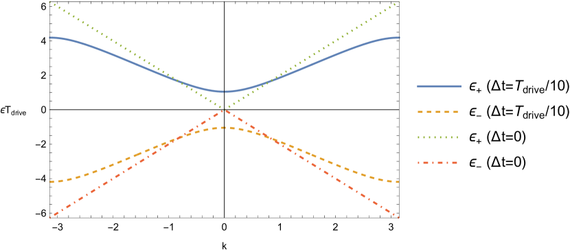
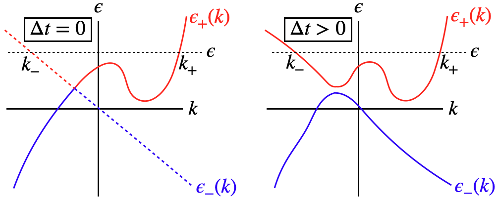
The quasienergy spectrum of is gapless at and gapped elsewhere (Fig. 1). We present the explicit calculation in Appendix A.2 for completeness. Alternatively, we can read off the solution by noting that the eigenstate problem for [Eq. (14)] is equivalent to a type of discrete-time quantum walk considered in Ref. [17]. Our parameter corresponds to the “coin” parameter of the quantum coin (see Appendix A.1 for details).
We note here that if the model is considered with open boundary conditions (by restricting the sums over to ), then the time evolution operator for a full period acts as the identity in the bulk but not at the edges. Indeed, sites at the edges ( at and a t ) gain a phase of under evolution by a full period [25]. This micromotion at the edges is similar to the anomalous edge transport that occurs in the Rudner-Lindner-Berg-Levin model in two spatial dimensions [35].
In accordance with the general arguments of Sec. II.2, we find that for a variety of disorderings of this drive, the localization length follows the behavior (15). Let us note here that the localization length can be defined in various ways depending on the boundary conditions imposed on the model; the different definitions can be expected to become equivalent in the thermodynamic limit. We present explicit definitions below.
Throughout the calculations below, we set for convenience. We write an eigenstate of [c.f. Eq. (14)] as
| (31) |
suppressing the and dependence of and , and we define
| (32) |
III.1 On-site disorder
III.1.1 Setup
We introduce two types of disorder into the SSH-type drive: phase disorder and bond disorder. In the case of phase disorder, we define a disordered loop drive by extending the clean drive at the beginning and end to include evolutions by a Hamiltonian with disordered on-site energies (exponentiating this Hamiltonian yields phase disorder). In the case of bond disorder, we follow the approach described by Eq. (21) and the discussion below there, in which we do not explicitly construct the full loop drive but instead expand about the midpoint. (We in fact consider the general combination of bond and phase disorder as an expansion about the midpoint.) Bond disorder may loosely be thought of as disorder in the hopping amplitudes of the topologically non-trivial Hamiltonian in Eq. (28b).
We introduce phase disorder using the explicit construction from Sec. II.3. In particular, we construct a disordered unitary operator and consider the drive [see Eq. (20)]. To implement phase disorder, we choose
| (33) |
where and are arbitrary phases which we later take to be disordered.
To verify that satisfies the required properties, we recall from the discussion above Eq. (20) that we must have , where is a disordered Hamiltonian that commutes with the chiral operator and is an arbitrary time interval that is sent to zero (with fixed). We may take to consist of disordered on-site energies:
| (34) |
Then it is clear then that commutes with .
We proceed to study the drive with on-site phase disorder. It is straightforward to show that the eigenstate equation (14) is equivalent to [27]
| (35a) | ||||
| (35b) | ||||
This completes the setup of the SSH-type drive with phase disorder. In this case, we have explicitly constructed a disordered, chiral-symmetric loop drive that can be studied at any in the driving period, though our main focus is on the regime of .
To introduce bond disorder, we do not explicitly construct the full loop drive for all , but instead take the approach described in Sec. II.3 of expanding about the midpoint [see Eq. (21)]. We in fact consider a slightly more general setup which includes both bond disorder and phase disorder.
We take and as given disordered operators. We consider to be as in the clean SSH-type drive with phase disorder and to be from the SSH-type drive with disorder in the hopping amplitudes; that is,
| (36a) | ||||
| (36b) | ||||
where is given by Eq. (33) and where the variables are disordered.
By a straightforward calculation, we find that the eigenstate equation (14) is equivalent to
| (37a) | ||||
| (37b) | ||||
This completes the setup of the combination of bond and phase disorder in the approach of expanding about the midpoint.
We next consider a more general problem that can be specialized to either of the two setups above. In particular, we consider the state determined by
| (38a) | ||||
| (38b) | ||||
By studying Eqs. (38a)-(38b), we can simultaneously consider both the case of phase disorder (on a disordered loop drive defined for all ) and the case of a combination of phase and bond disorder (defined explicitly only for small ). To see this, we note that setting all recovers Eqs.(35a)-(35b)], while expanding in recovers Eqs. (37a)-(37b).
Eqs. (38a)-(38b) may be brought to the following transfer matrix form:
| (39) |
where the transfer matrix is
| (40) |
Using the mapping to discrete-time quantum walks that we present in Appendix A.1, we can show that the transfer matrix (40) is a special case of a transfer matrix obtained in Ref. [17]. Note that although a -by- transfer matrix might have been expected (since we have a bipartite lattice with nearest-neighbor coupling), there is in fact a -by- transfer matrix [17]. For the case of phase disorder only, Eq. (40) was also obtained by some of the present authors in Ref. [27].
III.1.2 Localization length – calculation in position space
For our first calculation of the localization length for the problem specified by Eqs. (38a)-(38b), we use a position space approach. The time-dependent Lyapunov exponent is defined by
| (41) |
where the double brackets indicate a matrix norm (e.g., the -norm). The localization length and Lyapunov exponent are related by .
Products of random matrices have been extensively studied in the mathematics literature. In particular, a result by Schrader et al. in Ref. [33] can be applied to our present problem to yield the Lyapunov exponent to the leading order in . The final result is (see Appendix A.3.1 for details)
| (42) |
where is any site. This demonstrates that for the SSH-type drive with the on-site disorder that we have considered in this section, the localization length generically diverges with an exponent of .
III.2 Phase disorder in dimers
As a further probe of the universality of the localization length exponent, we introduce a type of phase disorder into the SSH-type drive that extends beyond individual sites. We group adjacent sites (for any integer ) into “dimers” and introduce phase disorder that couples the two sites within each dimer. We find that this drive may be described by a -by- transfer matrix. We then study this transfer matrix numerically and show that the localization length has an exponent consistent with .
We introduce dimer phase disorder into the SSH-type drive using the construction from Sec. II.3. Recall that this construction requires a disordered Hamiltonian with commutes with the chiral symmetry operator. Disorder is added to the drive by evolving with at the beginning and end for some infinitesimal time interval, resulting in a disordered drive given by Eq. (20).
A natural generalization of the on-site phase disorder considered in Sec. III.1 is to allow the disordered Hamiltonian to include both on-site terms and terms that couple sites within the same dimer (i.e., the sites and ). In order for to commute with the chiral symmetry operator, as is required for the construction of Sec. II.3, the amplitudes must not be coupled with the amplitudes. The most general such acts as some Hermitian matrix on each pair and , and as another Hermitian matrix on each pair and . The disordered unitary operator then acts as some unitary matrix on each pair and , and as another unitary matrix on each pair and .
We find it more convenient to formulate the problem in terms of the matrix elements of and , rather than in terms of the parameters of that generate these matrices. Parametrizing the disordered unitary matrices as
| (43) |
we then write disordered unitary operators for each dimer as
| (44) |
where or . The disordered unitary is then a sum over the dimers:
| (45) |
Recall from Eq. (20) and the discussion there that in the appropriate limit of the disordered evolutions at the beginning and end of the drive being taken to zero, the disordered drive may be written as . We do not yet specify the disorder distribution, but will assume that and separately are independently and identically distributed across the dimers labelled by .
We have thus defined a chirally-symmetric loop drive with phase disorder within each dimer, generalizing the on-site case considered in the previous section. We now set up the transfer matrix in order to do numerical calculations of the localization length. As the calculation is lengthy, we defer details to the Appendix and summarize the result as follows. The eigenstate equation for the drive [Eq. (14)] may be written equivalently as a transfer matrix equation involving two of the four amplitudes in adjacent dimers, and a second equation that relates the amplitudes within one dimer:
| (46a) | |||
| (46b) | |||
The transfer matrix is a function of , , , , , and (see Appendix B for the explicit expression), and the Lyapunov exponent is given by Eq. (41) with replaced by . The explicit form of the other matrix , is not needed.
We have thus brought the problem to a transfer matrix form, which is convenient for numerics. As shown in Fig. 2, we calculate the Lyapunov exponent numerically [using a definition closely related to Eq. (41)] at several values of , with results consistent with our prediction of the exponent .

It does not seem feasible, though, to obtain an analytical answer using the result from Ref. [33], because this result requires the disorder to “separate” across the transfer matrices, whereas here the disordered matrices and appear in both and .
III.3 Longer-range disorder
As a further test of the universality of the exponent , we do a numerical test using a version of disorder that extends beyond dimers. In particular, we consider disorder that decays in exponentially in real space. Due to this longer range, we cannot set up a transfer matrix calculation. We therefore impose periodic boundary conditions and use exact diagonalization to calculate the localization length numerically (see below).
We again define a disordered drive by Eqs. (19)-(20), this time using a disordered Hamiltonian that couples nearest neighbors. In particular, we take to be an independent copy of the static Anderson model (nearest-neighbor hopping with disordered on-site energies) on each sublattice:
| (47) |
Since the two sublattices are decoupled, we have the required condition that commutes with the chiral symmetry. Although only couples nearest neighbors, generally connects many sites because it is obtained by exponentiating . (In fact, it can be shown that must be exponentially local in real space [36].)
From Eq. (19), we see that the dimensionless quantities that appear in are and . We consider uniform on-site disorder; in particular, we take to be uniformly distributed (independently on each site and sublattice) in . We also set . To reduce numerical noise, we average the localization length over all quasienergies. Due to this averaging, we are testing a weaker version of (15). The numerical results are consistent with the exponent (Fig. 3).

The numerical calculation of the localization length is done as follows. At a given value of , we consider a sequence of system sizes . At each , we use exact diagonalization to find all eigenstates of . The -dependent localization length of each eigenstate is defined as the root-mean-square variation in position space:
| (48) |
where is the position operator:
| (49) |
and where the mean value is defined in the appropriate way for periodic boundary conditions [37]:
| (50) |
We are interested in the localization length in the thermodynamic limit, that is, . To calculate this, we fit the -dependent data to with fit parameters , , and . (For smaller values of , we also average over multiple disorder realizations.) This procedure is done for each eigenstate, and the average of over all eigenstates yields a data point in Fig. 3.
IV Scattering argument for the universal exponent
In the thermodynamic limit, it can be expected that the localization length should not depend on the choice of boundary conditions. We find that scattering boundary conditions (defined below) are convenient for making an analytical argument for the universality of the exponent .
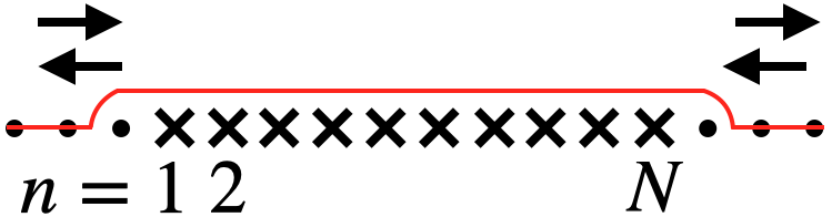
To set up the scattering problem, we write the time-dependent Hamiltonians that generate the drives and as and , respectively. We assume that the disorder in is strictly local in the following sense: we have
| (51) |
where
| (52) |
and each operator is supported on sites within a certain maximum distance of . Furthermore, this maximum distance is constant in the thermodynamic limit and independent of .
We then define a disordered “sample,” consisting of the sites , by setting for all and . The infinite regions to the right and left of the sample are the “leads.” Sufficiently far from the sample, the matrix elements of and are exactly equal. Although the matrix elements of the corresponding unitaries, and , need not be exactly equal even at long distances from the sample, they can be expected to be asympotically equal: far from the disordered region. This permits a scattering treatment for the eigenstate wavefunctions of .
Let us fix and consider the scattering problem for . Incoming and outgoing waves in the leads are described by scattering amplitudes (complex numbers), and these amplitudes are related by the S matrix of the sample (a unitary matrix denoted ). If we assume that there is only one scattering channel, then the S matrix is -by-, and there are four scattering amplitudes that may be labelled as (), where () refers to right-moving (left-moving) waves and and refer to the left and right leads. The scattering amplitudes are related by
| (53) |
Below, we argue that the single-channel case suffices to cover a wide class of drives, and we also provide a more explicit definition of the four scattering amplitudes.
The S matrix may be parametrized by transmission and reflection amplitudes:
| (54) |
In the scattering setup, localization manifests as the exponential decay of the typical transmission coefficient as increases: . From the theory of disordered systems in one dimension, the distribution of over disorder realizations becomes log-normal for large , and hence it is the average of the logarithm of the transmission coefficient that determines the typical value. In particular, we have
| (55) |
Unless (which we assume can only occur on a set of measure zero among disorder realizations), the basic relation (53) can also be written in terms of the scattering transfer matrix as
| (56) |
The unitarity of the S matrix is equivalent to the following pseudo-unitarity condition:
| (57) |
For later use, let us recall here the general parametrization of a scattering transfer matrix:
| (58) |
The basic tool in our arguments below is the following formula from Refs. [38]-[39], which (as discussed there) is a corollary to the result from Schrader et al. [33] that we referenced above. The formula applies to the case of scattering that “factorizes” into a product of individual scattering events that are disordered independently and identically. In particular: suppose that the scattering transfer matrix of the sample can be written in the product form
| (59) |
where each is a -by- scattering transfer matrix [i.e., it satisfies Eq. (57)] and where is the number of scattering events. (In the simplest case, , but we later consider the more general case of .) Suppose further that the entries of () are independently and identically distributed (i.i.d.); note that this amounts to assuming that the disorder in is uncorrelated in space and sufficiently short-ranged. Let be parametrized as in Eq. (58) (in particular with reflection amplitudes and and reflection coefficient ). Then we have 333This formula is based on assumptions that can be expected to hold for “generic” disorder distributions and model parameters. The can in fact be replaced by (i.e., the third-order terms vanish), as discussed in Refs. [38]-[39]; however, only the second-order terms are important for our present goal of showing .
| (60) |
where the subscript indicates the disorder average over any . (We emphasize that generally, the index may include more than one of the original lattice sites .)
The key point is that both terms on the right-hand side are of second order in . Thus, provided we can bring the scattering problem to the above form, it suffices to obtain , for then Eq. (60) yields the exponent in Eq. (15).
We separate the argument into two main parts. First, we consider a particular model: the SSH-type drive with on-site disorder (the same model from Sec. III, now with scattering boundary conditions). This model serves as a soluble starting point for later generalization. We obtain the required factorization into scattering transfer matrices, and we thus recover the analytical expression (42) for the inverse localization length that we obtained above using a position-space approach. In this simple problem, the number of scatterers is the same as the number of sites in the disordered sample: .
Second, we argue that the exponent can be obtained in a wider class of drives. Here we make the following modification (described in more detail below) to the scattering setup: we take the sample to consist of an alternating sequence of disordered regions and clean regions, with the disordered sites being a fixed fraction of the total number of sites in the sample. Note that setting would recover the scattering problem as stated above. In this setting, we obtain the exponent for any value by taking the scatterers in (59) to be the disordered regions within the sample (hence in this case). Eq. (60) becomes more difficult to evaluate explicitly, so we do not obtain any formula for the non-universal prefactor of the inverse localization length [i.e., the constant of proportionality in Eq. (60)]; however, we still obtain and hence . We also state the assumption that would be needed in order to obtain in the limit .
IV.1 Scattering calculation for the SSH-type drive with on-site disorder
We consider the clean drive, as defined in Sec. III, on an infinite lattice. It is straightforward to modify the phase disorder and bond disorder constructions of Sec. III.1 to the scattering setup, as we now show.
For phase disorder, we set the phases except for in the sample (). Note that the phase is offset by one unit; this is done to simplify the transfer matrices at the sample edges, and there is no effect on the large behavior. For bond disorder, we set except for . Both cases can be treated at once by using the transfer matrix defined by Eqs. (39)-(40).
We fix a time within the drive, near but not equal to , and we consider an eigenstate of with quasienergy [Eq. (14)]. The clean spectrum becomes gapless as ; for sufficiently small , the spectrum is doubly degenerate, with two momenta ( and ) corresponding to [see Fig. 1]. The eigenstates of are Bloch waves defined by [recalling Eqs. (31)-(32)]
| (61) |
where the Bloch functions are two-component “spinors” in the sublattice basis: . There are two bands; for definiteness, we take so that we are considering the upper band. (Explicit expressions are given in Appendix A.2.)
A scattering eigenstate can be written as a linear combination of Bloch waves in the leads. The coefficients are the scattering amplitudes from Eq. (53). Thus,
| (62) |
Our phase convention here (i.e., the factors of and ) is chosen for convenience.
To obtain the factorization (59), we define a matrix for converting from the basis of scattering amplitudes to the basis of position states:
| (63) |
We then have
| (64a) | ||||
| (64b) | ||||
and hence, by Eq. (39), we obtain the scattering transfer matrix (56):
| (65) |
We thus obtain the factorized form (59) with and
| (66) |
where we have identified the scatterer index with the site index (because ). It is readily checked that satisfies the pseudo-unitary condition (57).
In order to apply Eq. (60), we parametrize by , etc., as in Eq. (58). It is then straightforward to calculate and and to then use Eq. (60) to again obtain the leading order expression (42) (see Appendix A.3.2 for details).
There is a simpler way to recover Eq. (42): we note that itself satisfies the pseudo-unitarity condition (i.e., we have ). We can thus consider an auxiliary problem which is defined by taking the scattering transfer matrix for the sample to be
| (67) |
where . The localization length must be the same as the original problem because the scattering transfer matrices for the sample only differ by boundary terms: . We parametrize by , etc., as in Eq. (58). From Eq. (40), we read off and ; then applying Eq. (60) and expanding in indeed recovers Eq. (42).
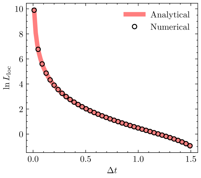
As an aside, we consider the special case of full phase disorder, i.e., each and independently and identically distributed in (and all ). We can then calculate the localization length for arbitrary via the uniform phase formula [41]: , where is the transmission coefficient of the auxiliary problem (see Appendix A.3.3 for details). The result is
| (68) |
which agrees with numerics (Fig. 4).
IV.2 Generalization to other drives
The calculation of the previous section has some features that are not representative of the generic case. First, the disordered unitary there only couples nearest neighbors, while for a generic drive, can extend further (generally it decays exponentially). Second, the clean unitary of the SSH-type drive is non-generic both in its band structure and its lack of eigenstates with complex momenta (see below).
We argue that the universal exponent is still obtained even if both of these features are relaxed. Without claiming to establish this result rigorously, we present a sequence of generalizations beyond the soluble model of the previous section, indicating the assumptions needed at each step. Mainly, we need to modify the original scattering problem by making the disordered sample have some arbitrarily small fraction of clean regions, and we need to make assumptions about the band structure of .
Beyond nearest neighbors.
Let us first consider the generalization to disorder that connects sites beyond nearest neighbors. Here, we continue to take to be the SSH-type drive as defined above. We assume for now that the disordered drive is strictly local; that is, there some range for which
| (69) |
where we suppress sublattice indices and other quantum numbers. (We later make a heuristic generalization to the case of exponential locality.) Also, we assume that the constant is independent of . The dimer disorder from Sec. III.2 provides an example of a drive with .
Due to the strict locality condition (69), the disordered unitary agrees exactly with the clean unitary throughout the leads, except for regions of size at the edges of the sample. A scattering eigenstate can therefore be written in the leads as a linear combination of Bloch waves, provided that the edge regions are avoided. In anticipation of later generalizations, let us define and . Then, a scattering eigenstate of may be written in the leads as
| (70) |
The S matrix and scattering transfer matrix of the sample are single-channel (i.e., -by-). We would like to use the analytical result (60), but we face the difficulty that, due to the higher range of in the disordered region, the scattering transfer matrix cannot be written in the factorized form (59) with i.i.d., single-channel scattering transfer matrices . (Note that a factorized form with single-channel matrices may exist, but the disorder will not be i.i.d. The dimer disorder model of Sec. III.2 illustrates this; though we worked in position space there, the scattering formulation would be similar.)
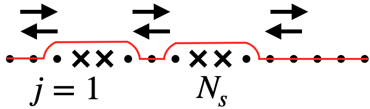
To overcome this difficulty, we modify the scattering problem in the following way. Before going into detail, let us state that the basic idea is to introduce clean regions, so that the sample is replaced by an alternating sequence of disordered and clean regions (Fig. LABEL:subfig:spacer_setup).
Each disordered region is effectively a new sample, and in particular has a -by- scattering transfer matrix. We thus obtain the factorized form (59). Our main task in the calculation below will be to show that we obtain the exponent no matter how small a fraction of the overall sample is made up of clean regions.
We proceed to describe the setup in more detail. Consider a sample of lattice sites divided into blocks of size . The total number of blocks, which we write as , is then given by
| (71) |
A parameter denotes the fraction of disordered sites within each block: the first sites of each block are disordered (we refer to this group of sites as a “disordered region”) and the remaining sites are clean. Setting corresponds to a sample with no clean regions.
We proceed to define the localization length, given any fixed fraction and any block size . At any , localization occurs and has the following effect: if we increase [with determined by Eq. (71)], the typical transmission coefficient of the auxiliary problem decays exponentially in . We may write this decay as , where the factor of is included so that is measured in units of the original lattice spacing. [As usual, we are considering the localization length at some quasienergy. The localization length also depends on , but below we will take to be determined by .]
We now show that at any fixed fraction , the exponent is obtained for . Given , we first fix a value for that is large enough to prevent any neighboring disordered regions from overlapping. In particular, we require
| (72) |
We can then write the scattering wavefunction as a linear combination of Bloch waves in all of the clean regions. We follow the same phase convention as in Eq. (70). To do this, it is convenient to write the leftmost and rightmost site in the th disordered region as
| (73a) | ||||
| (73b) | ||||
Then we may write, for any ,
| (74) |
where and . Comparing to Eq. (70), we read off and . Also, comparing to in Eq. (74), we read off
| (75) |
where we have noted that .
The scattering transfer matrix that relates to is just the scattering transfer matrix of the original problem with a different number of sites ( sites instead of ). Let us write this matrix as , bearing in mind that the subscript stands for dependence on all of the disorder variables that appear in the th disordered region. We then have
| (76) |
Collecting the last several equations, we obtain the desired factorization (59) with
| (77) |
in which the matrix multiplying on the right only introduces unimportant phase factors. By construction, the disorder dependence in the matrices is i.i.d. because the disordered regions have no overlap. Thus, Eq. (60) applies. In particular, in units of the original lattice spacing we have
| (78) |
To complete the calculation, we show next that the reflection amplitude of an individual block satisfies . The essential point is to show , where is the reflection amplitude associated with ; once this is shown, we can easily account for the time dependence introduced by the phase factors that appear in Eq. (77). Indeed, from Eq. (77) and the general parametrization (58), we read off
| (79a) | ||||
| (79b) | ||||
From (72), we see that it suffices to take to be, e.g., ; in particular, is then just a number (independent of ). The momenta depend on in a regular way, i.e., . Thus, we conclude that it is enough to show .
To show , we start by considering two different limits of the original problem scattering problem: (1) If we fix and send the sample size to infinity, then the magnitude of the sample reflection amplitude goes to unity due to localization (). This is the regime we are interested in. However, for the purpose of treating each disordered region as a version of the original problem, it is useful to consider a different limit, as we now explain. (2) If we fix the system size and expand in , then generically we obtain . We can see this by noting that the reflection amplitude must vanish at (since the midpoint has perfect transmission), and that the first correction will generically be linear in due to expanding the propagator.
In the present case, we just need to apply (2) to each disordered region. The size of each disordered region () is determined entirely by and ; in particular, it is independent of . Thus, we generically have . From Eqs . (60), we thus obtain , i.e., holds for any .
Throughout the above argument, we have assumed to be strictly local [Eq. (69)]. However, a generic drive is only exponentially local, i.e., for sufficiently large we have
| (80) |
for some constants and that are independent of . We assume that we can replace and for some -independent constants and . Then, we repeat the above arguments with fixed to any particular value satisfying . Although the disordered unitary then differs slightly from the clean unitary even in the clean regions, the difference can be made arbitrarily small.
Finally, let us conclude by considering the limit , which corresponds to a scattering problem with a single disordered region. Our argument above yields the small expansion for some unknown function . Noting from (72) that as , we see that can be obtained in the limit given the assumption that .
Generalization of the clean drive.
We next generalize beyond the particular case of the SSH-type drive. Here we note that the precise forms of the Bloch function and of the two momenta were not important in our calculation above; the essential point was that the S matrix for the sample was single-channel. We can therefore generalize our calculation to include any quasienergy at which has two-fold degeneracy for all in some neighborhood of .
Let us consider the case that has two bands, which we write as . In momentum space, the block-diagonal form (11) becomes
| (81) |
where, by assumption, and have winding numbers and , respectively. The corresponding quasienergy spectra and must go from to , but need not do so monotonically. Example spectra are sketched in Fig. 6.
For close to but not equal to , gaps open at all band crossings. We define and to be the upper and lower bands, respectively, and we focus for now on the midpoint of the drive, at which the bands are defined by taking the limit as . [Note that the bands at the midpoint are not the same as and .] As is clear from Fig. 6, there is generically some range of quasienergies that have a two-fold degeneracy with the two associated momenta moving in opposite directions. It is for in this range that our argument straightforwardly applies.
Let us explain this more detail. For in some range, we have , , and , where is the group velocity. [Here we assume for definiteness that lies in the upper band.] Although we have considered at the midpoint (), allowing to vary slightly from the midpoint does not change the qualitative features; there remains a similar range of quasienergies with the desired two-fold degeneracy. For quasienegies in this range, and for sufficiently close to the midpoint, the eigenstates of are linear combinations of two (time-dependent) Bloch waves. We have thus brought our localization problem, for a more general class of topologically non-trivial drives, into the framework of single-channel scattering, at least for some range of quasienergies.
We now present the scattering argument for the exponent in this more general setting. A complication arises, both in the basic setup of the scattering problem and in our argument about inserting clean regions: although by assumption has two bands, it may have eigenstates with complex momenta when confined either to a half-line or to a finite region. These eigenstates grow or decay exponentially in position space; schematically, for some decay length . [We emphasize that this length scale is distinct from the operator decay length that appears in Eq. (80). Even a strictly local can have exponentially decaying eigenstates, although the SSH-type drive of Sec. III does not.] When we introduce disorder into the sites , the edge sites ( and ) can then be regarded as endpoints of half-lines that extend into the leads. This implies that the eigenstate wavefunction in the leads is generally not a linear combination solely of Bloch waves [even at distances greater than away from the sample]; there can also be contributions from modes that decay as . The solution is simple: as usual in scattering theory, the expansion in terms of Bloch waves [Eq. (70)] holds for .
Similarly, we must note that the exponentially growing and decaying eigenstates of can appear in each inserted clean region [even at distances greater than from the nearest disordered region]. To deal with this, we assume that the decay lengths of the eigenstates of can be uniformly bounded, in the sense that there is a fixed distance , independent of , for which for all (in some neighborhood of ). We choose the constant to be much greater than , i.e., satisfies
| (82) |
Then, the expansions in terms of Bloch waves – both the basic setup [Eq. (70)] and the more general expansions within each clean region [Eq. (74)] hold as written (up to error that can be decreased arbitrarily by increasing ). From this point onward, our argument for the exponent proceeds exactly as in the case that was taken to be the SSH-type drive.
Thus, we have obtained the exponent provided that we consider a quasienergy at which the clean drive (evaluated at the midpoint) has two-fold degeneracy. In the generic two-band case, there is a range of for which this condition holds.
V Conclusion
We considered the class AIII of Floquet drives in one spatial dimension, and we argued that drives in this class that the topological invariant equal to one exhibit a localization-delocalization transition with a universal exponent. We argued that the localization length diverges at a particular time (the midpoint of the loop part of the drive), throughout the quasienergy spectrum. We obtained the exponent explicitly in a simple model, checked it numerically in more complicated models, and provided an analytical argument for a still larger class of models (based on some plausible assumptions). Based on numerical evidence, we believe that some assumptions of the analytical argument are not essential.
A natural follow-up to this work would be to consider the effect of interactions. The SSH-type drive we have considered readily extends to an interacting spin model; note also that the interacting generalization of the flow index is known from Ref. [30]. The interacting generalization of our work may provide an interesting example of a localization-delocalization transition in a Floquet-many-body-localized setting.
Acknowledgements.
We thank Victor Gurarie, Curt von Keyserlingk, and Shivaji Sondhi for useful discussions on related topics. This work used computational and storage services associated with the Hoffman2 Shared Cluster provided by UCLA Institute for Digital Research and Education’s Research Technology Group. A.B.C., P.S., and R.R. acknowledge financial support from the University of California Laboratory Fees Research Program funded by the UC Office of the President (UCOP), grant number LFR-20-653926. A.B.C acknowledges financial support from the Joseph P. Rudnick Prize Postdoctoral Fellowship (UCLA). P.S. acknowledges financial support from the Center for Quantum Science and Engineering Fellowship (UCLA) and the Bhaumik Graduate Fellowship (UCLA).Appendix A Further details for the SSH-type drive with on-site disorder
A.1 Mapping to discrete-time quantum walk
In the main text, we showed that the eigenstate problem [Eq. (14)] becomes Eqs. (38a)-(38b) in position space. Here, we show that these equations are equivalent to a special case of the generalized discrete-time quantum walk studied in Ref. [17]. We start by reviewing the setup for the discrete-time quantum walk [17].
The discrete-time quantum walk occurs on an infinite chain with a two-component “spin” degree of freedom (, ) at each site; a general state is written as . A single time step is implemented by a unitary operator , where the “shift” moves up (down) spins one unit to the right (left) and where acts on the spin degree of freedom at each site as a unitary -by- matrix . The matrix is parameterized by , and (in the same way as in Eq. (1) of Ref. [17]).
The eigenstate equation for the discrete-time quantum walk problem is . In position space, the eigentate equations become Eqs. (H1a)-(H2b) of Ref. [39]. Our Eqs. (38a)-(38b) are in fact special cases of (H1a)-(H2b) [with relabelled as in (H1a) and as in (H2b)] with the following choice of parameters:
| (83a) | ||||
| (83b) | ||||
| (83c) | ||||
| (83d) | ||||
and with the following correspondence of the basic variables:
| (84) |
Using this mapping, we can reproduce some of the results below by translating results from the discrete-time quantum walk case. However, for completeness we present the calculations directly in the case of the SSH-type drive.
A.2 Solution of the clean model
By Bloch’s theorem, a wavefunction that solves the eigenstate equation (14) with some quasienergy can be written as
| (85) |
where the Bloch function is a two-component “spinor” in the sublattice index:
| (86) |
We proceed to solve for the quasienergies and Bloch functions. From now on we assume that are in the middle section of the drive (). We remove the disorder from Eqs. (35a)-(35b) (by setting all ) to obtain
| (87a) | ||||
| (87b) | ||||
Substituting in the plane wave form given above, we obtain
| (88) |
which we then solve to find the two bands of the model (denoted and ). The quasienergies of the two bands are are defined (modulo ) by
| (89) |
and the unit-normalized Bloch spinors are
| (90) |
where the prefactor of is chosen for convenience and where is a normalization factor:
| (91) |
The first Brilluoin zone is and is fixed by requiring . The resulting two bands are shown in Fig 1.
A.3 Calculation of the localization length
A.3.1 Position space calculation
Here we obtain Eq. (42) using a result from Schrader et al. [33]. For a summary of their setup in a notation similar to that used in this paper, and also for a calculation that includes that below as a special case (using the mapping from Appendix A.1), see Appendix B of Ref. [39].
As we point out in the main text, the (position-space) transfer matrix satisfies . Ref. [33] instead considers matrices satisfying the same condition with replaced by ; however, as they point out, the two types of matrix are isomorphic. We therefore start by defining a matrix that is isomorphic to : in particular, , where the unitary matrix is given by [33]
| (92) |
Then satisfies the condition.
Eq. (41) can be written in terms of the matrices as
| (93) |
Note that in passing from Eq. (41) to Eq. (93), we dropped boundary terms that make no contribution in the limit .
Ref. [33] calculates (93) to leading order in a small parameter which is given in our case by . In order to use the result from Ref. [33], we must verify that (there denoted ) satisfies the necessary properties. First, we check that the matrices commute with each other at . At the point , we have
| (94) |
which implies in particular that ; then the same is true for the matrices, by linearity. Second, we must check the trace condition , which in our case reduces to
| (95) |
At worst, the left-hand side can equal , but only in a “fine-tuned” case; generically, the inequality is satisfied.
We then define
| (96a) | ||||
| (96b) | ||||
| (96c) | ||||
Note that is real and traceless. We then have, by a straightforward calculation, a parametrization of the form of Eq. (8) from Ref. [33]:
| (97) |
where is the -by- matrix that rotates by the angle . [Eq. (8) in Ref. [33] also includes a matrix , which is in our case the identity matrix, and another matrix that is not needed for our purposes.] The constant defined (in a slightly different notation) by Eq. (9) from Ref. [33] is then found to be
| (98) |
Finally, substituting Eqs. (96a) and (98) into Eq. (22) of Ref. [33] yields Eq. (42) from the main text.
A.3.2 Scattering calculation
In Sec. IV.1, we obtained the inverse localization length at leading order in [Eq. (42)] by applying the scattering formula (60) to the auxiliary problem defined by Eq. (67). This required us to show that the auxiliary problem has the same localization length as the original problem. In this section, we apply Eq. (60) directly to the original problem, yielding the same result (42).
Without loss of generality, we fix and consider . The scattering momentum and the Bloch function vary with . Expanding in , we readily obtain
| (99a) | ||||
| (99b) | ||||
| (99c) | ||||
Then, from Eqs. (40), (63), and (66), we calculate the scattering transfer matrix as an expansion in . We only need the reflection amplitudes at linear order in , and they can be obtained straightforwardly using the general parametrization (58):
| (100a) | ||||
| (100b) | ||||
Substitution into Eq. (60) yields Eq. (42) from the main text once again.
A.3.3 Full phase disorder
In order to obtain Eq. (68), we start by recalling a result from Ref. [41]. Consider a general scattering problem in which we have the factorization (59) with (hence we will write ). Let be parametrized by , , , and , as in Eq. (58). If, at sufficiently large system size , we have the following phase uniformity condition:
| (101) |
then Ref. [41] shows
| (102) |
where is the transmission coefficient and where the disorder average is taken over any site . Since , one simple case in which the condition (101) holds is the following: is distributed uniformly in , independently of .
We now apply this result to the SSH-type drive with on-site phase disorder. (We do not consider bond disorder because this was only defined for times near the midpoint, whereas here our concern is to find an answer for all .) It is simplest to work with the auxiliary problem defined by Eq. (67). Setting in Eq. (40), we read off and . Thus, if is uniformly distributed in , then the condition (101) holds, and (102) yields Eq. (68) from the main text.
Appendix B Transfer matrix for the SSH-type drive with dimer disorder
Here we derive the transfer matrix relation (46a) and the explicit expression for the transfer matrix for the sites. To simplify the notation, we re-label the four sites , , and as ,, and , respectively. We write the disordered unitary matrices ( or ) as
| (103) |
It is straightforward to show that the eigenstate equation (14) becomes the following four equations in position space:
| (104a) | ||||
| (104b) | ||||
| (104c) | ||||
| (104d) | ||||
We use the second and third equations to eliminate and [this is expressed by Eq. (46b)]. From the first and fourth equations, we then obtain
| (105) |
where the transfer matrix is given below. Note that this is the same as Eq. (46a) from the main text.
To present the transfer matrix, we first define
| (106a) | ||||
| (106b) | ||||
| (106c) | ||||
| (106d) | ||||
Then the transfer matrix is
| (107) |
with the following matrix elements:
| (108a) | ||||
| (108b) | ||||
| (108c) | ||||
| (108d) | ||||
References
- Huckestein [1995] B. Huckestein, Reviews of Modern Physics 67, 357 (1995).
- Ippoliti and Bhatt [2020] M. Ippoliti and R. N. Bhatt, Physical Review Letters 124, 086602 (2020).
- Kitaev [2009] A. Kitaev, AIP Conference Proceedings 1134, 22 (2009).
- Kagalovsky and Nemirovsky [2008] V. Kagalovsky and D. Nemirovsky, Physical Review Letters 101, 127001 (2008).
- Evers and Mirlin [2008] F. Evers and A. D. Mirlin, Reviews of Modern Physics 80, 1355 (2008).
- Song and Prodan [2014] J. Song and E. Prodan, Physical Review B 89, 224203 (2014).
- Song et al. [2014] J. Song, C. Fine, and E. Prodan, Physical Review B 90, 184201 (2014).
- Mondragon-Shem et al. [2014] I. Mondragon-Shem, T. L. Hughes, J. Song, and E. Prodan, Physical Review Letters 113, 046802 (2014).
- Altland et al. [2015] A. Altland, D. Bagrets, and A. Kamenev, Physical Review B 91, 085429 (2015).
- Morimoto et al. [2015] T. Morimoto, A. Furusaki, and C. Mudry, Physical Review B 91, 235111 (2015).
- Titum et al. [2015] P. Titum, N. H. Lindner, M. C. Rechtsman, and G. Refael, Physical Review Letters 114, 056801 (2015).
- Roy and Sreejith [2016] S. Roy and G. J. Sreejith, Physical Review B 94, 214203 (2016).
- Titum et al. [2017] P. Titum, N. H. Lindner, and G. Refael, Physical Review B 96, 054207 (2017).
- Obuse and Kawakami [2011] H. Obuse and N. Kawakami, Physical Review B 84, 195139 (2011).
- Kitagawa [2012] T. Kitagawa, Quantum Information Processing 11, 1107 (2012).
- Rakovszky and Asboth [2015] T. Rakovszky and J. K. Asboth, Physical Review A 92, 052311 (2015).
- Vakulchyk et al. [2017] I. Vakulchyk, M. V. Fistul, P. Qin, and S. Flach, Physical Review B 96, 144204 (2017).
- Derevyanko [2018] S. Derevyanko, Scientific Reports 8, 1795 (2018).
- Kitagawa et al. [2010] T. Kitagawa, M. S. Rudner, E. Berg, and E. Demler, Physical Review A 82, 033429 (2010).
- Shtanko and Movassagh [2018] O. Shtanko and R. Movassagh, Physical Review Letters 121, 126803 (2018).
- Wauters et al. [2019] M. M. Wauters, A. Russomanno, R. Citro, G. E. Santoro, and L. Privitera, Physical Review Letters 123, 266601 (2019).
- Gannot [2015] Y. Gannot, Effects of Disorder on a 1-D Floquet Symmetry Protected Topological Phase (2015), arXiv:1512.04190.
- Harper et al. [2020] F. Harper, R. Roy, M. S. Rudner, and S. Sondhi, Annual Review of Condensed Matter Physics 11, 345 (2020).
- Roy and Harper [2017] R. Roy and F. Harper, Physical Review B 96, 155118 (2017).
- Liu et al. [2018] X. Liu, F. Harper, and R. Roy, Physical Review B 98, 165116 (2018).
- Note [1] In particular, is the localization length for the time-periodic Floquet states of the operator considered as if were the full period.
- Brown [2019] A. Brown, Geometric Current Response in Chern Systems and Topological Delocalization in Floquet Class AIII Systems, Ph.D. thesis, UCLA (2019).
- Sathe [2023] P. S. Sathe, Aspects of Localization in Topological Insulators, Ph.D. thesis, UCLA (2023).
- Kitaev [2006] A. Kitaev, Annals of Physics 321, 2 (2006).
- Gross et al. [2012] D. Gross, V. Nesme, H. Vogts, and R. F. Werner, Communications in Mathematical Physics 310, 419 (2012).
- Note [2] Forthcoming work.
- Liu et al. [2022] T. Liu, X. Xia, S. Longhi, and L. Sanchez-Palencia, SciPost Physics 12, 027 (2022).
- Schrader et al. [2004] R. Schrader, H. Schulz-Baldes, and A. Sedrakyan, Annales Henri Poincaré 5, 1159 (2004).
- Su et al. [1979] W. P. Su, J. R. Schrieffer, and A. J. Heeger, Physical Review Letters 42, 1698 (1979).
- Rudner et al. [2013] M. S. Rudner, N. H. Lindner, E. Berg, and M. Levin, Physical Review X 3, 031005 (2013).
- Graf and Tauber [2018] G. M. Graf and C. Tauber, Annales Henri Poincaré 19, 709 (2018).
- Resta [1998] R. Resta, Physical Review Letters 80, 1800 (1998).
- Culver et al. [2022a] A. B. Culver, P. Sathe, and R. Roy, Scattering Expansion for Localization in One Dimension (2022a), arXiv:2210.07999.
- Culver et al. [2022b] A. B. Culver, P. Sathe, and R. Roy, Scattering Expansion for Localization in One Dimension: from Disordered Wires to Quantum Walks (2022b), arXiv:2211.13368.
- Note [3] This formula is based on assumptions that can be expected to hold for “generic” disorder distributions and model parameters. The can in fact be replaced by (i.e., the third-order terms vanish), as discussed in Refs. [38]-[39]; however, only the second-order terms are important for our present goal of showing .
- Anderson et al. [1980] P. W. Anderson, D. J. Thouless, E. Abrahams, and D. S. Fisher, Physical Review B 22, 3519 (1980).