Evaluating the reconstruction of individual haloes in constrained cosmological simulations

Abstract

Constrained cosmological simulations play an important role in modelling the local Universe, enabling investigation of the dark matter content of local structures and their formation histories. We introduce a method for determining the extent to which individual haloes are reliably reconstructed between constrained simulations, and apply it to the Constrained Simulations in BORG (CSiBORG) suite of $101$ high-resolution realisations across the posterior probability distribution of initial conditions from the Bayesian Origin Reconstruction from Galaxies (BORG) algorithm. The method is based on the overlap of the initial Lagrangian patch of a halo in one simulation with those in another, and therefore measures the degree to which the haloes’ particles are initially coincident. By this metric we find consistent reconstructions of $M\gtrsim 10^{14}~{}M_{\odot}/h$ haloes across the CSiBORG simulations, indicating that the constraints from the BORG algorithm are sufficient to pin down the masses, positions and peculiar velocities of clusters to high precision. The effect of the constraints tapers off towards lower mass however, and the halo spins and concentrations are largely unconstrained at all masses. We document the advantages of evaluating halo consistency in the initial conditions, describe how the method may be used to quantify our knowledge of the halo field given galaxy survey data analysed through the lens of probabilistic inference machines such as BORG, and describe applications to matched but unconstrained simulations.

1 Introduction

The dynamics of the Universe are largely governed by DM, constituting the majority of the matter content of the Universe. Over the past decades, cosmological simulations have emerged as the paramount instrument to elucidate its nonlinear dynamics and interplay with baryons (Wechsler & Tinker, 2018; Vogelsberger et al., 2020; Angulo & Hahn, 2022). Simulations typically employ IC based on a fixed power spectrum and random phases of the primordial matter field (Press & Schechter, 1974; Davis et al., 1985; Lacey & Cole, 1993; Eisenstein & Hut, 1998; Tinker et al., 2008). However, such IC produce universes that resembles the real Universe only statistically, but cannot be linked object-by-object.

The alternative is the “constrained simulation”, in which not only the amplitudes but also the phases of the primordial density perturbations are encoded. The beginnings of this endeavour can be traced back to Hoffman & Ribak (1991), who laid down the foundation for simulating constrained realisations of Gaussian random fields. Local Universe constraints were subsequently derived from galaxy counts (Kolatt et al., 1996; Bistolas & Hoffman, 1998), peculiar velocity measurements (van de Weygaert & Hoffman, 2000; Klypin et al., 2003; Kravtsov et al., 2002) and galaxy groups (Wang et al., 2014), which, together with advances in simulation resolution, gravity modelling, IC generation or galaxy bias modelling, have led to local Universe simulation becoming a mature field.

Deriving the IC that generated the structure we see around us is an inference problem, and, as we have only one Universe, is best formulated in a Bayesian framework. This realisation led to the development of a Bayesian forward-modelling approach now known as the BORG algorithm (Jasche & Wandelt, 2013; Jasche et al., 2015; Lavaux & Jasche, 2016; Jasche & Lavaux, 2019). BORG leverages an efficient Hamiltonian Markov Chain Monte Carlo algorithm to sample the initial matter field along with parameters associated with observational selection effects, galaxy bias and cosmology. The BORG posterior encapsulates all realisations of the local Universe that are compatible with the observational constraints used to derive them. The flagship application of BORG—and the one that we will use in this work—targeted the $\mathrm{2M}\texttt{++}$ galaxy catalogue, a whole sky redshift compilation of $69,160$ galaxies (Lavaux & Jasche, 2016; Jasche & Lavaux, 2019) based on the Two-Micron-All-Sky Extended Source Catalog (Skrutskie et al., 2006). Work is in progress to augment the constraints with information from cosmic shear (Porqueres et al., 2021) and peculiar velocities (Prideaux-Ghee et al., 2023).

In this work, we use the CSIBORG suite of constrained cosmological simulations (Bartlett et al., 2021; Desmond et al., 2022), which are based on the BORG $\mathrm{2M}\texttt{++}$ IC. Each CSIBORG box is a resimulation of IC from a single BORG posterior sample inferred from the $\mathrm{2M}\texttt{++}$ galaxy catalogue (Lavaux & Jasche, 2016; Jasche & Lavaux, 2019), so that differences between realisations quantify the reconstruction uncertainty associated with our incomplete knowledge of the galaxy field and galaxy–halo connection. Hutt et al. (2022) used CSIBORG to study the effect of the reduced cosmic variance on the HMF and clustering of haloes, and developed a method to assess the consistency of halo reconstruction from the final conditions. CSIBORG has also previously been used to create catalogues of local voids-as-antihalos (Desmond et al., 2022), and search for modified gravity (Bartlett et al., 2021) and dark matter annihilation and decay (Bartlett et al., 2022; Kostić et al., 2023). Beyond the CSIBORG suite, a focus of constrained simulations has been used to study the Local Group and its assembly history, e.g. within the CLUES (Gottloeber et al., 2010; Sorce et al., 2016) and SIBELIUS (Sawala et al., 2022; McAlpine et al., 2022) projects. They have also been used to study the connection between Sloan Digital Sky Survey galaxies and their haloes (Wang et al., 2016; Yang et al., 2018; Zhang et al., 2022; Xu et al., 2023), quantify the compatibility of the local Universe with $\Lambda\mathrm{CDM}$ (Stopyra et al., 2021, 2023) and model the local Universe in modified gravity (Naidoo et al., 2023).

Due to their Bayesian setup, BORG and CSIBORG afford quantification of the effects of data and model uncertainties on the dark matter distribution produced in the simulations. An alternative method leverages the Wiener filter, which allows reconstruction of the mean field but cannot quantify the reconstruction uncertainty (Hoffman & Ribak, 1991; Zaroubi et al., 1995, 1999; Doumler et al., 2013a, b; Hoffman et al., 2015). In a recent study, Valade et al. (2023) compared a Wiener filter- and Bayesian-based (HAMLET; Valade et al. 2022) approach to reconstruction from a mock peculiar velocity catalogue. They found that the two to agree for nearby structures ($\lesssim 40~{}\mathrm{Mpc}/h$) but that at greater distances the Bayesian method outperforms the Wiener filter reconstruction.

The objective of our study is to investigate the robustness of the reconstructions of individual haloes in constrained cosmological simulations. We develop a framework to assess whether a halo present in one box is also present in another, and hence what properties of the halos are reliably reconstructed across the suite. This is achieved by means of a novel metric, the overlap of haloes’ initial Lagrangian patches. While the method is agnostic as to the way in which the simulations of the suite are linked, a natural application (and the one on which we focus) is to suites that sample the IC posterior of a prior inference. We showcase the method by application to CSIBORG, where we quantify the consistency of halo reconstruction as a function of various halo properties. The significance of the results are established by contrast with Quijote, an unconstrained suite.

Other applications of our method include matching haloes between DM-only simulations and their hydrodynamical counterparts, as well as simulations using different cosmological models, e.g. $\Lambda\mathrm{CDM}$ and modified gravity. While traditional methods for matching haloes between different runs often depend on a consistent DM particle ordering between the runs (e.g. Butsky et al. 2016; Desmond et al. 2017; Mitchell et al. 2018; Cataldi et al. 2021), ours does not. In both above-mentioned scenarios, our approach can quantify how either the hydrodynamics or the cosmology impacts the properties of individual haloes, instead of relying solely on population statistics conditioned on properties such as mass (e.g. Pallero et al. 2023).

The structure of the paper is as follows. In Section 2 we introduce the two sets of simulations employed in our work, in Section 3 we introduce the overlap metric and its interpretation,  Section 4 contains our results and in Section 5 we discuss the results. Lastly, we conclude in Section 6. All logarithms in this work are base-10.

2 Simulated data

In this section we describe the two sets of simulations that we use, CSIBORG and Quijote, and their halo catalogues.

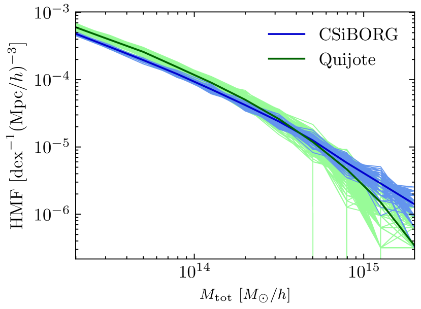
Figure 1: The FOF HMF in CSIBORG and Quijote. The thin background lines show the realisations of CSIBORG and Quijote and the bold lines show their mean. The CSIBORG HMF undershoots and overshoots the Quijote HMF at low and high masses, respectively. The lower limit is approximately given by Quijote haloes containing $100$ particles.

2.1 CSiBORG

The CSIBORG suite, first presented in Bartlett et al. (2021), consists of $101$ DM-only $N$-body simulations in a $677.7~{}\mathrm{Mpc}/h$ box centred on the MW, with IC sampled from the BORG reconstruction of the $\mathrm{2M}\texttt{++}$ galaxy survey (Lavaux & Jasche, 2016). This reconstruction covers the same volume as each CSIBORG box, discretised into $256^{3}$ cells for a spatial resolution of $2.65~{}\mathrm{Mpc}/h$ (Jasche & Lavaux, 2019). The BORG density field is constrained within a spherical volume of radius $\sim 155~{}\mathrm{Mpc}/h$ around the MW, where the $\mathrm{2M}\texttt{++}$ catalogue has high completeness.

In CSIBORG, the IC are propagated linearly to $z=69$ and augmented with white noise on a $2048^{3}$ grid in the central high-completeness region, corresponding to a spatial resolution of $0.33~{}\mathrm{Mpc}/h$ and a DM particle mass of $3.09\times 10^{9}~{}\mathrm{M}_{\odot}/h$. To ensure a smooth transition to the remainder of the box, a buffer region of approximately $10~{}\mathrm{Mpc}/h$ is added at the edge of the high-resolution region. Both BORG and CSIBORG adopt the cosmological parameters from the Planck Collaboration et al. (2014) best fit results, including the WMAP polarisation, high multipole moment, and baryonic acoustic oscillation data, except $H_{0}$ which is taken from the 5-year WMAP results combined with Type Ia supernovae and baryonic acoustic oscillation data (Hinshaw et al., 2009) ($T_{\mathrm{CMB}}=2.728~{}\mathrm{K}$, $\Omega_{\mathrm{m}}=0.307$, $\Omega_{\Lambda}=0.693$, $\Omega_{\mathrm{b}}=0.04825$, $H_{0}=70.5~{}\mathrm{km}~{}\mathrm{s}^{-1}~{}\mathrm{Mpc}^{-1}$, $\sigma_{8}=0.8288$, $n=0.9611$). The DM density field is evolved to $z=0$ using the adaptive mesh refinement code RAMSES (Teyssier, 2002), where only the central high-resolution region is refined (reaching level $18$ by $z=0$ with a spatial resolution of $2.6~{}\mathrm{kpc}/h$).

As we will be studying the reconstruction of individual objects, whose initial Lagrangian patches are constrained in BORG, it is illustrative to consider how many BORG cells constitute the Lagrangian patch of a halo. We find this to be approximately $N\approx 7~{}M_{\rm tot}/(10^{13}M_{\odot}/h)$. BORG constrains the average field value in each cell with physical size $2.65~{}\mathrm{Mpc}/h$, and we do not a-priori expect haloes with Lagrangian patches spanning only a few BORG cells to be consistently reconstructed in CSIBORG since such haloes likely vary strongly across the BORG posterior. However, haloes above $\sim 10^{14}~{}\mathrm{Mpc}/h$ comprise initially $\gtrsim 100$ cells and are therefore likely well constrained.

2.2 Quijote

We compare the CSIBORG results to the publicly available Quijote simulations (Villaescusa-Navarro et al., 2020). Quijote is a suite of unconstrained simulations evolved from $z=127$ to $z=0$ using the GADGET-III code (Springel et al., 2008). We use $10$ realisations of the Quijote DM-only simulations with randomly drawn IC phases, each with a volume of $1~{}\mathrm{Gpc}/h$ and a particle mass of $8.72\times 10^{10}~{}\mathrm{M}_{\odot}/h$ in a fiducial cosmology: $\Omega_{\mathrm{m}}=0.3175$, $\Omega_{\Lambda}=0.6825$, $\Omega_{\mathrm{b}}=0.049$, $H_{0}=67.11~{}\mathrm{km}~{}\mathrm{s}^{-1}~{}\mathrm{Mpc}^{-1}$, $\sigma_{8}=0.834$ and $n=0.9624$. Besides the constraints, the most significant difference with CSIBORG is the volume, so for an approximately fair comparison when calculating any extrinsic quantity we mimic the CSIBORG high-resolution region by splitting each Quijote box into $27$ non-overlapping spherical sub-volumes of radius $155~{}\mathrm{Mpc}/h$ centreed at $n\times 155~{}\mathrm{Mpc}/h$ for $n=1,3,5$ along each axis.

2.3 Halo catalogues

We use the FOF halo finder (FOF; Davis et al. 1985) in both CSIBORG and Quijote, with a linking length parameter of $b=0.2$. FOF connects particles within a distance $b$ times the mean inter-particle separation. FOF can create artificially large structures by connecting extraneous particles to haloes along nearby filaments of the density field, particularly for merging haloes at $z=0$ (Eisenstein & Hut, 1998). Warren et al. (2006) and Lukić et al. (2009) proposed corrections to this based on particle number and halo concentration respectively, but as we do not require high-precision halo masses we do not apply them here.

To reduce numerical resolution errors of recovered haloes and their properties, authors have suggested that haloes must contain at least $50-100$ particles (Springel et al., 2008; Onions et al., 2012; Knebe et al., 2013; van den Bosch & Jiang, 2016; Griffen et al., 2016), though Diemer & Kravtsov (2015) suggested stricter criteria for measuring e.g. concentration to avoid having only a few particles in the inner parts of the halo, especially if the inner region spans only a few force resolution lengths. Recently, van den Bosch & Ogiya (2018) proposed a more stringent criterion for determining the numerical convergence of infalling subhaloes. However, in this work we are not concerned with substructure or halo profiles, and thus adopt the simpler and less restrictive criterion of $100$ particles for all haloes, corresponding to a minimum halo mass of $3.09\times 10^{11}~{}\mathrm{M}_{\odot}/h$ and $8.72\times 10^{12}~{}\mathrm{M}_{\odot}/h$ for CSIBORG and Quijote, respectively. In CSIBORG we identify haloes only inside the high-resolution region. As CSIBORG has a mass-resolution nearly two orders of magnitude better than Quijote, when comparing the two simulations we only consider haloes above the mass-resolution of Quijote.

CSIBORG and Quijote assume different cosmological parameters, yielding a difference in both the large-scale structure and halo population. Hutt et al. (2022) study how this affects the HMF, finding insignificant disparities due to the different cosmologies. They do however quantify the reduced spread of the HMF of individual CSIBORG realisations relative to Quijote due to the suppression of cosmic variance by the IC constraints. We show the HMF in Fig. 1. It is found that the CSIBORG and Quijote HMFs have some systematic disagreement, with the former predicting higher bright-end abundances (see also McAlpine et al. 2022; Desmond et al. 2022; Hutt et al. 2022). However, this becomes statistically significant only above $M\sim 10^{15}M_{\odot}/h$. On the other hand, CSIBORG systematically undershoots the Quijote HMF below $\sim 10^{14.2}~{}M_{\odot}/h$. These discrepancies have recently been investigated by Stopyra et al. (2023) who showed that replacing the $10$-step particle mesh solver used in the BORG forward model with a $20$-step COLA solver (Tassev et al., 2013) corrects for them.

3 Methodology

We aim to develop a metric to quantify the extent to which halos are reliably reconstructed between boxes, e.g. across the simulations of constrained suites. We do so by evaluating the similarity of proto-haloes at high redshift, measured by their initial Lagrangian patches. This is a priori a sensible approach as it is the initial conditions that are constrained: focusing on the initial snapshot facilitates the establishment of a more causally coherent framework, circumventing reliance on interpretations deduced purely from the final conditions as in e.g. Hutt et al. (2022). Most of our work is intended to interpret and show it to be useful a posteriori as well.

Similar approaches are used to associate haloes between DM-only and hydrodynamical simulations sharing the same IC (e.g. Butsky et al. 2016; Desmond et al. 2017; Mitchell et al. 2018; Cataldi et al. 2021). For instance, Desmond et al. leverage the ability to match DM particle IDs between DM-only and hydrodynamical runs to match haloes as follows: if halo $a$ from the DM-only run shares the most particles with halo $b$ from the hydrodynamical run, and conversely $b$ shares most particles with $a$, they are identified as a match. This bears strong resemblance to the method we develop because the particle IDs are assigned based on their position in the initial snapshot. In CSIBORG the particle IDs are not consistent between realisations so this method cannot be used directly.

We cross-correlate two IC realisations as follows. We denote the first simulation as the “reference” and the second as the “crossing” simulation and calculate the overlap of each halo in the reference simulation with all haloes in the crossing simulation. We identify FOF haloes in the final snapshot of both the reference $\mathcal{A}$^th and crossing $\mathcal{B}$^th IC realisation and trace their constituent particles back to the initial snapshot. To calculate the intersecting mass of a halo $a\in\mathcal{A}$ and $b\in\mathcal{B}$, we use the NGP scheme to assign the halo particles to a $2048^{3}$ grid in the initial snapshot, matching the initial refinement of the high-resolution region. We denote the mass assigned to a single cell $m_{a}$ and $m_{b}$, respectively, for the two haloes. On the same grid we also calculate the background mass field of all particles assigned to a halo in the final snapshot in the respective simulation, $\widehat{m}_{\mathcal{A}}$ and $\widehat{m}_{\mathcal{B}}$.

In the NGP scheme, a particle located at $x_{i}\in\left[0,1\right]$ along the $i$^th axis is assigned to the $\lfloor x_{i}N_{\rm cells}\rfloor$^th cell, where $N_{\rm cells}$ is the total number of cells along an axis. We then apply a Gaussian smoothing to the NGP field using a kernel width of one cell and define the intersecting mass of haloes $a$ and $b$ as

$$X_{ab}\equiv\sum_{n}\frac{2m_{a}^{(n)}m_{b}^{(n)}}{\widehat{m}_{\mathcal{A}}^{(n)}+\widehat{m}_{\mathcal{B}}^{(n)}},$$ (1)

where $n=1,\ldots,2048^{3}$ is the grid index. This definition accounts for the fact that particles of more than one halo may contribute to a single cell and may be motivated as

$$X_{ab}=\sum_{n}\left[\left(\frac{m_{b}^{(n)}}{\widehat{m}_{\mathcal{A}}^{(n)}+\widehat{m}_{\mathcal{B}}^{(n)}}\right)m_{a}^{(n)}+\left(\frac{m_{a}^{(n)}}{\widehat{m}_{\mathcal{A}}^{(n)}+\widehat{m}_{\mathcal{B}}^{(n)}}\right)m_{b}^{(n)}\right],$$ (2)

i.e. the contribution of $a$ is weighted by the mass of $b$ in that cell normalized by the total mass in that cell, and vice versa.

Next we define the IC overlap between the haloes $a$ and $b$ as

$$\mathcal{O}_{ab}=\frac{X_{ab}}{{M_{a}}+M_{b}-X_{ab}},$$ (3)

such that $M_{a}=\sum_{n}m_{a}^{(n)}$ is the total particle mass of the $a$^th halo, and similarly for the $b$^th halo. This ensures that $\mathcal{O}_{ab}\in\left[0,1\right]$ and it can be interpreted simply as mass of the $a$^th halo that overlaps with the $b$^th halo normalized by their total mass. If the $a$^th halo is entirely enclosed within the $b$^th halo, and assuming one particle per grid cell without any additional smoothing, then the overlap fraction $\mathcal{O}_{ab}$ can be expressed as $\mathcal{O}_{ab}\sim M_{a}/M_{b}$, i.e. the ratio of their masses.

The overlap measures the similarity of two haloes in their Lagrangian patches. However, a halo may overlap with many smaller haloes, producing a large set of small overlaps with none of the overlapping haloes being similar to the reference halo in mass or size. Therefore, we also calculate the maximum overlap that a halo $a$ has with any halo in the crossing simulation, $\max_{b\in\mathcal{B}}\mathcal{O}_{ab}$. If this quantity is sufficiently high across all crossing simulations, it implies that the halo is being consistently reconstructed across the IC realisations. While the overlap between a pair of haloes is symmetric, if a halo $a_{0}\in\mathcal{A}$ has a maximum overlap $\mathcal{O}_{a_{0}b_{0}}=\max_{b\in\mathcal{B}}\mathcal{O}_{a_{0}b}$ with some halo $b_{0}\in\mathcal{B}$, this does not imply that $b_{0}$ also has a maximum overlap with $a_{0}$ since its maximum overlap is defined as $\max_{a\in\mathcal{A}}\mathcal{O}_{b_{0}a}$ and the two sets of haloes over which the overlaps are maximised are not the same.

The properties of the overlap $\mathcal{O}_{ab}$ lend it a natural interpretation as the probability of a match between halos in two simulations. That a reference halo can have a non-zero overlap with multiple haloes that themselves may overlap in their initial Lagrangian patches is already accounted for in the definition of the overlap through the denominator of the intersecting mass in Eq. 1, which implies that the overlap of a pair of haloes is modified by the presence of other overlapping haloes. Therefore, the probability of a reference halo $a$ being matched to some halo in the crossing simulation is simply the sum of the overlaps with all haloes in the crossing simulation:

$$P(\mathrm{a}\in\mathcal{A}~{}\text{matched in}~{}\mathcal{B})=\sum_{b\in\mathcal{B}}\mathcal{O}_{ab},$$ (4)

and the probability of not being matched to any halo in the crossing simulation is

$$P(\mathrm{a}\in\mathcal{A}~{}\text{not matched in}~{}\mathcal{B})=1-\sum_{b\in\mathcal{B}}\mathcal{O}_{ab}.$$ (5)

The definitions of the intersecting mass and overlap in Eqs. 1 and 3 ensure that not only the overlap between a pair of haloes is always $\leq 1$, but also that the sum of overlaps with a reference halo such as in Eq. 4 is always $\leq 1$. In the denominator of Eq. 1, the intersecting mass is weighted by the fraction of a cell occupied by the pair of haloes, taking into account contributions from all haloes in both simulations. This ensures that the intersecting mass is not counted multiple times when summing over crossing haloes.

We calculate the most likely value of a matched halo property $\mathcal{H}$ (for instance, mass) based on haloes that overlap with the reference halo. For each crossing simulation indexed $i$ we select $\mathcal{H}_{i}$ of the halo with the highest overlap $w_{i}$ with the reference halo. We then calculate the most likely matched property as the mode of the distribution of $\mathcal{H}_{i}$ weighted by $w_{i}$. To identify it we employ the shrinking sphere method, commonly utilised for finding the centre of DM haloes (Power et al., 2003). We iteratively shrink a search radius around the weighted average of enclosed $\mathcal{H}_{i}$ samples until less than $5$ samples are enclosed, at which point we take their average as the mode of the distribution.

4 Results

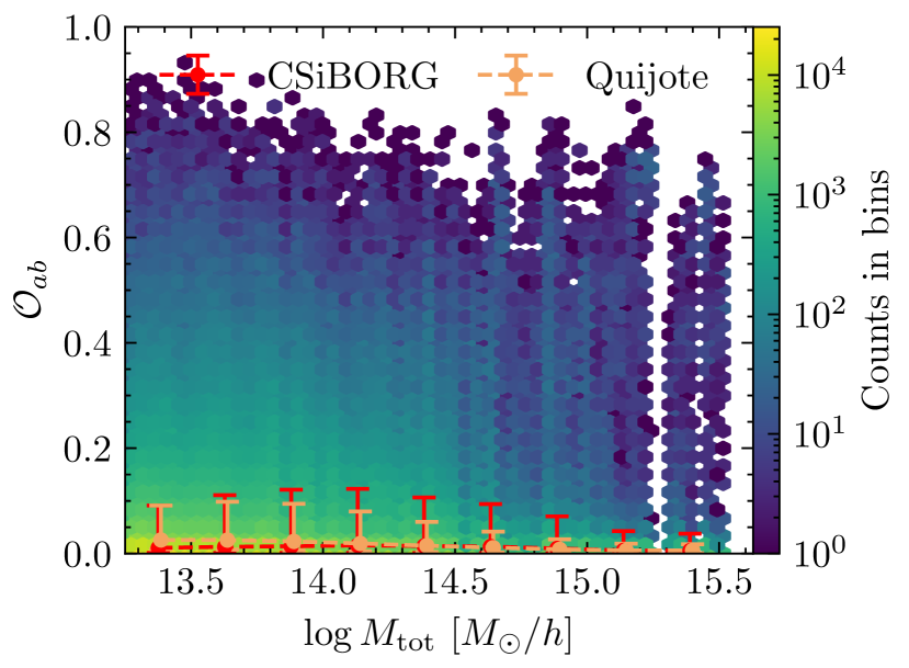
(a) Concatenated pair overlaps $\mathcal{O}_{ab}$ between a reference halo and all haloes from all remaining simulations.

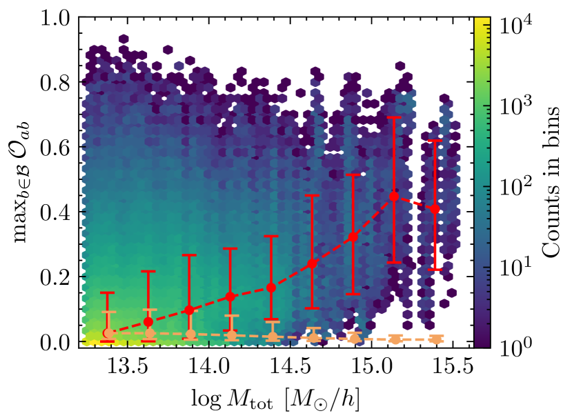
(b) Maximum pair overlaps of a reference halo $\max_{b\in\mathcal{B}}\mathcal{O}_{ab}$ with a single simulation, concatenated across all remaining simulations.

Figure 2: Comparison of Lagrangian patch overlaps in CSIBORG and Quijote simulations. In both cases, a single reference simulation is assumed and for each halo a list of overlaps is calculated per crossing simulation. The $x$-axis denotes the mass of the reference halo, the hex bins illustrate CSIBORG overlaps, with the lines delineating overlaps in CSIBORG and Quijote, each accompanied by $1\sigma$ error bars showing the spread among points. The differentiation in overlap behaviour between the two simulations becomes evident at high mass, where the constraints of the CSIBORG suite become significant.

We showcase the framework on the CSIBORG suite. We first calculate the overlaps of halo initial Lagrangian patches defined in Eq. 3. We then calculate the halo mass, spin and concentration of overlapping haloes and compare them to the reference halo. At each step we compare our findings to the unconstrained Quijote suite to assess the significance of the results. We calculate the overlaps for haloes whose total mass exceeds $10^{13.25}~{}M_{\odot}/h$ and pairs of haloes closer in mass than $2~{}\mathrm{dex}$. This is simply to reduce computational expense, since halo pairs with larger differences in mass have negligible overlaps ($\lesssim 1$ per cent).

4.1 Overlaps

We begin by using a single reference simulation and assessing how consistently its haloes are present in the remaining IC realisations. We calculate the non-zero overlaps between its haloes and those of another simulation following the approach of Section 3. This yields for each halo in the reference simulation a set of overlaps (which could potentially be empty), but its sum will never exceed $1$ because of the denominator of Eq. 1. Retaining the same reference, the process is reiterated across the remaining IC realisations.

4.1.1 Pair overlap

We present the overlaps between haloes in Fig. 2(a) where for every reference halo, we concatenate all sets of overlaps with the remaining IC realisations. As a comparison, in Fig. 2(a) we also show the overlaps in Quijote where we again use a single reference simulation. The hex-bin shows the CSIBORG results and the lines indicate binned medians and $2\sigma$ spread. It is evident that in both CSIBORG and Quijote the most likely overlap value is close to $0$, which follows from the predominance of non-matched halos in both simulation suites. However, a notable distinction emerges in CSIBORG: there is a pronounced tail of high overlaps, especially evident for haloes above $10^{14}~{}M_{\odot}/h$. These massive haloes have counterparts that occupy the same part of the initial snapshot in the majority of the IC realisations. This is not the case in Quijote, where in fact the high-overlap tail becomes less significant for more massive haloes due to their rarity.

4.1.2 Maximum pair overlap

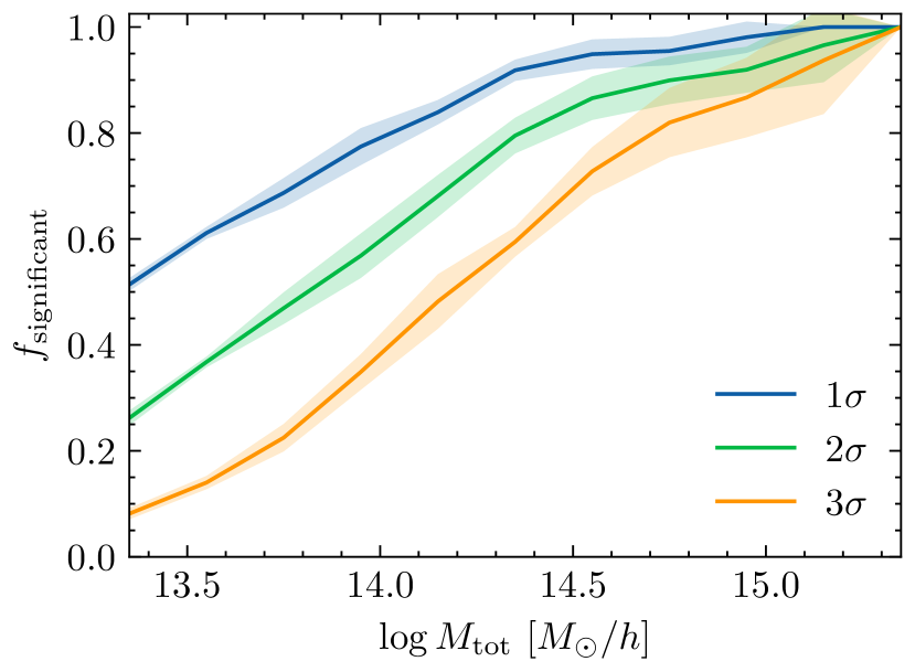
Figure 3: Fraction of CSIBORG reference haloes as a function of $\log M_{\rm tot}$ with median maximum overlap with the remaining IC realisations exceeding the $1,\,2,\,3\sigma$ thresholds in Quijote ($84.1,\,97.7,\,99.9$ per cent). The bands show the $1\sigma$ spread among the CSIBORG realisations. Even at the lower mass threshold a large proportion of CSIBORG haloes has maximum overlaps more significant than in Quijote.

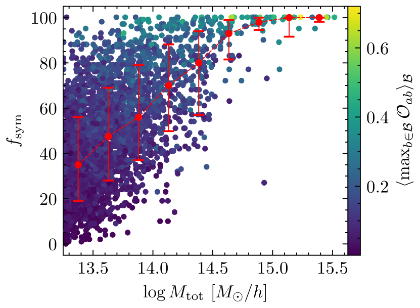
(a) $f_{\rm sym}$ against the reference halo mass.

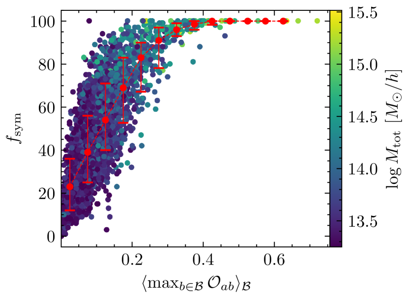
(b) $f_{\rm sym}$ against the average maximum overlap of a halo.

Figure 4: Number of simulations in which a reference halo $a$ and a halo $b$ from a crossing simulation both have maximum overlaps with each other, $f_{\rm sym}$, shown for every halo from a single reference simulation in CSIBORG. The red line is an arithmetic average in a bin along with $1\sigma$ spread. The highest mass haloes have symmetric maximum overlaps in nearly all IC realisations.

Next, we keep the same reference simulation, but instead calculate the maximum overlap of a reference halo in each other IC realisation. In Fig. 2(b) we present the median of the maximum overlaps for each reference halo across the remaining IC realisations. Unlike before, in CSIBORG the mean trend of the maximum overlaps as a function of mass is no longer close to $0$. On the other hand, in Quijote the mean trend of the maximum overlaps remains close to $0$. This indicates that there are halos in any pair of simulation that match well in CSIBORG, especially at high mass, while there are not in Quijote.

In Fig. 3 we show the fraction of CSIBORG haloes in a reference simulation that have a median maximum overlap with other simulations over $1,\,2,\,3\sigma$-level thresholds calculated in Quijote ($84.1,\,97.7,\,99.9$ per cent). This figure again highlights that more massive haloes are more clearly constrained and that already at $10^{14}M_{\odot}/h$ about $75$ per cent of CSIBORG haloes have median maximum overlaps more significant than the $1\sigma$ level in Quijote.

In Fig. 4, we show in CSIBORG for every halo from a single reference simulation the number of simulations in which a reference halo $a$ and a halo $b$ from a crossing simulation both have maximum overlaps with each other ($f_{\rm sym}$). We plot $f_{\rm sym}$ against both the reference halo mass and the average maximum overlap of a halo. On average, haloes around $\sim 10^{14}M_{\odot}/h$ have symmetric maximum overlaps in $50$ per cent of the IC realisations. In contrast, haloes around $\sim 10^{15}M_{\odot}/h$ have symmetric maximum overlaps in nearly all IC realisations. On the other hand, the relationship between $f_{\rm sym}$ and the average maximum overlap has less scatter than its relationship with mass. For example, haloes with an average maximum overlap of $\sim 0.2$ have symmetric maximum overlaps in approximately $50$ per cent of the realisations.

4.1.3 Probability of being matched

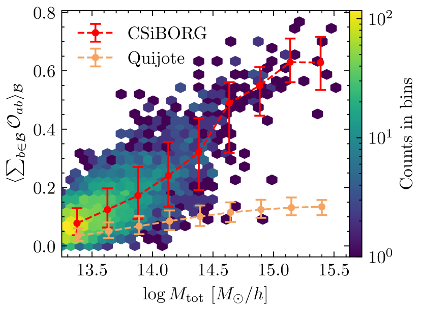
(a) Mean probability of a match averaged over the remaining IC realisations.

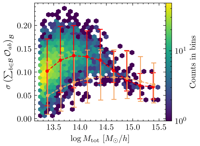
(b) Standard deviation of the probability of a match averaged over the remaining IC realisations.

Figure 5: Probability of a reference halo having a match in the remaining IC realisations calculated as the sum of overlaps. The hex bins show the CSIBORG data and the lines are the mean trends in CSIBORG and Quijote, with $1\sigma$ error bars characterising the spread among points. The probability of a match is typically significantly higher in CSIBORG except for the lower mass threshold where the constraints weaken. The truncation at low masses in Fig. 5(a), and reduction in uncertainty towards very low masses in Fig. 5(b), are due to the lower mass threshold of $10^{13.25}M_{\odot}/h$ when matching halos.

Lastly, we calculate the probability of a reference halo having a counterpart in any other IC realisation, as given by Eq. 4. In Fig. 5 we plot the mean and standard deviation of this probability, averaged over the remaining IC realisations. If a halo has no potential match in another simulation, then the sum of its overlaps in that simulation is simply $0$. Mirroring previous results, there is a clear distinction between CSIBORG and Quijote above $\sim 10^{14}~{}M_{\odot}/h$, in that the majority of CSIBORG halos are matched while the majority of Quijote halos are not. Below this mass, the distinction weakens though it remains significant. The uncertainty on the probability of a match shown in Fig. 5(b) peaks at $10^{14}~{}M_{\odot}/h$. Below this mass, and particularly near the lower mass threshold of $10^{13.25}M_{\odot}/h$, there are only haloes with a mass above this threshold to overlap with, and not below it, thus underestimating the uncertainty.

This is complementary to the results of Fig. 2(b), which was instead sensitive to the maximum overlap a reference halo has with another simulation. On the other hand, in Fig. 5 a high probability of a match can also be due to adding up many small overlaps.

In both CSIBORG and Quijote there is a trend that more massive haloes have higher sum of overlaps, although this is more pronounced in CSIBORG. However, this is not surprising since the most massive haloes have initial Lagrangian patches of $\sim 10~{}\mathrm{Mpc}/h$ and thus are naturally overlapping with more objects. For comparison, see the trend of Fig. 2(b) where the mean trend of the maximum overlaps in Quijote never rises—while the large haloes have overlaps with many small ones such that the sum of overlaps may increase, the maximum overlap a given reference halo has with any one halo in a crossing simulation does not increase with mass.

In Fig. 6 we show in CSIBORG the relation between the probability of being matched and the maximum overlap averaged over the IC realisations. The two quantities are strongly correlated, though the most massive haloes deviate from the $1-1$ line, as smaller overlaps start contribute more significantly to the sum over overlaps. Nevertheless, even for the most massive haloes this shows that sum over overlaps is typically dominated by one object that has a large overlap with the reference halo.

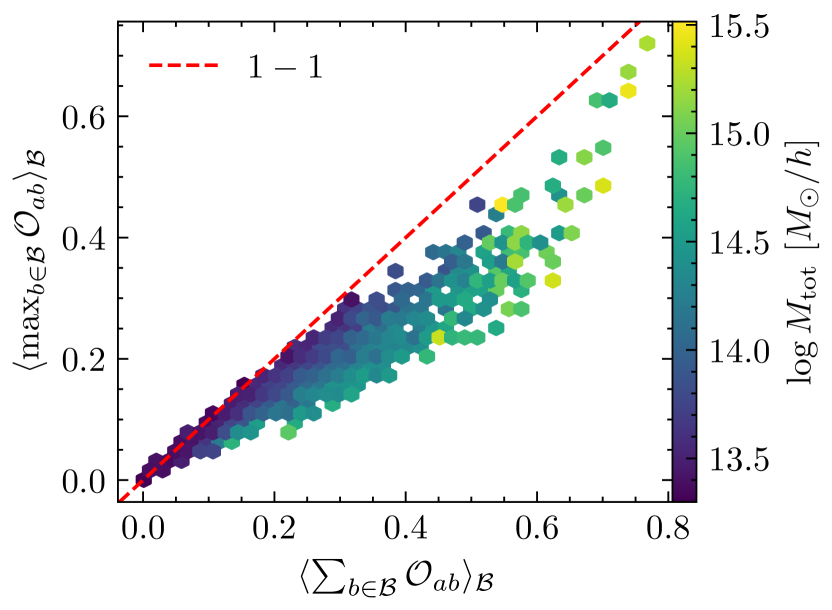
Figure 6: Relation between the mean summed overlap and mean maximum overlap of reference haloes, both of which are averaged over the remaining CSIBORG IC realisations. Although the most massive haloes deviate from the $1-1$ line due to contributions of smaller overlaps, it is clear that the summed overlaps are typically dominated by the overlap to a single object, making the match relatively unambiguous.

4.2 Halo properties of overlapping haloes

Now that we have explored the properties of the overlap statistic and its behaviour across the CSIBORG suite we turn our attention to investigating the properties of halos that it matches. This includes their separation (Section 4.2.1), mass (Section 4.2.2), peculiar velocity (Section 4.2.3) and concentration and spin (Section 4.2.4).

4.2.1 Final snapshot separation of overlapping haloes

For a reference halo that has a significant overlap with a halo in other IC realisation, our anticipation is their proximity in the IC will make the pair unusually close in the final snapshot as well. Because there are nearby halos between boxes even in the absence of any IC constraints, we juxtapose our results with those from the unconstrained Quijote suite. Any suppression in distance observed in CSIBORG relative to Quijote can then be ascribed to the constraints.

We show the results in Fig. 7. We cross-match two IC realisations and compute $\langle\Delta R\rangle$, the overlap-weighted mean separation of haloes in the final snapshot averaged over all IC realisations. In CSIBORG haloes are consistently more likely to remain close in the final snapshot if they originate from the same Lagrangian patch. The lowest mass matched objects in CSIBORG show a variation of $\sim 10~{}\mathrm{Mpc}/h$. For a individual reference haloes and its maximum-overlap matches from the remaining IC realisations we find, as expected, a strong negative correlation between the overlap value and their $z=0$ separation.

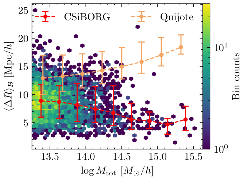
Figure 7: The overlap-weighted mean separation of haloes in the final snapshot $\Delta R$ of CSIBORG realisation $7444$ averaged over all remaining IC realisations. The hex bins are the CSIBORG overlaps and the lines are the CSIBORG and Quijote mean trends, respectively, with $1\sigma$ spread among points Although the halo positions are constrained across the entire mass range when compared to Quijote, there is a significant variation in the positions of the lower mass objects.

4.2.2 Mass of matched haloes

The next quantity that we look at is the most probable mass of the matched haloes. We calculate this following the approach outlined at the end of Section 3. From each crossing simulation we find the mass of the maximally overlapping halo and construct a weighted histogram, where the weights are the maximum overlaps. We then define the most probable mass as the mode of this distribution, with its uncertainty given by the square root of the overlap-weighted average square of residuals around the mode. We plot an example of this in the left panel of Fig. 8 for the most massive halo in a single CSIBORG realisation, finding the most likely mass to be within $0.2~{}\mathrm{dex}$ of the reference halo mass. This is in part by construction, since the overlap itself is preferentially higher for halos that have a similar mass. However, while the overlap is preferentially higher for haloes of a similar mass, it does not guarantee the objects being a “good” match. If that was the case, then we would find that even in Quijote the mass of matched haloes is on average close to the mass of the reference halo, which it is not.

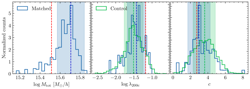
Figure 8: Distributions of most likely matched haloes’ properties ($\log M_{\rm tot}$, $\log\lambda_{\rm 200c}$, $c$) with the most massive halo in one IC realisation (7444) of CSIBORG shown as the blue histogram. The green “control” histogram is the spin and concentration of haloes with a similar mass from the remaining IC realisations: from each we take $10$ haloes closest in mass to the reference halo. The blue and green vertical lines are the mode of the “matched” and “control” histograms, respectively, and the corresponding shaded bands are $1\sigma$ uncertainties. The red line is the reference halo property. A comparison to the control distribution reveals that neither the spin or concentration are constrained. The matched concentration of this halo has a sharp peak near the reference concentration, however a similar trend is not observed for other massive haloes.

By analysing histograms like Fig. 8, we calculate and show in Fig. 9 the most likely mass of all reference haloes in CSIBORG above $10^{13.25}~{}M_{\odot}/h$. In this figure, we show three panels: comparison between the reference and most likely halo mass, the uncertainty of the most likely mass as a function of the reference mass and the ratio of the most likely mass to the reference mass as a function of the median probability of being matched.

The reference and most likely matched halo masses agree well for the most massive objects, with deviations from the $1-1$ line increasing towards lower mass. However, these objects also have a consistently smaller probability of being matched (right panel of Fig. 9) and, therefore it is not unexpected. Below the scale of $\sim 10^{14}~{}M_{\odot}/h$ the matching is less reliable: we only cross-match haloes with mass above $10^{13.25}~{}M_{\odot}/h$ since below this scale the IC constraints weaken as indicated by Fig. 2(b) and Fig. 5(a). Therefore, a reference halo near the threshold will only have potential matches that are above this threshold, thus biasing the matching procedure.

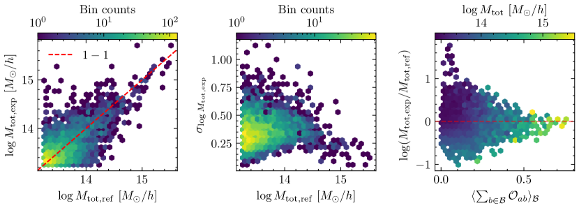
Figure 9: Most likely mass of haloes matched to a single realisation of CSIBORG averaged over all crossing simulations and defined as the mode of a histogram such as Fig. 8. The left panel shows the reference-to-expected halo mass relation, the middle panel shows the uncertainty of the expected mass and the right panel shows the ratio of the expected mass to the reference mass as a function of probability of being matched defined in Eq. 4. The agreement between the reference and matched mass is strongly correlated with the matching probability.

4.2.3 Peculiar velocity alignment

In Fig. 10, we show the alignment and ratio of magnitudes of peculiar velocities in the final snapshot of CSIBORG. We define the alignment angle $\theta$ between the peculiar velocity vectors of haloes $a$ and $b$ with peculiar velocities $\bm{v}_{a}$ and $\bm{v}_{b}$, respectively, as:

$$\cos\theta=\frac{\bm{v}_{a}\cdot\bm{v}_{b}}{|\bm{v}_{a}|~{}|\bm{v}_{b}|}.$$ (6)

For each reference halo we calculate the alignment of its peculiar velocity vector with the corresponding vector of the highest overlapping halo from another IC realisation. We find the alignment of a reference halo and a single maximum overlap crossing halo to be strongly correlated with the magnitude of this overlap across the IC realisations. The alignment and ratio of magnitudes plotted in Fig. 10 is averaged over the crossing IC realisations. While most matched cluster-mass haloes show strong alignment in the final snapshot, there are exceptions. These often coincide with a lower mean maximum overlap. Nevertheless, even plotting the alignment as a function of the mean maximum overlap there remains a significant scatter. We also compare the magnitudes of peculiar velocities, finding their ratios to be on average $\sim 1$, however with significantly larger scatter towards smaller overlaps.

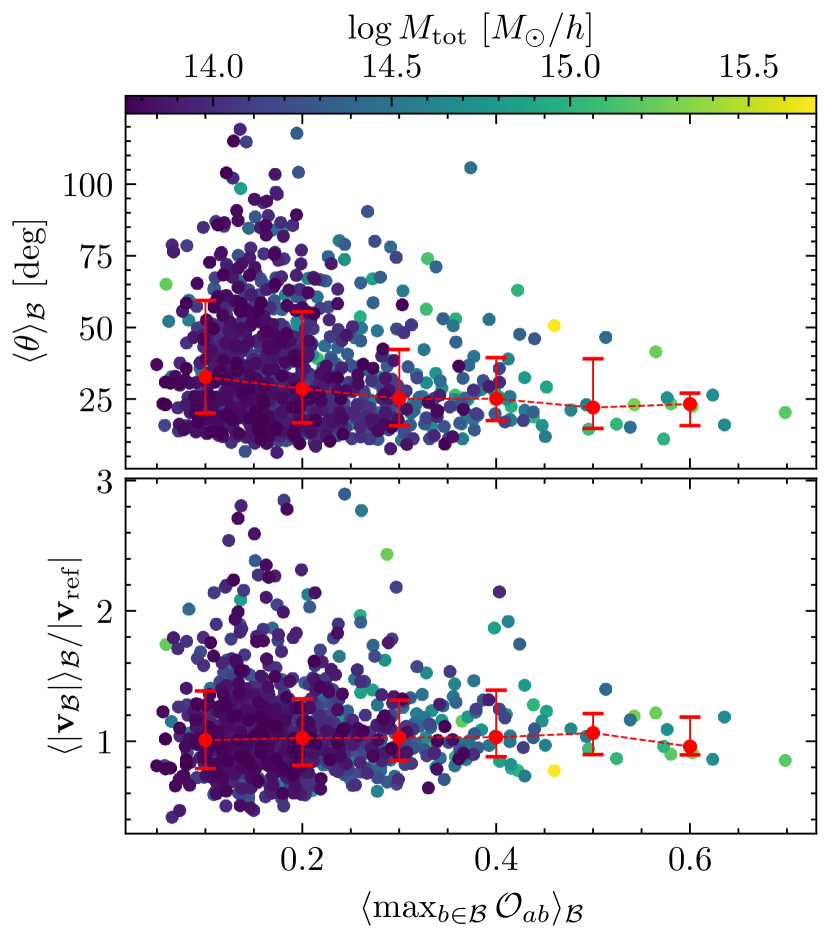
Figure 10: The mean alignment angle (top panel) and ratio of magnitudes (bottom panel) of reference haloes with the remaining IC realisations in CSIBORG, plotted as a function of the mean maximum overlap of the reference halo averaged over the IC realisations. The red line is the mean trend in a bin with $1\sigma$ spread among points. Higher overlapping haloes tend to have their peculiar velocities more aligned in final snapshot.

4.2.4 Spin and concentration constraint

Lastly, we turn our attention to the spin and concentration of these haloes. We use the Bullock spin definition

$$\lambda_{\rm 200c}=\frac{J_{\rm 200c}}{\sqrt{2}M_{\rm 200c}V_{\rm 200c}R_{\rm 200c}},$$ (7)

where $J_{\rm 200c}$ is the angular momentum magnitude of particles within $R_{\rm 200c}$ and $V_{\rm 200c}^{2}=GM_{\rm 200c}/R_{\rm 200c}$ (Bullock et al., 2001). We define the concentration as the ratio of the virial radius to the scale radius of the Navarro-Frenk-White (NFW) profile, $c=R_{\rm 200c}/R_{\rm s}$ (Navarro et al., 1996).

We calculate the most likely spin and concentration of the matched haloes following the approach outlined in Section 3. In the middle panel of Fig. 8 we show the comparison of the spins of overlapping haloes to the spin of a reference halo, which we take to be the most massive halo in one IC realisations of CSIBORG. However, unlike previously we do not find any preference for the spin of overlapping haloes to be similar to the reference halo spin, regardless of whether we weight the matched haloes by overlap or not. The matched distribution in Fig. 8 has a secondary peak near the reference spin, however it is not statistically significant. In fact, the distribution of matched spins is in good agreement with the simulation average, which is approximately a mass-independent Gaussian distribution in $\log\lambda_{\rm 200c}$. We find similar conclusions to hold for all haloes, regardless of their mass.

Next, we investigate the concentration of the matched haloes. In the right panel of Fig. 8 we show the comparison of the concentrations of overlapping haloes to the concentration of a reference halo, which we again take to be the most massive halo in one IC realisations of CSIBORG. We find that in this particular example, the mode of the weighted distribution agrees well with the reference halo concentration but still the width of this distribution is similar to the expectation from the simulated mass–concentration relation. To delve deeper, we assess the matched concentrations for all haloes with a mass exceeding $10^{15}~{}M_{\odot}/h$, which we previously identified as being consistently reconstructed. We find no discernible correlation between the most likely and reference concentrations. We also find that the concentration of the highest overlap halo from each IC realisation is within $10$ ($30$) per cent of the reference value in only $20$ ($50$) per cent of realisations, without any clear dependence on the reference halo mass. The agreement seen in Fig. 8 is thus either coincidental or specific to the halo in question. However, even in such instances, the significance is questionable as there is no notable improvement over the mass–concentration relation.

5 Discussion

5.1 Interpretation of the results

Constrained simulations enable an object-by-object comparison of the local Universe with theory. If a direct, or at least probabilistic, correspondence between a simulated halo and an observed structure can be established, constrained simulations allow inference of the properties and assembly histories of nearby objects and hence pose rigorous tests for galaxy formation models and cosmology. In this work, we outline and test a method for assessing whether a halo is robustly reconstructed across a set of simulations, differing for example in IC drawn from the posterior of a preceding inference. This allows us to compare the properties of “same” halos across the simulations.

We illustrate our framework by applying it to the CSIBORG suite of $101$ constrained simulations of the local $\sim 155~{}\mathrm{Mpc}/h$ Universe with IC on a grid of spacing $2.65~{}\mathrm{Mpc}/h$ derived from the BORG inference of the $\mathrm{2M}\texttt{++}$ catalogue. We find that cluster-mass halos ($M\gtrsim 10^{14}~{}M_{\odot}/h$) are consistently reconstructed across the suite and originate from the same Lagrangian region. Halos of this mass are distributed over $\sim 70$ cells in the initial snapshot at $z=69$. Assuming that the comoving cell density in the initial snapshot is $\Omega_{\rm m}\rho_{\rm c}$, where $\rho_{\rm c}$ is the current critical density of the Universe, we can approximate the spatial resolution, $L$, required to distribute a mass $M$ over $N$ cells as:

$$L\approx 2.6~{}\mathrm{Mpc}/h\left(\frac{M}{10^{14}~{}M_{\odot}/h}\frac{70}{N}\right)^{1/3}.$$ (8)

Assuming the criterion of $70$ resolution elements across the initial Lagrangian patch to be universal, this suggests that for haloes of mass $10^{15},\,10^{14},\,10^{13}~{}M_{\odot}/h$ to be robustly reconstructed one must use IC constraints at the scale $5.5,\,2.6$ and $1.2~{}\mathrm{Mpc}/h$, respectively.

While high-mass haloes are consistently reconstructed and have counterparts of similar mass and peculiar velocity across all IC realisations, the overlapping haloes originating from same Lagrangian regions are not similar in neither their spin or concentration. Despite the BORG reconstruction employed in this work not utilising a peculiar velocity catalogue as a constraint—relying solely on galaxy positions in the $\mathrm{2M}\texttt{++}$ catalogue—it is reassuring to find that the highest mass haloes indeed have aligned velocities, since to some extent galaxy positions are complementary to the peculiar velocity field information. In fact, BORG has been used in the past to reconstruct the local peculiar velocity field (Jasche & Lavaux, 2019).

Cadiou et al. (2021) demonstrated that the angular momentum of haloes can be accurately predicted directly from their Lagrangian patches, but that it exhibits chaotic behaviour under small changes to the patch boundary. Although the high-mass CSIBORG haloes are present in all IC realisations, their overlaps never reach unity and so their Lagrangian patches are not exactly aligned. Therefore, given the findings of Cadiou et al., the lack of constraint on spin is not surprising. The halo concentration depends on both the Lagrangian patch configuration and subsequent accretion history (Rey et al., 2019). While we find that on average the halo concentration in CSIBORG is not constrained, we leave a detailed examination of specific observed clusters for future work along with comparing the mass accretion histories of haloes that are initially strongly overlapping. This will help tease out the properties of halos and their constituent particles that are responsible for setting their concentrations.

For certain haloes, we observe that those originating from consecutive CSIBORG simulations tend to have higher maximum overlaps. CSIBORG resimulates every $24$^th step of the BORG chain, yet the auto-correlation length of the chain is $\sim 100$. CSIBORG thus effectively over-samples the BORG posterior—even though it varies without correlation the unconstrained small-scale modes at each step—which could lead to an overestimation of confidence in the BORG constraints if relying only on a few consecutive CSIBORG samples. To mitigate this effect we have averaged across all remaining $100$ IC realisations for each reference realisation, the majority of which are fully decorrelated from it. A fully satisfactory solution would be to resimulate only decorrelated IC realisations, however it is challenging to derive a large number of these due to the high computational cost of the BORG inference.

5.2 Comparison with the literature

Hutt et al. (2022) introduce an algorithm for assessing whether “twins” of a single halo can be identified in all IC realisations of a constrained simulation. This is done by selecting a reference simulation and cataloguing the positions of all haloes. A halo is then chosen from the reference simulation, and its size calculated as $R_{\rm 200c}=\left[(3M_{\rm 200c})/(4\pi\cdot 200\cdot\rho_{\rm crit})\right]^{1/3}$. In the other simulations, haloes within a designated “search radius” of the reference halo are then identified and the one most similar in mass selected. If no haloes are found within the search radius, the reference halo is discarded as not present within the crossing simulation. This approach differs from ours in several important ways:

1. we match haloes directly in the IC, which are constrained by BORG, instead of relying on the forward-modelled realisations of the final snapshot,

2. we do not require the matched haloes to be within a fixed radius of one another, but instead calculate the overlap of their initial Lagrangian patches,

3. while the procedure of Hutt et al. is inherently binary, ours has a continuous interpretation in terms of probabilities.

It is nevertheless instructive to compare our results. In Fig. 11 we show the fraction of matches identified via the approach of Hutt et al. that are also the maximum-overlap pairs for several choices of search radii in CSIBORG. Because of the stringent requirement of Hutt et al. that a halo must have a “twin” in all IC realisations, there is a strong agreement between the two approaches. We calculate $f_{\rm agreement}$, the fraction of matches identified by Hutt et al. that are also the maximum-overlap pairs as a function of a lower mass threshold. For the fiducial search radius used by Hutt et al. the agreement is $\sim 90$ per cent regardless of the mass threshold. This does, however, come at the cost of only a small number of haloes being identified as matches by Hutt et al.: for example at $10^{14}~{}M_{\odot}/h$ this is only $\sim 10$ per cent of the haloes. Our method has the advantage of providing useful information even in the regime where the matching across all realisations is partial or even weak.

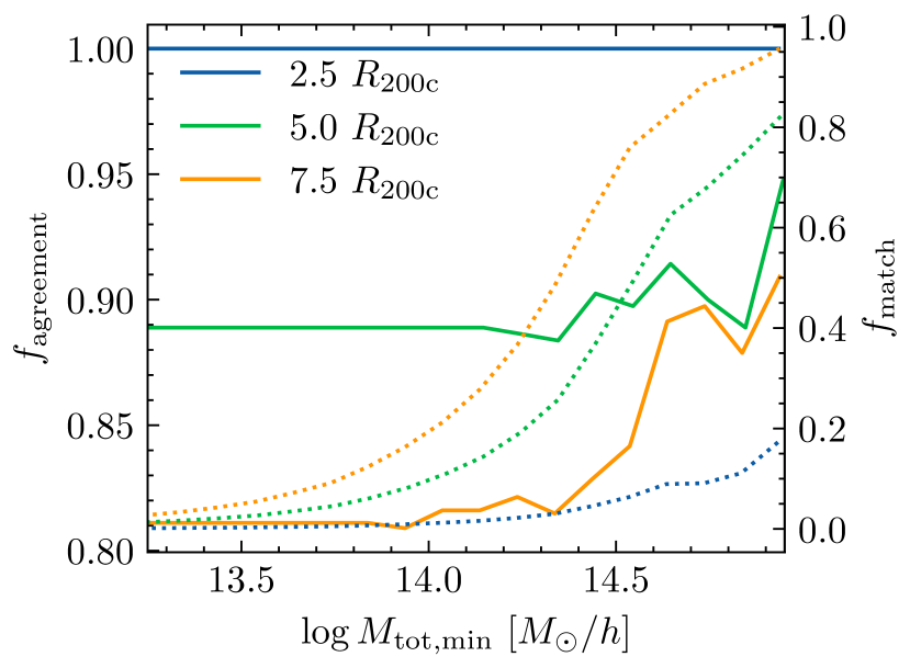
Figure 11: Comparison of our matching procedure to that of Hutt et al. (2022), who identify “twin” halos in the final snapshots of CSIBORG. Solid lines correspond to $f_{\rm agreement}$, which is the fractional agreement between the Hutt et al. matches and the maximum-overlap pairs above mass $M_{\rm tot,min}$. Dotted lines are $f_{\rm match}$, the fraction of haloes above $M_{\rm tot,min}$ identified as matches by Hutt et al.. The high $f_{\rm agreement}$ indicates excellent agreement between the approaches regardless of the search radius (shown in the legend). However, only a small fraction of halos are identified as matches by Hutt et al.. Our method establishes a match probability applicable even to far more uncertain matches.

Another methodology with similarities to ours is that of Pfeifer et al. (2023), in which the goal is to identify the simulation most representative of the local Universe. They use a Wiener filter-based reconstruction that must be supplied with random small scale/unconstrained modes. This strategy can alternatively be conceptualised as an intensive fine-tuning process to pinpoint the optimal random seed on a very fine grid level, which can be then re-simulated (McAlpine et al., 2022). Pfeifer et al. find the realisation that best resembles the local Universe by minimizing the sum of $p$-values of simulated cluster-mass haloes being at the locations of observed clusters. However, while they find the most representative constrained simulations, their approach does not provide any information about the consistency with which the matched simulated haloes are reconstructed. We believe that this is crucial information to determine the confidence with which we can assert the properties of the dark matter distribution of the local Universe, given the quality and quantity of data used to set the constraints.

A similar technique of matching observed galaxies to haloes from constrained cosmological simulations has been applied by Zhang et al. (2022); Xu et al. (2023). Zhang et al. develop a “neighbourhood” SHAM, a SHAM model specifically tailored for constrained cosmological simulations which ranks haloes based on both their peak mass and closeness in position and velocity to the observed galaxy (Yang et al., 2018). This statistical approach enables them to connect haloes in their single constrained simulation with observed galaxies, thereby facilitating the study of e.g. the galaxy-to-halo size relation. Our method would allow folding in the uncertainties associated with the reconstruction.

6 Conclusion

We have investigated the extent to which halos are robustly reconstructed across multiple cosmological simulations. While this question is particularly pertinent to simulation suites constrained (with uncertainty) to match the local Universe, other applications include the matching of haloes between DM-only simulations and their hydrodynamical counterparts, or simulations of varying cosmology such as $\Lambda\mathrm{CDM}$ vs modified gravity.

We argue that for a halo to be consistently reconstructed its Lagrangian patch in the initial conditions must strongly overlap with a halo in most other realisations of the suite, a condition implying similarity in both mass and location. This is a stricter and more causal measure than similarity in the final snapshot, providing a clearer condition for two halos to be “the same”. In the future, an even stricter measure of similarity may be introduced by measuring the haloes’ initial overlap in the $6\mathrm{D}$ phase space directly, instead of only the $\mathrm{3}\mathrm{D}$ position space.

We apply the method to CSIBORG, a suite of constrained simulations with initial conditions sampled from the posterior of the BORG algorithm applied to the $\mathrm{2M}\texttt{++}$ galaxy number density field. We establish the significance of the results by comparing to the unconstrained Quijote suite. Based on the criteria mentioned above, we find cluster-mass haloes ($M\gtrsim 10^{14}M_{\odot}/h$) to be consistently reconstructed in CSIBORG in position, mass and peculiar velocity, with higher mass haloes being typically more strongly constrained. For haloes below this mass threshold, the constraints diminish, and haloes do not consistently originate from the same Lagrangian patches. Regarding secondary halo properties like spin and concentration, even the consistently matched, high-mass haloes display variations across the IC realisations. The absence of constraints on concentration is surprising, given its strong dependence on both mass and assembly history.

This might imply that the assembly history of even the most massive haloes in CSIBORG remains unconstrained, however we defer a comprehensive study of nearby clusters to future work. In sum, our framework provides a step towards the goal of identifying the IC that led to the observed Universe and the objects it contains.

7 Data availability

The code underlying this article is available at https://github.com/Richard-Sti/csiborgtools and other data will be made available on reasonable request to the authors.

References

- Angulo & Hahn (2022) Angulo R. E., Hahn O., 2022, Living Reviews in Computational Astrophysics, 8, 1
- Bartlett et al. (2021) Bartlett D. J., Desmond H., Ferreira P. G., 2021, Phys. Rev. D, 103, 023523
- Bartlett et al. (2022) Bartlett D. J., Kostić A., Desmond H., Jasche J., Lavaux G., 2022, Phys. Rev. D, 106, 103526
- Bistolas & Hoffman (1998) Bistolas V., Hoffman Y., 1998, ApJ, 492, 439
- Bullock et al. (2001) Bullock J. S., Dekel A., Kolatt T. S., Kravtsov A. V., Klypin A. A., Porciani C., Primack J. R., 2001, ApJ, 555, 240
- Butsky et al. (2016) Butsky I., et al., 2016, MNRAS, 462, 663
- Cadiou et al. (2021) Cadiou C., Pontzen A., Peiris H. V., 2021, MNRAS, 502, 5480
- Cataldi et al. (2021) Cataldi P., Pedrosa S. E., Tissera P. B., Artale M. C., 2021, MNRAS, 501, 5679
- Davis et al. (1985) Davis M., Efstathiou G., Frenk C. S., White S. D. M., 1985, ApJ, 292, 371
- Desmond et al. (2017) Desmond H., Mao Y.-Y., Wechsler R. H., Crain R. A., Schaye J., 2017, MNRAS, 471, L11
- Desmond et al. (2022) Desmond H., Hutt M. L., Devriendt J., Slyz A., 2022, MNRAS, 511, L45
- Diemer & Kravtsov (2015) Diemer B., Kravtsov A. V., 2015, ApJ, 799, 108
- Doumler et al. (2013a) Doumler T., Hoffman Y., Courtois H., Gottlöber S., 2013a, MNRAS, 430, 888
- Doumler et al. (2013b) Doumler T., Gottlöber S., Hoffman Y., Courtois H., 2013b, MNRAS, 430, 912
- Eisenstein & Hut (1998) Eisenstein D. J., Hut P., 1998, ApJ, 498, 137
- Gottloeber et al. (2010) Gottloeber S., Hoffman Y., Yepes G., 2010, arXiv e-prints, p. arXiv:1005.2687
- Griffen et al. (2016) Griffen B. F., Ji A. P., Dooley G. A., Gómez F. A., Vogelsberger M., O’Shea B. W., Frebel A., 2016, ApJ, 818, 10
- Hinshaw et al. (2009) Hinshaw G., et al., 2009, ApJS, 180, 225
- Hoffman & Ribak (1991) Hoffman Y., Ribak E., 1991, ApJ, 380, L5
- Hoffman et al. (2015) Hoffman Y., Courtois H. M., Tully R. B., 2015, MNRAS, 449, 4494
- Hutt et al. (2022) Hutt M. L., Desmond H., Devriendt J., Slyz A., 2022, MNRAS, 516, 3592
- Jasche & Lavaux (2019) Jasche J., Lavaux G., 2019, A&A, 625, A64
- Jasche & Wandelt (2013) Jasche J., Wandelt B. D., 2013, MNRAS, 432, 894
- Jasche et al. (2015) Jasche J., Leclercq F., Wandelt B. D., 2015, J. Cosmology Astropart. Phys., 2015, 036
- Klypin et al. (2003) Klypin A., Hoffman Y., Kravtsov A. V., Gottlöber S., 2003, ApJ, 596, 19
- Knebe et al. (2013) Knebe A., et al., 2013, MNRAS, 435, 1618
- Kolatt et al. (1996) Kolatt T., Dekel A., Ganon G., Willick J. A., 1996, ApJ, 458, 419
- Kostić et al. (2023) Kostić A., Bartlett D. J., Desmond H., 2023, arXiv e-prints, p. arXiv:2304.10301
- Kravtsov et al. (2002) Kravtsov A. V., Klypin A., Hoffman Y., 2002, ApJ, 571, 563
- Lacey & Cole (1993) Lacey C., Cole S., 1993, MNRAS, 262, 627
- Lavaux & Jasche (2016) Lavaux G., Jasche J., 2016, MNRAS, 455, 3169
- Lukić et al. (2009) Lukić Z., Reed D., Habib S., Heitmann K., 2009, ApJ, 692, 217
- McAlpine et al. (2022) McAlpine S., et al., 2022, MNRAS, 512, 5823
- Mitchell et al. (2018) Mitchell P. D., et al., 2018, MNRAS, 474, 492
- Naidoo et al. (2023) Naidoo K., Hellwing W. A., Bilicki M., Libeskind N., Pfeifer S., Hoffman Y., 2023, Phys. Rev. D, 107, 043533
- Navarro et al. (1996) Navarro J. F., Frenk C. S., White S. D. M., 1996, ApJ, 462, 563
- Onions et al. (2012) Onions J., et al., 2012, MNRAS, 423, 1200
- Pallero et al. (2023) Pallero D., Gómez F. A., Padilla N. D., Jaffé Y. L., Baugh C. M., Li B., Hernández-Aguayo C., Arnold C., 2023, arXiv e-prints, p. arXiv:2310.02333
- Pfeifer et al. (2023) Pfeifer S., Valade A., Gottlöber S., Hoffman Y., Libeskind N. I., Hellwing W. A., 2023, Monthly Notices of the Royal Astronomical Society, 523, 5985
- Planck Collaboration et al. (2014) Planck Collaboration et al., 2014, A&A, 571, A1
- Porqueres et al. (2021) Porqueres N., Heavens A., Mortlock D., Lavaux G., 2021, MNRAS, 502, 3035
- Power et al. (2003) Power C., Navarro J. F., Jenkins A., Frenk C. S., White S. D. M., Springel V., Stadel J., Quinn T., 2003, MNRAS, 338, 14
- Press & Schechter (1974) Press W. H., Schechter P., 1974, ApJ, 187, 425
- Prideaux-Ghee et al. (2023) Prideaux-Ghee J., Leclercq F., Lavaux G., Heavens A., Jasche J., 2023, MNRAS, 518, 4191
- Rey et al. (2019) Rey M. P., Pontzen A., Saintonge A., 2019, MNRAS, 485, 1906
- Sawala et al. (2022) Sawala T., McAlpine S., Jasche J., Lavaux G., Jenkins A., Johansson P. H., Frenk C. S., 2022, MNRAS, 509, 1432
- Skrutskie et al. (2006) Skrutskie M. F., et al., 2006, AJ, 131, 1163
- Sorce et al. (2016) Sorce J. G., et al., 2016, MNRAS, 455, 2078
- Springel et al. (2008) Springel V., et al., 2008, MNRAS, 391, 1685
- Stopyra et al. (2021) Stopyra S., Peiris H. V., Pontzen A., Jasche J., Natarajan P., 2021, MNRAS, 507, 5425
- Stopyra et al. (2023) Stopyra S., Peiris H. V., Pontzen A., Jasche J., Lavaux G., 2023, arXiv e-prints, p. arXiv:2304.09193
- Tassev et al. (2013) Tassev S., Zaldarriaga M., Eisenstein D. J., 2013, J. Cosmology Astropart. Phys., 2013, 036
- Teyssier (2002) Teyssier R., 2002, A&A, 385, 337
- Tinker et al. (2008) Tinker J., Kravtsov A. V., Klypin A., Abazajian K., Warren M., Yepes G., Gottlöber S., Holz D. E., 2008, ApJ, 688, 709
- Valade et al. (2022) Valade A., Hoffman Y., Libeskind N. I., Graziani R., 2022, MNRAS, 513, 5148
- Valade et al. (2023) Valade A., Libeskind N. I., Hoffman Y., Pfeifer S., 2023, MNRAS, 519, 2981
- Villaescusa-Navarro et al. (2020) Villaescusa-Navarro F., et al., 2020, ApJS, 250, 2
- Vogelsberger et al. (2020) Vogelsberger M., Marinacci F., Torrey P., Puchwein E., 2020, Nature Reviews Physics, 2, 42
- Wang et al. (2014) Wang H., Mo H. J., Yang X., Jing Y. P., Lin W. P., 2014, ApJ, 794, 94
- Wang et al. (2016) Wang H., et al., 2016, ApJ, 831, 164
- Warren et al. (2006) Warren M. S., Abazajian K., Holz D. E., Teodoro L., 2006, ApJ, 646, 881
- Wechsler & Tinker (2018) Wechsler R. H., Tinker J. L., 2018, ARA&A, 56, 435
- Xu et al. (2023) Xu X., Yang X., Xu H., Zhang Y., 2023, arXiv e-prints, p. arXiv:2307.00060
- Yang et al. (2018) Yang X., et al., 2018, ApJ, 860, 30
- Zaroubi et al. (1995) Zaroubi S., Hoffman Y., Fisher K. B., Lahav O., 1995, ApJ, 449, 446
- Zaroubi et al. (1999) Zaroubi S., Hoffman Y., Dekel A., 1999, ApJ, 520, 413
- Zhang et al. (2022) Zhang Y., Yang X., Guo H., 2022, MNRAS, 517, 3579
- van de Weygaert & Hoffman (2000) van de Weygaert R., Hoffman Y., 2000, in Courteau S., Willick J., eds, Astronomical Society of the Pacific Conference Series Vol. 201, Cosmic Flows Workshop. p. 169 (arXiv:astro-ph/9909103), doi:10.48550/arXiv.astro-ph/9909103
- van den Bosch & Jiang (2016) van den Bosch F. C., Jiang F., 2016, MNRAS, 458, 2870
- van den Bosch & Ogiya (2018) van den Bosch F. C., Ogiya G., 2018, MNRAS, 475, 4066