The effect of demographic stochasticity on predatory-prey oscillations

Abstract

The ecological dynamics of interacting predator and prey populations can display sustained oscillations, as for instance predicted by the Rosenzweig-MacArthur predator-prey model. The presence of demographic stochasticity, due to the finiteness of population sizes, alters the amplitude and frequency of these oscillations. Here we present a method for characterizing the effects of demographic stochasticity on the limit cycle attractor of the Rosenzweig-MacArthur. We show that an angular Brownian motion well describes the frequency oscillations. In the vicinity of the bifurcation point, we obtain an analytical approximation for the angular diffusion constant. This approximation accurately captures the effect of demographic stochasticity across parameter values.

I Introduction

The independent works of Alfred Lotka and Vito Volterra [1, 2] showed more than 100 years ago how predator-prey population dynamics can display neutral oscillation (where the amplitude depends on the initial condition) with a fixed frequency. The extension of their models by Rosenzweig and MacArthur [3] — formulated to include more realistic, i.e., saturating, functional responses — gives rise, in some parameter regimes, to stable limit cycles: prey and predator populations converge to oscillations with fixed frequency and amplitude, independent of the initial condition. Population oscillations have been observed in natural predator–prey ecosystems and confirmed by experiments [4, 5, 6, 7, 8, 9], even if it is debated whether their origin is endogenous (as predicted by the Rosenzweig-MacArthur (RMA) model) or exogenous (e.g. due to environmental fluctuations).

In reality, population dynamics are generally stochastic, due to intrinsic or extrinsic reasons. Extrinsic reasons include environmental fluctuations, such as weather, fires, seasonality as well as biotic disturbances [10, 11]. Intrinsic reasons are demographic effects of the discrete nature of the population: birth, death, and migrations are individual processes occurring randomly — and independently across individuals — with some rates. Due to their independence across individuals, these random demographic effects become negligible for very large population sizes, and the deterministic limit is recovered.

Demographic stochasticity can strongly affect the dynamical attractor in presence of non-linearities. For example, even in simple predator-prey systems, quasi cycles may appear as a result of demographic noise, while the deterministic solution is a stable fixed point [12]. In presence of limit cycle, demographic noise can affect both amplitude and phase.

In this paper, we study a non-linearly coupled predator-prey system, the Rosenzweig-MacArthur model, which is a generalization of Lotka-Volterra model with a Holling type II functional response [13]. In some parameters regime, the Rosenzweig-MacArthur model has a globally attractive limit cycle. In this paper, we focus on the effect of demographic stochasticity on the limit cycle trajectories, with the goal of understanding quantitatively how amplitude, frequency, and phase are affected.

This paper is organized as follows: in section II, we introduce the deterministic and stochastic Rosenzweig-MacArthur model. In Section III, we present our results in three different subsections. First, we give an analytical approximation to find the mean frequency and the radius of the limit cycle close to the bifurcation point. Next, we show that the perturbations along the limit cycle can be approximated by an angular Brownian motion. Then, we extract an analytic expression for the noise strength using Van Kampen system size expansion of the corresponding Fokker-Planck equation. Finally, a brief summary and some concluding remarks are presented in section IV.

II The Rosenzweig-MacArthur Predator-Prey Model

The Rosenzweig-MacArthur Predator-Prey Model [3] provides a standard framework to study the coupled dynamics of predator and prey populations. The population abundances of the prey ($R$) and predators ($F$) change in time accordingly to

$$\dot{R}=aR-\dfrac{R^{2}}{2N}-\dfrac{sRF}{1+s\tau R},$$

$$\dot{F}=-dF+\dfrac{sRF}{1+s\tau R}\ .$$ (1)

In the absence of predators ($F=0$), the preys grow logistically, with growth rate $a$ and carrying capacity $2Na$. In the absence of preys ($R=0$) the predator population declines with death rate $d$. The per-capita predation rate has a Holling type II functional response which saturates to $1/\tau$ for large predator populations. The base predation rate equals to $s$.

Without loss of generality, we define $d=1$ (which corresponds to set a global timescale) and set population abundances $x=R/N$ and $y=F/N$ to obtain

$$\dot{x}=ax-\dfrac{x^{2}}{2}-\dfrac{\sigma xy}{1+\sigma\tau x},$$

$$\dot{y}=-y+\dfrac{\sigma xy}{1+\sigma\tau x}\ ,$$ (2)

where $\sigma=sN$. In the previous studies [3, 14, 15], people have shown that when:

$$0<\tau<1,$$

$$\sigma>\sigma_{0}=\dfrac{1}{2a(1-\tau)},$$ (3)

equation 2 has three distinct fixed points:

$$M_{1}=(x=0,y=0),$$

$$M_{2}=(x=2a,y=0),$$

$$M_{3}=(x=\dfrac{1}{\sigma(1-\tau)},y=\dfrac{2a\sigma(1-\tau)-1}{2\sigma^{2}(1-\tau)^{2}})\ .$$ (4)

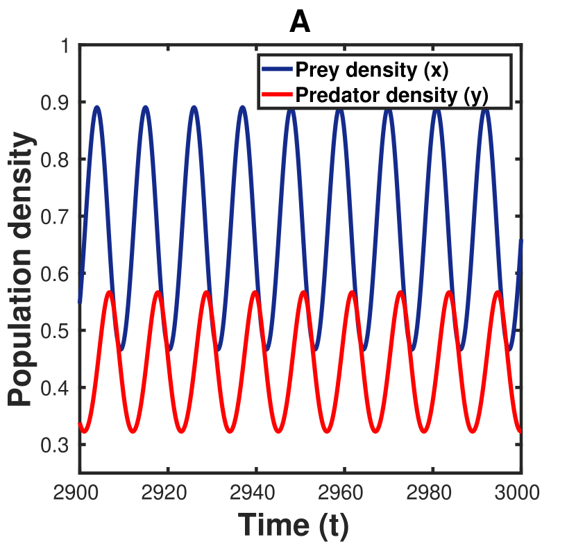
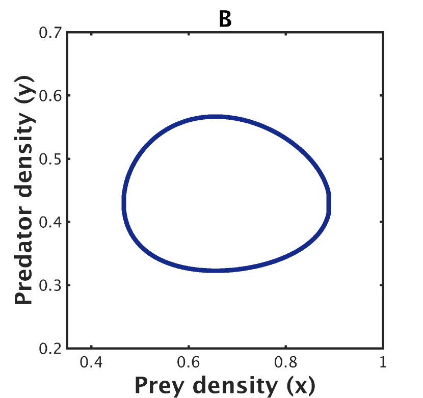
The trivial fixed point $M_{1}$ is corresponding to extinction of both species. It is a saddle point: attracting in the y direction and repelling in the x direction. $M_{2}$ corresponds to the state that only the prey is present, and it is also a saddle point: attracting in the x direction, but repelling in a direction corresponding to the introduction of a few predators into the system. Predator and prey coexists with fixed point $M_{3}$ which is stable, when $\sigma_{0}<\sigma<\sigma^{*}=\dfrac{1+\tau}{2a\tau(1-\tau)}$. For $\sigma>\sigma^{*}$, $M_{3}$ is an unstable node where the dynamics converges to a stable limit cycle as depicted in figure 1.

The deterministic model can be generalized to include stochasticity by considering discrete number of individuals $F$ and $R$, which change with the following rates:

$$T(F,R+1|R,F)=aR,$$

$$T(F+1,R-1|R,F)=\dfrac{sRF}{1+s\tau R},$$

$$T(F,R-1|R,F)=\dfrac{R^{2}}{2N},$$

$$T(F-1,R|R,F)=F,$$ (5)

where $T(C_{f}|C_{i})$ indicates the rate from initial configuration $C_{i}$ to final configuration $C_{f}$.

These rates fully define the stochastic process determining the dynamics of the system [3, 15], that, in the limit of $N\to\infty$, can be approximated with eq. 2. We implemented the Gillespie algorithm [16] to numerically simulate the stochastic RMA system. In this algorithm, the time step to the next event and the next event itself, are chosen randomly.

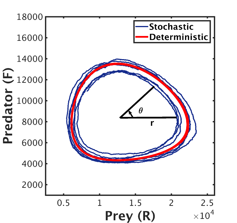
Figure 2 displays one stochastic trajectory of the RMA system, in the parameter regime where a limit cycle in the deterministic system is expected. While the trajectories are noisy, they still resemble the deterministic limit cycle.

Figure 1: Deterministic and Stochastic RMA model. (A) Oscillations of populations versus time, where blue and red correspond to prey and predator densities respectively. (B) The corresponding limit cycle in phase space. Parameters in these figures are $\tau=0.5$, $a=1$ and $\sigma=3.05$.

Figure 2: Limit cycles of the deterministic and Stochastic RMA models. Radius ($r$) and phase ($\theta$) in the phase space has been determined in the figure. Deterministic limit cycle has been distinguished by red color. Parameters in these figures are $\tau=0.5$, $a=1$, $N=20000$ and $\sigma=3.2$.

III Results

In the previous section, we provided the definition of the deterministic and stochastic RMA model. In the parameter regime where a limit cycle occurs, the stochastic trajectory still displays an oscillatory behavior. In this section, we linearize the fluctuations around the deterministic attractor and quantify the effect of stochasticity. We then compare the analytical results with numerical simulations.

III.1 Elliptical Approximation of the Limit Cycle

In order to quantify the noise strength along the limit cycle, we need to rewrite the differential equations in the polar phase space. We can approximate the shape of the limit cycle to an ellipse, when the amplitude of the oscillations is small. In particular, this occurs when the parameter $\sigma/\sigma^{*}\to 1^{+}$, and in that case the oscillations occur in the vicinity of the $M_{3}$. It is convenient to introduce $\gamma=\dfrac{\sigma-\sigma^{*}}{\sigma^{*}}$. Our approximation holds for small and positive values of $\gamma$. To this end, we will define $dx$ and $dy$ as follows:

$$dx=r(t)\cos\theta(t),$$

$$dy=r(t)\epsilon\sin\theta(t),$$ (6)

where $dx=(x-x_{f})$, $dy=(y-y_{f})$ and $(x_{f},y_{f})$ is the coordinates of the $M_{3}$ in the phase space. The variable $\theta$ is the phase variable on the limit cycle centered at the mentioned fixed point ($M_{3}$), which is calculated as follows:

$$\theta=tan^{-1}(\dfrac{y-y_{f}}{x-x_{f}}).$$ (7)

The phase value goes from $0$ to $2\pi$ as the system evolves by time and completes a cycle in the phase-space, as illustrated in Figure 2. By expanding the equation 2 around $(x_{f},y_{f})$ and using equation 6, one can find $\dot{r}$ and $\dot{\theta}$ (see details in the supplementary materials). Under this approximation, one obtains the mean frequency ($\omega$) and the mean radius ($\left\langle r\right\rangle$) that read:

$$\omega=\epsilon=\sqrt{a(1-\tau)-\dfrac{1}{2\sigma}},$$

$$\left\langle r\right\rangle=\dfrac{2a\sqrt{\dfrac{\gamma\tau(1+\tau)}{1+\gamma-\tau+\gamma\tau}}}{1+\gamma+\tau+\gamma\tau}\ .$$ (8)

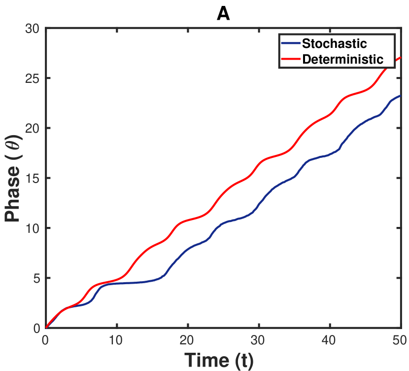
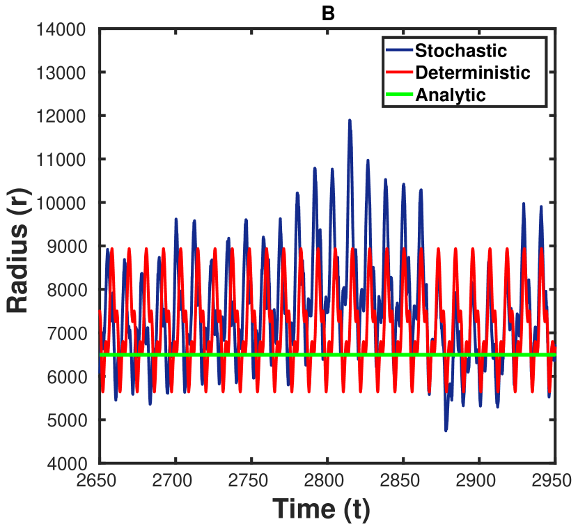
We provide a confirmation of the analytical results using direct numerical simulation of the deterministic and discrete simulation of stochastic RMA models. Figure 3 shows time evolution of the phase and radius of limit cycle for deterministic and stochastic RMA model. Our analytical approximation for mean radius is in agreement with the simulation results.

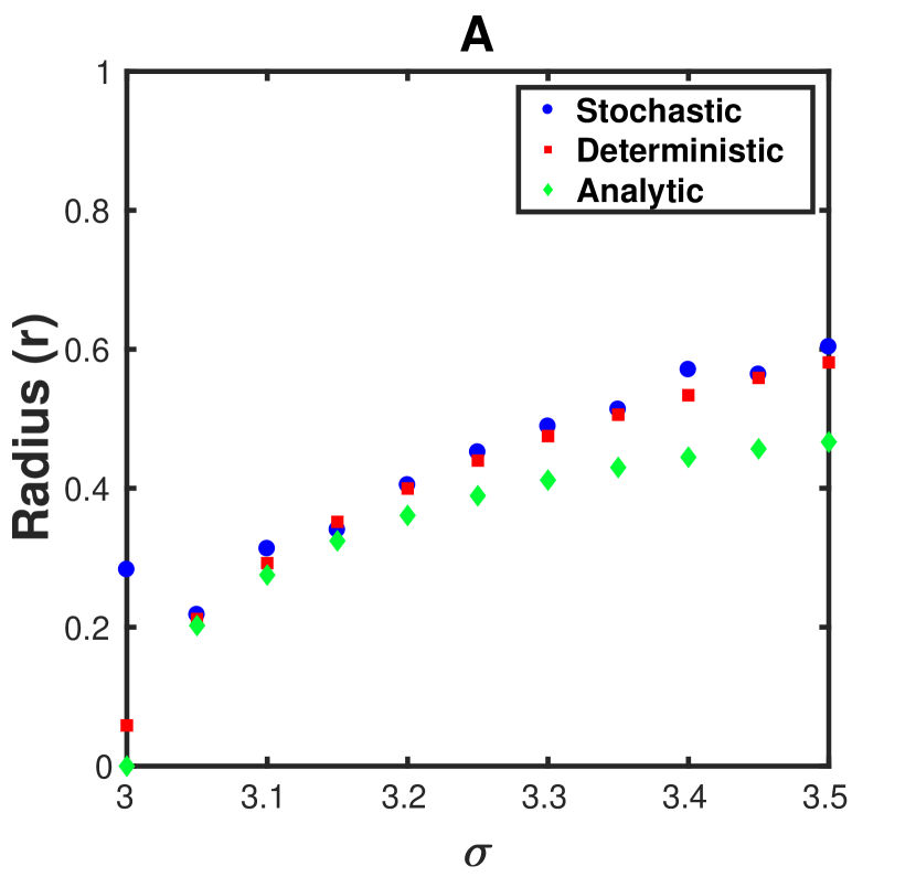
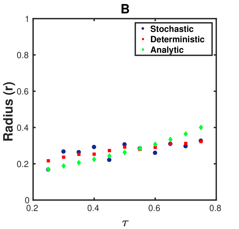
Figure 4 illustrates the dependency of the mean radius ($\left\langle r\right\rangle$) versus system parameters $\tau$ and $\sigma$ obtained using stochastic simulation and analytical approximation. One can see that the obtained results are in agreement when we are close to the fixed point $M_{3}$ ($0<\gamma=\dfrac{\sigma-\sigma^{*}}{\sigma^{*}}\leqslant 0.15$). As the amplitude of the limit cycle increases (i.e., when we increase the value of $\gamma$) the approximation become less and less accurate. This mismatch occurs because the shape of the limit cycle becomes more and more different from an ellipse.

Figure 3: Comparison of deterministic, stochastic and analytic approximation of RMA model. (A) Phase versus time (N = 1800). (B) Radius versus time (N = 20000). Parameters in these figures are $\tau=0.5$, $a=1$ and $\sigma=3.2$.

Figure 4: Comparison of stochastic, deterministic, and analytical radius values versus different model parameters. Parameters are $\gamma=0.06$, $a=1$, $\tau=0.5$ and $N=25000$.

III.2 Angular Brownian Motion and The Noise Strength

Demographic stochasticity affects the trajectory in two ways: first, it produces fluctuations in the amplitude and secondly, it determines fluctuations in the phase of these oscillations. In this work, we mostly focus on the latter. In that context, it is natural to approximate the phase trajectory as an angular Brownian motion [17], with fixed frequency (corresponding to the one of eq. 8), and as angular diffusion term, with diffusion constant $D$. This ansatz is consistent with the results of figure 2, where the time evolution of the phase oscillates around a constant frequency. Therefore, the corresponding Langevin equation [17] for the angular position $\theta$ can be written as follows:

$$\dot{\theta}=\omega+\sqrt{D}\xi(t)\ ,$$ (9)

where $D$ is the diffusion constant and $\xi(t)$ is a white, delta correlated, Gaussian noise.

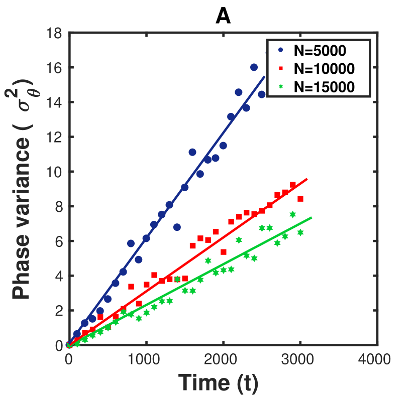
Eq. 9 predicts that the variance of $\theta$ (calculated across independent realizations of the process starting from the same initial conditions) grows at $Dt$. Figure 5 shows that, in agreement with the Geometric Brownian Motion ansatz, the variance of the phase increase linearly with time.

The diffusion constant $D$ plays therefore the role of an effective parameter, capturing the effect of stochasticity on the limit cycle trajectories. Our goal is to determine, in the linear noise approximation, the dependency of this effective diffusivity $D$ on the parameters of the RMA model ($a$, $\sigma$, and $\tau$) as well as on the population size $N$.

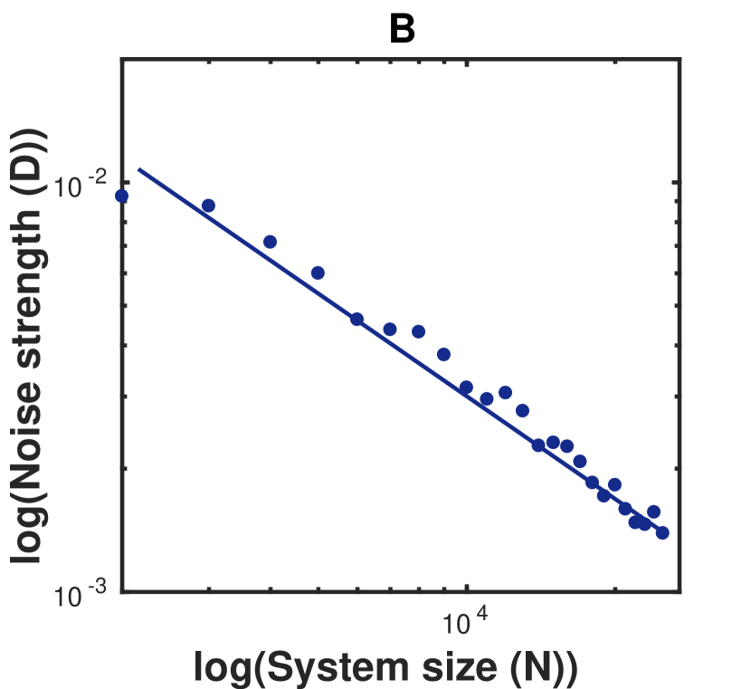
Given the demographic nature of the noise, we expect fluctuations to become less and less important with increasing $N$. Figure 5 shows that, as expected, $D$ has a reversed relationship with the system size $N$.

Figure 5: Quantifying the noise strength along the limit cycle. (A) Phase variance over time for different values of system size. (B) the noise strength versus $N$. Parameters in these figures are $\tau=0.5$, $a=1$ and $\sigma=3.05$ and the variance is calculated over 500 realizations of the system.

III.3 Analytic Approximation for the Noise Strength

In order to study the perturbations during evolution of the system around the limit cycle, we write the Fokker-Planck equation [17] of the stochastic RMA model by expanding the master equation for large values of $N$. We obtain the following equation:

$$\begin{split}\partial_{t}P(x,y)=&-\dfrac{\partial}{\partial x}F_{x}P(x,y)-\dfrac{\partial}{\partial y}F_{y}P(x,y)\\ &+\dfrac{1}{2N}\dfrac{\partial^{2}}{\partial x^{2}}B_{xx}P(x,y)+\dfrac{1}{2N}\dfrac{\partial^{2}}{\partial y^{2}}B_{yy}P(x,y)\\ &+\dfrac{1}{2N}\dfrac{\partial^{2}}{\partial x\partial y}B_{xy}P(x,y)+\dfrac{1}{2N}\dfrac{\partial^{2}}{\partial y\partial x}B_{yx}P(x,y),\end{split}$$ (10)

where $P(x,y)$, is the probability to find the system with abundances $(x,y)=(R/N,F/N)$ at time $t$ and:

$$F_{x}=ax-\dfrac{x^{2}}{2}-\dfrac{\sigma xy}{1+\sigma\tau x},$$

$$F_{y}=\dfrac{\sigma xy}{1+\sigma\tau x}-y,$$

$$B_{xx}=\dfrac{1}{N}(ax+\dfrac{x^{2}}{2}+\dfrac{\sigma xy}{1+\sigma\tau x}),$$

$$B_{yy}=\dfrac{1}{N}(\dfrac{\sigma xy}{1+\sigma\tau x}+y),$$

$$B_{xy}=B_{yx}=-\dfrac{1}{N}(\dfrac{\sigma xy}{1+\sigma\tau x}).$$ (11)

In the limit of weak noise, the Fokker-Planck equation can be expanded around the deterministic solution, scaled by the square root of the noise amplitude ($\mathbf{v}=\dfrac{1}{\sqrt{N}}(\mathbf{x}-\mathbf{x_{det}})$). This is called Van Kampen expansion [18, 17]. In this way, by omitting terms of higher order in $(1/N)^{-1/2}$, the Fokker-Planck equation can be transformed to the following equation:

$$\begin{split}\partial_{t}P(\mathbf{v},t)=&-\sum_{i,j}A_{ij}(t)\dfrac{\partial}{\partial v_{i}}v_{i}P(\mathbf{v},t)\\ &+\dfrac{1}{2}\sum_{i,j}\tilde{B}_{ij}\dfrac{\partial^{2}}{\partial v_{i}\partial v_{j}}P(\mathbf{v},t),\end{split}$$ (12)

where

$$A_{ij}=\dfrac{\partial F_{i}}{\partial v_{j}}|_{\mathbf{x_{det}(t)}},$$

$$\tilde{B}_{ij}=B_{ij}|_{\mathbf{x_{det}(t)}}.$$ (13)

Since we approximated the shape of the limit cycle with an ellipse, we can write the deterministic solution in the following form:

$$\mathbf{x_{det}}=\mathbf{x}_{f}+\begin{bmatrix}r(t)\cos\theta(t)\\ \epsilon r(t)\sin\theta(t)\ \end{bmatrix}.$$ (14)

To investigate the stochastic RMA system, we decompose the noise term into the normal $\xi_{n}$ and tangent $\xi_{l}$ direction along the limit cycle, corresponding respectively to amplitude and phase fluctuations. The two components $\xi_{n}$ and $\xi_{l}$ can be obtained using:

$$\mathbf{x}=\mathbf{x_{det}}+(r^{*}(t)+\dfrac{\xi_{n}}{\sqrt{N}})\begin{bmatrix}\cos(\omega t+\dfrac{\xi_{l}}{\sqrt{N}})\\ \epsilon\sin(\omega t+\dfrac{\xi_{l}}{\sqrt{N}})\ \end{bmatrix},$$ (15)

in this equations $r^{*}=\left\langle r\right\rangle$ and $\omega=\epsilon$ according to the eq. 8. By expanding the noise terms for large $N$ we find that:

$$\mathbf{x_{det}}=\mathbf{x_{f}}+\begin{bmatrix}r^{*}(t)\cos(\omega t)\\ \epsilon r^{*}(t)\sin(\omega t)\end{bmatrix}+(\dfrac{1}{\sqrt{N}})\begin{bmatrix}\xi_{x}\\ \xi_{y}\end{bmatrix},$$ (16)

where:

$$\xi_{x}=\xi_{n}\cos(\omega t)-\xi_{l}r^{*}(t)\sin(\omega t),$$

$$\xi_{y}=\xi_{n}\epsilon\sin(\omega t)-\xi_{l}\epsilon r^{*}(t)\cos(\omega t).$$ (17)

The Langevin equation corresponding to the $\xi_{x}$ and $\xi_{y}$ are written as:

$$\dot{\xi_{x}}=\sum_{i}A_{x,i}+\eta_{x},$$

$$\dot{\xi_{y}}=\sum_{i}A_{y,i}+\eta_{y},$$ (18)

where $\eta$ is related to the noise terms of Fokker-Planck equations as following:

$$\left\langle\eta_{x}^{2}\right\rangle=B_{xx},$$

$$\left\langle\eta_{y}^{2}\right\rangle=B_{yy},$$

$$\left\langle\eta_{x}\eta_{y}\right\rangle=B_{xy}.$$ (19)

The value of $\left\langle\dot{\xi_{l}^{2}}\right\rangle$ can be found by straight forward calculations from equations 17 and 18as follows:

$$\left\langle\dot{\xi_{l}^{2}}\right\rangle=\left\langle\dot{\xi_{l}^{2}}\right\rangle_{det}+Dt,$$ (20)

$$D=\dfrac{1}{2r^{2}\epsilon^{2}N}\left[\epsilon^{2}(ax+\dfrac{x^{2}}{2}+\dfrac{xy\sigma}{1+x\tau\sigma})+y+\dfrac{xy\sigma}{1+x\tau\sigma}\right].$$

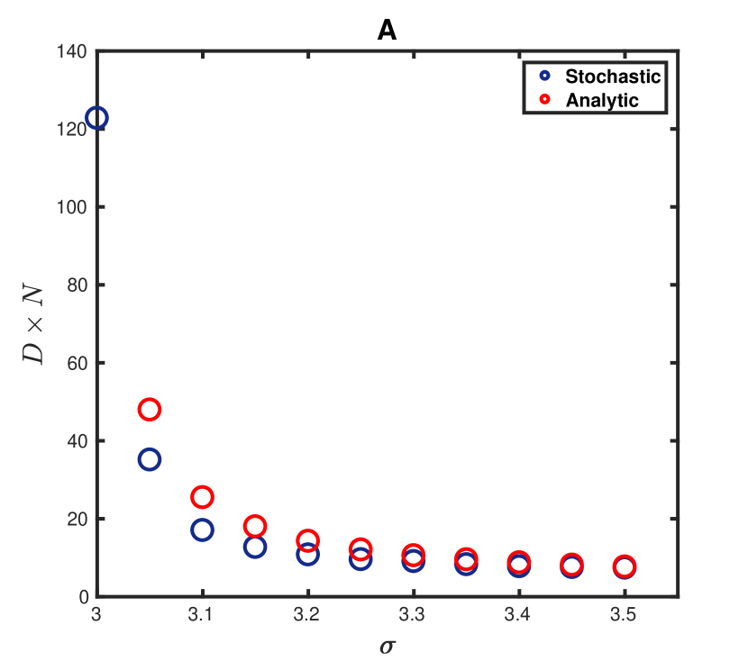
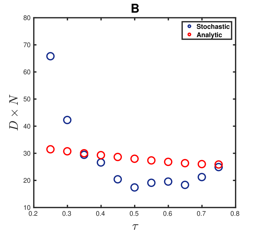
Where the averaging is over different realizations and one period of time. Figure 5 shows the noise strength versus $N$. The dependency of noise strength on $N$ obtained from stochastic simulations is in agreement with the analytical ones. Figure 6 shows the dependency of the effective diffusion constant $D$ on the parameters $\sigma$ and $\tau$. When $\sigma$ is close to the $\sigma^{*}$ (i.e., $\gamma\to 0$) the results of analytical approximation and simulation match well.

Figure 6: Comparison of the stochastic and analytical noise strength for different parameters. Parameters are $\gamma=0.03$, $a=1$, $\tau=0.5$ and $N=25000$.

IV Discussion

Oscillatory behavior in the populations has been widely reported in natural ecosystems and laboratory-scale experiments. Mathematical modeling of the interaction between predator and prey populations leads to the nonlinear ordinary differential equations that the time-dependent solutions of them are associated with limit cycle oscillations. Demographic stochasticity, due to unpredictability of the timing of birth, death, and interaction events, is often neglected and can remarkably alter the dynamics of a system.

In this paper, we have quantified the strength of the perturbations, due to the demographic effects of interacting species, in the limit cycle of the Roseznweig-MacArthur model. We showed that, in the vicinity of the bifurcation point we can approximate the limit cycle with an ellipse. In this limit, we obtained analytically the mean frequency and mean radius of the limit cycle as functions of the RMA parameters.

We then focus on the effect of stochasticity on the fluctuations along the limit cycle, that we effectively model as an angular Brownian motion. By expanding the master equation of the population densities through the Van Kampen system size method, we found demographic noise strength analytically, which has an inverse relationship with the system size. Finally, we compared our analytical results with the results found using simulation of the stochastic Rosenzweig-MacArthur model by Gillespie algorithm. A close agreement is observed between analytical results and the results found from the simulations.

Our work shows how the effect of demographic stochasticity on the frequency and phase of oscillation can be analytically captured even for non-linear model, at least in some parameter regime.