Multiconfigurational time-dependent density functional theory for atomic nuclei: Technical and numerical aspects

Abstract

The nuclear time-dependent density functional theory (TDDFT) is a tool of choice for describing various dynamical phenomena in atomic nuclei. In a recent study, we reported an extension of the framework - the multiconfigurational TDDFT (MC-TDDFT) model - that takes into account quantum fluctuations in the collective space by mixing several TDDFT trajectories. In this article, we focus on technical and numerical aspects of the model. We outline the properties of the time-dependent variational principle that is employed to obtain the equation of motion for the mixing function. Furthermore, we discuss evaluation of various ingredients of the equation of motion, including the Hamiltonian kernel, norm kernel, and kernels with explicit time derivatives. We detail the numerical methods for resolving the equation of motion and outline the major assumptions underpinning the model. A technical discussion is supplemented with numerical examples that consider collective quadrupole vibrations in ⁴⁰Ca, particularly focusing on the issues of convergence, treatment of linearly dependent bases, energy conservation, and prescriptions for the density-dependent part of an interaction.

1 Introduction

The nuclear time-dependent density functional theory (TDDFT) simenel2010 ; lacroix2004 ; simenel2012 ; bulgac2013 ; nakatsukasa2016 ; stevenson2019 ; schunck2019 is a tool of choice for describing the dynamical phenomena in atomic nuclei such as collective vibrations, low-energy heavy-ion reactions, or fission. Similarly to TDDFT approaches used in various branches of physics and chemistry casida12 ; marques2012 , it models the dynamics of a complex many-body system in terms of a product-type wave function whose diabatic time evolution is determined by a set of Schrödinger-like equations for the corresponding single-(quasi)particle states. While such an approach includes the one-body dissipation mechanism and is well-suited for calculating mean values of observables, it yields quasi-classical equations of motion in the collective space blaizot1986 ; ring2004 . Consequently, it drastically underestimates fluctuations of observables and is unable to account for quantum many-body effects such as tunneling in collective potential energy landscapes. The numerous attempts to include quantum fluctuations beyond the basic TDDFT framework can be broadly classified into two categories. On the one hand, the deterministic approaches include methods based on the truncation of the Bogolyubov-Born-Green-Kirkwood-Yvon (BBGKY) hierarchy bogolyubov1946 ; born1946 ; kirkwood1946 , leading to various time-dependent $n$-particle reduced density matrix (TD-nRDM) models bonitz2016 ; lackner2015 ; lackner2017 , the statistical treatment of complex internal degrees of freedom, leading to the Fokker-Planck framework dietrich2010 , and the Balian-Vénéroni variational principle balian1984 ; balian1992 ; simenel2011 . On the other hand, the stochastic approaches aim to replace a complex initial problem with a set of simpler problems, as seen in the stochastic mean-field theory reinhard1992 ; reinhard1992b ; lacroix2006 ; ayik2008 ; lacroix2014 or the exact quantum jump technique juillet2002 ; lacroix2005 . However, most of these methods face challenges when applied in conjunction with TDDFT due to the lack of a clear prescription for treating effects beyond the independent particle approximation. The stochastic mean-field theory, combined with TDDFT, has been applied with some success in describing fluctuations in fission tanimura2017 . Nevertheless, as demonstrated in Refs. regnier2018 ; regnier2019 , a proper description of quantum effects in the collective space requires a genuine quantization that accounts for the interference between different trajectories. Despite this, a fully quantum multiconfigurational extension, which is nowadays routinely employed in static calculations bender2003 ; egido2016 ; robledo2019 ; niksic2011 , has until very recently not been implemented in the TDDFT case.

Today, the multiconfigurational models of nuclear dynamics are largely restricted to the adiabatic time-dependent generator coordinate method (TDGCM) berger1984 ; goutte2004 ; younes2019 ; verriere2020 , typically supplemented with the Gaussian overlap approximation (GOA) brink1968 ; naoki1975 . Despite their significant success in describing numerous aspects of fission regnier2016 ; schunck2016 ; bender2020 , the existing TDGCM implementations consider only static states on the adiabatic collective potential energy landscapes and do not account for dissipation of the collective motion into disordered internal single-particle motion. Recently, the TDGCM framework was extended with a statistical dissipative term in the case of fission zhao2022a ; zhao2022b , while an earlier attempt to explicitly include two-quasiparticle excitations bernard2011 is yet to be implemented in a computationally feasible framework. However, the adiabatic approximation still imparts significant practical and formal difficulties to all these models schunck2016 , including the need to consider an extremely large number of static configurations, discontinuous potential energy surfaces, and the ill-defined scission line for fission. Consequently, a fully quantum framework is called for that would leverage the dissipative and fluctuation aspects of nuclear dynamics by removing the adiabatic assumption and mixing time-dependent configurations.

Theoretical foundations of such a framework were laid out already in the 1980s by Reinhard, Cusson, and Goeke reinhard1983 ; reinhard1987 . However, the rather limited computational capabilities of the time prevented any practical implementations beyond simplified models applied to schematic problems. A step towards more realistic applications was recently made in regnier2019 , where a multiconfigurational model was used to study the pair transfer between two simple superfluid systems interacting with a pairing Hamiltonian. Soon after, a collision between two $\alpha$-particles was studied within a fully variational model based on the Gaussian single-particle wave functions and a schematic Hamiltonian interaction hasegawa2020 . While it was argued that the model described quantum tunneling, a discussion ensued on whether the observed phenomenon can indeed be considered tunneling ono2022 ; hasegawa2022comment ; ono2022reply . Recently, we reported the first calculations in atomic nuclei where TDDFT configurations were mixed based on the energy density functionals (EDFs) framework marevic2023 . In there, we have shown that the collective multiphonon states emerge at high excitation energies when quantum fluctuations in the collective space are included beyond the independent particle approximation. A similar model, based on relativistic EDFs, was employed in a study of nuclear multipole vibrations li2023 and subsequently extended with pairing correlations to make it applicable to the fission phenomenon li2023b .

The ongoing developments and the increase of computational capabilities should, in the near future, render these models applicable to a wide range of nuclear phenomena. The goal of this manuscript is to provide more details on technical and numerical aspects of the multi-configurational time-dependent density functional theory (MC-TDDFT) framework reported in marevic2023 . In Sec. 2, we outline properties of the MC-TDDFT state and show how the time-dependent variational principle leads to the equation of motion for the mixing function. In Sec. 3, we discuss evaluation of various ingredients of the equation of motion, including the Hamiltonian kernel, the norm kernel, and kernels with explicit time derivatives. Sec. 4 contains details on resolving the equation of motion and calculating various observables, as well as a discussion on the overall algorithmic complexity of the framework. The technical discussion is supplemented with numerical examples in Sec. 5. Finally, Sec. 6 brings summary of the present work.

2 The MC-TDDFT state and its time evolution

2.1 Preliminaries

Motivated by the well-known static generator coordinate method (GCM) hill1953 ; griffin1957 , the dynamic MC-TDDFT state can be written as

$$\ket{\Psi(t)}=\int\!\,d\mathbf{q}~{}f_{\bm{q}}(t)\ket{\Phi_{\bm{q}}(t)},$$ (1)

where $\bm{q}$ denotes a set of continuous generating coordinates, $\ket{\Phi_{\bm{q}}(t)}$ are the time-dependent, many-body generating states, and $f_{\bm{q}}(t)$ is the mixing function which is to be determined through a variational principle (see Sec. 2.2 and 2.3). Depending on the application, there exists a large freedom in choosing various ingredients of Eq. (1):

• The generating coordinates represent collective degrees of freedom associated to modes whose quantum fluctuations are being considered. In static DFT, they are often related to the magnitude or the phase of a complex order parameter corresponding to one or several broken symmetries sheikh2019 . Within adiabatic TDGCM studies of nuclear fission, one typically considers multipole moments regnier2016 ; schunck2016 , pairing strength sadhukhan2014pairinginduced ; zhao2016multidimensionallyconstrained ; bernard2019role and occasionally also the nuclear temperature zhao2022a ; zhao2022b . In recent dynamical MC-TDDFT studies, a gauge angle was considered as a generating coordinate in the case of pair transfer between superfluid systems regnier2019 , the relative position and momentum for collisions hasegawa2020 , and multipole boost magnitudes or multipolarities for vibrations marevic2023 ; li2023 .

• The generating states are typically chosen as Slater determinants hasegawa2020 ; marevic2023 ; li2023 or the $U(1)$-symmetry-breaking quasiparticle vacua regnier2019 . The corresponding single-particle wave functions may be built upon a simple ansatz, such as Gaussians hasegawa2020 , or can be obtained from microscopic calculations, based on schematic interactions regnier2019 or actual EDFs marevic2023 ; li2023 ; li2023b . In the limiting case where the generating states are time-independent and are obtained through energy minimization under constraints, we recover the conventional adiabatic TDGCM framework. Irrespective of the nature of generating states, an optimal choice of the basis set will take into account minimization of overlaps within the set, with the goal of reducing linear dependencies and ensuring that each state carries a sufficient distinct physical information. Any remaining linear dependencies are later explicitly removed, as described in Sec. 3.3 and 5.3.

• In principle, one could apply the variational principle with respect to both the mixing function $f_{\bm{q}}(t)$ and the generating states $\ket{\Phi_{\bm{q}}(t)}$. Such a strategy generally yields a rather complicated set of coupled time-dependent differential equations. It is employed, for example, in quantum chemistry within the multi-configurational time-dependent Hartree-Fock (MC-TDHF) framework meyer2009multidimensional . Note, however, that this framework encompasses only the special case of Hamiltonian theories with orthogonal generating states. Applications in nuclear physics, where the generating states are typically non-orthogonal, have so far remained restricted to the toy-model calculation of Ref. hasegawa2020 . A simplification that has been adopted in recent applications regnier2019 ; marevic2023 ; li2023 is to treat variationally only the mixing function, while assuming that the generating states follow independent trajectories. In Ref. reinhard1983 it was shown that the lowest order of GOA yields independent trajectories even when the generating states are treated variationally.

2.2 Equation of motion for the mixing function

The backbone idea of the MC-TDDFT framework is to look for an approximate solution of the time-dependent Schrödinger equation that takes the form of Eq. (1) and is parametrized by the complex mixing function $f_{\bm{q}}(t)$. Different variants of the time-dependent variational principle can be used to obtain the dynamical equation for the mixing function yuan2019theory . In this work, we consider the following action:

$$\begin{split}S(f,f^{*},\xi_{1})&=\int_{t_{0}}^{t_{1}}\,dt\braket{\Psi(t)}{\hat{H}-i\hbar\partial_{t}}{\Psi(t)}\\ &+\int_{t_{0}}^{t_{1}}\,dt\,\xi_{1}(t)\Big{(}\braket{\Psi(t)}{\Psi(t)}-1\Big{)}.\\ \end{split}$$ (2)

Here, the first term integrates the Lagrangian of the system over time and the second term imposes normalization of the solution by introducing a real Lagrange multiplier $\xi_{1}(t)$. We look for a mixing function $f(t)$ that makes this action stationary,

$$\delta S=0,$$ (3)

where the variation is taken with respect to any complex function $f(t)$ and any value of the Lagrange multiplier $\xi_{1}(t)$, while keeping their values fixed at the endpoints, $\delta f(t_{0})=\delta f(t_{1})=\delta\xi_{1}(t_{0})=\delta\xi_{1}(t_{1})=0$. This equation is formally equivalent to the system of equations

$$\frac{\partial S}{\partial f}=0,\quad\frac{\partial S}{\partial f^{*}}=0,\quad\frac{\partial S}{\partial\xi_{1}}=0.$$ (4)

Writing explicitly the derivatives of the action yields a set of integro-differential equations for the mixing function,

$$i\hbar\dot{f}^{\dagger}\mathcal{N}(t) =f^{\dagger}(t)\Big{[}-\mathcal{H}(t)+\mathcal{D}(t)-i\hbar\dot{\mathcal{N}}(t)$$

$$\qquad-\xi_{1}(t)\mathcal{N}(t)\Big{]},$$ (5a)

$$i\hbar\mathcal{N}(t)\dot{f}(t) =\Big{[}\mathcal{H}(t)-\mathcal{D}(t)+\xi_{1}(t)\mathcal{N}(t)\Big{]}f(t),$$ (5b)

$$f^{\dagger}(t)\mathcal{N}(t)f(t) =1.$$ (5c)

We use here a compact matrix notation with respect to the collective coordinate $\bm{q}$. The norm (overlap) kernel reads

$$\mathcal{N}_{\bm{q}\bm{q^{\prime}}}(t)=\braket{\Phi_{\bm{q}}(t)}{\Phi_{\bm{q^{\prime}}}(t)}.$$ (6)

Equations (5) and (5b) also involve the Hamiltonian kernel

$$\mathcal{H}_{\bm{q}\bm{q^{\prime}}}(t)=\braket{\Phi_{\bm{q}}(t)}{\hat{H}}{\Phi_{\bm{q^{\prime}}}(t)},$$ (7)

and the time derivative kernel defined as

$$\mathcal{D}_{\bm{q}\bm{q^{\prime}}}(t)=\braket{\Phi_{\bm{q}}(t)}{i\hbar\partial_{t}}{\Phi_{\bm{q^{\prime}}}(t)}.$$ (8)

The identity

$$i\hbar\dot{\mathcal{N}}(t)=\mathcal{D}(t)-\mathcal{D}^{\dagger}(t)$$ (9)

implies that Eq. (5) is just the conjugate transpose of Eq. (5b). Finally, one can insert these equations into the time derivative of Eq. (5c) to show that any value of the Lagrange parameter $\xi_{1}(t)$ gives a proper solution of the system of equations as long as the initial state is normalized. In fact, the $\xi_{1}(t)$ term in the equation of motion only multiplies the function $f(t)$ by a time-dependent phase during the dynamics. Setting this Lagrange parameter to zero yields the compact equation of motion

$$i\hbar\dot{f}(t) =\mathcal{N}^{-1}(t)\Big{[}\mathcal{H}(t)-\mathcal{D}(t)\Big{]}f(t).$$ (10)

This equation differs from the adiabatic TDGCM equation to the extent that (i) all the kernels are time-dependent and (ii) there is an additional term involving the time derivative kernel $\mathcal{D}(t)$.

2.3 Dealing with time-dependent, non-orthogonal generating states

In the present case, a particular caution is necessary because we employ a family of generating states $|\Phi_{\bm{q}}(t)\rangle$ which is generally linearly dependent. Consequently, the mapping between the mixing functions $f_{\bm{q}}(t)$ and the many-body state $\ket{\Psi(t)}$ is not bijective ring2004 . More specifically, at each time $t$, one may diagonalize the norm kernel

$$\mathcal{N}_{\bm{q}\bm{q^{\prime}}}(t)=\sum_{k}\mathcal{U}_{\bm{q}k}(t)\lambda_{k}(t)\mathcal{U}_{\bm{q^{\prime}}k}^{\dagger}(t).$$ (11)

The columns of $\mathcal{U}(t)$ form an orthonormal eigenbasis of the space of mixing functions $\mathcal{F}$ so that we can always expand them as

$$f_{\bm{q}}(t)=\sum_{k}f_{k}(t)\mathcal{U}_{\bm{q}k}(t).$$ (12)

Furthermore, the norm eigenvalues $\lambda_{k}(t)$ can be used to split the full space $\mathcal{F}$ into the direct sum

$$\mathcal{F}=\mathcal{I}(t)\oplus\mathcal{K}(t).$$ (13)

Here, $\mathcal{I}(t)$ is the image of $\mathcal{N}(t)$, sometimes also referred to as the range of $\mathcal{N}(t)$ saad2003iterative . It corresponds to the vector space of functions spanned by the columns of $\mathcal{U}(t)$ associated to $\lambda_{k}(t)>0$. Equivalently, the kernel vector space $\mathcal{K}(t)$ is spanned by the columns of $\mathcal{U}(t)$ with $\lambda_{k}(t)=0$. In the following, we sort by convention the eigenvalues of $\mathcal{N}(t)$ in the ascending order so that the first $d\!-\!r$ eigenvalues will be zero, where $d$ and $r$ are the dimension and the rank of $\mathcal{N}(t)$, respectively. We can then introduce the projectors $\mathcal{P}^{\mathcal{I}}(t)$ and $\mathcal{P}^{\mathcal{K}}(t)$ on the subspaces $\mathcal{I}(t)$ and $\mathcal{K}(t)$, respectively, with the corresponding matrices

$$\mathcal{P}^{\mathcal{I}}_{\bm{q}\bm{q^{\prime}}}(t)=\sum_{k>d-r}\mathcal{U}_{\bm{q}k}(t)\mathcal{U}_{\bm{q^{\prime}}k}^{\dagger}(t),$$ (14)

$$\mathcal{P}^{\mathcal{K}}_{\bm{q}\bm{q^{\prime}}}(t)=\sum_{k\leq d-r}\mathcal{U}_{\bm{q}k}(t)\mathcal{U}_{\bm{q^{\prime}}k}^{\dagger}(t).$$ (15)

The sum of the two projectors satisfies

$$\mathcal{P}^{\mathcal{I}}(t)+\mathcal{P}^{\mathcal{K}}(t)=\mathbb{1}_{\mathcal{F}}.$$ (16)

Moreover, per definition, the norm matrix is entirely contained in the image subspace and the same applies to the kernel of any observable $\hat{O}$,

$$\mathcal{P}^{\mathcal{K}}(t)\mathcal{N}(t) =0,$$ (17a)

$$\mathcal{P}^{\mathcal{I}}(t)\mathcal{N}(t) =\mathcal{N}(t),$$ (17b)

$$\mathcal{P}^{\mathcal{I}}(t)\mathcal{O}(t) =\mathcal{O}(t),$$ (17c)

where $\mathcal{O}_{\bm{q}\bm{q^{\prime}}}(t)=\braket{\Phi_{\bm{q}}(t)}{\hat{O}}{\Phi_{\bm{q^{\prime}}}(t)}$.

With these definitions at hand, we can now make explicit a property of the MC-TDDFT ansatz which is well known already from the static GCM framework ring2004 : at any time, the component of the mixing function $f(t)$ belonging to the kernel space $\mathcal{K}(t)$ does not contribute to the many-body state $|\psi(f(t))\rangle$. In other words,

$$|\psi[f(t)]\rangle=|\psi\left[\mathcal{P}^{I}(t)f(t)\right]\rangle.$$ (18)

Going one step further, one can show that the ansatz (1) provides a one-to-one mapping between the complex mixing functions living in the space $\mathcal{I}(t)$ and the MC-TDDFT many-body states. Although this property brings no formal difficulties, it has to be taken into account when numerically simulating the time evolution of a system. Indeed, the naive equation of motion (10) could easily lead to the accumulation of large or even diverging components of $f(t)$ in $\mathcal{K}(t)$, or to fast time oscillations of $f(t)$ in this subspace. This type of unphysical behavior may prevent a reliable computation of the mixing function in practice.

To circumvent this problem, it is possible to look for a solution of the time-dependent variational principle that has a vanishing component in $\mathcal{K}(t)$ for all $t$,

$$\mathcal{P}^{\mathcal{K}}(t)f(t)=0.$$ (19)

Such a solution is obtained by minimizing the augmented action

$$\begin{split}\tilde{S}(f,f^{*},\xi_{1},\xi_{2})&=S(f,f^{*},\xi_{1})\\ &+\int_{t_{0}}^{t_{1}}\,dt\,\xi_{2}(t)||\mathcal{P}^{\mathcal{K}}f||^{2}.\end{split}$$ (20)

Compared to Eq. (2), this relation introduces a new term with the Lagrange parameter $\xi_{2}(t)$ that ensures the constraint (19). The same reasoning as in Sec. 2.2 leads to the modified equation of motion

$$i\hbar\dot{f}(t)=\mathcal{N}^{-1}(t)\Big{[}\mathcal{H}(t)-\mathcal{D}(t)\Big{]}f(t)+i\hbar\dot{\mathcal{P}}^{\mathcal{I}}(t)f(t).$$ (21)

The last term on the right hand side ensures that the mixing function stays in the subspace $\mathcal{I}(t)$ at all time. In the same way as for $\xi_{1}(t)$ in (4), any value of $\xi_{2}(t)$ leads to a proper solution of the variational principle as long as $f$ is solution of (21). We therefore set it to zero. Solving Eq. (21) instead of Eq. (10) provides a better numerical stability at the price of estimating $\dot{\mathcal{P}}^{\mathcal{I}}(t)$ at each time step.

2.4 Equation of motion for the collective wave function

In principle, the mixing function could be determined by numerically integrating Eq. (21). However, like in the static GCM, it is useful to introduce the collective wave function $g(t)$ as

$$g(t)=\mathcal{N}^{1/2}(t)f(t).$$ (22)

The square root of the norm kernel is defined by the relation

$$\mathcal{N}_{\bm{q}\bm{q^{\prime}}}(t)=\int_{\bm{q^{\prime\prime}}}\,d\bm{q^{\prime\prime}}\mathcal{N}_{\bm{q}\bm{q^{\prime\prime}}}^{1/2}(t)\mathcal{N}_{\bm{q^{\prime\prime}}\bm{q^{\prime}}}^{1/2}(t).$$ (23)

At any time, the collective wave function $g(t)$ belongs to the subspace $\mathcal{I}(t)$ and uniquely defines the MC-TDDFT state. Following a standard procedure, we also transform kernels $\mathcal{O}(t)$ to their collective operators $\mathcal{O}^{c}(t)$,

$$\mathcal{O}^{c}(t)=\mathcal{N}^{-1/2}(t)\mathcal{O}(t)\mathcal{N}^{-1/2}(t).$$ (24)

This provides a useful mapping

$$\langle\hat{O}\rangle(t)=g^{\dagger}(t)\mathcal{O}^{c}(t)g(t)$$ (25)

for any observable $\hat{O}$. Inserting the definition of the collective wave function into Eq. (10) or (21) yields the equivalent equation of motion for the collective wave function,

$$i\hbar\dot{g}(t)=\Big{(}\mathcal{H}^{c}(t)-\mathcal{D}^{c}(t)+i\hbar\dot{\mathcal{N}}^{1/2}(t)\mathcal{N}^{-1/2}(t)\Big{)}g(t).$$ (26)

For numerical purposes, the total kernel on the right hand side of Eq. (26) can be recast in an explicitly Hermitian form,

$$i\hbar\dot{g}(t)=\Big{[}\mathcal{H}^{c}(t)+\mathcal{T}_{1}^{c}(t)+\mathcal{T}_{2}^{c}(t)\Big{]}g(t),$$ (27)

with two Hermitian kernels

$$\mathcal{T}_{1}^{c}(t) =-\frac{1}{2}\big{(}\mathcal{D}^{c}(t)+\mathcal{D}^{c\dagger}(t)\big{)},$$ (28a)

$$\mathcal{T}_{2}^{c}(t) =\frac{i\hbar}{2}\big{(}\dot{\mathcal{N}}^{1/2}(t)\mathcal{N}^{-1/2}(t)-\mathcal{N}^{-1/2}(t)\dot{\mathcal{N}}^{1/2}(t)\big{)}.$$ (28b)

The equation of motion (27) is the one that is numerically solved in the numerical examples of Sec. 5 and in our previous work marevic2023 .

2.5 Definition of the generating states

In this work, the generating states are built as Slater determinants of independent single-particle states

$$\ket{\Phi_{\bm{q}}(t)}=\prod_{k=1}^{A}a_{k}^{\bm{q}\dagger}(t)\ket{0},$$ (29)

where $A$ is the number of particles, $\ket{0}$ is the particle vacuum, and $\{a_{k}^{\bm{q}\dagger}(t),a_{k}^{\bm{q}}(t)\}$ is a set creation and annihilation operators associated to the single-particle states. The single-particle states can be expanded in the spatial representation,

$$a_{k}^{\bm{q}\dagger}(t)= \sum_{\sigma}\int_{\bm{r}}d^{3}\bm{r}\varphi_{k}^{\bm{q}}(\bm{r}\sigma;t)c_{\bm{r}\sigma}^{\dagger},$$ (30)

$$a_{k}^{\bm{q}}(t)= \sum_{\sigma}\int_{\bm{r}}d^{3}\bm{r}\varphi_{k}^{\bm{q}*}(\bm{r}\sigma;t)c_{\bm{r}\sigma},$$ (31)

where $c^{\dagger}_{\bm{r}\sigma}$ (resp. $c_{\bm{r}\sigma}$) creates (resp. annihilates) a nucleon of spin $\sigma$ at position $\bm{r}$. The $k$-th single-particle wave function $\varphi_{k}^{\bm{q}}$ of the generating state labeled by $\bm{q}$ reads

$$\varphi_{k}^{\bm{q}}(\bm{r}\sigma;t)=\langle\bm{r}\sigma|a^{\bm{q}\dagger}_{k}(t)|0\rangle.$$ (32)

The single-particle wave functions (32) for neutrons or protons can be decomposed as

$$\begin{split}\varphi_{k}^{\bm{q}}(\bm{r}\sigma;t)&=\Big{(}\varphi_{k,0}^{\bm{q}}(\bm{r};t)+i\varphi_{k,1}^{\bm{q}}(\bm{r};t)\Big{)}\chi_{\uparrow}(\sigma)\\ &+\Big{(}\varphi_{k,2}^{\bm{q}}(\bm{r};t)+i\varphi_{k,3}^{\bm{q}}(\bm{r};t)\Big{)}\chi_{\downarrow}(\sigma).\end{split}$$ (33)

The four real spatial functions $\varphi_{k,\alpha}^{\bm{q}}(\bm{r};t)$ with $\alpha=0,3$ correspond, respectively, to the real spin-up, imaginary spin-up, real spin-down, and imaginary spin-down component, and $\chi_{\uparrow/\downarrow}(\sigma)$ are the eigenstates of the $z$ component of the spin operator.

Starting from some initial conditions, the generating states $\ket{\Phi_{\bm{q}}(t)}$ are then assumed to evolve independently from each other, according to the nuclear TDHF equations simenel2010 ; lacroix2004 ; simenel2012 ,

$$i\hbar\dot{\rho}_{\bm{q}}(t)=\Big{[}h[\rho_{\bm{q}}(t)],\rho_{\bm{q}}(t)\Big{]},$$ (34)

where $\rho_{\bm{q}}(t)$ is the one-body density matrix corresponding to $\ket{\Phi_{\bm{q}}(t)}$ and $h[\rho_{\bm{q}}(t)]$ is the single-particle Hamiltonian derived from a Skyrme EDF bender2003 ; schunck2019 .

3 Calculation of kernels

3.1 The norm kernel

The overlap of two Slater determinants is given by the determinant of the matrix containing overlaps between the corresponding single-particle states lowdin1955 ; plasser2016 ,

$$\mathcal{N}_{\bm{q}\bm{q^{\prime}}}(t)=\det M_{\bm{q}\bm{q^{\prime}}}(t).$$ (35)

In the absence of isospin mixing, the total overlap corresponds to the product of overlaps for neutrons ($\tau=n$) and protons ($\tau=p$),

$$\mathcal{N}_{\bm{q}\bm{q^{\prime}}}(t)=\prod_{\tau=n,p}\mathcal{N}_{\bm{q}\bm{q^{\prime}}}^{(\tau)}(t)=\prod_{\tau=n,p}\det M_{\bm{q}\bm{q^{\prime}}}^{(\tau)}(t),$$ (36)

where the elements of $M_{\bm{q}\bm{q^{\prime}}}^{(\tau)}(t)$ read

$$\Big{[}M_{\bm{q}\bm{q^{\prime}}}^{(\tau)}(t)\Big{]}_{kl}=\braket{\varphi_{k}^{\bm{q}(\tau)}(t)}{\varphi_{l}^{\bm{q^{\prime}}(\tau)}(t)},$$ (37)

or explicitly

$$\Big{[}M_{\bm{q}\bm{q^{\prime}}}^{(\tau)}(t)\Big{]}_{kl}=\sum_{\sigma}\int\,d^{3}\bm{r}\varphi_{k}^{\bm{q}(\tau)*}(\bm{r}\sigma;t)\varphi_{l}^{\bm{q^{\prime}}(\tau)}(\bm{r}\sigma;t).{}$$ (38)

In addition to the norm kernel matrix $\mathcal{N}$(t), Eq. (27) requires evaluation of the square root of its inverse, $\mathcal{N}^{-1/2}(t)$. This matrix is straightforward to calculate when $\mathcal{N}(t)$ is non-singular. The case of a singular norm kernel matrix is discussed in Sec. 3.3.

3.2 The Hamiltonian kernel

3.2.1 General expressions

Motivated by the generalized Wick theorem balian1969 , the Hamiltonian kernel can be expressed as

$$\mathcal{H}_{\bm{q}\bm{q^{\prime}}}(t)=E_{\bm{q}\bm{q^{\prime}}}(t)\mathcal{N}_{\bm{q}\bm{q^{\prime}}}(t),$$ (39)

where the energy kernel $E_{\bm{q}\bm{q^{\prime}}}(t)$ is obtained as a spatial integral of the energy density kernel

$$E_{\bm{q}\bm{q^{\prime}}}(t)=\int\,d^{3}\bm{r}\mathcal{E}_{\bm{q}\bm{q^{\prime}}}(\bm{r};t).$$ (40)

The energy density kernel itself corresponds to the sum of kinetic, nuclear (Skyrme), and Coulomb components,

$$\mathcal{E}_{\bm{q}\bm{q^{\prime}}}(\bm{r};t)=\mathcal{E}_{\bm{q}\bm{q^{\prime}}}^{\rm{Kin}}(\bm{r};t)+\mathcal{E}_{\bm{q}\bm{q^{\prime}}}^{\rm{Sky}}(\bm{r};t)+\mathcal{E}_{\bm{q}\bm{q^{\prime}}}^{\rm{Cou}}(\bm{r};t),$$ (41)

and it is a functional of the one-body, non-local transition density

$$\rho_{\bm{q}\bm{q^{\prime}}}(\bm{r}\sigma,\bm{r^{\prime}}\sigma^{\prime};t)=\frac{\braket{\Phi_{\bm{q}}(t)}{c^{\dagger}_{\bm{r^{\prime}}\sigma^{\prime}}c_{\bm{r}\sigma}}{\Phi_{\bm{q^{\prime}}}(t)}}{\braket{\Phi_{\bm{q}}(t)}{\Phi_{\bm{q^{\prime}}}(t)}}.$$ (42)

This density is used to derive various local transition density components that will appear in (41). The explicit expressions for all the components are given in A.

3.2.2 Energy density components

To start with, the kinetic energy density can be simply calculated as

$$\mathcal{E}_{\bm{q}\bm{q^{\prime}}}^{\rm{Kin}}(\bm{r};t)=\frac{\hbar^{2}}{2m}\sum_{\tau=n,p}\tau^{(\tau)}_{\bm{q}\bm{q^{\prime}}}(\bm{r};t),$$ (43)

where $m$ is the nucleon mass and $\tau_{\bm{q}\bm{q^{\prime}}}^{(\tau)}(\bm{r};t)$ is the local transition kinetic density [Eq. (79)].

Furthermore, the nuclear potential component of the energy density is derived from the Skyrme pseudopotential schunck2019 . The proton-neutron representation of the energy density is equivalent to the one used in Ref. bonche1987 , except that the diagonal local densities are substituted by transition local densities defined in A. The full expression reads

$$\begin{split}\mathcal{E}_{\bm{q}\bm{q^{\prime}}}^{\rm{Sky}}(\bm{r};t)&=B_{1}\rho_{\bm{q}\bm{q^{\prime}}}^{2}(\bm{r};t)+B_{2}\sum_{\tau=n,p}\rho_{\bm{q}\bm{q^{\prime}}}^{(\tau)2}(\bm{r};t)\\ &+B_{3}\big{(}\rho_{\bm{q}\bm{q^{\prime}}}(\bm{r};t)\tau_{\bm{q}\bm{q^{\prime}}}(\bm{r};t)-\bm{j}_{\bm{q}\bm{q^{\prime}}}^{2}(\bm{r};t)\big{)}\\ &+B_{4}\sum_{\tau=n,p}\big{(}\rho_{\bm{q}\bm{q^{\prime}}}^{(\tau)}(\bm{r};t)\tau_{\bm{q}\bm{q^{\prime}}}^{(\tau)}(\bm{r};t)-\bm{j}_{\bm{q}\bm{q^{\prime}}}^{(\tau)2}(\bm{r};t)\big{)}\\ &+B_{5}\rho_{\bm{q}\bm{q^{\prime}}}(\bm{r};t)\Delta\rho_{\bm{q}\bm{q^{\prime}}}(\bm{r};t)\\ &+B_{6}\sum_{\tau=n,p}\rho_{\bm{q}\bm{q^{\prime}}}^{(\tau)}(\bm{r};t)\Delta\rho_{\bm{q}\bm{q^{\prime}}}^{(\tau)}(\bm{r};t)\\ &+B_{7}\rho_{D}^{\alpha}(\bm{r};t)\rho_{\bm{q}\bm{q^{\prime}}}^{2}(\bm{r};t)\\ &+B_{8}\rho_{D}^{\alpha}(\bm{r};t)\sum_{\tau=n,p}\rho_{\bm{q}\bm{q^{\prime}}}^{(\tau)2}(\bm{r};t)\\ &+B_{9}\rho_{\bm{q}\bm{q^{\prime}}}(\bm{r};t)\big{(}\nabla\cdot{\rm{\bm{J}}}_{\bm{q}\bm{q^{\prime}}}(\bm{r};t)\big{)}\\ &+B_{9}\bm{j}_{\bm{q}\bm{q^{\prime}}}(\bm{r};t)\cdot\big{(}\nabla\times\bm{s}_{\bm{q}\bm{q^{\prime}}}(\bm{r};t)\big{)}\\ &+B_{9}\sum_{\tau=n,p}\rho_{\bm{q}\bm{q^{\prime}}}^{(\tau)}(\bm{r};t)\big{(}\nabla\cdot{\rm{\bm{J}}}_{\bm{q}\bm{q^{\prime}}}^{(\tau)}(\bm{r};t)\big{)}\\ &+B_{9}\bm{j}_{\bm{q}\bm{q^{\prime}}}^{(\tau)}(\bm{r};t)\cdot\big{(}\nabla\times\bm{s}_{\bm{q}\bm{q^{\prime}}}^{(\tau)}(\bm{r};t)\big{)}\\ &+B_{10}\bm{s}_{\bm{q}\bm{q^{\prime}}}^{2}(\bm{r};t)+B_{11}\sum_{\tau=n,p}\bm{s}_{\bm{q}\bm{q^{\prime}}}^{(\tau)2}(\bm{r};t)\\ &+B_{12}\rho_{D}^{\alpha}(\bm{r};t)\bm{s}_{\bm{q}\bm{q^{\prime}}}^{2}(\bm{r};t)\\ &+B_{13}\rho_{D}^{\alpha}(\bm{r};t)\sum_{\tau=n,p}\bm{s}_{\bm{q}\bm{q^{\prime}}}^{(\tau)2}(\bm{r};t).{}\end{split}$$ (44)

The coupling constants $B_{i}$ and parameter $\alpha$ are defined in B. The $\rho_{D}(\bm{r};t)$ density is defined in Sec. 3.2.3.

Finally, the Coulomb component is composed of the direct and the exchange contribution,

$$\mathcal{E}_{\bm{q}\bm{q^{\prime}}}^{\rm{Cou}}(\bm{r};t)=\mathcal{E}_{\bm{q}\bm{q^{\prime}}}^{\rm{Cou,Dir}}(\bm{r};t)+\mathcal{E}_{\bm{q}\bm{q^{\prime}}}^{\rm{Cou,Exc}}(\bm{r};t).$$ (45)

The direct contribution is calculated as

$$\mathcal{E}_{\bm{q}\bm{q^{\prime}}}^{\rm{Cou,Dir}}(\bm{r};t)=\frac{1}{2}~{}U_{\bm{q}\bm{q^{\prime}}}^{\rm{Cou,Dir}}(\bm{r};t)\rho_{\bm{q}\bm{q^{\prime}}}^{(p)}(\bm{r};t),$$ (46)

where $\rho_{\bm{q}\bm{q^{\prime}}}^{(p)}(\bm{r};t)$ is the local proton density [Eq. (77)] and $U_{\bm{q}\bm{q^{\prime}}}^{\rm{Cou,Dir}}(\bm{r};t)$ is the Coulomb potential obtained as the solution of the Poisson equation

$$\Delta U_{\bm{q}\bm{q^{\prime}}}^{\rm{Cou,Dir}}(\bm{r};t)=-4\pi\frac{e^{2}}{4\pi\epsilon_{0}}\rho_{\bm{q}\bm{q^{\prime}}}^{(p)}(\bm{r};t).$$ (47)

The real and the imaginary component of the potential are obtained by solving the corresponding differential equations separately, subject to the Dirichlet condition at the boundary $\bm{r}_{B}$,

$$U_{\bm{q}\bm{q^{\prime}}}^{\rm{Cou,Dir}}(\bm{r}_{B};t)=\frac{e^{2}}{4\pi\epsilon_{0}}\frac{Z_{\bm{q}\bm{q^{\prime}}}(t)}{|\bm{r}_{B}|}.$$ (48)

Here, $Z_{\bm{q}\bm{q^{\prime}}}(t)$ is a complex number,

$$Z_{\bm{q}\bm{q^{\prime}}}(t)=\int\,d^{3}\bm{r}\rho_{\bm{q}\bm{q^{\prime}}}^{(p)}(\bm{r};t),$$ (49)

naturally giving a boundary condition for both the real and the imaginary component of the potential. Note that the condition (48) is based on the multipole expansion of a generalized charge truncated at zeroth order. Eventually, higher orders could be included as well. Finally, the exchage contribution is calculated at the Slater approximation

$$\mathcal{E}_{\bm{q}\bm{q^{\prime}}}^{\rm{Cou,Exc}}(\bm{r};t)=-\frac{3}{4}\frac{e^{2}}{4\pi\epsilon_{0}}\Big{(}\frac{3}{\pi}\Big{)}^{1/3}\Big{[}\rho_{D}^{(p)}(\bm{r};t)\Big{]}^{4/3},$$ (50)

where $\rho_{D}^{(p)}(\bm{r};t)$ is the local proton density calculated according to a prescription, as described in Sec. 3.2.3.

3.2.3 Density-dependent prescription

The local transition density is generally a complex quantity and its non-integer powers are not uniquely defined. Consequently, a prescription is needed to evaluate $\rho_{D}^{\alpha}(\bm{r})$ in (44) and (50). This is a well-known feature of multi-reference EDF models which has been thoroughly discussed in the literature robledo2010 ; sheikh2019 . In the present implementation, we opt for the average density prescription,

$$\rho_{D}^{\alpha}(\bm{r};t)=\Big{[}\frac{1}{2}\Big{(}\rho_{\bm{q}\bm{q}}(\bm{r};t)+\rho_{\bm{q^{\prime}}\bm{q^{\prime}}}(\bm{r};t)\Big{)}\Big{]}^{\alpha},$$ (51)

which is always real and reduces to the diagonal local density when $\bm{q}=\bm{q^{\prime}}$. An alternative form of the average density prescription duguet2003 ,

$$\rho_{D}^{\alpha}(\bm{r};t)=\frac{1}{2}\Big{(}\rho_{\bm{q}\bm{q}}^{\alpha}(\bm{r};t)+\rho_{\bm{q^{\prime}}\bm{q^{\prime}}}^{\alpha}(\bm{r};t)\Big{)},$$ (52)

satisfies the same properties but is obviously not equivalent to (51). Other choices, such as the mixed density prescription and the projected density prescription, have also been considered in the literature, primarily in the context of symmetry restoration robledo2010 ; sheikh2019 . Sensitivity of calculations to the choice of prescription is discussed in Sec. 5.5.

3.3 Inverse of the norm kernel

Solving Eq. (27) requires inverting the norm kernel matrix $\mathcal{N}$(t). The matrix $\mathcal{N}^{-1/2}(t)$ is then plugged into the last term of (27), and is also used to evaluate the collective kernels $\mathcal{H}^{c}(t)$ and $\mathcal{D}^{c}(t)$, according to (24). Formally, the square root inverse $\mathcal{N}^{-1/2}(t)$ is soundly defined in the image subspace $\mathcal{I}(t)$ only. Consequently, this linear operator always acts on functions belonging to the image subspace, both in the equation of motion [Eq. (27)] and in the definition of collective kernels [Eq. (24)]. We compute its matrix elements in the $\bm{q}$ representation as

$${\mathcal{N}}^{-1/2}_{\bm{q}\bm{q^{\prime}}}(t)=\sum_{k>d-r}\mathcal{U}_{\bm{q}k}(t)\lambda_{k}^{-1/2}(t)\mathcal{U}^{\dagger}_{\bm{q^{\prime}}k}(t),$$ (53)

where the sum runs only over strictly positive eigenvalues $\lambda_{k}$.

In practical applications, diagonalizing the norm kernel typically yields several eigenvalues that are numerically close to zero but not exactly vanishing. It is well known from static GCM bender2003 ; robledo2019 and TDGCM verriere2020 that taking into account the inverse of these eigenvalues and the associated eigenstates in the sum (53) gives rise to numerical instabilities. A standard procedure consists of introducing a cutoff parameter $\lambda_{\rm{cut}}$ and considering all norm eigenvalues $\lambda_{k}<\lambda_{\rm{cut}}$ as numerical zeros. In all the following applications, the square root of the inverse norm kernel is therefore approximated as the sum (53) running only over the eigenvalues $\lambda_{k}>\lambda_{\rm{cut}}$. The particular value of $\lambda_{\rm{cut}}$ depends on the application and should be carefully checked on a case-by-case basis (see Sec. 5.3). Too large cutoff values may lead to significant errors in estimation of the inverse, while too low values magnify numerical instabilities. Note that the described approach is equivalent to solving the problem in the collective space spanned by the so-called natural states,

$$\ket{k(t)}=\sum_{\bm{q}}\frac{U_{\bm{q}k}(t)}{\sqrt{\lambda_{k}(t)}}\ket{\Phi_{\bm{q}}(t)},$$ (54)

with $\dim_{k}\leq\dim_{\bm{q}}$, and $\dim_{\bm{q}}$ is the dimension of the $\bm{q}-$basis space.

3.4 Kernels with explicit time derivatives

To ensure hermiticity of the total collective kernel on the right hand side of Eq. (27), it is crucial to use a consistent numerical prescription when evaluating its various ingredients. This particularly applies to kernels that include an explicit differentiation with respect to time, such as the $\mathcal{D}_{\bm{q}\bm{q^{\prime}}}(t)$, $\dot{\mathcal{N}}_{\bm{q}\bm{q^{\prime}}}(t)$, and $\dot{\mathcal{N}}^{1/2}_{\bm{q}\bm{q^{\prime}}}(t)$ kernel.

3.4.1 The $\mathcal{D}_{\bm{q}\bm{q^{\prime}}}(t)$ kernel

We assume that the time derivative of a generating state $\ket{\Phi_{\bm{q}}(t)}$ is well represented by finite differences,

$$\partial_{t}\ket{\Phi_{\bm{q}}(t)}\approx\frac{1}{\Delta t}\big{(}\ket{\Phi_{\bm{q}}(t)}-\ket{\Phi_{\bm{q}}(t_{-})}\big{)},$$ (55)

where $t_{-}=t-\Delta t$ and $\Delta t$ is the time step. The time-derivative kernel (8) can then be simply evaluated as

$$\mathcal{D}_{\bm{q}\bm{q^{\prime}}}(t)=\frac{i\hbar}{\Delta t}\big{(}\braket{\Phi_{\bm{q}}(t)}{\Phi_{\bm{q^{\prime}}}(t)}-\braket{\Phi_{\bm{q}}(t)}{\Phi_{\bm{q^{\prime}}}(t_{-})}\big{)}.$$ (56)

Calculation of the time-derivative kernel was therefore reduced to evaluation of two overlap kernels equivalent to those in Eq. (6).

3.4.2 The $\dot{\mathcal{N}}_{\bm{q}\bm{q^{\prime}}}(t)$ and $\dot{\mathcal{N}}^{1/2}_{\bm{q}\bm{q^{\prime}}}(t)$ kernels

We start by evaluating the $\dot{\mathcal{N}}_{\bm{q}\bm{q^{\prime}}}(t)$ kernel,

$$\dot{\mathcal{N}}_{\bm{q}\bm{q^{\prime}}}(t)=\braket{\Phi_{\bm{q}}(t)}{\dot{\Phi}_{\bm{q^{\prime}}}(t)}+\braket{\dot{\Phi}_{\bm{q}}(t)}{\Phi_{\bm{q^{\prime}}}(t)}.$$ (57)

Using the finite differences scheme of (55), we obtain

$$\begin{split}\dot{\mathcal{N}}_{\bm{q}\bm{q^{\prime}}}(t)=\frac{1}{\Delta t}\big{(}&2\braket{\Phi_{\bm{q}}(t)}{\Phi_{\bm{q^{\prime}}}(t)}-\braket{\Phi_{\bm{q}}(t)}{\Phi_{\bm{q^{\prime}}}(t_{-})}\\ -&\braket{\Phi_{\bm{q}}(t_{-})}{\Phi_{\bm{q^{\prime}}}(t)}\big{)}.\end{split}$$ (58)

Similarly as before, we only need to evaluate three overlap kernels. In the next step, we can determine the $\dot{\mathcal{N}}^{1/2}(t)$ kernel by recognizing that

$$\dot{\mathcal{N}}(t)=\dot{\mathcal{N}}^{1/2}(t)\mathcal{N}^{1/2}(t)+\mathcal{N}^{1/2}(t)\dot{\mathcal{N}}^{1/2}(t)$$ (59)

represents a special case of the Sylvester equation bhatia1997 . If $\mathcal{N}^{1/2}(t)$ has all positive, non-zero eigenvalues, there exists a unique solution which can be written as

$${\rm vec}\big{(}\dot{\mathcal{N}}^{1/2}(t)\big{)}=\mathcal{S}^{-1}(t)~{}{\rm vec}\big{(}\dot{\mathcal{N}}(t)\big{)},$$ (60)

where the vectorization operator ”$\rm{vec}$” corresponds to stacking the columns of a $d\times d$ matrix into a vector of length $d^{2}$ and

$$\mathcal{S}(t)=\mathbb{1}\otimes\mathcal{N}^{1/2}(t)+\big{(}\mathcal{N}^{1/2}(t)\big{)}^{T}\otimes\mathbb{1}$$ (61)

is a complex matrix belonging to $\mathbb{C}^{d^{2}\times d^{2}}$. We recover the desired kernel in its matrix form with the inverse of the vectorization operator.

$$\dot{\mathcal{N}}^{1/2}(t)={\rm vec}^{-1}\big{[}\mathcal{S}^{-1}(t)~{}{\rm vec}\big{(}{\dot{\mathcal{N}}(t)}\big{)}\big{]}.$$ (62)

Note that the described procedure requires inverting the $\mathcal{S}(t)$ matrix, whose dimension grows as a square of the number of basis states. However, for the basis sizes envisioned in applications of MC-TDDFT (from several states to several tens of states), such inversions are feasible. Should the need for even larger bases occur, hermiticity of the norm matrix may be used to further reduce the dimensionality of the problem (for example, by using the half-vectorization instead of the vectorization operation). Finally, this procedure to solve the Sylvester equation involves inversion of the matrix $\mathcal{S}(t)$ which can be positive semi-definite, similarly to $\mathcal{N}^{-1/2}$. Following the same procedure, we diagonalize the matrix that should be inverted, keep only the non-zero eigenvalues, and invert the matrix in this subspace. This yields the $\mathcal{S}(t)$ matrix which can be safely used in Eq. (62).

4 Resolution of the equation of motion and calculation of observables

Once all the expressions for collective kernels have been established as described in Sec. 3, the MC-TDDFT calculations proceed in three major steps: (i) choosing a set of initial conditions relevant for the physical case under study, (ii) integrating in time the equation of motion for the basis states [Eq. (34)] and the collective wave function [Eq. (27)], and (iii) computing observables of interest.

4.1 The initial conditions

To start with, the initial mixing functions $f_{\bm{q}}(0)$ need to be chosen. This choice is somewhat arbitrary as it is entirely guided by the physical scenario one aims to simulate. For example, in marevic2023 we mixed three TDDFT states ($\bm{q}=1,2,3$) and considered two sets of initial conditions. In the first case, we set $f_{1}(0)=1,f_{2}(0)=f_{3}(0)=0$, rendering the initial MC-TDDFT state equal to the first TDDFT state. In the second case, the mixing functions were determined by diagonalizing the initial collective Hamiltonian kernel, thus starting calculations from the actual multiconfigurational ground state. Of course, alternative choices are also possible.

Furthermore, the initial total collective kernel on the right hand side of (27) needs to be determined. While the $\mathcal{H}^{c}(t)$ and $\mathcal{N}^{-1/2}(t)$ are uniquely defined at $t=0$, this is not the case for the $\mathcal{D}^{c}(t)$ and $\dot{\mathcal{N}}^{1/2}(t)$ that include explicit time derivatives and are calculated with the finite difference scheme. The value of these kernels at $t=0$ is therefore estimated by propagating the set of basis states by $\Delta t$ and using the finite differences scheme. Since for sufficiently small time steps the collective kernels evolve very smoothly, the overall dynamics is not significantly impacted by this choice.

4.2 Numerical schemes for time propagation

The nuclear TDHF equation [Eq. (34)] can be efficiently resolved by using any of the popular numerical schemes. In the present implementation, we use the fourth order Runge-Kutta method (RK4) which was in regnier2019 shown to provide better norm conservation properties than the Crank-Nicolson scheme. On the other hand, the equation of motion for collective wave functions [Eq. (27)] is resolved by the direct method, that is

$$g_{\bm{q}}(t_{0}+\Delta t)=\exp\Big{(}-\frac{i}{\hbar}\mathcal{T}(t_{0})\Delta t\Big{)}g_{\bm{q}}(t_{0}),$$ (63)

where $\mathcal{T}(t)$ is the total collective kernel on the right hand side of (27). The direct method appears feasible for smaller sets of basis states. For larger sets, an alternative method such as the RK4 may be better suited.

4.3 Calculation of observables

Following Eq. (25), the collective wave function can be used to calculate the expectation value of any observable in the MC-TDDFT state at any time $t$. Generally, the collective kernel $\mathcal{O}^{c}(t)$ can be calculated from the usual kernel according to (24). In the specific case of a one-body, spin-independent, local observable, the generalized Wick theorem yields directly

$$\begin{split}\mathcal{O}_{\bm{q}\bm{q^{\prime}}}(t)&=\mathcal{N}_{\bm{q}\bm{q^{\prime}}}(t)\int\,d^{3}\bm{r}O(\bm{r})\rho_{\bm{q}\bm{q^{\prime}}}(\bm{r};t),\end{split}$$ (64)

where $\rho_{\bm{q}\bm{q^{\prime}}}(\bm{r};t)$ is the transition particle density from Eq. (77) and $O(\bm{r})$ is the coordinate space representation of the corresponding operator. For example, for the multipole moment operator $O_{lm}(\bm{r})=r^{l}Y_{lm}(\theta,\phi)$, where $Y_{lm}(\theta,\phi)$ are the spherical harmonics. Furthermore, the variance of such one-body observable in a normalized MC-TDDFT state can be calculated as

$$\sigma^{2}_{\hat{O}}(t)=\braket{\Psi(t)}{\hat{O}^{2}}{\Psi(t)}-\braket{\Psi(t)}{\hat{O}}{\Psi(t)}^{2}.$$ (65)

An explicit expression of the variance as a function of the one-body density is given in C.

4.4 Overall algorithmic complexity

In this section, we provide an estimate of how the MC-TDDFT framework scales with various parameters of the problem. The parameters driving the complexity of the MC-TDDFT equation [Eq. (27)] are the size of the spatial basis $b$ ($=2\times m_{x}$, where $m_{x}$ is the number of mesh points and $2$ is the spin factor), the number of particles $A$, the number of generating states $d$, and the number of time iterations $n_{t}$. For each time iteration, one needs to compute all the kernels, propagate all the generating states, and finally propagate the collective wave function.

Following the discussion of Sec. 3, we can estimate the computational complexity of different kernels:

• Norm (overlap) kernel: $O(d^{2}\times A^{2}\times b)+O(d^{2}\times A^{3})$. The first term comes from the determination of all pairs of $M_{\bm{q}\bm{q^{\prime}}}$ matrices, while the second term results from the computation of their determinants. Since our application relies on a spatial representation for which $b\gg A$, the second term is negligible.

• Derivative kernel: $O(d^{2}\times A^{2}\times b)$. This kernel is evaluated by calculating two overlap kernels and therefore exhibits the same computational complexity.

• Hamiltonian kernel (given the overlap kernel): $O(d^{2}\times A^{2}\times b)$. Calculation of this kernel requires inversion of all $M_{\bm{q}\bm{q^{\prime}}}$ matrices at the cost of $O(d^{2}\times A^{3})$, computation of all transition densities at the cost of $O(d^{2}\times A^{2}\times b)$, and finally the spatial integration of all terms in the energy density kernel at the cost of $O(d^{2}\times b)$. Note that the zero range of the Skyrme effective interaction avoids the presence of terms proportional to $b^{2}$ that would significantly increase the computational burden. Assuming again $b\gg A$ renders the term associated with $d^{2}\times A^{2}\times b$ the dominant term. In practice, we observe that computing the Hamiltonian kernel is the most costly operation (and by far more costly than the computation of the overlap kernel, even though they scale equally).

• Time derivative of $\mathcal{N}^{1/2}$: $O(d^{6})$. This high cost as a function of the number of generating states comes from the inversion of the matrix in Eq. (61).

Similar considerations yield a complexity of $O(d\times A\times b)$ for the time propagation of the generating states and a complexity of $O(d^{2})$ for the time propagation of the collective wave function. Keeping only the leading contributions, we conclude that the overall complexity of MC-TDDFT calculations using the present method scales as $O(n_{t}\times d^{2}\times A^{2}\times b)+O(n_{t}\times d^{6})$. The leading contributions to this cost come from the calculation of kernels and, more specifically, the calculation of transition densities (first term) and the inversion of the Sylvester matrix (second term).

For comparison, a standard TDGCM model with $d^{\prime}$ static generating states has a computational complexity of $O(d^{\prime 2}\times A^{2}\times b)+O(n_{t}\times d^{\prime 2})$. The first term corresponds to a single computation of all the time-independent kernels, while the second term corresponds to the time propagation of the collective wave function. Under the assumption that the two models can describe a certain nuclear reaction with similar accuracy, this analysis shows that MC-TDDFT outperforms TDGCM when a small number of trajectories is sufficient. In particular, neglecting the $O(n_{t}\times d^{6})$ term, we estimate that MC-TDDFT becomes computationally cheaper when

$$d<\frac{d^{\prime}}{\sqrt{n_{t}}}.$$ (66)

In practice, the variational spaces spanned by the two methods are different and the philosophy of MC-TDDFT as compared to the standard TDGCM is to rely on a fewer number of generating states that already encompass the time-odd physics. Of course, the two methods may not be equally well-adapted to describe different phenomena and a more quantitative comparison dedicated to a few nuclear processes would be welcome in the near future.

5 Illustrative calculations

As an illustrative example, we consider the doubly-magic nucleus ⁴⁰Ca. Like in Ref. marevic2023 , the calculations are performed using a newly developed code based on the finite element method zienkiewicz2013 ; mfem . The nuclear dynamics is simulated in a three-dimensional box of length $L$, with a regular mesh of $N$ cells in each spatial direction and a finite element basis of $n$-th order polynomials. We employ the SLy4d EDF kim1997 , whose parameters were adjusted without the center of mass correction, making it particularly well suited for dynamical studies. Unless stated otherwise, the average density prescription of the form (51) is used for the density-dependent part of an effective interaction.

In Sec. 5.1, we briefly demonstrate the convergence of TDDFT calculations with the new code. In Sec. 5.2, we discuss the convergence of collective dynamics when two TDDFT trajectories are mixed. In Sec. 5.3, we discuss the treatment of linear dependencies in the TDDFT basis, using an example of mixing of three trajectories. Furthermore, in Sec. 5.4 we address the issue of energy conservation within the MC-TDDFT framework. Finally, the influence of the density prescription on results is discussed in Sec. 5.5.

5.1 Convergence of TDDFT calculations

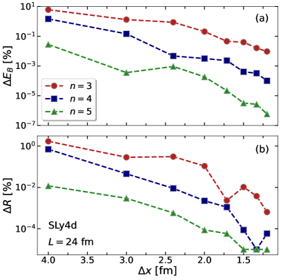
Figure 1: Convergence $\Delta X=|(X-X_{0})/X_{0}|\cdot 100$ of the ground-state binding energy ($X\equiv E_{B}$, panel (a)) and the ground-state root mean square radius ($X\equiv R=\sqrt{\langle r^{2}\rangle}$, panel (b)) as a function of the mesh step size $\Delta x=L/N$, where $L=24$ fm is the box length and $N$ is the number of finite element cells per spatial dimension. Convergence patterns are compared for finite element bases of polynomials of the order $n=3,4,5$. The fully converged values $E_{0}=-339.118594$ MeV and $R_{0}=3.413466$ fm were obtained with $(n=5,\Delta x=24/26$ fm $\approx 0.92$ fm). These values agree within at least $1$ keV and $0.003$ fm, respectively, with those obtained using the HFBTHO computational framework marevic2022 . Note that the radius is fully converged for $(n=5,\Delta x\leq 1.5$ fm); the corresponding values are plotted as $10^{-5}$.

In Fig. 1(a), we demonstrate the convergence of the calculated ground-state binding energy $E_{B}$ by plotting $\Delta E_{B}=|(E_{B}-E_{0})/E_{0}|\cdot 100$ as a function of the mesh step size $\Delta x=L/N$, where $E_{0}$ is the fully converged value (up to the sixth decimal point). An equivalent quantity for the ground-state root mean square radius, $\Delta R$, is shown in Fig. 1(b). The box length is fixed to $L=24$ fm in all calculations and polynomials of the order $n=3,4,5$ are considered for the finite element basis. As expected, the bases of higher order polynomials systematically require smaller numbers of cells (larger $\Delta x$) to obtain a comparable convergence. For example, the binding energy in the ($n=3$, $\Delta x_{1}=24/14$ fm $\approx 1.71$ fm) calculation converges within $0.05\%$, while already the ($n=5,\Delta x_{2}=2.4$ fm) calculation converges within $0.001\%$. The equivalent holds for radii, even though they converge at a somewhat faster rate.

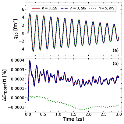
Figure 2: (a): Isoscalar quadrupole moment of the $q_{20}$-boosted TDDFT state for different spatial and temporal discretization schemes: $(n=3,\Delta x_{1},\Delta t_{1})$ in red, $(n=3,\Delta x_{1},\Delta t_{2})$ in blue, and $(n=5,\Delta x_{2},\Delta t_{2})$ in green, with $\Delta x_{1}\approx 1.71$ fm, $\Delta x_{2}=2.4$ fm, $\Delta t_{1}=5\cdot 10^{-4}$ zs, and $\Delta t_{2}=10^{-4}$ zs. (b): Numerical error of the TDDFT energy, $\Delta E_{\rm{TDDFT}}(t)=\Big{(}E(t)-E(0)\Big{)}/E(0)\cdot 100$, for the three cases above.

In the next step, the ⁴⁰Ca ground state is given an instantaneous isoscalar quadrupole boost by applying the corresponding operator simenel2012 ; scamps2013 , $\exp(i\eta\hat{Q}_{20})$, where $\eta=5.7\cdot 10^{-3}$ fm^-2 is the boost magnitude and $\hat{Q}_{20}=r^{2}Y_{20}(\theta)=(1/4)\sqrt{5/\pi}(2z^{2}-x^{2}-y^{2})$ is the axially-symmetric quadrupole moment operator. To verify convergence of the resulting TDDFT dynamics, in Fig. 2(a) we compare time evolutions of the quadrupole moment, $q_{20}(t)=\braket{\Phi_{\bm{q}}(t)}{\hat{Q}_{20}}{\Phi_{\bm{q}}(t)}$, for $(n=3,\Delta x_{1})$ and $(n=5,\Delta x_{2})$ space discretizations. The time propagation is performed using the fourth order Runge-Kutta method and is traced up to $t=3$ zs.

The $(n=3,\Delta x_{1})$ dynamics is well converged for a wide range of time steps $\Delta t$; as can be seen in Fig. 2(a), the quadrupole moments $q_{20}(t)$ obtained with $\Delta t_{1}=5\cdot 10^{-4}$ zs and $\Delta t_{2}=10^{-4}$ zs are essentially indistinguishable. A similar holds for the $(n=5,\Delta x_{2})$ case, even though achieving convergence with higher order basis functions and/or finer spatial meshes will generally necessitate using smaller time steps $\Delta t$. For example, the $(n=5,\Delta x_{2})$ calculations do not converge for $\Delta t_{1}$. However, the $q_{20}(t)$ obtained with $\Delta t_{2}$ is indistinguishable from the two curves obtained with $(n=3,\Delta x_{1})$. This indicates that the minor difference in ground-state convergence of the two sets of spatial parameters bears no significant consequence for the subsequent TDDFT dynamics.

This is further corroborated by Fig. 2(b), showing the variation of the TDDFT energy $E(t)$ as a function of time, $\Delta E_{\rm{TDDFT}}(t)=\Big{(}E(t)-E(0)\Big{)}/E(0)\cdot 100$. The energy should be exactly conserved within the TDDFT framework - therefore, the small variations observed in Fig. 2(b) stem from numerical effects. Standard causes for such variations include the discretization errors in the estimation of the spatial derivatives, leading to a non-Hermitian mean-field Hamiltonian, as well as approximations of the time propagator acting on the single-particle wave functions that break unitarity schuetrumpf2018tdhf ; jin2021lise . Even though calculations with $(n=5,\Delta x_{2})$ yield comparatively smaller variations, these remain rather low in the $(n=3,\Delta x_{1})$ case; under $0.0004\%$ or less than $1$ keV. In addition, note that variations are independent of the time step.

5.2 Convergence of the collective dynamics

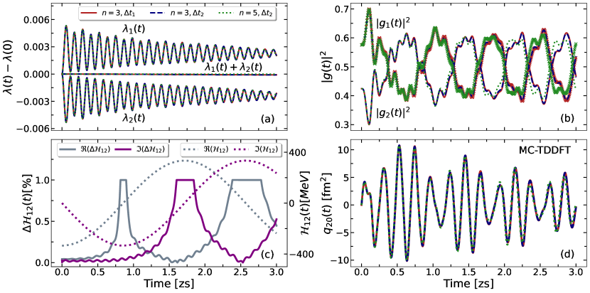
Figure 3: Mixing of two TDDFT configurations, discussed in Sec.  5.2, for three sets of spatial and temporal parameters, described in caption to Fig. 2. (a): Time evolution of the norm kernel matrix eigenvalues with respect to their initial values. The two eigenvalues oscillate in counterphase, such that their sum always remains constant. (b): Squared modulus of the collective wave function. Note that the $|g_{1}(t)|^{2}$ component is distinguished from the $|g_{2}(t)|^{2}$ component by the crossed markers while keeping the same color convention. Their sum remains equal to one at all times, reflecting the unitarity of collective dynamics. (c): The difference, in percentage, between the off-diagonal component of the Hamiltonian kernel calculated with the two sets of spatial parameters, $\Delta\mathcal{H}_{12}(t)=\Big{|}\Big{(}\mathcal{H}_{12}^{n=3}(t)-\mathcal{H}_{12}^{n=5}(t)\Big{)}/\mathcal{H}_{12}^{n=5}(t)\Big{|}\cdot 100$, where $\mathcal{H}_{12}^{n=3}(t)$ is calculated with $(n=3,\Delta x_{1})$ and $\mathcal{H}_{12}^{n=5}(t)$ with $(n=5,\Delta x_{2})$. The right $y$-axis shows the time evolution of $\mathcal{H}_{12}^{n=5}(t)$. In both cases, the real and the imaginary component are plotted separately. The difference $\Delta\mathcal{H}_{12}(t)$ diverges when $\mathcal{H}_{12}^{n=5}(t)$ changes sign - consequently, all points with $\Delta\mathcal{H}_{12}(t)>1\%$ are plotted as $1\%$. (d): The isoscalar quadrupole moment of the MC-TDDFT state obtained with the three sets of parameters.

As a first example of configuration mixing, we consider a mixed state composed of two TDDFT configurations,

$$\ket{\Psi_{A}(t)}=f_{1}(t)\ket{\Phi_{1}(t)}+f_{2}(t)\ket{\Phi_{2}(t)}.$$ (67)

Here, for $\ket{\Phi_{1}(t)}$ we take the TDDFT state described in the previous section, corresponding to the ⁴⁰Ca ground state which is given an isoscalar quadrupole boost of magnitude $\eta_{1}=5.7\cdot 10^{-3}$ fm^-2. Equivalently, $\ket{\Phi_{2}(t)}$ corresponds to the ground state boosted by $\eta_{2}=1.376\cdot 10^{-2}$ fm^-2. This choice of quadrupole boosts yields states with excitation energies of about $E_{1}(t=0)=0.25$ and $E_{2}(t=0)=1.46$ MeV above the Hartree-Fock ground state. At $t=0$, we set $f_{1}(0)=1$ and $f_{2}(0)=0$ so that the initial mixed state corresponds to the first basis state. The equation of motion for the collective wave function [Eq. (27)] is resolved by the direct method [Eq. (63)]. As before, the box length is fixed to $L=24$ fm. We consider the three sets of spatial and temporal parameters described in Sec. 5.1.

To start with, the initial eigenvalues of the norm kernel matrix read $\lambda_{1}(0)=0.011502$ and $\lambda_{2}(0)=1.988498$ for the $(n=3,\Delta x_{1})$ case, and $\lambda_{1}(0)=0.011491$ and $\lambda_{2}(0)=1.988509$ and for the $(n=5,\Delta x_{2})$ case. In Fig. 3(a), we show the time evolution of norm eigenvalues with respect to their initial values, $\lambda(t)-\lambda(0)$, for all three sets of parameters. The two eigenvalues oscillate in counterphase, such that their sum (the horizontal line in the middle of Fig. 3(a)) remains constant up to numerical accuracy. In this case, the dimension of the collective space is the same as the dimension of the basis space, $\dim_{k}=\dim_{\bm{q}}=2$. However, in many practical implementations the norm eigenstates corresponding to very small eigenvalues will need to be removed to ensure a stable numerical solution. This issue is addressed in Sec. 5.3.

In Fig. 3(b), we show the squared modulus of the collective wave function for the three parameter sets from Sec. 5.1. Once again, the $(n=3,\Delta x_{1})$ calculations are well-converged with respect to the time step $\Delta t$. Overall, the components of the collective wave function exhibit an oscillatory behavior. Their sum remains equal to one at all times, reflecting the unitarity of collective dynamics. Furthermore, the $(n=5,\Delta x_{2})$ curves are initially indistinguishable from the $n=3$ curves, but start to deviate for $t>1$ zs.

The source of these minor deviations can be traced back to different convergence profiles of the off-diagonal kernel elements in the equation of motion. As demonstrated earlier in Fig. 2, the diagonal components of the Hamiltonian kernel - that is, the TDDFT energies - show excellent convergence with respect to the choice of spatial discretization parameters. However, the off-diagonal components involve transition densities and are therefore expected to exhibit weaker convergence for the same choice of parameters. To shed more light on this issue, in Fig. 3(c) we show the difference, in percentage, between the off-diagonal component of the Hamiltonian kernel [Eq. (7)] calculated with the two sets of spatial parameters, $\Delta\mathcal{H}_{12}(t)=\Big{|}\Big{(}\mathcal{H}_{12}^{n=3}(t)-\mathcal{H}_{12}^{n=5}(t)\Big{)}/\mathcal{H}_{12}^{n=5}(t)\Big{|}\cdot 100$, where $\mathcal{H}_{12}^{n=3}(t)$ is calculated with $(n=3,\Delta x_{1})$ and $\mathcal{H}_{12}^{n=5}(t)$ with $(n=5,\Delta x_{2})$. Since $\mathcal{H}_{12}(t)$ is a complex quantity, the corresponding real and imaginary components are plotted separately. Furthermore, the right $y$-axis of Fig. 3(c) shows the real and the imaginary component of $\mathcal{H}^{n=5}_{12}(t)$. Please note that this quantity is not a constant; the question of energy conservation is addressed in more detail in Sec. 5.4.

Initially, both the real and the imaginary component of $\Delta\mathcal{H}_{12}(t)$ are relatively small. In addition, they stay well under $1\%$ for the largest part of time evolution. The sole exception are the regions around $t$ values where either the real or the imaginary component of $\mathcal{H}_{12}(t)$ changes sign (around $0.85$ zs and $2.6$ zs for the former and $1.7$ zs for the latter). In those cases, the denominator in $\Delta\mathcal{H}_{12}(t)$ becomes very small and the entire quantity tends to diverge. Consequently, for plotting purposes, all points with $\Delta\mathcal{H}_{12}(t)>1\%$ are shown as $1\%$. Nevertheless, note that the absolute value of deviation remains under $1$ MeV throughout the entire time evolution. While not drastic, such a deviation is sufficient to cause minor discrepancies seen in Fig. 3(b).

To examine the impact of this effect on an observable, in Fig. 3(d) we show time evolution of the isoscalar quadrupole moment of the MC-TDDFT state, $q_{20}(t)=\braket{\hat{Q}_{20}}(t)$ [Eq. (25) with $\hat{O}=\hat{Q}_{20}$]. The three sets of parameters again yield essentially indistinguishable results, except for some minor deviations of the $(n=5,\Delta x_{2})$ curve for larger values of $t$.

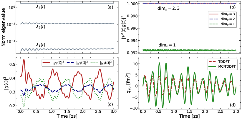
Figure 4: Mixing of three TDDFT configurations, discussed in Sec. 5.3, for $(n=3,\Delta x_{1})$ and $\Delta t_{1}=5\cdot 10^{-4}$ zs. (a): Time evolution of the norm kernel matrix eigenvalues. The three components oscillate in time, such that their sum remains constant. (b): Projection of the collective wave function onto the image subspace, $|\mathcal{P}^{\mathcal{I}}(t)g(t)|^{2}$, for three different choices of the norm eigenvalue cutoff (or, equivalently, three different dimensions of the collective space $\dim_{k}$). The $\dim_{k}=2$ provides numerical stability while ensuring $|\mathcal{P}^{\mathcal{I}}(t)g(t)|^{2}=1$ up to $\approx 10^{-7}$. (c): Squared modulus of the collective wave function for $\dim_{k}=2$. (d): The isoscalar quadrupole moment of a single TDDFT trajectory (red) and the MC-TDDFT state (green) for $\dim_{k}=2$.

Overall, a particular choice of spatial parameters will reflect a compromise between the feasibility of computational cost and the required accuracy. In the current case, the $(n=5,\Delta x_{2})$ parameters appear to yield somewhat more accurate results, but at the price of about three times longer computational time per iteration. Of course, this difference will become even larger as the basis size increases. Therefore, in the following, we will be using the $(n=3,\Delta x_{1})$ spatial parametrization - a choice which was also made in Ref. marevic2023 .

5.3 Treatment of linear dependencies in the basis

In the next example, we consider mixing of three TDDFT configurations,

$$\ket{\Psi_{B}(t)}=\sum_{i=1}^{3}f_{i}(t)\ket{\Phi_{i}(t)}.$$ (68)

Here, $\ket{\Phi_{1}(t)}$ and $\ket{\Phi_{3}(t)}$ correspond to the two configurations from the previous section. Furthermore, $\ket{\Phi_{2}(t)}$ is generated in the same manner, by applying the $q_{20}$-boost of the magnitude $\eta_{2}=1.14\cdot 10^{-2}$  fm^-2 to the ground state. This yields an excited state with $E_{2}(t=0)=1.00$ MeV. This choice of basis states is equivalent to the one made in Ref. marevic2023 . We also set $f_{1}(0)=1$ and $f_{2}(0)=f_{3}(0)=0$ so that the initial mixed state corresponds to the first basis state and coupling between the trajectories kicks in with time. We use $(n=3,\Delta x_{1})$, $\Delta t_{1}=5\cdot 10^{-4}$ zs, and set the box size to $L=24$ fm.

In Fig. 4(a), the time evolution of the eigenvalues of the corresponding norm matrix are shown. Starting from $\lambda_{1}(0)=8\cdot 10^{-6}$, $\lambda_{2}(0)=0.012162$, and $\lambda_{3}(0)=2.987830$, the three components oscillate in time, such that their sum remains constant (up to numerical accuracy). The amplitude of these oscillations is rather small, in agreement with the fact that each basis state itself describes a small-amplitude nuclear oscillation.

The collective wave function should, at all times, be contained in the image of $\mathcal{N}(t)$. In Fig. 4(b), we show the projection of the collective wave function onto the image subspace, $|\mathcal{P}^{\mathcal{I}}(t)g(t)|^{2}$, for three different choices of the collective space [Eq. (54)]. For $\dim_{k}=\dim_{\bm{q}}=3$, per definition, we have $|\mathcal{P}^{\mathcal{I}}(t)g(t)|^{2}=1$ for all $t$. However, the inclusion of a very small eigenvalue $\lambda_{1}(t)$ causes numerical instabilities. This leads to, for example, spurious small oscillations of the center of mass or to the total collective kernel on the right hand side of Eq. (26) not being exactly Hermitian. On the other hand, the $\dim_{k}=1$ choice yields $|\mathcal{P}^{\mathcal{I}}(t)g(t)|^{2}~{}\approx 0.992$, reflecting the fact that removing the relatively large norm eigenstate with $\lambda_{2}(t)\approx 0.01$ removes a portion of physical information as well. The collective space should correspond to the smallest subspace of the full Hilbert space containing all the basis states; for too large cutoffs, however, the collective space does not anymore contain all the basis states. Consequently, the $\dim_{k}=2$ choice is optimal in this case - while being numerically stable, it also ensures $|\mathcal{P}^{\mathcal{I}}(t)g(t)|^{2}=1$ up to $\approx 10^{-7}$. An equivalent analysis could be carried out looking at the Frobenius norm of $|\mathcal{P}^{I}(t)\mathcal{N}(t)-\mathcal{N}(t)|$ [Eq. (17b)] or to the partial sum of eigenvalues $\sum_{k\in\rm{Im}(\mathcal{N})}\lambda_{k}$.

In Fig. 4(c), we show the squared modulus of the resulting collective wave function, which again exhibits an oscillatory behavior. In particular, one can notice a close resemblance of $|g_{1}(t)|^{2}$ and $|g_{3}(t)|^{2}$ to the collective wave function from Fig. 3(b). This is entirely expected, since the corresponding collective spaces are both of dimension $2$ and spanned by very similar states.

Finally, Fig. 4(d) shows the isoscalar quadrupole moment of the $\ket{\Phi_{1}(t)}$ TDDFT trajectory and of the MC-TDDFT state. As already noted in Ref. marevic2023 , the TDDFT curve exhibits nearly harmonic oscillations of a single frequency, consistently with what is usually observed within TDDFT when the Landau damping effect is absent. The other two TDDFT trajectories (not shown) oscillate at the same frequency, but with slightly larger amplitudes. On the other hand, the MC-TDDFT curve is markedly more complex, exhibiting multiple frequencies, which can be related to the emergence of collective multiphonon excitations chomaz1995 ; aumann1998 in a requantized collective model. Consistently with remarks above, the MC-TDDFT curve closely resembles the corresponding curves from Fig. 3(d). Calculating the Fourier transform of the quadrupole response yields the multiphonon spectrum, as discussed in Ref. marevic2023 and Sec. 5.5. The MC-TDDFT model is marked by a significantly larger fluctuation in quadrupole moment - see Ref. marevic2023 for physical discussion and C for technical details of calculating it.

5.4 Conservation of energy

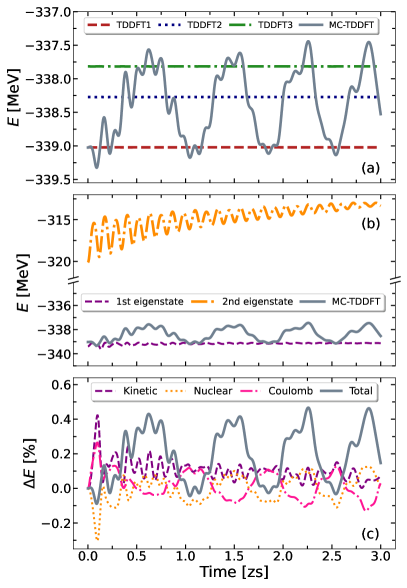
Figure 5: Energy conservation in the case of mixing of three TDDFT configurations, discussed in Sec. 5.3, for $(n=3,\Delta x_{1})$ and $\Delta t_{1}$. (a): Time evolution of energies of the TDDFT configurations and of the MC-TDDFT state. While TDDFT energies are constants of motion, the MC-TDDFT energy is not conserved. (b) Time evolution of the eigenvalues of the collective Hamiltonian and of the MC-TDDFT state. Note the break along the $y$-axis. The MC-TDDFT energy is bounded by the two eigenvalues. (c): Deviation, in percentage, of different components of the MC-TDDFT energy, $\Delta E_{i}=\Big{(}E_{i}(t)-E_{i}(0)\Big{)}/|E_{i}(0)|\cdot 100$. The kinetic, nuclear (Skyrme), and Coulomb component all contribute to the variation of the total energy.

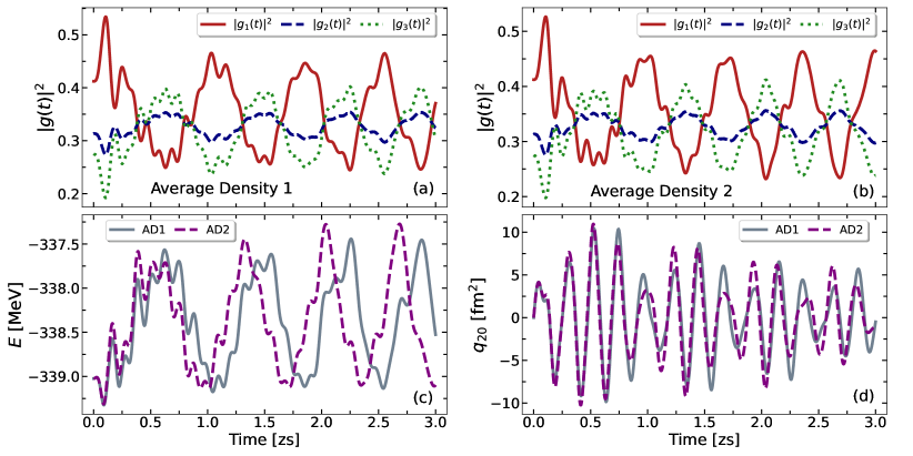
Figure 6: Influence of the choice of the density-dependent prescription in the case of mixing of three TDDFT configurations, discussed in Sec. 5.3, for $(n=3,\Delta x_{1})$ and $\Delta t_{1}$. (a): Squared modulus of the collective wave function with the AD1 prescription [Eq. (51)]. (b): Squared modulus of the collective wave function with the AD2 prescription [Eq. (52)]. (c): Comparison of the MC-TDDFT energy obtained with the two prescriptions. (d): Comparison of the isoscalar quadrupole moment of the MC-TDDFT state obtained with the two prescriptions.

To address the question of energy conservation within the MC-TDDFT framework, we consider the same example of mixing of three TDDFT configurations from the previous section. In Fig. 5(a), we show the time evolution of energies of the three TDDFT trajectories, as well as the energy of the MC-TDDFT state. As expected, the TDDFT energies are constant (up to numerical accuracy, see discussion in Sec. 5.1). On the other hand, the MC-TDDFT energy is markedly not a constant.

Due to the choice of initial conditions, at $t=0$ this energy corresponds to the energy of the first basis state. However, for $t>0$, the MC-TDDFT energy oscillates with the amplitude of about $1.5$ MeV. What may seem surprising at first glance is that these oscillations are not bounded by the TDDFT energies. In fact, it is straightforward to show that the amplitude of oscillations is limited by the eigenvalues of the collective Hamiltonian and not by the energies of the basis states.

Following Eq. (25), the MC-TDDFT energy can be calculated as

$$E_{\rm{MC-TDDFT}}(t)=g^{\dagger}(t)\mathcal{H}^{c}(t)g(t).$$ (69)

The collective Hamiltonian $\mathcal{H}^{c}(t)$ can be recast into the diagonal form,

$$\mathcal{H}^{c}(t)=U_{H}(t)\Lambda_{H}(t)U_{H}^{\dagger}(t).$$ (70)

Since the collective Hamiltonian matrix is Hermitian, $\Lambda_{H}(t)$ is a real and diagonal matrix of eigenvalues and $U_{H}(t)$ is the unitary matrix of eigenstates. Consequently, we have

$$E_{\rm{MC-TDDFT}}(t)=\tilde{g}^{\dagger}(t)\Lambda_{H}(t)\tilde{g}(t),$$ (71)

where $\tilde{g}(t)=U_{H}^{\dagger}(t)g(t)U_{H}(t)$. It then follows that the MC-TDDFT energy is bounded by the lowest and the highest eigenvalue of the collective Hamiltonian.

In Fig. 5(b), we show the time evolution of the eigenvalues of the collective Hamiltonian ($\dim_{k}=2$), alongside the energy of the mixed state. We verify that the MC-TDDFT energy is indeed bounded from below by the lowest eigenvalue of the collective Hamiltonian. Moreover, it never even approaches the upper limit, which is given by the second eigenvalue. This is consistent with the fact that the dynamics of the mixed state is largely driven by the dominant eigenstate of the collective Hamiltonian, with only minor admixtures of the other eigenstate.

To gain more insight into the energy of the mixed state, in Fig. 5(c) we show variations, in percentage, of different components of the MC-TDDFT energy. More precisely, we calculate $\Delta E_{i}=\Big{(}E_{i}(t)-E_{i}(0)\Big{)}/|E_{i}(0)|\cdot 100$, for $i=$ kinetic, nuclear (Skyrme), Coulomb. It is apparent that neither component alone is responsible for the variation of the total energy. Rather than that, variations in all components fluctuate with the magnitude of $<0.5\%$. It is worth noting that this implies that the variations are unlikely to stem from any issue related to the density-dependent prescription. Indeed, the kinetic energy, which is free from any such spuriosities, nevertheless exhibits comparable variations.

Actually, the non-conservation of energy appears to be a feature of multiconfigurational models that are not fully variational regnier2019 ; marevic2023 ; li2023 ; li2023b . These models are formulated under a simplifying assumption that the time evolution of each TDDFT trajectory can be performed independently, using the existing TDDFT solvers. While significantly alleviating the computational burden, such an approximation disregards the feedback between the evolution of the mixing function and the basis states, thus removing the mechanism that would enforce a strict energy conservation on the MC-TDDFT level. At best, the approximate energy conservation can be imposed by controlling the lower and the upper limit of the collective Hamiltonian eigenvalues. This is a clear shortcoming of such models, which can be understood as an intermediate step that renders the computational implementation feasible and enables pioneering exploration of the MC-TDDFT capabilities in atomic nuclei. Extending the model with a variational principle that treats both the mixing function and basis states as variational parameters, like in the toy model study of Ref. hasegawa2020 , is a natural method of ensuring the full energy conservation, at the price of explicitly including the effect of configuration mixing on individual TDDFT trajectories.

5.5 The density-dependent prescription

As mentioned in Sec. 3.2.3, a prescription is needed to evaluate the $\rho_{D}^{\alpha}(\bm{r})$ density in (44) and (50). To quantify the impact of this choice on the nuclear dynamics, we adopt the same example as in the previous two subsections. This time, however, we consider two different prescriptions for the density-dependent part of an effective interaction. In addition to the average density prescription of the form (51), which was used in all the calculations up to now, we also consider the prescription of the form (52). Both prescriptions yield real densities and reduce to the diagonal local density in the TDDFT limit. However, they are evidently not equivalent and some dependence of nuclear dynamics on this choice is, therefore, expected.

In Figs. 6(a) and 6(b), we compare the collective wave function obtained with the prescription (51) (”Average Density 1” - AD1) and the prescription (52) (”Average Density 2” - AD2). The main difference between the two panels appears to be a moderate shift in phase for larger values of $t$. Other than that, the overall dynamics seems relatively unaffected.

The impact on observables is examined in Figs. 6(c) and 6(d), where we compare the energy and the isoscalar quadrupole moment of the MC-TDDFT state, respectively, obtained with the two prescriptions. The amplitude of variations in energy remains very similar for the two prescriptions. On the other hand, there appears a moderate shift in phase, similar to the one seen in the collective wave function. Furthermore, the quadrupole moment is essentially unaffected up to $t\approx 0.75$ zs. Beyond this point, the difference in prescriptions starts to play a role, causing a moderate difference between the two curves.

One way to additionally quantify this difference is to calculate the excitation spectrum by performing a Fourier transform of the quadrupole response. In marevic2023 , we calculated this spectrum using the AD1 prescription and obtained the main giant resonance peak at about $18$ MeV, in agreement with experiments. Moreover, two additional peaks were observed at approximately twice and thrice the energy of the main peak, which were interpreted as multiphonon excitations of the main giant resonance. By repeating the same procedure for the response obtained with the AD2 prescription, we obtain essentially the same spectrum, with all the peaks shifted by less than $0.1$ MeV. This is an encouraging result, indicating that the main conclusions of marevic2023 may not be very sensible to the choice of density prescription.

6 Summary

The nuclear TDDFT framework is a tool of choice for describing various dynamical phenomena in atomic nuclei. However, it yields quasi-classical equations of motions in the collective space and, consequently, drastically understimates fluctuations of observables. On the other hand, the MC-TDDFT model encompasses both the dissipation and the quantum fluctuation aspects of nuclear dynamics within a fully quantum framework. Starting from a general mixing of diabatic many-body configurations, the time-dependent variational principle yields the equation of motion for the mixing function whose resolution provides an access to various observables of interest.

In Ref. marevic2023 , we reported a study of quadrupole oscillations in ⁴⁰Ca where several TDDFT configurations were mixed based on the Skyrme EDF framework. We demonstrated that the collective multiphonon states emerge at high excitation energies when quantum fluctuations in the collective space are included beyond the independent particle approximation. In this work, we provided more technical and numerical details of the underlying MC-TDDFT model.

The central equation of motion [Eq. (27)], obtained through a time-dependent variational principle with the mixing function as a variational parameter, describes a unitary time evolution of the collective wave function. We discussed methods for consistent computation of different ingredients of the equation, including the Hamiltonian kernel, norm kernel, and kernels with explicit time derivatives, as well as the choice of initial conditions and the direct resolution method. A special attention needs to be given when inverting the norm kernel matrix, since linear dependencies in the TDDFT basis can lead to numerical instabilities. Within the current implementation of the model, the TDDFT configurations are assumed to evolve independently. This approximation simplifies the problem significantly, but at the price of rendering the total energy a non-conserved quantity on the MC-TDDFT level. Furthermore, the density dependence of existing effective interactions requires employing a density prescription, which can be seen as an additional parameter of the model.

A technical discussion was supplemented with numerical examples, focusing on the issues of convergence, treatment of linearly dependent bases, energy conservation, and prescriptions for the density-dependent part of an effective interaction. To start with, we demonstrated the convergence of static and dynamic aspects of the new TDDFT solver, based on the finite element method. The time evolution of the MC-TDDFT state was shown to be unitary and well converged for a wide range of time steps and spatial meshes. Generally, finer spatial meshes require smaller time steps. Similarly, MC-TDDFT calculations require finer meshes than those used in TDDFT to achieve a comparable level of convergence. Linear dependencies in the basis need to be carefully treated, since including too small norm eigenvalues causes numerical instabilities, while excluding too large eigenvalues removes a part of physical information. The non-conservation of the MC-TDDFT energy is a combined effect of the kinetic, nuclear, and Coulomb components, and it is at the order of $0.5\%$ in the considered example. Finally, the two versions of the average density prescription discussed in this work yield only minor differences in the collective dynamics.

The very recent implementations of the MC-TDDFT framework in real nuclei marevic2023 ; li2023 ; li2023b , based on the pioneering work by Reinhard and collaborators reinhard1983 ; reinhard1987 and following the toy-model study of regnier2019 , have demonstrated the predictive power of the model. Further developments of the theoretical framework and computational methods are expected to render the model applicable to a wider range of nuclear phenomena in the near future. Future studies should also aim at elucidating the relation and difference in performance between the MC-TDDFT and the conventional TDGCM framework.

Appendix A Local transition densities

The spin expansion of the non-local transition density [Eq. (42)] for isospin $\tau$ reads

$$\begin{split}\rho_{\bm{q}\bm{q^{\prime}}}^{(\tau)}(\bm{r}\sigma,\bm{r^{\prime}}\sigma^{\prime};t)&=\frac{1}{2}\rho_{\bm{q}\bm{q^{\prime}}}^{(\tau)}(\bm{r},\bm{r^{\prime}};t)\delta_{\sigma\sigma^{\prime}}\\ &+\frac{1}{2}\sum_{\mu}\braket{\sigma}{\hat{\sigma}_{\mu}}{\sigma^{\prime}}s_{\bm{q}\bm{q^{\prime}},\mu}^{(\tau)}(\bm{r},\bm{r^{\prime}};t),\end{split}$$ (72)

where $\rho_{\bm{q}\bm{q^{\prime}}}^{(\tau)}(\bm{r},\bm{r^{\prime}};t)$ is the non-local one-body transition particle density,

$$\rho_{\bm{q}\bm{q^{\prime}}}^{(\tau)}(\bm{r},\bm{r^{\prime}};t)=\sum_{\sigma}\rho_{\bm{q}\bm{q^{\prime}}}^{(\tau)}(\bm{r}\sigma,\bm{r^{\prime}}\sigma;t),$$ (73)

$s_{\bm{q}\bm{q^{\prime}},\mu}^{(\tau)}(\bm{r},\bm{r^{\prime}};t)$ is the $\mu$-th component of the non-local one-body transition spin density,

$$s_{\bm{q}\bm{q^{\prime}},\mu}^{(\tau)}(\bm{r},\bm{r^{\prime}};t)=\sum_{\sigma\sigma^{\prime}}\rho_{\bm{q}\bm{q^{\prime}}}^{(\tau)}(\bm{r}\sigma,\bm{r^{\prime}}\sigma^{\prime};t)\braket{\sigma^{\prime}}{\hat{\sigma}_{\mu}}{\sigma},$$ (74)

and $\hat{\sigma}_{\mu}$ are the Pauli operators. The local variants of the particle density $\rho_{\bm{q}\bm{q^{\prime}}}^{(\tau)}(\bm{r};t)$, spin density $\bm{s}_{\bm{q}\bm{q^{\prime}}}^{(\tau)}(\bm{r};t)$, kinetic density $\tau_{\bm{q}\bm{q^{\prime}}}^{(\tau)}(\bm{r};t)$, current density $\bm{j}_{\bm{q}\bm{q^{\prime}}}^{(\tau)}(\bm{r};t)$, spin-current pseudotensor density $J_{\bm{q}\bm{q^{\prime}},\mu\nu}^{(\tau)}(\bm{r};t)$, and spin-orbit current vector density ${\rm{\bm{J}}}_{\bm{q}\bm{q^{\prime}}}^{(\tau)}(\bm{r};t)$ read

$$\rho_{\bm{q}\bm{q^{\prime}}}^{(\tau)}(\bm{r};t) =\rho_{\bm{q}\bm{q^{\prime}}}^{(\tau)}(\bm{r},\bm{r};t),$$ (75a)

$$s_{\bm{q}\bm{q^{\prime}},\mu}^{(\tau)}(\bm{r};t) =s_{\bm{q}\bm{q^{\prime}},\mu}^{(\tau)}(\bm{r},\bm{r};t),$$ (75b)

$$\tau_{\bm{q}\bm{q^{\prime}}}^{(\tau)}(\bm{r};t) =\nabla\cdot\nabla^{\prime}\rho_{\bm{q}\bm{q^{\prime}}}^{(\tau)}(\bm{r},\bm{r^{\prime}};t)|_{\bm{r^{\prime}}=\bm{r}},$$ (75c)

$$j_{\bm{q}\bm{q^{\prime}},\mu}^{(\tau)}(\bm{r};t) =\frac{1}{2i}(\nabla_{\mu}-\nabla^{\prime}_{\mu})\rho_{\bm{q}\bm{q^{\prime}}}^{(\tau)}(\bm{r},\bm{r^{\prime}};t)|_{\bm{r^{\prime}}=\bm{r}},$$ (75d)

$$J_{\bm{q}\bm{q^{\prime}},\mu\nu}^{(\tau)}(\bm{r};t) =\frac{1}{2i}(\nabla_{\mu}-\nabla^{\prime}_{\mu})s_{\bm{q}\bm{q^{\prime}},\nu}^{(\tau)}(\bm{r},\bm{r^{\prime}};t)|_{\bm{r^{\prime}}=\bm{r}},$$ (75e)

$${\rm{J}}_{\bm{q}\bm{q^{\prime}},\lambda}^{(\tau)}(\bm{r};t) =\sum_{\mu\nu}\epsilon_{\lambda\mu\nu}J_{\bm{q}\bm{q^{\prime}},\mu\nu}^{(\tau)}(\bm{r};t).$$ (75f)

In the following paragraph, the explicit dependence on time and isospin is omitted for compactness.

For Slater generating states, the coordinate space representation of the non-local transition density (for either neutrons or protons) can be written as

$$\rho_{\bm{q}\bm{q^{\prime}}}(\bm{r}\sigma,\bm{r^{\prime}}\sigma^{\prime})=\sum_{kl}\varphi_{k}^{\bm{q^{\prime}}}(\bm{r}\sigma)\Big{[}M_{\bm{q}\bm{q^{\prime}}}^{-1}\Big{]}_{kl}\varphi_{l}^{\bm{q}*}(\bm{r^{\prime}}\sigma^{\prime}),$$ (76)

where $\Big{[}M_{\bm{q}\bm{q^{\prime}}}^{-1}(t)\Big{]}_{kl}$ are (generally complex) elements of the inverted matrix of single-particle overlaps [Eq. (37)]. Given the decomposition (33), the local transition particle density reads

$$\rho_{\bm{q}\bm{q^{\prime}}}(\bm{r})=\sum_{kl}\Big{[}M_{\bm{q}\bm{q^{\prime}}}^{-1}\Big{]}_{kl}\Big{[}\rho_{\bm{q}\bm{q^{\prime}}}^{R}(\bm{r})+i\rho_{\bm{q}\bm{q^{\prime}}}^{I}(\bm{r})\Big{]}_{kl}$$ (77)

with

$$\Big{[}\rho_{\bm{q}\bm{q^{\prime}}}^{R}(\bm{r})\Big{]}_{kl} =\sum_{\alpha}\varphi_{k,\alpha}^{\bm{q^{\prime}}}(\bm{r})\varphi_{l,\alpha}^{\bm{q}}(\bm{r}),$$ (78a)

$$\Big{[}\rho_{\bm{q}\bm{q^{\prime}}}^{I}(\bm{r})\Big{]}_{kl} =\varphi_{k,1}^{\bm{q^{\prime}}}(\bm{r})\varphi_{l,0}^{\bm{q}}(\bm{r})-\varphi_{k,0}^{\bm{q^{\prime}}}(\bm{r})\varphi_{l,1}^{\bm{q}}(\bm{r})$$

$$+\varphi_{k,3}^{\bm{q^{\prime}}}(\bm{r})\varphi_{l,2}^{\bm{q}}(\bm{r})-\varphi_{k,2}^{\bm{q^{\prime}}}(\bm{r})\varphi_{l,3}^{\bm{q}}(\bm{r}),$$ (78b)

for $\alpha=0,1,2,3$. Similarly, the local transition kinetic density reads

$$\tau_{\bm{q}\bm{q^{\prime}}}(\bm{r})=\sum_{kl}\Big{[}M_{\bm{q}\bm{q^{\prime}}}^{-1}\Big{]}_{kl}\Big{[}\tau_{\bm{q}\bm{q^{\prime}}}^{R}(\bm{r})+i\tau_{\bm{q}\bm{q^{\prime}}}^{I}(\bm{r})\Big{]}_{kl},$$ (79)

with

$$\Big{[}\tau_{\bm{q}\bm{q^{\prime}}}^{R}(\bm{r})\Big{]}_{kl} =\sum_{\alpha}\big{(}\nabla\varphi_{k,\alpha}^{\bm{q^{\prime}}}(\bm{r})\big{)}\big{(}\nabla\varphi_{l,\alpha}^{\bm{q}}(\bm{r})\big{)},$$ (80a)

$$\Big{[}\tau_{\bm{q}\bm{q^{\prime}}}^{I}(\bm{r})\Big{]}_{kl} =\big{(}\nabla\varphi_{k,1}^{\bm{q^{\prime}}}(\bm{r})\big{)}\big{(}\nabla\varphi_{l,0}^{\bm{q}}(\bm{r})\big{)}$$

$$-\big{(}\nabla\varphi_{k,0}^{\bm{q^{\prime}}}(\bm{r})\big{)}\big{(}\nabla\varphi_{l,1}^{\bm{q}}(\bm{r})\big{)}$$

$$+\big{(}\nabla\varphi_{k,3}^{\bm{q^{\prime}}}(\bm{r})\big{)}\big{(}\nabla\varphi_{l,2}^{\bm{q}}(\bm{r})\big{)}$$

$$-\big{(}\nabla\varphi_{k,2}^{\bm{q^{\prime}}}(\bm{r})\big{)}\big{(}\nabla\varphi_{l,3}^{\bm{q}}(\bm{r})\big{)},$$ (80b)

with

$$\big{(}\nabla\varphi_{k,\alpha}^{\bm{q^{\prime}}}(\bm{r})\big{)}\big{(}\nabla\varphi_{l,\beta}^{\bm{q}}(\bm{r})\big{)}=\sum_{\mu}\big{(}\partial_{\mu}\varphi_{k,\alpha}^{\bm{q^{\prime}}}(\bm{r})\big{)}\big{(}\partial_{\mu}\varphi_{l,\beta}^{\bm{q}}(\bm{r})\big{)}$$ (81)

and $\mu=x,y,z$. Furthermore, the $\mu$-th component of the local transition current density reads

$$j_{\bm{q}\bm{q^{\prime}}}^{\mu}(\bm{r})=\frac{1}{2}\sum_{kl}\Big{[}M_{\bm{q}\bm{q^{\prime}}}^{-1}\Big{]}_{kl}\Big{[}j_{\bm{q}\bm{q^{\prime}}}^{\mu,R}(\bm{r})+ij_{\bm{q}\bm{q^{\prime}}}^{\mu,I}(\bm{r})\Big{]}_{kl},$$ (82)

with

$$\Big{[}j_{\bm{q}\bm{q^{\prime}}}^{\mu,R}(\bm{r})\Big{]}_{kl} =\big{(}\partial_{\mu}\varphi_{k,1}^{\bm{q^{\prime}}}(\bm{r})\big{)}\varphi_{l,0}^{\bm{q}}(\bm{r})-\big{(}\partial_{\mu}\varphi_{k,0}^{\bm{q^{\prime}}}(\bm{r})\big{)}\varphi_{l,1}^{\bm{q}}(\bm{r})$$

$$+\big{(}\partial_{\mu}\varphi_{k,3}^{\bm{q^{\prime}}}(\bm{r})\big{)}\varphi_{l,2}^{\bm{q}}(\bm{r})-\big{(}\partial_{\mu}\varphi_{k,2}^{\bm{q^{\prime}}}(\bm{r})\big{)}\varphi_{l,3}^{\bm{q}}(\bm{r})$$

$$-\varphi_{k,1}^{\bm{q^{\prime}}}(\bm{r})\big{(}\partial_{\mu}\varphi_{l,0}^{\bm{q}}(\bm{r})\big{)}+\varphi_{k,0}^{\bm{q^{\prime}}}(\bm{r})\big{(}\partial_{\mu}\varphi_{l,1}^{\bm{q}}(\bm{r})\big{)}$$

$$-\varphi_{k,3}^{\bm{q^{\prime}}}(\bm{r})\big{(}\partial_{\mu}\varphi_{l,2}^{\bm{q}}(\bm{r})\big{)}+\varphi_{k,2}^{\bm{q^{\prime}}}(\bm{r})\big{(}\partial_{\mu}\varphi_{l,3}^{\bm{q}}(\bm{r})\big{)},$$ (83a)

$$\Big{[}j_{\bm{q}\bm{q^{\prime}}}^{\mu,I}(\bm{r})\Big{]}_{kl} =\sum_{\alpha}\varphi_{k,\alpha}^{\bm{q^{\prime}}}(\bm{r})\big{(}\partial_{\mu}\varphi_{l,\alpha}^{\bm{q}}(\bm{r})\big{)}$$

$$-\sum_{\alpha}\big{(}\partial_{\mu}\varphi_{k,\alpha}^{\bm{q^{\prime}}}(\bm{r})\big{)}\varphi_{l,\alpha}^{\bm{q}}(\bm{r}),$$ (83b)

The components of the local transition spin density then read

$$s_{\bm{q}\bm{q^{\prime}}}^{\mu}(\bm{r})=\sum_{kl}\Big{[}M_{\bm{q}\bm{q^{\prime}}}^{-1}\Big{]}_{kl}\Big{[}s_{\bm{q}\bm{q^{\prime}}}^{\mu,R}(\bm{r})+is_{\bm{q}\bm{q^{\prime}}}^{\mu,I}(\bm{r})\Big{]}_{kl},$$ (84)

with

$$\Big{[}s_{\bm{q}\bm{q^{\prime}}}^{x,R}(\bm{r})\Big{]}_{kl} =\varphi_{k,0}^{\bm{q^{\prime}}}(\bm{r})\varphi_{l,2}^{\bm{q}}(\bm{r})+\varphi_{k,1}^{\bm{q^{\prime}}}(\bm{r})\varphi_{l,3}^{\bm{q}}(\bm{r})$$

$$+\varphi_{k,2}^{\bm{q^{\prime}}}(\bm{r})\varphi_{l,0}^{\bm{q}}(\bm{r})+\varphi_{k,3}^{\bm{q^{\prime}}}(\bm{r})\varphi_{l,1}^{\bm{q}}(\bm{r}),$$ (85a)

$$\Big{[}s_{\bm{q}\bm{q^{\prime}}}^{x,I}(\bm{r})\Big{]}_{kl} =\varphi_{k,1}^{\bm{q^{\prime}}}(\bm{r})\varphi_{l,2}^{\bm{q}}(\bm{r})-\varphi_{k,2}^{\bm{q^{\prime}}}(\bm{r})\varphi_{l,1}^{\bm{q}}(\bm{r})$$

$$+\varphi_{k,3}^{\bm{q^{\prime}}}(\bm{r})\varphi_{l,0}^{\bm{q}}(\bm{r})-\varphi_{k,0}^{\bm{q^{\prime}}}(\bm{r})\varphi_{l,3}^{\bm{q}}(\bm{r}),$$ (85b)

$$\Big{[}s_{\bm{q}\bm{q^{\prime}}}^{y,R}(\bm{r})\Big{]}_{kl} =\varphi_{k,0}^{\bm{q^{\prime}}}(\bm{r})\varphi_{l,3}^{\bm{q}}(\bm{r})+\varphi_{k,3}^{\bm{q^{\prime}}}(\bm{r})\varphi_{l,0}^{\bm{q}}(\bm{r})$$

$$-\varphi_{k,1}^{\bm{q^{\prime}}}(\bm{r})\varphi_{l,2}^{\bm{q}}(\bm{r})-\varphi_{k,2}^{\bm{q^{\prime}}}(\bm{r})\varphi_{l,1}^{\bm{q}}(\bm{r}),$$ (85c)

$$\Big{[}s_{\bm{q}\bm{q^{\prime}}}^{y,I}(\bm{r})\Big{]}_{kl} =\varphi_{k,0}^{\bm{q^{\prime}}}(\bm{r})\varphi_{l,2}^{\bm{q}}(\bm{r})-\varphi_{k,2}^{\bm{q^{\prime}}}(\bm{r})\varphi_{l,0}^{\bm{q}}(\bm{r})$$

$$+\varphi_{k,1}^{\bm{q^{\prime}}}(\bm{r})\varphi_{l,3}^{\bm{q}}(\bm{r})-\varphi_{k,3}^{\bm{q^{\prime}}}(\bm{r})\varphi_{l,1}^{\bm{q}}(\bm{r}),$$ (85d)

$$\Big{[}s_{\bm{q}\bm{q^{\prime}}}^{z,R}(\bm{r})\Big{]}_{kl} =\varphi_{k,0}^{\bm{q^{\prime}}}(\bm{r})\varphi_{l,0}^{\bm{q}}(\bm{r})+\varphi_{k,1}^{\bm{q^{\prime}}}(\bm{r})\varphi_{l,1}^{\bm{q}}(\bm{r})$$

$$-\varphi_{k,2}^{\bm{q^{\prime}}}(\bm{r})\varphi_{l,2}^{\bm{q}}(\bm{r})-\varphi_{k,3}^{\bm{q^{\prime}}}(\bm{r})\varphi_{l,3}^{\bm{q}}(\bm{r}),$$ (85e)

$$\Big{[}s_{\bm{q}\bm{q^{\prime}}}^{z,I}(\bm{r})\Big{]}_{kl} =\varphi_{k,1}^{\bm{q^{\prime}}}(\bm{r})\varphi_{l,0}^{\bm{q}}(\bm{r})-\varphi_{k,0}^{\bm{q^{\prime}}}(\bm{r})\varphi_{l,1}^{\bm{q}}(\bm{r})$$

$$+\varphi_{k,2}^{\bm{q^{\prime}}}(\bm{r})\varphi_{l,3}^{\bm{q}}(\bm{r})-\varphi_{k,3}^{\bm{q^{\prime}}}(\bm{r})\varphi_{l,2}^{\bm{q}}(\bm{r}).$$ (85f)

Finally, the components of the spin-current pseudotensor density read

$$J_{\bm{q}\bm{q^{\prime}}}^{\mu\nu}(\bm{r})=\frac{1}{2}\sum_{kl}\Big{[}M_{\bm{q}\bm{q^{\prime}}}^{-1}\Big{]}_{kl}\Big{[}J_{\bm{q}\bm{q^{\prime}}}^{\mu\nu,R}(\bm{r})+iJ_{\bm{q}\bm{q^{\prime}}}^{\mu\nu,I}(\bm{r})\Big{]}_{kl}$$ (86)

with

$$\Big{[}J_{\bm{q}\bm{q^{\prime}}}^{\mu x,R}(\bm{r})\Big{]}_{kl} =\big{(}\partial_{\mu}\varphi_{k,1}^{\bm{q^{\prime}}}(\bm{r})\big{)}\varphi_{l,2}^{\bm{q}}(\bm{r})-\varphi_{k,1}^{\bm{q^{\prime}}}(\bm{r})\big{(}\partial_{\mu}\varphi_{l,2}^{\bm{q}}(\bm{r})\big{)}$$

$$-\big{(}\partial_{\mu}\varphi_{k,0}^{\bm{q^{\prime}}}(\bm{r})\big{)}\varphi_{l,3}^{\bm{q}}(\bm{r})+\varphi_{k,0}^{\bm{q^{\prime}}}(\bm{r})\big{(}\partial_{\mu}\varphi_{l,3}^{\bm{q}}(\bm{r})\big{)}$$

$$+\big{(}\partial_{\mu}\varphi_{k,3}^{\bm{q^{\prime}}}(\bm{r})\big{)}\varphi_{l,0}^{\bm{q}}(\bm{r})-\varphi_{k,3}^{\bm{q^{\prime}}}(\bm{r})\big{(}\partial_{\mu}\varphi_{l,0}^{\bm{q}}(\bm{r})\big{)}$$

$$-\big{(}\partial_{\mu}\varphi_{k,2}^{\bm{q^{\prime}}}(\bm{r})\big{)}\varphi_{l,1}^{\bm{q}}(\bm{r})+\varphi_{k,2}^{\bm{q^{\prime}}}(\bm{r})\big{(}\partial_{\mu}\varphi_{l,1}^{\bm{q}}(\bm{r})\big{)},$$ (87a)

$$\Big{[}J_{\bm{q}\bm{q^{\prime}}}^{\mu x,I}(\bm{r})\Big{]}_{kl} =\varphi_{k,0}^{\bm{q^{\prime}}}(\bm{r})\big{(}\partial_{\mu}\varphi_{l,2}^{\bm{q}}(\bm{r})\big{)}-\big{(}\partial_{\mu}\varphi_{k,0}^{\bm{q^{\prime}}}(\bm{r})\big{)}\varphi_{l,2}^{\bm{q}}(\bm{r})$$

$$+\varphi_{k,1}^{\bm{q^{\prime}}}(\bm{r})\big{(}\partial_{\mu}\varphi_{l,3}^{\bm{q}}(\bm{r})\big{)}-\big{(}\partial_{\mu}\varphi_{k,1}^{\bm{q^{\prime}}}(\bm{r})\big{)}\varphi_{l,3}^{\bm{q}}(\bm{r})$$

$$+\varphi_{k,2}^{\bm{q^{\prime}}}(\bm{r})\big{(}\partial_{\mu}\varphi_{l,0}^{\bm{q}}(\bm{r})\big{)}-\big{(}\partial_{\mu}\varphi_{k,2}^{\bm{q^{\prime}}}(\bm{r})\big{)}\varphi_{l,0}^{\bm{q}}(\bm{r})$$

$$+\varphi_{k,3}^{\bm{q^{\prime}}}(\bm{r})\big{(}\partial_{\mu}\varphi_{l,1}^{\bm{q}}(\bm{r})\big{)}-\big{(}\partial_{\mu}\varphi_{k,3}^{\bm{q^{\prime}}}(\bm{r})\big{)}\varphi_{l,1}^{\bm{q}}(\bm{r}),$$ (87b)

$$\Big{[}J_{\bm{q}\bm{q^{\prime}}}^{\mu y,R}(\bm{r})\Big{]}_{kl} =\big{(}\partial_{\mu}\varphi_{k,0}^{\bm{q^{\prime}}}(\bm{r})\big{)}\varphi_{l,2}^{\bm{q}}(\bm{r})-\varphi_{k,0}^{\bm{q^{\prime}}}(\bm{r})\big{(}\partial_{\mu}\varphi_{l,2}^{\bm{q}}(\bm{r})\big{)}$$

$$+\big{(}\partial_{\mu}\varphi_{k,1}^{\bm{q^{\prime}}}(\bm{r})\big{)}\varphi_{l,3}^{\bm{q}}(\bm{r})-\varphi_{k,1}^{\bm{q^{\prime}}}(\bm{r})\big{(}\partial_{\mu}\varphi_{l,3}^{\bm{q}}(\bm{r})\big{)}$$

$$-\big{(}\partial_{\mu}\varphi_{k,2}^{\bm{q^{\prime}}}(\bm{r})\big{)}\varphi_{l,0}^{\bm{q}}(\bm{r})+\varphi_{k,2}^{\bm{q^{\prime}}}(\bm{r})\big{(}\partial_{\mu}\varphi_{l,0}^{\bm{q}}(\bm{r})\big{)}$$

$$-\big{(}\partial_{\mu}\varphi_{k,3}^{\bm{q^{\prime}}}(\bm{r})\big{)}\varphi_{l,1}^{\bm{q}}(\bm{r})+\varphi_{k,3}^{\bm{q^{\prime}}}(\bm{r})\big{(}\partial_{\mu}\varphi_{l,1}^{\bm{q}}(\bm{r})\big{)},$$ (87c)

$$\Big{[}J_{\bm{q}\bm{q^{\prime}}}^{\mu y,I}(\bm{r})\Big{]}_{kl} =\big{(}\partial_{\mu}\varphi_{k,1}^{\bm{q^{\prime}}}(\bm{r})\big{)}\varphi_{l,2}^{\bm{q}}(\bm{r})-\varphi_{k,1}^{\bm{q^{\prime}}}(\bm{r})\big{(}\partial_{\mu}\varphi_{l,2}^{\bm{q}}(\bm{r})\big{)}$$

$$-\big{(}\partial_{\mu}\varphi_{k,0}^{\bm{q^{\prime}}}(\bm{r})\big{)}\varphi_{l,3}^{\bm{q}}(\bm{r})+\varphi_{k,0}^{\bm{q^{\prime}}}(\bm{r})\big{(}\partial_{\mu}\varphi_{l,3}^{\bm{q}}(\bm{r})\big{)}$$

$$+\big{(}\partial_{\mu}\varphi_{k,2}^{\bm{q^{\prime}}}(\bm{r})\big{)}\varphi_{l,1}^{\bm{q}}(\bm{r})-\varphi_{k,2}^{\bm{q^{\prime}}}(\bm{r})\big{(}\partial_{\mu}\varphi_{l,1}^{\bm{q}}(\bm{r})\big{)}$$

$$-\big{(}\partial_{\mu}\varphi_{k,3}^{\bm{q^{\prime}}}(\bm{r})\big{)}\varphi_{l,0}^{\bm{q}}(\bm{r})+\varphi_{k,3}^{\bm{q^{\prime}}}(\bm{r})\big{(}\partial_{\mu}\varphi_{l,0}^{\bm{q}}(\bm{r})\big{)},$$ (87d)

$$\Big{[}J_{\bm{q}\bm{q^{\prime}}}^{\mu z,R}(\bm{r})\Big{]}_{kl} =\big{(}\partial_{\mu}\varphi_{k,1}^{\bm{q^{\prime}}}(\bm{r})\big{)}\varphi_{l,0}^{\bm{q}}(\bm{r})-\varphi_{k,1}^{\bm{q^{\prime}}}(\bm{r})\big{(}\partial_{\mu}\varphi_{l,0}^{\bm{q}}(\bm{r})\big{)}$$

$$-\big{(}\partial_{\mu}\varphi_{k,0}^{\bm{q^{\prime}}}(\bm{r})\big{)}\varphi_{l,1}^{\bm{q}}(\bm{r})+\varphi_{k,0}^{\bm{q^{\prime}}}(\bm{r})\big{(}\partial_{\mu}\varphi_{l,1}^{\bm{q}}(\bm{r})\big{)}$$

$$+\big{(}\partial_{\mu}\varphi_{k,2}^{\bm{q^{\prime}}}(\bm{r})\big{)}\varphi_{l,3}^{\bm{q}}(\bm{r})-\varphi_{k,2}^{\bm{q^{\prime}}}(\bm{r})\big{(}\partial_{\mu}\varphi_{l,3}^{\bm{q}}(\bm{r})\big{)}$$

$$-\big{(}\partial_{\mu}\varphi_{k,3}^{\bm{q^{\prime}}}(\bm{r})\big{)}\varphi_{l,2}^{\bm{q}}(\bm{r})+\varphi_{k,3}^{\bm{q^{\prime}}}(\bm{r})\big{(}\partial_{\mu}\varphi_{l,2}^{\bm{q}}(\bm{r})\big{)},$$ (87e)

$$\Big{[}J_{\bm{q}\bm{q^{\prime}}}^{\mu z,I}(\bm{r})\Big{]}_{kl} =\varphi_{k,0}^{\bm{q^{\prime}}}(\bm{r})\big{(}\partial_{\mu}\varphi_{l,0}^{\bm{q}}(\bm{r})\big{)}-\big{(}\partial_{\mu}\varphi_{k,0}^{\bm{q^{\prime}}}(\bm{r})\big{)}\varphi_{l,0}^{\bm{q}}(\bm{r})$$

$$+\varphi_{k,1}^{\bm{q^{\prime}}}(\bm{r})\big{(}\partial_{\mu}\varphi_{l,1}^{\bm{q}}(\bm{r})\big{)}-\big{(}\partial_{\mu}\varphi_{k,1}^{\bm{q^{\prime}}}(\bm{r})\big{)}\varphi_{l,1}^{\bm{q}}(\bm{r})$$

$$-\varphi_{k,2}^{\bm{q^{\prime}}}(\bm{r})\big{(}\partial_{\mu}\varphi_{l,2}^{\bm{q}}(\bm{r})\big{)}+\big{(}\partial_{\mu}\varphi_{k,2}^{\bm{q^{\prime}}}(\bm{r})\big{)}\varphi_{l,2}^{\bm{q}}(\bm{r})$$

$$-\varphi_{k,3}^{\bm{q^{\prime}}}(\bm{r})\big{(}\partial_{\mu}\varphi_{l,3}^{\bm{q}}(\bm{r})\big{)}+\big{(}\partial_{\mu}\varphi_{k,3}^{\bm{q^{\prime}}}(\bm{r})\big{)}\varphi_{l,3}^{\bm{q}}(\bm{r}).$$ (87f)

Appendix B Coupling constants

The coupling constants appearing in the Skyrme energy density (44) read

$$B_{1} =\frac{1}{2}t_{0}(1+\frac{1}{2}x_{0}),$$ (88a)

$$B_{2} =-\frac{1}{2}t_{0}(\frac{1}{2}+x_{0}),$$ (88b)

$$B_{3} =\frac{1}{4}\big{(}t_{1}(1+\frac{1}{2}x_{1})+t_{2}(1+\frac{1}{2}x_{2})\big{)},$$ (88c)

$$B_{4} =-\frac{1}{4}\big{(}t_{1}(\frac{1}{2}+x_{1})-t_{2}(\frac{1}{2}+x_{2})\big{)},$$ (88d)

$$B_{5} =-\frac{1}{16}\big{(}3t_{1}(1+\frac{1}{2}x_{1})-t_{2}(1+\frac{1}{2}x_{2})\big{)},$$ (88e)

$$B_{6} =\frac{1}{16}\big{(}3t_{1}(\frac{1}{2}+x_{1})+t_{2}(\frac{1}{2}+x_{2})\big{)},$$ (88f)

$$B_{7} =\frac{1}{12}t_{3}(1+\frac{1}{2}x_{3}),$$ (88g)

$$B_{8} =-\frac{1}{12}t_{3}(\frac{1}{2}+x_{3}),$$ (88h)

$$B_{9} =-\frac{1}{2}W,$$ (88i)

$$B_{10} =\frac{1}{4}t_{0}x_{0},$$ (88j)

$$B_{11} =-\frac{1}{4}t_{0},$$ (88k)

$$B_{12} =\frac{1}{24}t_{3}x_{3},$$ (88l)

$$B_{13} =-\frac{1}{24}t_{3}.$$ (88m)

Parameters $t_{i}$, $x_{i}$ ($i=0,1,2,3$), $W$, and $\alpha$ are the standard parameters of the Skyrme pseudopotential schunck2019 ; bonche1987 .

Appendix C Variance of a one-body operator in a normalized MC-TDDFT state

To evaluate the variance of Eq. (65), we need an expectation value of the $\hat{O}^{2}$ operator in a normalized MC-TDDFT state. We start from

$$\braket{\Psi(t)}{\hat{O}^{2}}{\Psi(t)}=\int_{\bm{q}\bm{q^{\prime}}}\!\!\,d\bm{q}\,d\bm{q^{\prime}}g^{*}_{\bm{q}}(t){\mathcal{O}^{2}}^{c}_{\bm{q}\bm{q^{\prime}}}(t)g_{\bm{q^{\prime}}}(t).$$ (89)

Again, the collective kernel of the $\hat{O}^{2}$ operator is calculated from (24) and the corresponding usual kernel follows from the generalized Wick theorem,

$$\begin{split}\mathcal{O}^{2}_{\bm{q}\bm{q^{\prime}}}(t)=\mathcal{N}_{\bm{q}\bm{q^{\prime}}}(t)\Big{[}&{\rm{Tr}}^{2}\big{(}O\rho^{\bm{q}\bm{q^{\prime}}}(t)\big{)}\\ +&{\rm{Tr}}\big{(}O\rho^{\bm{q}\bm{q^{\prime}}}(t)O(1-\rho^{\bm{q}\bm{q^{\prime}}}(t)\big{)}\Big{]}.\end{split}$$ (90)

Here,

$${\rm{Tr}}\big{(}O\rho^{\bm{q}\bm{q^{\prime}}}(t)\big{)}=\int\,d^{3}\bm{r}O(\bm{r})\rho_{\bm{q}\bm{q^{\prime}}}(\bm{r};t).$$ (91)

Furthermore, the second trace corresponds to the sum of two terms,

$${\rm{Tr}}\big{(}O\rho^{\bm{q}\bm{q^{\prime}}}(t)O(1-\rho^{\bm{q}\bm{q^{\prime}}}(t)\big{)}=C_{1}^{\bm{q}\bm{q^{\prime}}}(t)+C_{2}^{\bm{q}\bm{q^{\prime}}}(t).$$ (92)

The first term reads

$$\begin{split}C_{1}^{\bm{q}\bm{q^{\prime}}}(t)&=\int\,d^{3}\bm{r}O^{2}(\bm{r})\sum_{kl}\Big{[}M_{\bm{q}\bm{q^{\prime}}}^{-1}(t)\Big{]}_{kl}\\ &\times\biggl{\{}A_{kl}^{\bm{q}\bm{q^{\prime}}}(\bm{r};t)+iB_{kl}^{\bm{q}\bm{q^{\prime}}}(\bm{r};t)\biggl{\}},\end{split}$$ (93)

with

$$A_{kl}^{\bm{q}\bm{q^{\prime}}}(\bm{r};t)=\sum_{\alpha}\varphi_{k,\alpha}^{\bm{q^{\prime}}}(\bm{r};t)\varphi_{l,\alpha}^{\bm{q}}(\bm{r};t)$$ (94)

and

$$\begin{split}B_{kl}^{\bm{q}\bm{q^{\prime}}}(\bm{r};t)&=\varphi_{k,1}^{\bm{q^{\prime}}}(\bm{r};t)\varphi_{l,0}^{\bm{q}}(\bm{r};t)\\ &-\varphi_{k,0}^{\bm{q^{\prime}}}(\bm{r};t)\varphi_{l,1}^{\bm{q}}(\bm{r};t)\\ &+\varphi_{k,3}^{\bm{q^{\prime}}}(\bm{r};t)\varphi_{l,2}^{\bm{q}}(\bm{r};t)\\ &-\varphi_{k,2}^{\bm{q^{\prime}}}(\bm{r};t)\varphi_{l,3}^{\bm{q}}(\bm{r};t).\end{split}$$ (95)

The second term reads

$$\begin{split}C_{2}^{\bm{q}\bm{q^{\prime}}}(t)&=\int\,d^{3}\bm{r}\int\,d^{3}\bm{r^{\prime}}O(\bm{r})O(\bm{r^{\prime}})\\ &\times\sum_{klmn}\Big{[}M_{\bm{q}\bm{q^{\prime}}}^{-1}(t)\Big{]}_{kl}\Big{[}M_{\bm{q}\bm{q^{\prime}}}^{-1}(t)\Big{]}_{mn}\\ &\times\biggl{\{}A_{kn}^{\bm{q}\bm{q^{\prime}}}(\bm{r};t)+iB_{kn}^{\bm{q}\bm{q^{\prime}}}(\bm{r};t)\biggl{\}}\\ &\times\biggl{\{}A_{ml}^{\bm{q}\bm{q^{\prime}}}(\bm{r^{\prime}};t)+iB_{ml}^{\bm{q}\bm{q^{\prime}}}(\bm{r^{\prime}};t)\biggl{\}}.\end{split}$$ (96)

- (1) C. Simenel, B. Avez, D. Lacroix, Quantum Many-Body Dynamics: Applications to Nuclear Reactions, VDM Verlag, 2010.
- (2) D. Lacroix, S. Ayik, P. Chomaz, Nuclear collective vibrations in extended mean-field theory, Prog. Part. Nucl. Phys. 52 (2004) 497–563. doi:10.1016/j.ppnp.2004.02.002.
- (3) C. Simenel, Nuclear quantum many-body dynamics, Eur. Phys. J. A 48 (2012) 152. doi:10.1140/epja/i2012-12152-0.
- (4) A. Bulgac, Time-dependent density functional theory and the real-time dynamics of Fermi superfluids, Annu. Rev. Nucl. Part. Sci. 63 (2013) 97–121. doi:10.1146/annurev-nucl-102212-170631.
- (5) T. Nakatsukasa, K. Matsuyanagi, M. Matsuo, K. Yabana, Time-dependent density-functional description of nuclear dynamics, Rev. Mod. Phys. 88 (2016) 045004. doi:10.1103/RevModPhys.88.045004.
- (6) P. Stevenson, M. Barton, Low-energy heavy-ion reactions and the Skyrme effective interaction, Prog. Part. Nucl. Phys. 104 (2019) 142–164. doi:10.1016/j.ppnp.2018.09.002.
- (7) A. Bulgac, M. Forbes, ”Time-Dependent Density Functional Theory” (Chapter 4) in ”Energy Density Functional Methods for Atomic Nuclei” (Ed. Nicolas Schunck), IOP Publishing Ltd, 2019.
- (8) M. Casida, M. Huix-Rotllant, Progress in Time-Dependent Density-Functional Theory, Annu. Rev. Phys. Chem. 63 (2012) 287–323. doi:10.1146/annurev-physchem-032511-143803.
- (9) M. A. L. Marques, N. T. Maitra, F. Nogueira, E. K. U. Gross, A. Rubio (Eds.), Fundamentals of Time-Dependent Density Functional Theory, Springer, Berlin, 2012.
- (10) J.-P. Blaizot, G. Ripka, Quantum theory of finite systems, Vol. 3, MIT press Cambridge, MA, 1986.
- (11) P. Ring, P. Schuck, The nuclear many-body problem, Springer Science & Business Media, 2004.
- (12) N. N. Bogolyubov, J. Phys. (URSS) 10 (1946) 256.
- (13) H. Born, H. S. Green, A general kinetic theory of liquids I. The molecular distribution functions, Proc. R. Soc. A 188 (1946) 10–18. doi:10.1098/rspa.1946.0093.
- (14) J. G. Kirkwood, The Statistical Mechanical Theory of Transport Processes I. General Theory, J. Chem. Phys. 14 (1946) 180–201. doi:10.1063/1.1724117.
- (15) M. Bonitz, Quantum Kinetic Theory, Springer, Berlin, 2016.
- (16) F. Lackner, I. Březinová, T. Sato, K. L. Ishikawa, J. Burgdörfer, Propagating two-particle reduced density matrices without wave functions, Phys. Rev. A 91 (2015) 023412. doi:10.1103/PhysRevA.91.023412.
- (17) F. Lackner, I. Březinová, T. Sato, K. L. Ishikawa, J. Burgdörfer, High-harmonic spectra from time-dependent two-particle reduced-density-matrix theory, Phys. Rev. A 95 (2017) 033414. doi:10.1103/PhysRevA.95.033414.
- (18) K. Dietrich, J.-J. Niez, J.-F. Berger, Microscopic transport theory of nuclear processes, Nucl. Phys. A 832 (2010) 249–288. doi:10.1016/j.nuclphysa.2009.11.004.
- (19) R. Balian, M. Vénéroni, Fluctuations in a time-dependent mean-field approach, Phys. Lett. B 136 (1984) 301–306. doi:10.1016/0370-2693(84)92008-2.
- (20) R. Balian, M. Vénéroni, Correlations and fluctuations in static and dynamic mean-field approaches, Ann. Phys. (N. Y.) 216 (1992) 351–430. doi:10.1016/0003-4916(92)90181-K.
- (21) C. Simenel, Particle-Number Fluctuations and Correlations in Transfer Reactions Obtained Using the Balian-Vénéroni Variational Principle, Phys. Rev. Lett. 106 (2011) 112502. doi:10.1103/PhysRevLett.106.112502.
- (22) P.-G. Reinhard, E. Suraud, Stochastic TDHF and large fluctuations, Nucl. Phys. A 545 (1992) 59–69. doi:10.1016/0375-9474(92)90446-Q.
- (23) P.-G. Reinhard, E. Suraud, Stochastic TDHF and the Boltzman-Langevin equation, Ann. Phys. (N. Y.) 216 (1992) 98–121. doi:10.1016/0003-4916(52)90043-2.
- (24) D. Lacroix, Stochastic mean-field dynamics for fermions in the weak-coupling limit, Phys. Rev. C 73 (2006) 044311. doi:10.1103/PhysRevC.73.044311.
- (25) S. Ayik, A stochastic mean-field approach for nuclear dynamics, Phys. Lett. B 658 (2008) 174–179. doi:10.1016/j.physletb.2007.09.072.
- (26) D. Lacroix, S. Ayik, Stochastic quantum dynamics beyond mean field, Eur. Phys. J. A 50 (2014) 95. doi:10.1140/epja/i2014-14095-8.
- (27) O. Juillet, P. Chomaz, Exact Stochastic Mean-Field Approach to the Fermionic Many-Body Problem, Phys. Rev. Lett. 88 (2002) 142503. doi:10.1103/PhysRevLett.88.142503.
- (28) D. Lacroix, Exact and approximate many-body dynamics with stochastic one-body density matrix evolution, Phys. Rev. C 71 (2005) 064322. doi:10.1103/PhysRevC.71.064322.
- (29) Y. Tanimura, D. Lacroix, S. Ayik, Microscopic Phase-Space Exploration Modeling of Spontaneous Fission, Phys. Rev. Lett. 118 (2017) 152501. doi:10.1103/PhysRevLett.118.152501.
- (30) D. Regnier, D. Lacroix, G. Scamps, Y. Hashimoto, Microscopic description of pair transfer between two superfluid Fermi systems: Combining phase-space averaging and combinatorial techniques, Phys. Rev. C 97 (2018) 034627. doi:10.1103/PhysRevC.97.034627.
- (31) D. Regnier, D. Lacroix, Microscopic description of pair transfer between two superfluid Fermi systems. II. Quantum mixing of time-dependent Hartree-Fock-Bogolyubov trajectories, Phys. Rev. C 99 (2019) 064615. doi:10.1103/PhysRevC.99.064615.
- (32) M. Bender, P.-H. Heenen, P.-G. Reinhard, Self-consistent mean-field models for nuclear structure, Rev. Mod. Phys. 75 (2003) 121–180. doi:10.1103/RevModPhys.75.121.
- (33) J. L. Egido, State-of-the-art of beyond mean field theories with nuclear density functionals, Phys. Scr. 91 (2016) 073003. doi:10.1088/0031-8949/91/7/073003.
- (34) L. M. Robledo, T. R. Rodríguez, R. R. Rodríguez-Guzmán, Mean field and beyond description of nuclear structure with the Gogny force: a review, J. Phys. G: Nucl. Part. Phys. 46 (2018) 013001. doi:10.1088/1361-6471/aadebd.
- (35) T. Nikšić, D. Vretenar, P. Ring, Relativistic nuclear energy density functionals: Mean-field and beyond, Prog. Part. Nucl. Phys. 66 (2011) 519–548. doi:10.1016/j.ppnp.2011.01.055.
- (36) J.-F. Berger, M. Girod, D. Gogny, Microscopic analysis of collective dynamics in low energy fission, Nucl. Phys. A 428 (1984) 23–36. doi:https://doi.org/10.1016/0375-9474(84)90240-9.
- (37) H. Goutte, P. Casoli, J.-F. Berger, Mass and kinetic energy distributions of fission fragments using the time dependent generator coordinate method, Nucl. Phys. A 734 (2004) 217–220. doi:10.1016/j.nuclphysa.2004.01.038.
- (38) W. Younes, D. M. Gogny, J.-F. Berger, A Microscopic Theory of Fission Dynamics Based on the Generator Coordinate Method, Springer Cham, 2019.
- (39) M. Verriere, D. Regnier, The time-dependent generator coordinate method in nuclear physics, Front. Phys. 8 (2020) 233. doi:10.3389/fphy.2020.00233.
- (40) D. Brink, A. Weiguny, The generator coordinate theory of collective motion, Nucl. Phys. A 120 (1968) 59–93. doi:10.1016/0375-9474(68)90059-6.
- (41) N. Onishi, T. Une, Local Gaussian Approximation in the Generator Coordinate Method, Prog. Theor. Phys. 53 (1975) 504–515. doi:10.1143/PTP.53.504.
- (42) D. Regnier, N. Dubray, N. Schunck, M. Verrière, Fission fragment charge and mass distributions in in the adiabatic nuclear energy density functional theory, Phys. Rev. C 93 (2016) 054611. doi:10.1103/PhysRevC.93.054611.
- (43) N. Schunck, L. M. Robledo, Microscopic theory of nuclear fission: a review, Rep. Prog. Phys. 79 (2016) 116301. doi:10.1088/0034-4885/79/11/116301.
- (44) M. Bender, R. Bernard, G. Bertsch, S. Chiba, J. Dobaczewski, N. Dubray, S. A. Giuliani, K. Hagino, D. Lacroix, Z. Li, P. Magierski, J. Maruhn, W. Nazarewicz, J. Pei, S. Péru, N. Pillet, J. Randrup, D. Regnier, P.-G. Reinhard, L. M. Robledo, W. Ryssens, J. Sadhukhan, G. Scamps, N. Schunck, C. Simenel, J. Skalski, I. Stetcu, P. Stevenson, S. Umar, M. Verriere, D. Vretenar, M. Warda, S. Åberg, Future of nuclear fission theory, J. Phys. G: Nucl. Part. Phys. 47 (2020) 113002. doi:10.1088/1361-6471/abab4f.
- (45) J. Zhao, T. Nikšić, D. Vretenar, Time-dependent generator coordinate method study of fission: Dissipation effects, Phys. Rev. C 105 (2022) 054604. doi:10.1103/PhysRevC.105.054604.
- (46) J. Zhao, T. Nikšić, D. Vretenar, Time-dependent generator coordinate method study of fission. II. Total kinetic energy distribution, Phys. Rev. C 106 (2022) 054609. doi:10.1103/PhysRevC.106.054609.
- (47) R. Bernard, H. Goutte, D. Gogny, W. Younes, Microscopic and nonadiabatic Schrödinger equation derived from the generator coordinate method based on zero- and two-quasiparticle states, Phys. Rev. C 84 (2011) 044308. doi:10.1103/PhysRevC.84.044308.
- (48) P.-G. Reinhard, R. Y. Cusson, K. Goeke, Time evolution of coherent ground-state correlations and the TDHF approach, Nucl. Phys. A 398 (1983) 141–188. doi:https://doi.org/10.1016/0375-9474(83)90653-X.
- (49) P. G. Reinhard, K. Goeke, The generator coordinate method and quantised collective motion in nuclear systems, Rep. Prog. Phys. 50 (1987) 1. doi:10.1088/0034-4885/50/1/001.
- (50) N. Hasegawa, K. Hagino, Y. Tanimura, Time-dependent generator coordinate method for many-particle tunneling, Phys. Lett. B 808 (2020) 135693. doi:10.1016/j.physletb.2020.135693.
- (51) A. Ono, Phase-space consideration on barrier transmission in a time-dependent variational approach with superposed wave packets, Phys. Lett. B 826 (2022) 136931. doi:10.1016/j.physletb.2022.136931.
- (52) N. Hasegawa, K. Hagino, Y. Tanimura, Comment on ”Phase-space consideration on barrier transmission in a time-dependent variational approach with superposed wave packets” (2022). arXiv:2202.00513.
- (53) A. Ono, Reply to Comment on ”Phase-space consideration on barrier transmission in a time-dependent variational approach with superposed wave packets” (2022). arXiv:2202.06454.
- (54) P. Marević, D. Regnier, D. Lacroix, Quantum fluctuations induce collective multiphonons in finite Fermi liquids, Phys. Rev. C 108 (2023) 014620. doi:10.1103/PhysRevC.108.014620.
- (55) B. Li, D. Vretenar, T. Nikšić, P. W. Zhao, J. Meng, Generalized time-dependent generator coordinate method for small- and large-amplitude collective motion, Phys. Rev. C 108 (2023) 014321. doi:10.1103/PhysRevC.108.014321.
- (56) B. Li, D. Vretenar, T. Nikšić, J. Zhao, P. W. Zhao, J. Meng, Generalized time-dependent generator coordinate method for small and large amplitude collective motion (ii): pairing correlations and fission (2023). arXiv:2309.12564.
- (57) D. L. Hill, J. A. Wheeler, Nuclear Constitution and the Interpretation of Fission Phenomena, Phys. Rev. 89 (1953) 1102–1145. doi:10.1103/PhysRev.89.1102.
- (58) J. J. Griffin, J. A. Wheeler, Collective Motions in Nuclei by the Method of Generator Coordinates, Phys. Rev. 108 (1957) 311–327. doi:10.1103/PhysRev.108.311.
- (59) J. A. Sheikh, J. Dobaczewski, P. Ring, L. M. Robledo, C. Yannouelas, Symmetry restoration in mean-field approaches, J. Phys. G: Nucl. Part. Phys. 48 (2019) 123001. doi:10.1088/1361-6471/ac288a.
- (60) J. Sadhukhan, J. Dobaczewski, W. Nazarewicz, J. A. Sheikh, A. Baran, Pairing-Induced Speedup of Nuclear Spontaneous Fission, Phys. Rev. C 90 (2014) 061304. doi:10.1103/PhysRevC.90.061304.
- (61) J. Zhao, B.-N. Lu, T. Nikšić, D. Vretenar, S.-G. Zhou, Multidimensionally-constrained relativistic mean-field study of spontaneous fission: Coupling between shape and pairing degrees of freedom, Phys. Rev. C 93 (2016) 044315. doi:10.1103/PhysRevC.93.044315.
- (62) R. Bernard, S. A. Giuliani, L. M. Robledo, Role of dynamic pairing correlations in fission dynamics, Phys. Rev. C 99 (2019) 064301. doi:10.1103/PhysRevC.99.064301.
- (63) H.-D. Meyer, F. Gatti, G. A. Worth, Multidimensional Quantum Dynamics: MCTDH Theory and Applications, John Wiley & Sons, 2009.
- (64) X. Yuan, S. Endo, Q. Zhao, Y. Li, S. C. Benjamin, Theory of variational quantum simulation, Quantum 3 (2019) 191. doi:10.22331/q-2019-10-07-191.
- (65) Y. Saad, Iterative Methods for Sparse Linear Systems: Second Edition, SIAM, 2003.
- (66) P.-O. Löwdin, Quantum Theory of Many-Particle Systems. I. Physical Interpretations by Means of Density Matrices, Natural Spin-Orbitals, and Convergence Problems in the Method of Configurational Interaction, Phys. Rev. 97 (1955) 1474–1489. doi:10.1103/PhysRev.97.1474.
- (67) F. Plasser, M. Ruckenbauer, S. Mai, M. Oppel, P. Marquetand, L. González, Efficient and Flexible Computation of Many-Electron Wave Function Overlaps, J. Chem. Theory Comput. 12 (2016) 1207–1219. doi:10.1021/acs.jctc.5b01148.
- (68) R. Balian, E. Brezin, Nonunitary Bogoliubov transformations and extension of Wick’s theorem, Il Nuovo Cimento B 64 (1969) 37–55. doi:10.1007/BF02710281.
- (69) M. Anguiano, J. Egido, L. Robledo, Particle number projection with effective forces, Nucl. Phys. A 696 (2001) 467–493. doi:https://doi.org/10.1016/S0375-9474(01)01219-2.
- (70) J. Dobaczewski, M. V. Stoitsov, W. Nazarewicz, P.-G. Reinhard, Particle-number projection and the density functional theory, Phys. Rev. C 76 (2007) 054315. doi:10.1103/PhysRevC.76.054315.
- (71) T. Duguet, M. Bender, K. Bennaceur, D. Lacroix, T. Lesinski, Particle-number restoration within the energy density functional formalism: Nonviability of terms depending on noninteger powers of the density matrices, Phys. Rev. C 79 (2009) 044320. doi:10.1103/PhysRevC.79.044320.
- (72) L. M. Robledo, Remarks on the use of projected densities in the density-dependent part of Skyrme or Gogny functionals, J. Phys. G: Nucl. Part. Phys. 37 (2010) 064020. doi:10.1088/0954-3899/37/6/064020.
- (73) P. Bonche, H. Flocard, P. Heenen, Self-consistent calculation of nuclear rotations: The complete yrast line of 24Mg, Nucl. Phys. A 467 (1987) 115–135. doi:10.1016/0375-9474(87)90331-9.
- (74) T. Duguet, P. Bonche, Density dependence of two-body interactions for beyond–mean-field calculations, Phys. Rev. C 67 (2003) 054308. doi:10.1103/PhysRevC.67.054308.
- (75) R. Bhatia, Matrix Analysis, Springer-Verlag, New York, 1997.
- (76) O. C. Zienkiewicz, R. L. Taylor, The Finite Element Method: Its Basis and Fundamentals, 7th Edition, Butterworth-Heinemann, Amsterdam, 2013.
- (77) R. Anderson, J. Andrej, A. Barker, J. Bramwell, J.-S. Camier, J. C. V. Dobrev, Y. Dudouit, A. Fisher, T. Kolev, W. Pazner, M. Stowell, V. Tomov, I. Akkerman, J. Dahm, D. Medina, S. Zampini, MFEM: A modular finite element methods library, Comput. Math. with Appl. 81 (2021) 42–74. doi:10.1016/j.camwa.2020.06.009.
- (78) K.-H. Kim, T. Otsuka, P. Bonche, Three-dimensional TDHF calculations for reactions of unstable nuclei, J. Phys. G: Nucl. Part. Phys. 23 (1997) 1267. doi:10.1088/0954-3899/23/10/014.
- (79) P. Marević, N. Schunck, E. Ney, R. Navarro Pérez, M. Verriere, J. O’Neal, Axially-deformed solution of the Skyrme-Hartree-Fock-Bogoliubov equations using the transformed harmonic oscillator basis (IV) HFBTHO (v4.0): A new version of the program, Comput. Phys. Commun. 276 (2022) 108367. doi:10.1016/j.cpc.2022.108367.
- (80) G. Scamps, D. Lacroix, Systematics of isovector and isoscalar giant quadrupole resonances in normal and superfluid spherical nuclei, Phys. Rev. C 88 (2013) 044310. doi:10.1103/PhysRevC.88.044310.
- (81) B. Schuetrumpf, P. G. Reinhard, P. D. Stevenson, A. S. Umar, J. A. Maruhn, The TDHF code Sky3D version 1.1, Comput. Phys. Commun. 229 (2018) 211–213. doi:10.1016/j.cpc.2018.03.012.
- (82) S. Jin, K. J. Roche, I. Stetcu, I. Abdurrahman, A. Bulgac, The LISE package: Solvers for static and time-dependent superfluid local density approximation equations in three dimensions, Comput. Phys. Commun. 269 (2021) 108130. doi:10.1016/j.cpc.2021.108130.
- (83) P. Chomaz, N. Frascaria, Multiple phonon excitation in nuclei: experimental results and theoretical descriptions, Phys. Rep. 252 (1995) 275–405. doi:10.1016/0370-1573(94)00079-I.
- (84) T. Aumann, P. F. Bortignon, H. Emling, Multiphonon giant resonances in nuclei, Annu. Rev. Nucl. Part. Sci. 48 (1998) 351–399. doi:10.1146/annurev.nucl.48.1.351.