Information-theoretic causality and applications to turbulence: energy cascade and inner/outer layer interactions

Abstract

We introduce an information-theoretic method for quantifying causality in chaotic systems. The approach, referred to as IT-causality, quantifies causality by measuring the information gained about future events conditioned on the knowledge of past events. The causal interactions are classified into redundant, unique, and synergistic contributions depending on their nature. The formulation is non-intrusive, invariance under invertible transformations of the variables, and provides the missing causality due to unobserved variables. The method only requires pairs of past-future events of the quantities of interest, making it convenient for both computational simulations and experimental investigations. IT-causality is validated in four scenarios representing basic causal interactions among variables: mediator, confounder, redundant collider, and synergistic collider. The approach is leveraged to address two questions relevant to turbulence research: i) the scale locality of the energy cascade in isotropic turbulence, and ii) the interactions between inner and outer layer flow motions in wall-bounded turbulence. In the former case, we demonstrate that causality in the energy cascade flows sequentially from larger to smaller scales without requiring intermediate scales. Conversely, the flow of information from small to large scales is shown to be redundant. In the second problem, we observe a unidirectional causality flow, with causality predominantly originating from the outer layer and propagating towards the inner layer, but not vice versa. The decomposition of IT-causality into intensities also reveals that the causality is primarily associated with high-velocity streaks. The Python scripts to compute IT-causality can be found here.

1 Introduction

Causality is the mechanism through which one event contributes to the genesis of another (Pearl, 2009). Causal inference stands as a cornerstone in the pursuit of scientific knowledge (Bunge, 2017): it is via the exploration of cause-and-effect relationships that we are able to gain understanding of a given phenomenon and to shape the course of events by deliberate actions. Despite its ubiquity, the adoption of specialized tools tailored for unraveling causal relationships remains limited within the turbulence community. In this work, we propose a non-intrusive method for quantification of causality formulated within the framework of information theory.

Causality in turbulence research is commonly inferred from a combination of numerical and experimental data interrogation. The tools encompass diverse techniques such as statistical analysis, energy budgets, linear and nonlinear stability theory, coherent structure analysis, and modal decomposition, to name a few (e.g. Robinson, 1991; Reed et al., 1996; Cambon & Scott, 1999; Schmid, 2007; Smits et al., 2011; Jiménez, 2012; Kawahara et al., 2012; Mezić, 2013; Haller, 2015; Wallace, 2016; Jiménez, 2018; Marusic & Monty, 2019). Additional research strategies involve the use of time cross-correlation between pairs of time signals representing events of interest as a surrogate for causal inference. For instance, investigations into turbulent kinetic energy (Jiménez, 2018; Cardesa et al., 2015) and the spatiotemporal aspects of spectral quantities (e.g., Choi & Moin, 1990; Wallace, 2014; Wilczek et al., 2015; de Kat & Ganapathisubramani, 2015; He et al., 2017; Wang et al., 2020) exemplify some of these efforts. However, it is known that correlation, while informative, does not inherently imply causation as it lacks the directionality and asymmetry required to quantify causal interactions (Beebee et al., 2012). While the aforementioned tools have significantly advanced our physical understanding of turbulence, extracting rigorous causal relationships from the current methodologies remains a challenging task.

An alternative and intuitive definition of causality is rooted in the concept of interventions: the manipulation of the causing variable results in changes in the effect (Pearl, 2009; Eichler, 2013). Interventions provide a pathway for evaluating the causal impact that one process $A$ exerts on another process $B$. This is achieved by adjusting $A$ to a modified value $\widetilde{A}$ and subsequently observing the post-intervention consequences on $B$. Within the turbulence literature, there are numerous examples where the equations of motion are modified to infer causal interactions within the system (e.g. Jiménez & Moin, 1991; Jiménez & Pinelli, 1999; Hwang & Cossu, 2010; Farrell et al., 2017; Lozano-Durán et al., 2021, to name a few). Despite the intuitiveness of interventions as a measure of causality, this approach is not without limitations (Eberhardt & Scheines, 2007). Causality with interventions is intrusive (i.e., it requires modifying the system) and costly (simulations need to be recomputed for numerical experiments). When data is gathered from physical experiments, establishing causality through interventions can be even more challenging or impractical (for example, in a wind tunnel setup). Additionally, the concept of causality with interventions prompts questions about the type of intervention that must be introduced and whether this intervention could impact the outcome of the exercise as a consequence of forcing the system out of its natural attractor.

The framework of information theory, the science of message communication (Shannon, 1948), provides an alternative, non-intrusive definition of causality as the information transferred from the variable $A$ to the variable $B$. The origin of this idea can be traced back to the work of Wiener (1956), and its initial quantification was presented by Granger (1969) through signal forecasting using linear autoregressive models. In the domain of information theory, this definition was formally established by Massey (1990) and Kramer (1998) through the utilization of conditional entropies, employing what is known as directed information. Building upon the direction of information flow in Markov chains, Schreiber (2000) introduced a heuristic definition of causality termed transfer entropy. In a similar vein, Liang & Kleeman (2006) and subsequently Sinha & Vaidya (2016) suggested inferring causality by measuring the information flow within a dynamical system when one variable is momentarily held constant for infinitesimally small times. More recently, Lozano-Durán & Arranz (2022) proposed a new information-theoretic quantification of causality for multivariate systems that generalizes the definition of transfer entropy. Other methods have been proposed for causal discovery beyond the framework of information theory. These include nonlinear state-space reconstruction based on Takens’ theorem (Arnhold et al., 1999; Sugihara et al., 2012), conditional independence-based methods (Runge et al., 2018; Runge, 2018), restricted Perron-Frobenius operator (Jiménez, 2023), reconstruction of causal graphs and Bayesian networks (Rubin, 1974; Spirtes et al., 2000; Pearl, 2000; Koller & Friedman, 2009; Imbens & Rubin, 2015). Runge et al. (2019) offers an overview of the methods for causal inference in the context of Earth system sciences. The reader is also referred to Camps-Valls et al. (2023) for a comprehensive summary of causality tools across disciplines.

The development and application of causality tools in the realm of turbulence research remain scarce. Among the current studies, we can cite the work by Tissot et al. (2014), who used Granger causality to investigate the dynamics of self-sustaining wall-bounded turbulence. Materassi et al. (2014) used normalized transfer entropy to study the cascading process in synthetic turbulence generated via the shell model. Liang & Lozano-Durán (2016) and Lozano-Durán et al. (2019) applied information-theoretic definitions of causality to unveil the dynamics of energy-containing eddies in wall-bounded turbulence. A similar approach was followed by Wang et al. (2021) and Wang et al. (2022) to study cause-and-effect interactions in turbulent flows over porous media. Lozano-Durán & Arranz (2022) used information flux among variables to study the energy cascade in isotropic turbulence. Recently, Martínez-Sánchez et al. (2023) used transfer entropy to analyze the formation mechanisms of large-scale coherent structures in the flow around a wall-mounted square cylinder. The new method proposed here to quantify causality addresses important deficiencies compared to existing tools in the literature.

This work is organized as follows. First, we discuss key aspects of causal inference in §1.1. The method is introduced in §2. The fundamentals of information theory required to formulate the problem of IT-causality are presented in §2.1 and the method is introduced in §2.2 along with a simple example and a discussion of its properties. The approach is validated in simple stochastic systems in §3. IT-causality is used to investigate two important problems in turbulence: the locality in scale of the energy cascade (§4); and the interaction between flow motions in the inner layer and outer layer of wall-bounded turbulence (§5). Finally, limitations of the method are outlined in §6 and conclusion are offered in §7.

1.1 Key concepts in causal inference

We discuss the distinction between causality, association, and correlation, as well as descriptions of the three basic categories of interactions between variables: mediator, confounder, and collider. These are well-established concepts in the field of causal inference (see, for example Pearl, 2009), yet they remain relatively underutilized within the turbulence research community.

Causality refers to the process by which one variable directly influences or determines changes in another variable. In causal relationships, a modification in the cause leads to a corresponding alteration in the effect, and there is a logical and temporal connection between them. For example, the rainy season in a particular region is a cause of increased umbrella sales. On the other hand, association signifies a statistical connection between two variables where they tend to occur together more frequently than expected by chance. Association does not necessarily imply causation; it could result from common causes, statistical coincidences, or confounding factors. One example of association is the increase in umbrella sales and raincoat sales, which tends to happen concurrently due to the confounding factor of the rainy season. Correlation is a specific form of association that quantifies the strength and direction of a linear (Pearson, 1895) or monotonic (Spearman, 1987) relationship between two variables. Correlation does not imply causation and can even fail to identify associations. In general, correlation implies association but not causation. Causation implies association but not correlation (Altman & Krzywinski, 2015).

Another crucial factor to consider is the manner variables interact. Let us consider three variables: $A$, $B$, and $C$. We can identify three fundamental types of interactions as summarized in figure 1.

• Mediator variables emerge in the causal chain from $A$ to $C$, with the variable $B$ acting as a bridge: $A\rightarrow B\rightarrow C$. In this scenario, $B$ is often viewed as the mechanism or mediator responsible for transmitting the influence of $A$ to $C$. Mediator variables help explain the underlying mechanisms by which an independent variable influences a dependent variable. A simple example is $\uparrow$ education level $\rightarrow$ $\uparrow$ job skills $\rightarrow$ $\uparrow$ income.

• Confounder variables serve as a common cause for two variables: $B\rightarrow A$ and $B\rightarrow C$. Confounder variables have the potential to create a statistical correlation between $A$ and $C$, even if there is no direct causal link between them. Consequently, confounding variables are factors that can obscure or distort the genuine relationship between variables. Following the example above, rainy season $\rightarrow$ $\uparrow$ umbrella sales and rainy season $\rightarrow$ $\uparrow$ raincoat sales.

• Collider variables are caused by the effect of multiple variables: $A\rightarrow B$ and $C\rightarrow B$. This scenario is particularly relevant in chaotic dynamical systems, where most variables are affected by multiple causes due to non-linear coupling.

  • A collider variable exhibits redundant causes when both $A$ and $C$ contribute to the same effect or outcome of $B$, creating overlapping or duplicative influences on the outcome. Consequently, redundant causes result in multiple pathways to the same effect. For instance, both hard work and high intelligence can independently contribute to the good grades of a student. Note that $A$ and $C$ may not necessarily be independent.

  • A collider variable is caused from synergistic variables if the combined effect of $A$ and $C$ on $B$ surpasses their individual effects on $B$ when considered separately. As an example, two drugs may be required in tandem to effectively treat a condition; when each drug alone is insufficient.

Figure 1: Schematic representation of mediator, confounder, and collider variables.

The interactions described above can combine and occur simultaneously, giving rise to more intricate causal networks. The method proposed below aims to distinguish between these various interactions, provided that we have sufficient knowledge of the system.

2 Method formulation

2.1 Fundamentals of information theory

Let us introduce the concepts of information theory required to formulate the problem of IT-causality. The first question that needs to be addressed is the meaning of information, as it is not frequently utilized within the fluid dynamics community. Consider $N$ quantities of interest at time $t$ represented by the vector $\boldsymbol{Q}=[Q_{1}(t),Q_{2}(t),\ldots,Q_{N}(t)]$. For example, $Q_{i}(t)$ may be the velocity or pressure of the flow at a given point in space, temporal coefficients obtained from proper orthogonal decomposition, or a spacially-averaged quantity, etc. We treat $\boldsymbol{Q}$ as a random variable and consider a finite partition of the observable phase space $D=\{D_{1},D_{2},\dots,D_{N_{Q}}\}$, where $N_{Q}$ is the number of partitions, such that $D=\cup_{i=1}^{N_{Q}}D_{i}$ and $D_{i}\cap D_{j}=\emptyset$ for all $i\neq j$. We use upper case $Q$ to denote the random variable itself; and lower case $q$ to denote a particular state or value of $Q$. The probability of finding the system at state $D_{i}$ at time $t$ is $p(\boldsymbol{Q}(t)\in D_{i})$, that in general depends on the partition $D$. For simplicity, we refer to the latter probability as $p(\boldsymbol{q})$.

The information contained in the variable $\boldsymbol{Q}$ is given by (Shannon, 1948):

$$H(\boldsymbol{Q})=\sum_{\boldsymbol{q}}-p(\boldsymbol{q})\log_{2}[p(\boldsymbol{q})]\geq 0,$$ (1)

where the summation is over all the states (i.e., values) of $\boldsymbol{Q}$. The quantity $H$ is referred to as the Shannon information or entropy (Shannon, 1948). The units of $H$ are set by the base chosen, in this case ‘bits’ for base 2. For example, consider a fair coin with $Q\in\{\mathrm{heads},\mathrm{tails}\}$ such that $p(\mathrm{heads})=p(\mathrm{tails})=0.5$. The information of the system “tossing a fair coin $n$ times” is $H=-\sum 0.5^{n}\log_{2}(0.5^{n})=n$ bits, where the summation is carried out across all possible outcomes (namely, $2^{n}$). If the coin is completely biased towards heads, $p(\mathrm{heads})=1$, then $H=0$ bits (taking $0\log 0=0$), i.e., no information is gained as the outcome was already known before tossing the coin. The Shannon information can also be interpreted in terms of uncertainty: $H(\boldsymbol{Q})$ is the average number of bits required to unambiguously determine the state $\boldsymbol{Q}$. $H$ is maximum when all the possible outcomes are equiprobable (indicating a high level of uncertainty in the system’s state) and zero when the process is completely deterministic (indicating no uncertainty in the outcome).

The Shannon information of $\boldsymbol{Q}$ conditioned on another variable $\boldsymbol{Q}^{\prime}$ is defined as (Stone, 2013):

$$H(\boldsymbol{Q}|\boldsymbol{Q}^{\prime})=\sum_{\boldsymbol{q},\boldsymbol{q}^{\prime}}-p(\boldsymbol{q},\boldsymbol{q}^{\prime})\log_{2}[p(\boldsymbol{q}|\boldsymbol{q}^{\prime})].$$ (2)

where $p(\boldsymbol{q}|\boldsymbol{q}^{\prime})=p(\boldsymbol{q},\boldsymbol{q}^{\prime})/p(\boldsymbol{q}^{\prime})$ is the conditional probability distribution, and $p(\boldsymbol{q}^{\prime})=\sum_{\boldsymbol{q}}p(\boldsymbol{q},\boldsymbol{q}^{\prime})$ is the marginal probability distribution of $\boldsymbol{q}^{\prime}$. It is useful to interpret $H(\boldsymbol{Q}|\boldsymbol{Q}^{\prime})$ as the uncertainty in the state $\boldsymbol{Q}$ after conducting the ‘measurement’ of the state $\boldsymbol{Q}^{\prime}$. If $\boldsymbol{Q}$ and $\boldsymbol{Q}^{\prime}$ are independent random variables, then $H(\boldsymbol{Q}|\boldsymbol{Q}^{\prime})=H(\boldsymbol{Q})$, i.e., knowing the state $\boldsymbol{Q}^{\prime}$ does not reduce the uncertainty in $\boldsymbol{Q}$. Conversely, $H(\boldsymbol{Q}|\boldsymbol{Q}^{\prime})=0$ if knowing $\boldsymbol{Q}^{\prime}$ implies that $\boldsymbol{Q}$ is completed determined. Finally, the mutual information between the random variables $\boldsymbol{Q}$ and $\boldsymbol{Q}^{\prime}$ is

$$I(\boldsymbol{Q};\boldsymbol{Q}^{\prime})=H(\boldsymbol{Q})-H(\boldsymbol{Q}|\boldsymbol{Q}^{\prime})=H(\boldsymbol{Q}^{\prime})-H(\boldsymbol{Q}^{\prime}|\boldsymbol{Q}),$$ (3)

which is a symmetric measure $I(\boldsymbol{Q};\boldsymbol{Q}^{\prime})=I(\boldsymbol{Q}^{\prime};\boldsymbol{Q})$ representing the information shared among the variables $\boldsymbol{Q}$ and $\boldsymbol{Q}^{\prime}$. The mutual information between variables is central to the formalism presented below. Figure 2 depicts the relationship between the Shannon information, conditional Shannon information, and mutual information.

Figure 2: Venn diagram of the Shannon information, conditional Shannon information and mutual information between two random variables $\boldsymbol{Q}$ and $\boldsymbol{Q}^{\prime}$.

The definitions above can be extended to continuous random variables by replacing summation by integration and the probability mass functions by probability density functions:

$$H_{c}(\boldsymbol{Q}) =\int_{\boldsymbol{q}}-\rho(\boldsymbol{q})\log_{2}[\rho(\boldsymbol{q})]{\,\rm{d}}\boldsymbol{q},$$ (4a)

$$H_{c}(\boldsymbol{Q}|\boldsymbol{Q}^{\prime}) =\int_{\boldsymbol{q},\boldsymbol{q}^{\prime}}-\rho(\boldsymbol{q},\boldsymbol{q}^{\prime})\log_{2}[\rho(\boldsymbol{q}|\boldsymbol{q}^{\prime})]{\,\rm{d}}\boldsymbol{q}{\,\rm{d}}\boldsymbol{q}^{\prime},$$ (4b)

$$I_{c}(\boldsymbol{Q};\boldsymbol{Q}^{\prime}) =H_{c}(\boldsymbol{Q})-H_{c}(\boldsymbol{Q}|\boldsymbol{Q}^{\prime})=H_{c}(\boldsymbol{Q}^{\prime})-H_{c}(\boldsymbol{Q}^{\prime}|\boldsymbol{Q}),$$ (4c)

where $H_{c}$ is referred to as the differential entropy, $\boldsymbol{Q}$ and $\boldsymbol{Q}^{\prime}$ are now continuous random variables, $\rho$ denotes probability density function, and the integrals are performed over the support set of $\boldsymbol{Q}$ and $\boldsymbol{Q}^{\prime}$. The differential entropy shares many of the properties of the discrete entropy. However, it can be infinitely large, negative, or positive. The method presented here relies on the use of mutual information, which is non-negative in the continuous case. Additionally, it can be shown that if $\rho(\boldsymbol{q},\boldsymbol{q}^{\prime})\log_{2}[\rho(\boldsymbol{q},\boldsymbol{q}^{\prime})]$ is Riemann integrable, then $I(\boldsymbol{Q}^{\Delta};\boldsymbol{Q}^{\prime\Delta})\rightarrow I_{c}(\boldsymbol{Q};\boldsymbol{Q}^{\prime})$ for $\Delta\rightarrow 0$, where $\boldsymbol{Q}^{\Delta}$ and $\boldsymbol{Q}^{\prime\Delta}$ are the quantized versions of $\boldsymbol{Q}$ and $\boldsymbol{Q}^{\prime}$, respectively, defined over a finite partition with a characteristic size of $\Delta$ (Cover & Thomas, 2006). In the following section, we present our approach using discrete mutual information; nevertheless, a similar formulation is applicable to the continuous case.

2.2 Information-theoretic causality (IT-causality)

Our objective is to quantify the causality from the components of $\boldsymbol{Q}(t)$ to the future of the variable $Q_{j}^{+}=Q_{j}(t+\Delta T)$, where $Q_{j}$ is one of the components of $\boldsymbol{Q}$ and $\Delta T>0$ represents an arbitrary time lag. Moreover, for each component of $\boldsymbol{Q}$, the causality will be decomposed into redundant, unique, and synergistic contributions to $Q_{j}^{+}$.

The theoretical foundation of the method is rooted in the forward propagation of information in dynamical systems. Let us consider the information in the variable $Q_{j}^{+}$, given by $H(Q_{j}^{+})$. Assuming that all the information in $Q_{j}^{+}$ is determined by the past states of the system, we can write the equation for the forward propagation of information (Lozano-Durán & Arranz, 2022)

$$H(Q_{j}^{+})=\Delta I(Q_{j}^{+};\boldsymbol{Q})+\Delta I_{\text{leak}\rightarrow j},$$ (5)

where $\Delta I(Q_{j}^{+};\boldsymbol{Q})$ is the information flow from $\boldsymbol{Q}$ to $Q_{j}^{+}$, and $\Delta I_{\text{leak}\rightarrow j}$ is the information leak, representing the causality from unobserved variables that influence the dynamics of $Q_{j}^{+}$ but are not part of $\boldsymbol{Q}$. The information leak can be expressed in closed form as a function of the observed variables as

$$\Delta I_{\text{leak}\rightarrow j}=H(Q_{j}^{+}|\boldsymbol{Q}),$$ (6)

that is the uncertainty in $Q_{j}^{+}$ given the information in $\boldsymbol{Q}$. The amount of available information about $Q_{j}^{+}$ given $\boldsymbol{Q}$ is

$$H(Q_{j}^{+})-\Delta I_{\text{leak}\rightarrow j}=\Delta I(Q_{j}^{+};\boldsymbol{Q})=H(Q_{j}^{+})-H(Q_{j}^{+}|\boldsymbol{Q})=I(Q_{j}^{+};\boldsymbol{Q}),$$ (7)

which is the mutual information between $Q_{j}^{+}$ and $\boldsymbol{Q}$,

$$I(Q_{j}^{+};\boldsymbol{Q})=\sum_{q_{j}^{+},\boldsymbol{q}}p(q_{j}^{+},\boldsymbol{q})\log_{2}\left(\frac{p(q_{j}^{+}|\boldsymbol{q})}{p(q_{j}^{+})}\right)=\sum_{q_{j}^{+},\boldsymbol{q}}p(q_{j}^{+},\boldsymbol{q})\log_{2}\left(\frac{p(q_{j}^{+},\boldsymbol{q})}{p(q_{j}^{+})p(\boldsymbol{q})}\right).$$ (8)

Equation (8) quantifies the average dissimilarity between $p(q_{j}^{+})$ and $p(q_{j}^{+}|\boldsymbol{q})$. In terms of the Kullback-Leibler divergence (Kullback & Leibler, 1951), it measures the dissimilarity between $p(q_{j}^{+},\boldsymbol{q})$ and the distribution presumed under the assumption of independence between $Q_{j}^{+}$ and $\boldsymbol{Q}$, viz. $p(q_{j}^{+})p(\boldsymbol{q})$. Hence, causality here is assessed by examining how the probability of $Q_{j}^{+}$ changes when accounting for $\boldsymbol{Q}$. Figure 3 provides an interpretation of the quantification of causality based on Eq. (8).

(a)

(b)

Figure 3: Dissimilarity between $p(q_{j}^{+})$ and $p(q_{j}^{+}|\boldsymbol{q})$ contributing to $I(Q_{j}^{+};\boldsymbol{Q})$. Examples of (a) $p(q_{j}^{+}|\boldsymbol{q})$ resembling $p(q_{j}^{+})$, which barely contributes to $I(Q_{j}^{+};\boldsymbol{Q})$; and (b) $p(q_{j}^{+}|\boldsymbol{q})$ different from $p(q_{j}^{+})$, which increases the value of $I(Q_{j}^{+};\boldsymbol{Q})$. IT-causality from $\boldsymbol{Q}$ to $Q_{j}^{+}$ is quantified by the expectation of $\log_{2}[p(q_{j}^{+}|\boldsymbol{q})/p(q_{j}^{+})]$.

The next step involves decomposing $I(Q_{j}^{+};\boldsymbol{Q})$ into its unique, redundant, and synergistic components as

$$I(Q_{j}^{+};\boldsymbol{Q})=\sum_{i=1}^{N}\Delta I_{i\rightarrow j}^{U}+\sum_{\boldsymbol{i}\in\mathcal{C}}\Delta I_{\boldsymbol{i}\rightarrow j}^{R}+\sum_{\boldsymbol{i}\in\mathcal{C}}\Delta I_{\boldsymbol{i}\rightarrow j}^{S},$$ (9)

where $\Delta I_{i\rightarrow j}^{U}$ is the unique causality from $Q_{i}$ to $Q_{j}^{+}$, $\Delta I_{\boldsymbol{i}\rightarrow j}^{R}$ is the redundant causality among the variables in $\boldsymbol{Q}_{\boldsymbol{i}}$ with $\boldsymbol{i}=[i_{1},i_{2},\ldots]$ being a collection of indices, $\Delta I_{\boldsymbol{i}\rightarrow j}^{S}$ is the synergistic causality from the variables in $\boldsymbol{Q}_{\boldsymbol{i}}$, and $\mathcal{C}$ is the set of all the combinations taken from 1 to $N$ with more than one element and less than or equal to $N$ elements. For $N=4$, Eq. (9) can be expanded as

$$I(Q_{j}^{+};\boldsymbol{Q}) =\Delta I_{1\rightarrow j}^{U}+\Delta I_{2\rightarrow j}^{U}+\Delta I_{3\rightarrow j}^{U}+\Delta I_{4\rightarrow j}^{U}$$ (10a)

$$+\Delta I_{12\rightarrow j}^{R}+\Delta I_{13\rightarrow j}^{R}+\Delta I_{14\rightarrow j}^{R}+\Delta I_{23\rightarrow j}^{R}+\Delta I_{24\rightarrow j}^{R}+\Delta I_{34\rightarrow j}^{R}+$$ (10b)

$$+\Delta I_{12\rightarrow j}^{S}+\Delta I_{13\rightarrow j}^{S}+\Delta I_{14\rightarrow j}^{S}+\Delta I_{23\rightarrow j}^{S}+\Delta I_{24\rightarrow j}^{S}+\Delta I_{34\rightarrow j}^{S}+$$ (10c)

$$+\Delta I_{123\rightarrow j}^{R}+\Delta I_{124\rightarrow j}^{R}+\Delta I_{134\rightarrow j}^{R}+\Delta I_{234\rightarrow j}^{R}+$$ (10d)

$$+\Delta I_{123\rightarrow j}^{S}+\Delta I_{124\rightarrow j}^{S}+\Delta I_{134\rightarrow j}^{S}+\Delta I_{234\rightarrow j}^{S}$$ (10e)

$$+\Delta I_{1234\rightarrow j}^{R}+\Delta I_{1234\rightarrow j}^{S}.$$ (10f)

The source of causality might change depending on the value of $Q_{j}^{+}$. For example, $Q_{1}$ can be only causal to positive values of $Q_{j}^{+}$, whereas $Q_{2}$ can be only causal to negative values of $Q_{j}^{+}$. For that reason, we define the specific mutual information (DeWeese & Meister, 1999) from $\boldsymbol{Q}_{\boldsymbol{i}}$ to a particular event $Q_{j}^{+}=q_{j}^{+}$ as

$$\tilde{\imath}(Q_{j}^{+}=q_{j}^{+};\boldsymbol{Q}_{\boldsymbol{i}})=\sum_{\boldsymbol{q}_{\boldsymbol{i}}}p(\boldsymbol{q}_{\boldsymbol{i}}|q_{j}^{+})\log_{2}\left(\frac{p(q_{j}^{+}|\boldsymbol{q}_{\boldsymbol{i}})}{p(q_{j}^{+})}\right)\geq 0.$$ (11)

Note that the specific mutual information is a function of the random variable $\boldsymbol{Q}_{\boldsymbol{i}}$ (which encompasses all its states) but only a function of one particular state of the target variable (namely, $q_{j}^{+}$). For the sake of simplicity, we will use $\tilde{\imath}_{\boldsymbol{i}}(q_{j}^{+})=\tilde{\imath}(Q_{j}^{+}=q_{j}^{+};\boldsymbol{Q}_{\boldsymbol{i}})$. Similarly to Eq. (8), the specific mutual information quantifies the dissimilarity between $p(q_{j}^{+})$ and $p(q_{j}^{+}|\boldsymbol{q})$ but in this case for the particular state $Q_{j}^{+}=q_{j}^{+}$. The mutual information between $Q_{j}^{+}$and $\boldsymbol{Q}_{\boldsymbol{i}}$ is recovered by $I(Q_{j}^{+};\boldsymbol{Q}_{\boldsymbol{i}})=\sum_{q_{j}^{+}}p(q_{j}^{+})\tilde{\imath}_{\boldsymbol{i}}(q_{j}^{+})$.

We are now in the position of outlining the steps involved in the calculation of redundant, unique, and synergistic causalities (figure 4). The particular choices of the method were made to comply with the intuition behind mediator, confounder, and collider interactions (§1.1) along with the ease of interpretability of the results. The reader is referred to Appendix A for the formal definitions. For a given value $Q_{j}^{+}=q_{j}^{+}$, the specific redundant, unique, and synergistic causalities are calculated as follows:

1. The specific mutual information are computed for all possible combinations of variables in $\boldsymbol{Q}$. This includes specific mutual information of order one ($\tilde{\imath}_{1},\tilde{\imath}_{2},\ldots$), order two ($\tilde{\imath}_{12},\tilde{\imath}_{13},\ldots$), order three ($\tilde{\imath}_{123},\tilde{\imath}_{124},\ldots$), and so forth. One example is shown in figure 4(a).

2. The tuples containing the specific mutual information of order $M$, denoted by $\tilde{\mathcal{G}}^{M}$, are constructed for $M=1,\ldots,N$. The components of each $\tilde{\mathcal{G}}^{M}$ are organized in ascending order as shown in figure 4(b).

3. The specific redundant causalities, $\Delta\tilde{\imath}^{R}_{\boldsymbol{i}}(q_{j}^{+})$, are defined as the increments of information in $\tilde{\mathcal{G}}^{1}$ common to all the components of $\boldsymbol{Q}_{\boldsymbol{i}}$ (blue contributions in figure 4c).

4. The specific unique causality, $\Delta\tilde{\imath}^{U}_{i}(q_{j}^{+})$, is defined as the increment of information from $Q_{i}$ that cannot be obtained from any other individual variable $Q_{k}$ with $k\neq i$ (red contribution in figure 4c).

5. The specific synergistic causalities, $\Delta\tilde{\imath}^{S}_{\boldsymbol{i}}(q_{j}^{+})$, are defined as the increments of information due to the joint effect of the components of $\boldsymbol{Q}_{\boldsymbol{i}}$ in $\tilde{\mathcal{G}}^{M}$ with $M>1$ (yellow contributions in figure 4c). The first increment is computed using as reference the largest specific mutual information from the previous tuple (dotted line in figure 4c).

6. The specific redundant, unique and synergistic causalities that do not appear in the steps above are set to zero.

7. The steps (i) to (vi) are repeated for all the states of $Q_{j}^{+}$ (figure 4d).

8. The IT-causalities (redundant, unique, and synergistic) are obtained as the expectation of their corresponding specific values with respect to $Q_{j}^{+}$,

   $$\Delta I^{R}_{\boldsymbol{i}\rightarrow j} =\sum_{q_{j}^{+}}p(q_{j}^{+})\Delta\tilde{\imath}^{R}_{\boldsymbol{i}}(q_{j}^{+}),$$ (12a)

   $$\Delta I^{U}_{i\rightarrow j} =\sum_{q_{j}^{+}}p(q_{j}^{+})\Delta\tilde{\imath}^{U}_{i}(q_{j}^{+}),$$ (12b)

   $$\Delta I^{S}_{\boldsymbol{i}\rightarrow j} =\sum_{q_{j}^{+}}p(q_{j}^{+})\Delta\tilde{\imath}^{S}_{\boldsymbol{i}}(q_{j}^{+}).$$ (12c)

9. Finally, we define the average order of the specific IT-causalities with respect to $Q_{j}^{+}$ as

   $$N^{\alpha}_{\boldsymbol{i}\rightarrow j}=\sum_{q_{j}^{+}}p(q_{j}^{+})n^{\alpha}_{\boldsymbol{i}\rightarrow j}(q_{j}^{+}),$$ (13)

   where $\alpha$ denotes R, U, or S, $n^{\alpha}_{\boldsymbol{i}\rightarrow j}(q_{j}^{+})$ is the order of appearance of $\Delta\tilde{\imath}^{\alpha}_{\boldsymbol{i}}(q_{j}^{+})$ from left to right as in the example shown in figure 4. The values of $N^{\alpha}_{\boldsymbol{i}\rightarrow j}$ will be used to plot $\Delta I^{\alpha}_{\boldsymbol{i}\rightarrow j}$ following the expected order of appearance of $\Delta\tilde{\imath}^{\alpha}_{\boldsymbol{i}\rightarrow j}$.

Figure 4: Schematic of the steps involved in the calculation of specific causalities. For a given state $Q_{j}^{+}=q_{j}^{+}$, the panels illustrate: (a) all possible specific mutual information values for a collection of four variables; (b) tuples of specific mutual information with the components organized in ascending order; (c) the increments corresponding to specific redundant (blue), unique (red), and synergistic (yellow) causalities; and (d) examples of specific causalities for different states of $Q_{j}^{+}$.

2.3 Simple example of IT-causality

We illustrate the concept of redundant, unique, and synergistic causality in three simple examples. The examples represent a system with two inputs $Q_{1}$ and $Q_{2}$ and one output $Q_{3}^{+}=f(Q_{1},Q_{2})$. The inputs can take two values, $\{0,1\}$, randomly and independently distributed, each with a probability of 0.5. The causal description of the system is characterized by the four components:

$$H(Q_{3}^{+})=\Delta I^{U}_{1\rightarrow 3}+\Delta I^{U}_{2\rightarrow 3}+\Delta I^{R}_{12\rightarrow 3}+\Delta I^{S}_{12\rightarrow 3},$$ (14)

where $\Delta I_{\text{leak}\rightarrow 3}=0$ as $H(Q_{3}^{+}|Q_{1},Q_{2})=0$. The results for the three cases are summarized in in figure 5.

The first example represents a system in which $Q_{2}=Q_{1}$ (duplicated input) and the output is given by $Q_{3}^{+}=Q_{1}$. In this case, both $Q_{1}$ and $Q_{2}$ provide the same information about the output and the only non-zero term in Eq. (14) is the redundant causality $\Delta I^{R}_{12\rightarrow 3}=1$ bit. In the second example, the output is given by $Q_{3}^{+}=Q_{1}$ with no dependence on $Q_{2}$, which only results in the unique causality $\Delta I^{U}_{1\rightarrow 3}=1$ bit. In the last example, the output is given by the exclusive-OR operator: $Q_{3}^{+}=Q_{1}\oplus Q_{2}$ such that $Q_{3}^{+}=1$ if $Q_{1}\neq Q_{2}$ and $Q_{3}^{+}=0$ otherwise. In this case, the output behaves randomly when observing $Q_{1}$ or $Q_{2}$ independently. However, the outcome is completely determined when the joint variable $[Q_{1},Q_{2}]$ is considered. Hence, $[Q_{1},Q_{2}]$ contains more information than their individual components and all the causality comes from the synergistic causality $\Delta I^{S}_{12\rightarrow 3}=1$ bit.

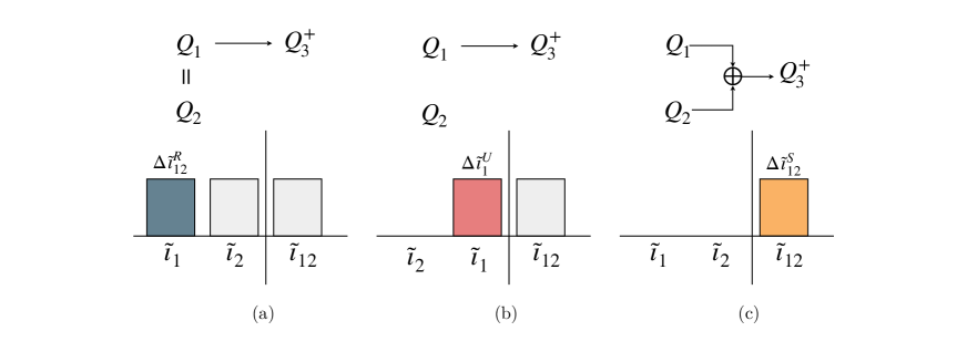
Figure 5: Schematic of simple examples (top panels) and associated specific mutual information (bottom panels) for (a) duplicated input (pure redundant causality), (b) output equal to first input (pure unique causality), and (c) exclusive-OR output (pure synergistic causality). The schematics of the specific mutual information apply to both states $Q_{3}^{+}=0$ and $Q_{3}^{+}=1$.

2.4 Contribution of different intensities to IT-causality

The IT-causalities can be decomposed in terms of different contributions from $\boldsymbol{Q}_{\boldsymbol{i}}$ and $Q_{j}^{+}$. For the case of the unique causality, the IT-causality as function of $q_{i}$ and $q_{j}^{+}$ is denoted by $\Delta\zeta^{U}_{i\rightarrow j}$ and it is such that

$$\Delta I^{U}_{i\rightarrow j}=\sum_{q_{i}}\sum_{q^{+}_{j}}\Delta\zeta^{U}_{i\rightarrow j}(q_{i},q_{j}^{+}).$$ (15)

The expression for $\Delta\zeta^{U}_{i\rightarrow j}$ is obtained inverting Eq. (15)

$$\Delta\zeta^{U}_{i\rightarrow j}=\begin{cases}p(q^{+}_{j})p(q_{i}|q^{+}_{j})\log_{2}\left(\frac{p(q^{+}_{j}|q_{i})}{p(q^{+}_{j})}\right)-p(q^{+}_{j})\frac{\tilde{\imath}_{l}}{N_{Q}},&\text{for}\ \tilde{\imath}_{i}\geq\tilde{\imath}_{l},\\ 0,&\text{otherwise},\end{cases}$$ (16)

where $\tilde{\imath}_{l}$ is the second largest member in $\tilde{\mathcal{G}}^{1}$ and $N_{Q}$ is the total number of states of $q_{i}$.

Analogous definitions can be written for the redundant and synergistic causalities. Note that $\Delta\zeta^{U}_{i\rightarrow j}$ may be negative for a given $q_{i}$–$q_{j}^{+}$ pair; although the sum of all the components is non-negative. Positive values of $\Delta\zeta^{U}_{i\rightarrow j}$ are informative (the pair $q_{i}$–$q_{j}^{+}$ occurs more frequently than would be expected) and negative values are misinformative (the pair $q_{i}$–$q_{j}^{+}$ occurs less frequently than would be expected).

2.5 Properties of IT-causality

We discuss some properties of the IT-causality.

• Non-negativity. All the terms in Eq. (9) are non-negative by the definition of the redundant, unique and synergistic causalities, and the non-negativity of the specific mutual information (DeWeese & Meister, 1999).

• Reconstruction of individual mutual information. The mutual information between $Q_{i}$ and $Q_{j}^{+}$ is equal to the unique and redundant causalities containing $Q_{i}$

  $$I(Q_{i};Q_{j}^{+})=\Delta I_{i\rightarrow j}^{U}+\sum_{\boldsymbol{i}\in\mathcal{C}_{i}}\Delta I_{\boldsymbol{i}\rightarrow j}^{R},$$ (17)

  where $\mathcal{C}_{i}$ is the set of the combinations in $\mathcal{C}$ containing the variable $Q_{i}$. This condition aligns with the notion that the information shared between $Q_{i}$ and $Q_{j}^{+}$ comprises contributions from unique and redundant information. However, there is no contribution from synergistic information, as the latter only arises through the combined effects of variables. This property, along with the non-negativity and forward propagation of information, enables the construction of the causality diagrams as depicted in figure 6 for two and three variables.

  (a)

  (b)

  Figure 6: Diagram of the decomposition into redundant, unique, and synergistic causalities and contributions to total and individual mutual information for (a) two variables and (b) three variables.

• Zero-causality property. If $Q_{j}^{+}$ is independent of $Q_{i}$, then $\Delta I^{R}_{\boldsymbol{i}\rightarrow j}=0$ for $\boldsymbol{i}\in\mathcal{C}_{i}$ and $\Delta I^{U}_{i\rightarrow j}=0$ as long as $Q_{i}$ is observable.

• Invariance under invertible transformations. The redundant, unique, and synergistic causalities are invariant under invertible transformations of $\boldsymbol{Q}$. This property follows from the invariance of the mutual information (Cover & Thomas, 2006).

3 Validation in stochastic systems

We discuss four illustrative examples highlighting key distinctions between IT-causality and time cross-correlations. These examples are not representative of any specific dynamical system. However, the phenomena they portray are expected to emerge to varying degrees in more complex systems. For comparisons, the “causality” based on the time cross-correlation from $Q_{i}$ to $Q_{j}$ is defined as

$$C_{i\rightarrow j}=\frac{|\sum_{n=1}^{N_{t}}Q_{i}^{\prime}(t_{n})Q_{j}^{\prime}(t_{n}+\Delta T)|}{\left(\sum_{n=1}^{N_{t}}Q_{i}^{\prime 2}(t_{n})\right)^{1/2}\left(\sum_{n=1}^{N_{t}}Q_{j}^{\prime 2}(t_{n})\right)^{1/2}}\geq 0,$$ (18)

where $Q_{i}^{\prime}(t_{n})$ signifies the fluctuating component of $Q_{i}(t_{n})$ at time $t_{n}$ with respect to its mean value, and $N_{t}$ is the total number of time steps considered for the analysis. The values of Eq. (18) are bounded between 0 and 1.

In all the scenarios discussed below, we consider a system with three variables $Q_{1}(t_{n})$, $Q_{2}(t_{n})$, and $Q_{3}(t_{n})$ with discrete times $t_{n}=n$. The systems is initialized at the first step with $Q_{1}(1)=Q_{2}(1)=Q_{3}(1)=0$. A time-varying stochastic forcing, denoted by $W_{i}(t_{n})$, acts on $Q_{i}(t_{n})$ following a Gaussian distribution with a mean of zero and standard deviation of one. IT-causality is computed for the time lag $\Delta T=1$ using a partition of 50 uniform bins per variable. The integration of the systems is carried out over $10^{8}$ time steps and the first 10,000 steps are excluded from the analysis to avoid transient effects.

• Mediator variable ($Q_{3}\rightarrow Q_{2}\rightarrow Q_{1}$). The first example corresponds to the system:

  $$Q_{1}(n+1) =\sin[Q_{2}(n)]+0.01W_{1}(n),$$ (19a)

  $$Q_{2}(n+1) =\cos[Q_{3}(n)]+0.01W_{2}(n),$$ (19b)

  $$Q_{3}(n+1) =0.9Q_{3}(n)+0.1W_{3}(n),$$ (19c)

  where $Q_{2}$ is the mediator variable between $Q_{1}$ and $Q_{3}$. The results are shown in figure 7, which includes an schematic of the functional dependence among variables, the IT-causality, and time cross-correlations. IT-causality reveals the prevalence of the unique contributions $\Delta I^{U}_{3\rightarrow 3}$, $\Delta I^{U}_{3\rightarrow 2}$, and $\Delta I^{U}_{2\rightarrow 1}$, in addition to some redundant contributions consistent with figure 7(a). The unique causalities are compatible with the functional dependency $Q_{3}\rightarrow Q_{2}\rightarrow Q_{1}$. This is less evident when using correlations, as $C_{1\rightarrow 1}$, $C_{2\rightarrow 1}$, $C_{1\rightarrow 2}$, and $C_{2\rightarrow 2}$ are large with values between 0.5 and 0.95. IT-causality also provides information about the amount of information leak (i.e. missing causality), which is above 50% for all three variables due to the effect of the stochastic forcing terms (which assumed to be unknown). The latter cannot be quantified using correlations.

  (a)

  

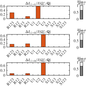
  (b)

  

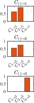
  (c)

  Figure 7: System with mediator variable from Eq. (19). (a) Schematic of the functional dependence among variables. $W_{i}$ represents stochastic forcing to the variable. (b) Redundant, unique and synergistic causalities. The grey bar is the information leak. The IT-causalities are ordered from left to right according to $N_{\boldsymbol{i}\rightarrow j}^{\alpha}$. (c) Time cross-correlation between variables.

• Confounder variable ($Q_{3}\rightarrow Q_{1}$ and $Q_{3}\rightarrow Q_{2}$). The second example considered is:

  $$Q_{1}(n+1) =\sin[Q_{1}(n)+Q_{3}(n)]+0.01W_{1}(n),$$ (20a)

  $$Q_{2}(n+1) =\cos[Q_{2}(n)-Q_{3}(n)]+0.01W_{2}(n),$$ (20b)

  $$Q_{3}(n+1) =0.9Q_{3}(n)+0.1W_{3}(n),$$ (20c)

  where $Q_{3}$ is a confounder variable to $Q_{1}$ and $Q_{2}$. The results are depicted in figure 8. The influence of the confounder variable becomes apparent through the synergistic causalities, namely, $\Delta I^{S}_{13\rightarrow 1}$ and $\Delta I^{S}_{23\rightarrow 2}$, as $Q_{3}$ co-occurs with $Q_{1}$ and $Q_{2}$ in Eq. (20a) and Eq. (20b), respectively. The unique causality $\Delta I^{U}_{3\rightarrow 3}$ dominates $Q_{3}$. The non-zero redundant causality $\Delta I^{R}_{123\rightarrow 3}$ implies that all variables contain information about the future of $Q_{3}$, but that information is already contained in the past of $Q_{3}$. When considering correlations, drawing robust conclusions regarding the interplay among variables presents a greater challenge due to the strong correlations observed across all possible pairs of variables, with values ranging between 0.6 and 1.

  (a)

  

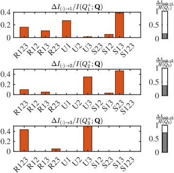
  (b)

  

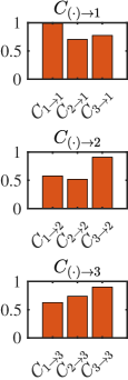
  (c)

  Figure 8: System with a confounder variable from Eq. (20). (a) Schematic of the functional dependence among variables. $W_{i}$ represents stochastic forcing to the variable. (b) Redundant, unique and synergistic causalities. The grey bar is the information leak. The IT-causalities are ordered from left to right according to $N_{\boldsymbol{i}\rightarrow j}^{\alpha}$. (c) Time cross-correlation between variables.

• Collider with synergistic variables ($[Q_{2},Q_{3}]\rightarrow Q_{1}$). The third example correspond to the system:

  $$Q_{1}(n+1) =\sin[Q_{2}(n)Q_{3}(n)]+0.001W_{1}(n),$$ (21a)

  $$Q_{2}(n+1) =0.9Q_{2}(n)+0.1W_{2}(n),$$ (21b)

  $$Q_{3}(n+1) =0.9Q_{3}(n)+0.1W_{3}(n),$$ (21c)

  where $Q_{2}$ and $Q_{3}$ work synergistically to influence $Q_{1}$. Essentially, $Q_{2}Q_{3}$ behaves as a single random variable acting on $Q_{1}$. The results, depicted in figure 9, clearly reveal the synergistic effect of $Q_{2}$ and $Q_{3}$ on $Q_{1}$, as evidenced by $\Delta I^{S}_{23\rightarrow 1}$. It is worth noting that, in this case, correlations do not hint at any influence of $Q_{2}$ and $Q_{3}$ on $Q_{1}$.

  (a)

  

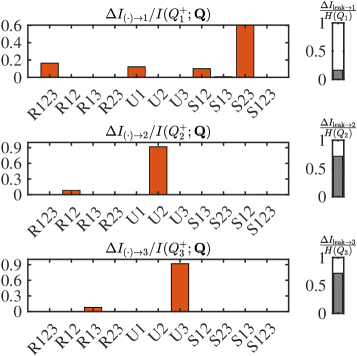
  (b)

  

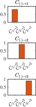
  (c)

  Figure 9: Collider with synergistic variables from Eq. (21). (a) Schematic of the functional dependence among variables. $W_{i}$ represents stochastic forcing to the variable. (b) Redundant, unique and synergistic causalities. The grey bar is the information leak. The IT-causalities are ordered from left to right according to $N_{\boldsymbol{i}\rightarrow j}^{\alpha}$. (c) Time cross-correlation between variables.

  (a)

  

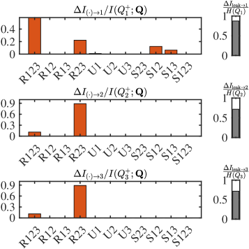
  (b)

  

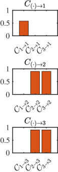
  (c)

  Figure 10: Collider with redundant variables from Eq. (22). (a) Schematic of the functional dependence among variables. $W_{i}$ represents stochastic forcing to the variable. (b) Redundant, unique and synergistic causalities. The grey bar is the information leak. The IT-causalities are ordered from left to right according to $N_{\boldsymbol{i}\rightarrow j}^{\alpha}$. (c) Time cross-correlation between variables.

• Collider with redundant variables ($Q_{2}\equiv Q_{3}\rightarrow Q_{1}$). The last example corresponds to the system:

  $$Q_{1}(n+1) =0.3Q_{1}(n)+0.7\{\sin[Q_{2}(n)Q_{3}(n)]+0.1W_{1}(n)\}$$ (22a)

  $$Q_{2}(n+1) =0.9Q_{2}(n)+0.1W_{2}(n),$$ (22b)

  $$Q_{3}(n+1) \equiv Q_{2}(n+1),$$ (22c)

  where $Q_{3}$ is identical to $Q_{2}$. In this scenario, both $Q_{2}$ and $Q_{3}$ convey the same information regarding each other influence on the future of $Q_{1}$. Consistently, the non-zero IT-causalities for $Q_{2}$ and $Q_{3}$ are $\Delta I^{R}_{23\rightarrow 2}=\Delta I^{R}_{23\rightarrow 3}\neq 0$. The active IT-causalities in $Q_{1}$ is the redundant contribution $\Delta I^{R}_{123\rightarrow 1}$ and $\Delta I^{R}_{23\rightarrow 1}$. The variables $Q_{2}$ and $Q_{3}$ are also highly correlated, but no assessment can be made about their redundancy from the correlation viewpoint. Furthermore, the correlation analysis do not show any influence from $Q_{2}$ and $Q_{3}$ to $Q_{1}$.

Additional validation cases are offered in the Appendix B. These include coupled logistic maps with synchronization and coupled Rössler-Lorenz system.

4 Scale locality of the energy cascade in isotropic turbulence

The cascade of energy in turbulent flows, namely, the transfer of kinetic energy from large to small flow scales or vice versa (backward cascade), has been the cornerstone of most theories and models of turbulence since the 1940s  (e.g., Richardson, 1922; Obukhov, 1941; Kolmogorov, 1941, 1962; Aoyama et al., 2005; Falkovich, 2009; Cardesa et al., 2017). However, understanding the dynamics of kinetic energy transfer across scales remains an outstanding challenge. Given the ubiquity of turbulence, a deeper understanding of the energy transfer among the flow scales could enable significant progress across various fields, ranging from combustion  (Veynante & Vervisch, 2002), meteorology  (Bodenschatz, 2015), and astrophysics  (Young & Read, 2017) to engineering applications of aero/hydrodynamics  (Sirovich & Karlsson, 1997; Hof et al., 2010; Marusic et al., 2010; Kühnen et al., 2018; Ballouz & Ouellette, 2018). Despite the progress made in recent decades, the causal interactions of energy among scales in the turbulent cascade have received less attention. Here, we investigate the redundant, unique, and synergistic causality of turbulent kinetic energy transfer across different scales. The primary hypothesis under consideration here is the concept of scale locality within the cascade, where kinetic energy is transferred sequentially from one scale to the subsequent smaller scale.

4.1 Numerical database

The case chosen to study the energy cascade is forced isotropic turbulence in a triply periodic box with side $L$. The data were obtained from the DNS of Cardesa et al. (2015), which is publicly available in Torroja (2021). The conservation of mass and momentum equations of an incompressible flow are given by

$$\frac{\partial u_{i}}{\partial t}+\frac{\partial u_{i}u_{j}}{\partial x_{j}}=-\frac{\partial\Pi}{\partial x_{i}}+\nu\frac{\partial^{2}u_{i}}{\partial x_{j}\partial x_{j}}+f_{i},\quad\frac{\partial u_{i}}{\partial x_{i}}=0,$$ (23)

where repeated indices imply summation, $\boldsymbol{x}=[x_{1},x_{2},x_{3}]$ are the spatial coordinates, $u_{i}$ for $i=1,2,3$ are the velocities components, $\Pi$ is the pressure, $\nu$ is the kinematic viscosity, and $f_{i}$ is a linear forcing sustaining the turbulent flow (Rosales & Meneveau, 2005). The flow setup is characterized by Reynolds number based on the Taylor microscale (Pope, 2000), $Re_{\lambda}\approx 380$. The simulation was conducted by direct numerical simulation of Eq. (23) with $1024^{3}$ spatial Fourier modes, which is enough to accurately resolve all the relevant length-scales of the flow.

In the following, we provide a summary of the main parameters of the simulation. For more detailed information about the flow setup, the readers are referred to Cardesa et al. (2015). The spatial and time-averaged values of turbulent kinetic energy ($K=u_{i}u_{i}/2$) and dissipation ($\varepsilon=2\nu S_{ij}S_{ij}$) are indicated as $K_{\mathrm{avg}}$ and $\varepsilon_{\mathrm{avg}}$, respectively. Here, $S_{ij}=(\partial u_{i}/\partial x_{j}+\partial u_{j}/\partial x_{i})/2$ represents the rate-of-strain tensor. The ratio between the largest and smallest length scales in the problem can be quantified as $L_{\varepsilon}/\eta=1800$, where $L_{\varepsilon}=K_{\mathrm{avg}}^{3/2}/\varepsilon_{\mathrm{avg}}$ denotes the integral length scale, and $\eta=(\nu^{3}/\varepsilon_{\mathrm{avg}})^{1/4}$ signifies the Kolmogorov length scale. The generated data is also time-resolved, with flow fields being stored at intervals of $\Delta t=0.0076T_{\varepsilon}$, where $T_{\varepsilon}=K_{\mathrm{avg}}/\varepsilon_{\mathrm{avg}}$. The simulation was intentionally run for an extended period to ensure the accurate computation of specific mutual information. The total simulated time after transient effects was equal to $165T_{\varepsilon}$.

4.2 Characterization of the kinetic energy transfer

The next stage involves quantifying the transfer of kinetic energy among eddies at different length scales over time. To accomplish this, the $i$-th component of the instantaneous flow velocity, denoted as $u_{i}(\boldsymbol{x},t)$, is decomposed into contributions from large and small scales according to $u_{i}(\boldsymbol{x},t)=\bar{u}_{i}(\boldsymbol{x},t)+u^{\prime}_{i}(\boldsymbol{x},t)$. The operator $\bar{(\cdot)}$ signifies the low-pass Gaussian filter given by

$$\bar{u}_{i}(\boldsymbol{x},t)=\iiint_{V}\frac{\sqrt{\pi}}{\bar{\Delta}}\exp\left[-\pi^{2}(\boldsymbol{x}-\boldsymbol{x}^{\prime})^{2}/\bar{\Delta}^{2}\right]u_{i}(\boldsymbol{x}^{\prime},t)\mathrm{d}\boldsymbol{x}^{\prime},$$ (24)

where $\bar{\Delta}$ is the filter width and $V$ denotes integration over the whole flow domain. Examples of the unfiltered and filtered velocities are included in figure 11.

(a)

(b)

Figure 11: Instantaneous velocity field for (a) $u_{1}$ and (b) $\bar{u}_{1}$. The velocities are normalized by their respective standard deviations.

The kinetic energy of the large-scale field evolves as

$$\left(\frac{\partial}{\partial t}+\bar{u}_{j}\frac{\partial}{\partial x_{j}}\right)\frac{1}{2}\bar{u}_{i}\bar{u}_{i}=-\frac{\partial}{\partial x_{j}}\left(\bar{u}_{j}\bar{\Pi}+\bar{u}_{i}\tau_{ij}-2\nu\bar{u}_{i}\bar{S}_{ij}\right)+\Sigma-2\nu\bar{S}_{ij}\bar{S}_{ij}+\bar{u}_{i}\bar{f}_{i},$$ (25)

where $\tau_{ij}=(\overline{u_{i}u_{j}}-\bar{u}_{i}\bar{u}_{j})$ is the subgrid-scale stress tensor, which represents the effect of the (filtered) small-scale eddies on the (resolved) large-scale eddies. The interscale energy transfer between the filtered and unfiltered scales is given by

$$\Sigma(\boldsymbol{x},t;\bar{\Delta})=\tau_{ij}(\boldsymbol{x},t;\bar{\Delta}_{i})\bar{S}_{ij}(\boldsymbol{x},t;\bar{\Delta}_{i}),$$ (26)

which is the quantity of interest.

The velocity field is low-pass filtered at four filter widths: $\bar{\Delta}_{1}=163\eta$, $\bar{\Delta}_{2}=81\eta$, $\bar{\Delta}_{3}=42\eta$, and $\bar{\Delta}_{4}=21\eta$. The filter widths are situated within the inertial range of the simulation: $L_{\varepsilon}>\bar{\Delta}_{i}>\eta$, for $i=1,2,3$ and 4. The resulting velocity fields are used to compute the interscale energy transfer at scale $\bar{\Delta}_{i}$, which is denoted by $\Sigma_{i}(\boldsymbol{x},t;\bar{\Delta}_{i})$. We use the volume-averaged value of $\Sigma_{i}$ computed over the entire domain, denoted by $\langle\Sigma_{i}\rangle$, as a marker for the time-evolution of the interscale energy transfer:

$$\langle\Sigma_{i}\rangle(t)=\iiint_{V}\Sigma(\boldsymbol{x},t;\bar{\Delta}_{i})\mathrm{d}\boldsymbol{x},$$ (27)

which is only a function of time for a given $\bar{\Delta}_{i}$. Figure 12(a) contains a fragment of the time history of $\langle\Sigma_{i}\rangle$ for $i=1,2,3$ and $4$.

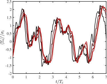
(a)

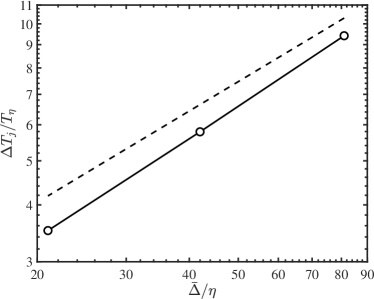
(b)

Figure 12: (a) Extract of the time-history of fluctuating component of $\langle\Sigma_{1}\rangle$, $\langle\Sigma_{2}\rangle$, $\langle\Sigma_{3}\rangle$, and $\langle\Sigma_{4}\rangle$ (from black to red). Although not shown, the whole time-span of the signals is $165T_{\varepsilon}$. The primes denote fluctuating component above the mean value and $\sigma_{i}$ is the standard deviation of $\langle\Sigma_{i}\rangle$. (b) Time horizon of causal influence for maximum unique causuality from $\langle\Sigma_{i}\rangle$ to $\langle\Sigma_{j}\rangle^{+}$. $\Delta I^{U}_{i\rightarrow j}$ with $j\neq i$ as a function of the filter width. The dashed line is $\Delta T_{j}\sim\bar{\Delta}^{2/3}$. $T_{\eta}$ and $\eta$ are the Kolmorogov time-scale and length-scale, respectively.

4.3 IT-causality analysis of the energy cascade

We examine the causal interactions among the variables representing the interscale turbulent kinetic energy transfer: $\langle\mathbf{\Sigma}\rangle=[\langle\Sigma_{1}\rangle,\langle\Sigma_{2}\rangle,\langle\Sigma_{3}\rangle,\langle\Sigma_{4}\rangle]$. For a given target variable, $\langle\Sigma_{j}\rangle$, the time delay $\Delta T_{j}$ used to evaluate causality is determined as the time required for maximum $\Delta I^{U}_{i\rightarrow j}$ with $j\neq i$, where $\langle\Sigma_{j}\rangle^{+}$ is evaluated at $t+\Delta T_{j}$. Figure 12(b) shows that the time lags for causal influence increase with the filter width. According to the Kolmogorov theory (Kolmogorov, 1941), the characteristic lifetime of an eddy in the inertial range scales as $\sim\bar{\Delta}^{2/3}$. Assuming that the time required for interscale energy transfer is proportional to the eddy lifetime, it is expected that $\Delta T_{j}\sim\bar{\Delta}^{2/3}$. The values of $\Delta T_{j}$ are consistent with the scaling provided by $\bar{\Delta}^{2/3}$ (also included in the figure), albeit the observation is limited to only three scales due to low Reynolds number effects. It was tested that the conclusions drawn below are not affected when the value of $\Delta T_{j}$ was halved and doubled.

The redundant, unique, and synergistic causalities are shown in figure 13(a) for each $\langle\Sigma_{j}\rangle$, $j=1,\ldots,4$. The most important contributions come from redundant and unique causalities, whereas synergistic causalities play a minor role. The top panel in figure 13(b) shows the causal map for $\Delta I^{U}_{i\rightarrow j}$. It is interesting that the causal map for unique causalities vividly captures the forward energy cascade of causality toward smaller scales, which is inferred from the non-zero terms $\Delta I^{U}_{1\rightarrow 2}$, $\Delta I^{U}_{2\rightarrow 3}$, and $\Delta I^{U}_{3\rightarrow 4}$. Curiously, there is no unique causality observed from smaller to larger scales, and any backward causality solely arises through redundant causal relationships. In the context of IT-causality, this implies that no new information is conveyed from the smaller scales to the larger ones.

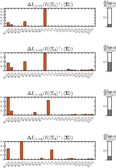
(a)

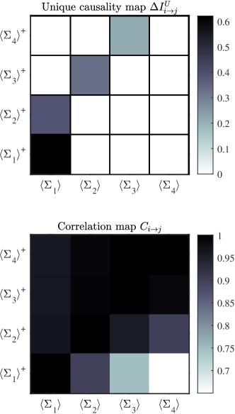
(b)

Figure 13: (a) Redundant (R), unique (U), and synergistic (S) causalities among interscale energy-transfer signals at different scales. The information leak for each variable is also shown in the right-hand side bar. The causalities are ordered from left to right according to $N_{\boldsymbol{i}\rightarrow j}^{\alpha}$. (b) Top panel: causality maps for unique causalities $\Delta I^{U}_{i\rightarrow j}$. Bottom panel: Correlation map $C_{i\rightarrow j}$ between interscale energy-transfer signals as defined by Eq. (18).

It is also revealing to compare the results in the top panel of figure 13(b) with the time cross-correlation, as the latter is routinely employed for causal inference by the fluid mechanics community. The time-cross-correlation “causality” from $\langle\Sigma_{i}\rangle$ to $\langle\Sigma_{j}\rangle$ is defined using Eq. (18) with $Q_{i}=\langle\Sigma_{i}\rangle$ and $Q_{j}=\langle\Sigma_{j}\rangle$. The time lag $\Delta T_{ij}$ depends on the pair $\langle\Sigma_{i}\rangle$–$\langle\Sigma_{j}\rangle$ and is obtained as the time for maximum correlation. The correlation map, $C_{i\rightarrow j}$, is shown in the bottom panel of figure 13(b). The process portrayed by $C_{i\rightarrow j}$ is far more intertwined than its IT-causality counterpart offered in the top panel of figure 13(b). Similarly to $\Delta I^{U}_{i\rightarrow j}$, the correlation map also reveals the prevailing nature of the forward energy cascade ($C_{i\rightarrow j}$ larger for $j>i$). However, note that $C_{i\rightarrow j}$ is always above 0.7, implying that all the interscale energy transfers are tightly coupled. This is due to the inability of $C_{i\rightarrow j}$ to compensate for mediator variables (e.g., a cascading process of the form $\langle\Sigma_{1}\rangle\rightarrow\langle\Sigma_{2}\rangle\rightarrow\langle\Sigma_{3}\rangle$ would result in a non-zero correlation between $\langle\Sigma_{1}\rangle$ and $\langle\Sigma_{3}\rangle$ via the mediator variable $\langle\Sigma_{2}\rangle$). As a consequence, $C_{i\rightarrow j}$ also fails to shed light on whether the energy is cascading locally from the large scales to the small scales (i.e., $\langle\Sigma_{1}\rangle\rightarrow\langle\Sigma_{2}\rangle\rightarrow\langle\Sigma_{3}\rangle\rightarrow\langle\Sigma_{4}\rangle$), or on the other hand, the energy is transferred between non-contiguous scales (e.g., $\langle\Sigma_{1}\rangle\rightarrow\langle\Sigma_{3}\rangle$ without passing through $\langle\Sigma_{2}\rangle$). We have seen that IT-causality supports the former: the energy is transferred sequentially.

Overall, the inference of causality based on the time cross-correlation is obscured by the often milder asymmetries in $C_{i\rightarrow j}$ and the failure of $C_{i\rightarrow j}$ to account for the effects of intermediate variables. In contrast, the causal map of unique causalities $\Delta I^{U}_{i\rightarrow j}$ conveys a more intelligible picture of the locality of energy transfers among different scales. Our conclusions are consistent with evidence from diverse approaches, such as scaling analysis (Zhou, 1993a, b; Eyink, 1995; Aoyama et al., 2005; Eyink, 2005; Mininni et al., 2006, 2008; Aluie & Eyink, 2009; Eyink & Aluie, 2009), triadic interactions in Fourier space (Domaradzki & Rogallo, 1990; Domaradzki et al., 2009), time cross-correlations (Cardesa et al., 2015, 2017), and transfer entropy in the Gledzer–Ohkitana–Yamada shell model (Materassi et al., 2014).

The IT-causality can be decomposed into contributions from different intensities of the target variable ($\langle\Sigma_{j}\rangle^{+}$). This information is provided by the weighted specific causalities $p(\langle\Sigma_{j}\rangle^{+})\Delta\tilde{\imath}_{\alpha\rightarrow j}^{\alpha}$, which are shown in figure 14(a) for $\langle\Sigma_{2}\rangle^{+}$. The unique causalities can also be decomposed as a function of the source variable. This is done for the unique causality from $\langle\Sigma_{1}\rangle$ to $\langle\Sigma_{2}\rangle^{+}$, denoted by $\Delta\zeta^{U}_{1\rightarrow 2}$ (as seen in figure 14b). The results show that the unique causality follows the linear relationship $\langle\Sigma_{1}\rangle^{\prime}\sim{\langle\Sigma_{2}\rangle^{\prime}}^{+}$. In general, events located around the mean value contribute the most to the causality. However, there is a small bias towards values above the mean $\langle\Sigma_{1}\rangle^{\prime}>0$. Similar conclusions can be drawn for the other unique causalities (not shown).

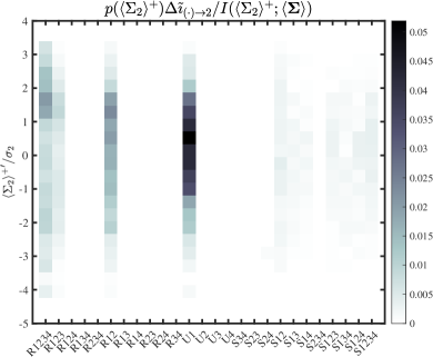
(a)

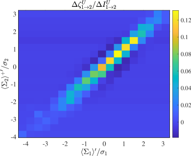
(b)

Figure 14: Specific (a) Redundant (R), unique (U), and synergistic (S) causalities from $\langle\Sigma_{i}\rangle$ to $\langle\Sigma_{2}\rangle^{+}$ as a function of the intensity of $\langle\Sigma_{2}\rangle^{+}$. (b) Decomposition of unique causality as a function of $\langle\Sigma_{1}\rangle$ and $\langle\Sigma_{2}\rangle^{+}$. The primes denote fluctuating component above the mean value and $\sigma_{i}$ is the standard deviation of $\langle\Sigma_{i}\rangle$.

Finally, we calculate the information leak ($\Delta I_{\mathrm{leak}\rightarrow j}$) to quantify the amount of causality unaccounted for by the observable variables. The ratios $\Delta I_{\mathrm{leak}\rightarrow j}/H(\langle\Sigma_{j}\rangle)$ are found to be 0.14, 0.47, 0.31, and 0.20 for $j=1,2,3$, and 4, respectively, and for the time lags considered. The largest leak occurs for $\langle\Sigma_{2}\rangle$, where approximately 47% of the IT-causality is carried by variables not included within the set $[\langle\Sigma_{1}\rangle,\langle\Sigma_{2}\rangle,\langle\Sigma_{3}\rangle,\langle\Sigma_{4}\rangle]$. This implies that there are other factors affecting $\langle\Sigma_{2}\rangle$ that have not been accounted for and that explain the remaining 53% causality of the variable. Conversely, the largest scale $\langle\Sigma_{1}\rangle$ bears the smallest leak of 14%, which is due to the high value of the unique causality $\Delta I^{U}_{1\rightarrow 1}$. The latter implies that the future of $\langle\Sigma_{1}\rangle$ is mostly determined by its own past.

5 Interaction between inner and outer layer motions in wall-bounded turbulence

The behavior of turbulent motion within the thin fluid layers immediately adjacent to solid boundaries poses a significant challenge for understanding and prediction. These layers are responsible for nearly 50% of the aerodynamic drag on modern airliners and play a crucial role in the first 100 meters of the atmosphere, influencing broader meteorological phenomena (Marusic et al., 2010). The physics in these layers involve critical processes occurring very close to the solid boundary, making accurate measurements and simulations exceptionally difficult.

Previous investigations utilizing experimental data from high Reynolds number turbulent boundary layers have revealed the impact of large-scale boundary-layer motions on the smaller-scale near-wall cycle (e.g. Hutchins & Marusic, 2007; Mathis et al., 2009). To date, the consensus holds that the dynamics of the near-wall layer operate autonomously (Jiménez & Pinelli, 1999), implying that outer-scale motions are not necessary to sustain a realistic turbulence in the buffer layer. Similarly, the large-scale outer-layer flow motions are known to be insensitive to perturbations of the near-wall cycle (Townsend, 1976). Nevertheless, it is widely accepted that the influence of large-scale motions in the inner layer is manifested through amplitude modulation of near-wall events.

In the initial studies aimed at understanding outer-inner layer interactions (Mathis et al., 2009; Marusic et al., 2010; Mathis et al., 2011; Agostini & Leschziner, 2014), temporal or spatial signals of large-scale streamwise velocity motions were extracted using pre-defined filter cut-offs. The superposition of the large- and small-scale fluctuations in the near-wall region was then parameterized assuming universal small-scale fluctuations in the absence of inner–outer interactions. Subsequent refinements of the method include the work by Agostini & Leschziner (2016), who separated the large-scale and small-scale motions by means of the Empirical Mode Decomposition (Huang et al., 1998; Cheng et al., 2019) without explicit wavelength cutoffs. Later, Agostini & Leschziner (2022) used an auto-encoder algorithm to separate three-dimensional flow fields into large-scale and small-scale motions. Recently, Towne et al. (2023) used conditional transfer entropy to study inner/outer layer interactions in a turbulent boundary layer. Howland & Yang (2018) also investigated the small-scale response to large-scale fluctuations in turbulent flows in a more general setting along with its implications on wall modeling. A discussion of the amplitude modulation process in other turbulent flows can be found in Fiscaletti et al. (2015).

Here, we leverage IT-causality to investigate the interaction between motions in the outer and inner layers of wall-bounded turbulence. Figure 15 illustrates the configuration used to examine the causal interactions between velocity motions in the outer layer and the inner layer. Two hypotheses are considered: (i) the footprint of outer flow large-scale motions on the near-wall motions and (ii) Townsend’s outer-layer similarity hypothesis (Townsend, 1976). In hypothesis (i), the dynamics of the near-wall motions are presumed to be influenced by outer flow large-scale motions penetration close to the wall (i.e., predominance of top-down causality). In hypothesis (ii), the outer region of a turbulent boundary layer is expected to exhibit universal behavior that is independent of the specific characteristics of the underlying wall surface (i.e., lack of bottom-up causality).

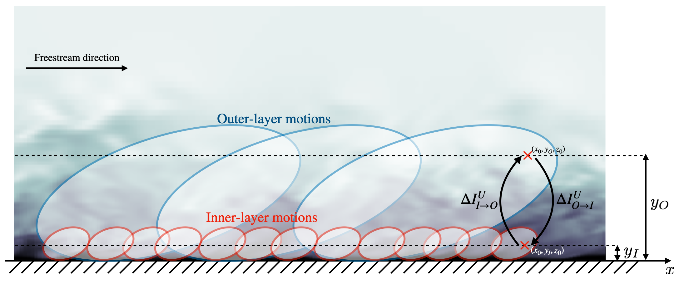
Figure 15: Schematic of outer-layer and inner-layer streamwise velocity motions in a turbulent boundary and their interactions via unique causality.

5.1 Numerical database

The database utilized is a turbulent channel flow at friction Reynolds number Re${}_{\tau}=u_{\tau}h/\nu\approx 1,000$ from Lozano-Durán & Jiménez (2014) based on the channel half-height ($h$), the kinematic viscosity ($\nu$), and the average friction velocity at the wall ($u_{\tau}$). The simulation was generated by solving the incompressible Navier–Stokes equations between two parallel walls via direct numerical simulation. The size of the domain in the streamwise, wall-normal, and spanwise direction is $2\pi h\times 2h\times\pi h$, respectively. Velocity fields were stored sequentially in time every 0.8 plus units to resolve a large amount of the frequency content of the turbulent flow. Here, plus units are defined in terms of the friction velocity and the kinematic viscosity. The streamwise, wall-normal, and spanwise directions of the flow are denoted by $x$, $y$, and $z$, respectively. More details about the simulation set-up can be found in Lozano-Durán & Jiménez (2014).

The time-resolved signals considered are those of the streamwise velocity at the wall-normal heights $y_{I}^{*}=15$ (for the inner layer) and $y_{O}/h=0.3$ (for the outer layer), where superscript $*$ denotes plus units. The inner and outer layer streamwise velocity signals are denoted by $u_{I}(t)=u(x,y_{I},z,t)$ and $u_{O}(t)=u(x,y_{O},z,t)$, respectively. Figure 16 shows an excerpt of $u_{I}$ and $u_{O}$ for a fixed $(x,z)$ location. The joint probability distribution to evaluate IT-causality was calculated using multiple streamwise and spanwise locations $(x,z)$. Some studies have considered a space-shift in the streamwise direction between both signals to increase their correlation (Howland & Yang, 2018). Here, we do not apply a streamwise space-shift between the two signals but instead we do account for the relative displacement between signals using the time lag $\Delta T$ to evaluate the IT-causality.

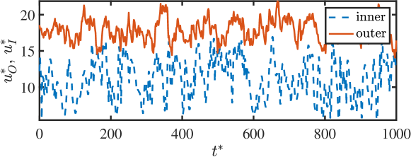
Figure 16: Example of time signals of the streamwise velocity in the inner layer $u_{I}(x,y_{I},z,t)$ at $y_{I}^{*}=15$ (dashed) and the outer layer $u_{O}(x,y_{O},z,t)$ at $y_{O}/h=0.3$ (solid) for a fixed $(x,z)$. The signals are extracted from a turbulent channel flow at $\mathrm{Re}_{\tau}\approx 1,000$. The asterisk denotes plus units.

5.2 IT-causality analysis of inner/outer layer interactions

The goal is to evaluate the cause-and-effect interactions between $u_{I}$ and $u_{O}$. Four causal interactions are investigated: the self-induced unique causality of the signals, $\Delta I^{U}_{O\rightarrow O}$ (outer$\rightarrow$outer) and $\Delta I^{U}_{I\rightarrow I}$ (inner$\rightarrow$inner), and the cross-induced unique causality between signals, $\Delta I^{U}_{I\rightarrow O}$ (inner$\rightarrow$outer) and $\Delta I^{U}_{O\rightarrow I}$ (outer$\rightarrow$inner). The latter represents the interaction between outer and inner layer motions.

The self- and cross- unique causalities are compiled in figure 17 as a function of the time lag $\Delta T$. The self-induced unique causalities $\Delta I^{U}_{O\rightarrow O}$ and $\Delta I^{U}_{I\rightarrow I}$ dominate for short time-scales. This is expected, as variables are mostly causal to themselves in the immediate future. Regarding inner/outer interactions, there is a clear peak at $\Delta T^{*}\approx 30$ from the outer motions to the inner motions as seen in $\Delta I^{U}_{O\rightarrow I}$. This peak is absent in the reverse direction $\Delta I^{U}_{I\rightarrow O}$, which is essentially zero at all time scales. The result distinctly supports the prevalence of top-down interactions: causality flows predominantly from the outer-layer large-scale motions to inner-layer small-scale motions. The outcome is consistent with the modulation of the near-wall scales by large-scale motions reported in previous investigations (e.g. Hutchins & Marusic, 2007; Mathis et al., 2009). The lack of bottom-up causality from the inner layer to the outer layer is also consistent with the Townsend’s outer-layer similarity hypothesis (Townsend, 1976) and previous observations in the literature (e.g. Flack et al., 2005; Flores & Jiménez, 2006; Busse & Sandham, 2012; Mizuno & Jiménez, 2013; Chung et al., 2014; Lozano-Durán & Bae, 2019).

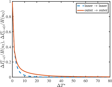
(a)

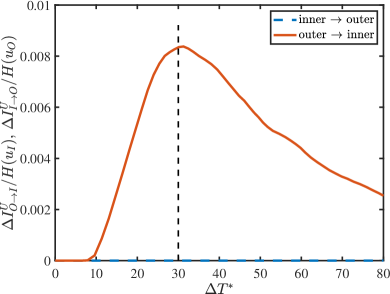
(b)

Figure 17: Unique causality of the inner and outer layer streamwise velocity motions. (a) Self- and (b) cross-induced unique causality as a function of the time lag. The vertical dashed line is $\Delta T^{*}=30$.

Figure 18(a) shows the redundant, unique, and synergistic causalities among velocity signals in the inner and outer layer at $\Delta T^{*}=30$. This value corresponds to the time lag of maximum causal inference for $\Delta I^{U}_{O\rightarrow I}$. The inner layer motions are dominated by the unique causality from the outer layer, $\Delta I^{U}_{O\rightarrow I}$. The redundant and synergistic causalities are lower but still significant. Curiously, the unique causality $\Delta I^{U}_{I\rightarrow I}$ is zero at the time scale considered. For the outer-layer motions, most of the causality is self-induced $\Delta I^{U}_{O\rightarrow O}$ with no apparent influence from the inner layer.

The information leak, as indicated in the right-hand sidebar, is 99% for both $u_{I}$ and $u_{O}$. Such a high value implies that most of the causality determining the future states of $u_{I}$ and $u_{O}$ is contained in other variables not considered in the analysis. This high information leak value is unsurprising, considering that the analysis has neglected most of the turbulent flow field to evaluate the causality of $u_{I}$ and $u_{O}$, retaining only the degrees of freedom represented by two pointwise signals.

The IT-causality is contrasted with the time cross-correlations in figure 18(b) using the same time lag of $\Delta T^{*}=30$. All correlations are below 30%. Nonetheless, the fact that $C_{O\rightarrow I}>C_{I\rightarrow O}$ also hints at the higher influence of the outer layer flow on the inner layer motions. However, this asymmetry in the directionality of the interactions is milder and less assertive than the IT-causality results. Furthermore, correlations do not offer a detailed decomposition into redundant, unique, and synergistic causality, nor do they account for the effect of unobserved variables as quantified by the information leak.

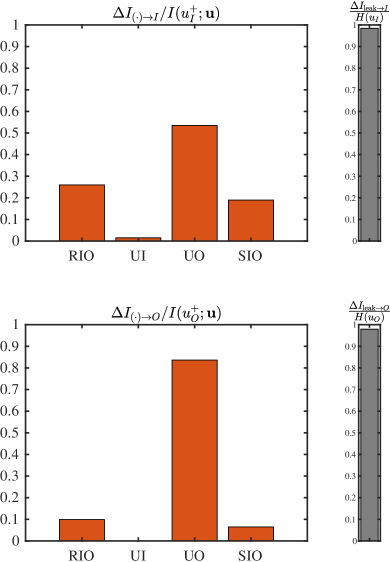
(a)

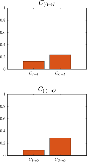
(b)

Figure 18: (a) Redundant (R), unique (U), and synergistic (S) causalities among velocity signals in the inner (I) and outer (O) layer of wall-bounded turbulence. The information leak for each variable is also shown in the right-hand side bar. (b) Time cross-correlation between variables. The results are for a time-lag $\Delta T^{*}\approx 30$.

Finally, we investigate the contribution of different intensities of $u_{O}$ and $u_{I}$ to the IT-causalities, focusing on top-down interactions. The redundant, unique, and synergistic specific causalities for $u_{I}^{+}$ are shown in figure 19(a). The unique causality as a function of $u_{O}$ and $u_{I}$ (namely, $\Delta\zeta^{U}_{O\rightarrow I}$) is presented in figure 19(b). The contributions are clearly divided into four quadrants. Most of the causality is located in the first quadrant ($u_{O}^{\prime}>0$ and $u_{I}^{\prime}>0$), followed by the third quadrant ($u_{O}^{\prime}<0$ and $u_{I}^{\prime}<0$), as both contain informative events ($\Delta\zeta^{U}_{O\rightarrow I}>0$). The second and fourth quadrants contain misinformative events ($\Delta\zeta^{U}_{O\rightarrow I}<0$) that do not increase the value of the unique causality. The results seem to indicate that causality from the outer to the inner layer primarily occurs within high-velocity streaks in the outer layer that propagate towards the wall. A significant, albeit weaker, causality is also observed for low-velocity streaks. It has been well-documented that high- and low-velocity streaks are statistically accompanied by downward and upward flow motions referred to as sweeps and ejections, respectively (Wallace, 2016), which explains the high values of $\Delta\zeta^{U}_{O\rightarrow I}$ for $u_{O}^{\prime}>0$-$u_{I}^{\prime}>0$ and $u_{O}^{\prime}<0$-$u_{I}^{\prime}<0$. The absence of causality for $u_{O}^{\prime}$ and $u_{I}^{\prime}$, with opposite signs, can be attributed to the fact that these situations are improbable, as they imply a change of sign in the velocity streak along the wall-normal direction.

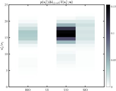
(a)

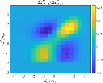
(b)

Figure 19: (a) Redundant (R), unique (U), and synergistic (S) specific causalities from $u_{O}$ to $u_{I}^{+}$ as a function of the intensity of $u_{I}^{+}$. (b) Decomposition of unique causality $\Delta\zeta^{U}_{O\rightarrow I}$ as a function of $u_{O}$ to $u_{I}^{+}$. The primes denote fluctuating component above the mean value and $\sigma_{u_{I}}$ and $\sigma_{u_{O}}$ are the standard deviations of $u_{O}$ to $u_{I}$, respectively.

In summary, in comparison to previous investigations, IT-causality is purposely devised to account for the time dynamics of the signals and provides the time scale for maximum causal inference. Moreover, the present approach only requires the inner/outer time signals without any further manipulation. IT-causality is based on probability distributions and, as such, is invariant under shifting, rescaling, and, in general, invertible transformations of the signals (see §2.5). Hence, our approach unveils the interactions between inner and outer layer velocity motions in a simple manner while minimizing the number of arbitrary parameters typically used in previous studies, such as the type of signal transformation, filter width, reference convection velocity, and selection of parameters for the extraction of the universal signal.

6 Limitations

We conclude this work by discussing several limitations of IT-causality for causal inference in chaotic dynamical systems:

• The first consideration is the acknowledgment that IT-causality is merely a tool. As such, it can offer valuable physical insights into the problem at hand when used effectively. The formulation of meaningful questions and the selection of appropriate variables to answer those questions will always take precedence over the choice of the tool.

• IT-causality operates within a probabilistic framework. The concept of information-theoretic causality used here is based on transitional probabilities between states. Therefore, it should be perceived as a probabilistic measure of causality rather than a means of quantifying causality for individual events or causality inferred from interventions into the system.

• IT-causality is a data-intensive tool due to the necessity of estimating high-dimensional probability distributions. Consequently, the applicability of the method is limited when dealing with a large number of variables. Typically, it can be applied to analyze up to five to ten variables simultaneously, depending on the available data. Attempting to consider a greater number of variables can introduce significant statistical errors. However, this limitation is expected to become less restrictive with the ongoing proliferation of data and advancements in probability estimation methods. Appendix C contains an analysis of the impact of the number of samples in IT-causality.

• IT-causality relies on mutual information, which is a specific instance of the Kullback-Leibler divergence. Other dissimilarity methods exist to quantify differences between probability distributions, all of which are equally valid and could be explored in the future to devise alternative quantification of causality.

• The results obtained through IT-causality analysis are contingent on the observable phase-space. High-dimensional chaotic systems, such as turbulence, involve nonlinear interactions among a large amount of variables. However, IT-causality is often limited to a finite subset of variables. When variables with a strong impact on the dynamics are unobserved or intentionally omitted due to practical constraints, the inferred causal structure among observed variables can be incomplete or misleading. This situation is referred to as lack of causal sufficiency. Appendix §B.2 contains an example of the impact of unobserved variables in the coupled Rössler-Lorenz system.

• The concept of causality, as interpreted in IT-causality, is inherently linked to changes in the variables. This is reflected in the partitioning of the variables into states ($D_{i}$), which are regions where variable values fall within a specific range. The partitioning scheme shapes our definition of change; a variable is considered to have changed when it transitions between states. Hence, different partitions may lead to different IT-causalities. For continuous variables, IT-causality will become eventually insensitive to further refinements of the partition provided the smoothness in the probability distributions, although exceptions may arise. Appendix C also provides an analysis of the sensitivity of IT-causality to partition refinement.

• IT-causality is specifically designed for dynamic variables and, as such, cannot be employed to analyze parameters that remain constant over time.

In summary, IT-causality may offer valuable insights into causality within complex systems, especially when compared to correlation-based methods. However, like any tool, it comes with constraints that researchers should be aware of when applying the approach to draw meaningful conclusions.

7 Conclusions

Causality lies at the heart of scientific inquiry, serving as the cornerstone for understanding how variables relate to one another. In the case of turbulence research, the chaotic and multiscale nature of the flow makes the quantification of causality particularly challenging. For that reason, traditional approaches for assessing relationships between variables often fall short in measuring causal links, highlighting the need for more in-depth approaches.

We have introduced an information-theoretic method to quantify causality among variables by measuring the dissimilarity between transitional probability distributions. The approach, referred to as IT-causality, is rooted in the forward propagation of information in chaotic dynamical systems and quantifies causality by measuring the information gained about future events. One distinctive feature of IT-causality compared to correlation-based methods is its suitability for analyzing causal networks that involve mediator, confounder, and collider variables. In the latter, our method allows us to distinguish between redundant, unique, and synergistic causality among variables. IT-causality can also be decomposed as a function of variable intensities, which facilitates the evaluation of how different states contribute to the overall causality. Another essential aspect of IT-causality is its foundation on probability distributions, rendering it invariant under shifting, rescaling, and general invertible transformations of the variables. Finally, we have introduced the concept of information leak, quantifying the extent of causality that remains unaccounted for due to unobserved variables.

IT-causality has been applied to investigate two problems in turbulence research. In the first problem, we tested the hypothesis of scale locality in the energy cascade of isotropic turbulence. Time-resolved data from direct numerical simulations of isotropic turbulence were used for the analysis. First, the velocity field was low-pass filtered to obtain the interscale energy transfer among four scales ($\bar{\Delta}$) within the inertial range. The interscale energy transfer was volume-averaged to extract time-resolved signals, which served as markers for the dynamics of the energy cascade. IT-causality was applied to these signals to uncover the causal relationships involved in the energy transfer at different scales. It was found that the time scale for maximum causal inference for the unique causalities follows $\bar{\Delta}^{2/3}$, consistent with the Kolmogorov theory. Most of the causality among energy transfer signals is either redundant or unique, with barely any synergistic causality. This suggests that much of the information contained in the signals is either duplicated or originates from a unique source. In particular, the most pronounced unique causalities occurred between consecutive scales, progressing from larger to smaller scales. This finding supports the hypothesis of scale locality in the interscale energy transfer in isotropic turbulence, where the energy propagates sequentially from one scale to the next smaller scale. Finally, the analysis of the contribution of different intensities to the total unique causality revealed a linear relationship between the magnitudes of the causal variable and its effect: large-scale events of a given intensity contribute the most to smaller-scale events of similar relative intensity.

In the second problem, we explored the interaction between streamwise velocity motions within the inner and outer layers of wall-bounded turbulence. To accomplish this, we utilized time-resolved data from a direct numerical simulation of turbulent channel flow. IT-causality was applied to two pointwise signals of the streamwise velocity. The first signal was extracted from the outer layer, positioned at 30% of the channel’s half-height. The second signal was located within the inner layer, situated at a distance of 15 plus units from the wall. The analysis revealed a unidirectional flow of causality, with causality predominantly originating from the outer layer and propagating towards the inner layer. This unidirectional nature suggests a clear influence from the outer layer dynamics on those in the inner layer, as previously observed, but not vice versa. The time horizon for maximum causal inference from the outer to the inner layer spanned 30 plus units. The decomposition of causality contributions as a function of velocity intensity revealed that the causality from the outer layer to the inner layer is primarily associated with high-velocity streaks. These streaks extend from the outer layer down to the wall and are consistent with the well-known association of sweeps and high-speed streaks in wall-bounded turbulence. Lastly, it was observed that the information leak amounted to approximately 99% for both velocity signals. This substantial value indicates that a significant portion of the causality governing the velocity signals resides within variables that were not taken into account during the analysis. This is expected, as most of the degrees of freedom in the system were neglected in the analysis.

We have shown that IT-causality offers a natural approach for examining the relationships among variables in chaotic dynamical systems, such as turbulence. By focusing on the transitional probability distributions of states, IT-causality provides a framework that aligns seamlessly with the inherent unpredictability and complexity of chaotic systems, opening up a new avenue for advancing our understanding of these phenomena.

8 Acknowledgements

This work was supported by the National Science Foundation under Grant No. 2140775 and MISTI Global Seed Funds and UPM. G. A. was partially supported by the Predictive Science Academic Alliance Program (PSAAP; grant DE-NA0003993) managed by the NNSA (National Nuclear Security Administration) Office of Advanced Simulation and Computing and the STTR N68335-21-C-0270 with Cascade Technologies, Inc. and the Naval Air Systems Command. The authors acknowledge the MIT SuperCloud and Lincoln Laboratory Supercomputing Center for providing HPC resources that have contributed to the research results reported within this paper. The authors would like to thank Adam A. Sliwiak, Álvaro Martínez-Sánchez, Rong Ma, Sam Costa, Julian Powers, and Yuan Yuan for their constructive comments.

Appendix A Formal definition of redundant, unique, and synergistic causalities

The problem of defining redundant, unique, and synergistic causalities can be generally framed as the task of decomposing the mutual information $I(Q_{j}^{+};\boldsymbol{Q})$. The definitions proposed here are motivated by their consistency with the properties presented in this section along with the ease of interpretability. Alternative definitions are possible and other decompositions have been suggested in the literature (e.g. Williams & Beer, 2010; Griffith & Koch, 2014; Griffith & Ho, 2015; Ince, 2017; Gutknecht et al., 2021; Lozano-Durán & Arranz, 2022; Kolchinsky, 2022). However, none of the previously existing decompositions are compatible with the properties outlined in § 2.5.

Our definitions of redundant, unique, and synergistic causalities are motivated by the following intuition:

• Redundant causality from $\boldsymbol{Q}_{\boldsymbol{i}}=[Q_{i_{1}},Q_{i_{2}},\ldots]$ to $Q_{j}^{+}$ is the common causality shared among all the components of $\boldsymbol{Q}_{\boldsymbol{i}}$, where $\boldsymbol{Q}_{\boldsymbol{i}}$ is a subset of $\boldsymbol{Q}$.

• Unique causality from $Q_{i}$ to $Q_{j}^{+}$ is the causality from $Q_{i}$ that cannot be obtained from any other individual variable $Q_{k}$ with $k\neq i$. Redundant and unique causalities must depend only on probability distributions based on $Q_{i}$ and $Q_{j}^{+}$, i.e., $p(q_{i},q_{j}^{+})$.

• Synergistic causality from $\boldsymbol{Q}_{\boldsymbol{i}}=[Q_{i_{1}},Q_{i_{2}},\ldots]$ to $Q^{+}_{j}$ is the causality arising from the joint effect of the variables in $\boldsymbol{Q}_{\boldsymbol{i}}$. Synergistic causality must depend on the joint probability distribution of $\boldsymbol{Q}_{\boldsymbol{i}}$ and $Q^{+}_{j}$, i.e., $p(\boldsymbol{q}_{\boldsymbol{i}},q_{j}^{+})$.

For a given state $Q_{j}^{+}=q_{j}^{+}$, the redundant, unique, and synergistic specific information are formally defined as follows:

• The specific redundant causality is the increment in information gained about $q_{j}^{+}$ that is common to all the components of $\boldsymbol{Q}_{\boldsymbol{j}_{k}}$:

  $$\Delta\tilde{\imath}^{R}_{\boldsymbol{j}_{k}}=\begin{cases}\tilde{\imath}_{i_{k}}-\tilde{\imath}_{i_{k-1}},&\text{for}\ \tilde{\imath}_{i_{k}},\tilde{\imath}_{i_{k-1}}\in\tilde{\mathcal{G}}^{1}\ \text{and}\ k\neq n_{1}\\ 0,&\text{otherwise},\end{cases}$$ (28)

  where we take $\tilde{\imath}_{i_{0}}=0$, $\boldsymbol{j}_{k}=[j_{k1},j_{k2},\ldots]$ is the vector of indices satisfying $\tilde{\imath}_{j_{kl}}\geq\tilde{\imath}_{i_{k}}$ for $\tilde{\imath}_{j_{kl}},\tilde{\imath}_{i_{k}}\in\tilde{\mathcal{G}}^{1}$, and $n_{1}$ is the number of elements in $\tilde{\mathcal{G}}^{1}$.

• The specific unique causality is the increment in information gained by $Q_{i_{k}}$ about $q_{j}^{+}$ that cannot be obtained by any other individual variable:

  $$\Delta\tilde{\imath}^{U}_{i_{k}}=\begin{cases}\tilde{\imath}_{i_{k}}-\tilde{\imath}_{i_{k-1}},&\text{for}\ i_{k}=n_{1},\ \tilde{\imath}_{i_{k}},\tilde{\imath}_{i_{k-1}}\in\tilde{\mathcal{G}}^{1}\\ 0,&\text{otherwise}.\end{cases}$$ (29)

• The specific synergistic causality is the increment in information gained by the combined effect of all the variables in $\boldsymbol{Q}_{\boldsymbol{i}_{k}}$ that cannot be gained by other combination of variables $\boldsymbol{Q}_{\boldsymbol{j}_{k}}$ such that $\tilde{\imath}_{\boldsymbol{j}_{k}}\leq\tilde{\imath}_{\boldsymbol{i}_{k}}$ for $\tilde{\imath}_{\boldsymbol{i}_{k}}\in\tilde{\mathcal{G}}^{M}$ and $\tilde{\imath}_{\boldsymbol{j}_{k}}\in\{\tilde{\mathcal{G}}^{1},\ldots,\tilde{\mathcal{G}}^{M}\}$ with $M>1$:

  $$\Delta\tilde{\imath}^{S}_{\boldsymbol{i}_{k}}=\begin{cases}\tilde{\imath}_{\boldsymbol{i}_{k}}-\tilde{\imath}_{\boldsymbol{i}_{k-1}},&\text{for}\ \tilde{\imath}_{\boldsymbol{i}_{k-1}}\geq\max\{\tilde{\mathcal{G}}^{M-1}\},\ \text{and}\ \tilde{\imath}_{\boldsymbol{i}_{k}},\tilde{\imath}_{\boldsymbol{i}_{k-1}}\in\tilde{\mathcal{G}}^{M}\\ \tilde{\imath}_{\boldsymbol{i}_{k}}-\max\{\tilde{\mathcal{G}}^{M-1}\},&\text{for}\ \tilde{\imath}_{\boldsymbol{i}_{k}}>\max\{\tilde{\mathcal{G}}^{M-1}\}>\tilde{\imath}_{\boldsymbol{i}_{k-1}},\ \text{and}\ \tilde{\imath}_{\boldsymbol{i}_{k}},\tilde{\imath}_{\boldsymbol{i}_{k-1}}\in\tilde{\mathcal{G}}^{M}\\ 0,&\text{otherwise}.\end{cases}$$ (30)

Appendix B Additional validation cases

B.1 Synchronization in logistic maps

The one-dimensional logistic map is a recurrence given by relationship,

$$Q_{1}(n+1)=\alpha_{1}Q_{1}(n)[1-Q_{1}(n)],$$ (31)

where $n$ is the time step and $\alpha_{1}$ is a constant. Equation (31) exhibits a chaotic behavior for $\alpha_{1}\approx 3.57-4$ (May, 1976). We consider the three logistic maps:

$$Q_{1}(n+1) =\alpha_{1}Q_{1}(n)[1-Q_{1}(n)],$$ (32a)

$$Q_{2}(n+1) =\alpha_{2}f_{12}[1-f_{12}],$$ (32b)

$$Q_{3}(n+1) =\alpha_{3}f_{123}[1-f_{123}],$$ (32c)

which are coupled by

$$f_{12} =\frac{Q_{2}(n)+c_{1\rightarrow 2}Q_{1}(n)}{1+c_{1\rightarrow 2}},$$ (33a)

$$f_{123} =\frac{Q_{3}(n)+c_{12\rightarrow 3}Q_{1}(n)+c_{12\rightarrow 3}Q_{2}(n)}{1+2c_{12\rightarrow 3}},$$ (33b)

where $\alpha_{1}=3.68$, $\alpha_{2}=3.67$, and $\alpha_{3}=3.78$ are constants, $c_{1\rightarrow 2}$ is the parameter coupling $Q_{2}$ with $Q_{1}$, and $c_{12\rightarrow 3}$ is the parameter coupling $Q_{3}$ with $Q_{2}$ and $Q_{1}$. The clear directionality of the variables in this system for different values of $c_{12\rightarrow 3}$ and $c_{12\rightarrow 3}$ offers a simple testbed to illustrate the behavior of the IT-causality. The causal analysis is performed for one time-step lag after integrating the system for $10^{8}$ steps. The phase-space was partitioned using 100 bins for each variables.

First, we consider three cases with different degrees of coupling between $Q_{1}$ and $Q_{2}$ while maintaining $Q_{3}$ uncoupled. The results are shown in figure 20.

• Uncoupled systems ($c_{12\rightarrow 3}=c_{12\rightarrow 3}=0$). In this case, $Q_{1}$, $Q_{2}$, and $Q_{3}$ are completely uncoupled and the only non-zero causalities are the self-induced unique components $\Delta I^{U}_{1\rightarrow 1}$, $\Delta I^{U}_{2\rightarrow 2}$, and $\Delta I^{U}_{3\rightarrow 3}$, as shown by the left panels in figure 20 (red bars).

• Intermediate coupling $Q_{1}\rightarrow Q_{2}$ ($c_{12\rightarrow 3}=0.1$ and $c_{12\rightarrow 3}=0$). In this case, the dynamics of $Q_{2}$ are affected by $Q_{1}$. This is shown in the center panels of figure 20 (blue bars) by the non-zero terms $\Delta I^{R}_{12\rightarrow 2}\neq 0$, $\Delta I^{U}_{1\rightarrow 1}\neq 0$ and $\Delta I^{S}_{12\rightarrow 1}\neq 0$. The latter is the synergistic causality due to the combined effect of $Q_{1}$ and $Q_{2}$, which is a manifestation of the coupling term $f_{1\rightarrow 2}$. We can also observed that $\Delta I^{R}_{12\rightarrow 1}\neq 0$. Note that this is a redundant causality and does not necessarily imply that $Q_{1}$ is affected by $Q_{2}$. Instead, it should be interpreted as $Q_{2}$ being able to inform about the future of $Q_{1}$, which is expected as $Q_{1}$ is contained in the right-hand side of the equation for $Q_{2}$. As expected, the only non-zero causality for $Q_{3}$ is again $\Delta I^{U}_{3\rightarrow 3}$, as it is uncoupled from $Q_{1}$ and $Q_{2}$.

• Strong coupling $Q_{1}\rightarrow Q_{2}$ ($c_{12\rightarrow 3}=1$ and $c_{12\rightarrow 3}=0$). Taking the limit $c_{12\rightarrow 3}\rightarrow\infty$, it can be seen that $Q_{2}\equiv Q_{1}$. It is also known that even for lower values of $c_{12\rightarrow 3}\sim 1$, $Q_{1}$ and $Q_{2}$ synchronize and both variables exhibit identical dynamics (Diego et al., 2019). This is revealed by the right panels of figure 20 (yellow bars), where the only non-zero causalities are $\Delta I^{R}_{12\rightarrow 1}$ and $\Delta I^{R}_{12\rightarrow 2}$. As in the two previous cases, $Q_{3}$ remains unaffected ($\Delta I^{U}_{3\rightarrow 3}\neq 0$).

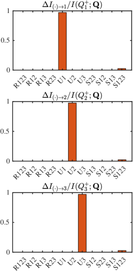
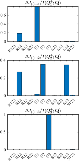
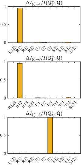
Figure 20: Redundant (R), unique (U) and synergistic (S) causalities for $Q_{1}$, $Q_{2}$, $Q_{3}$ in coupled logistic maps for (left panels, in red) uncoupled variables, $c_{12}=0$ and $c_{123}=0$, (center panels, in blue) intermediate coupling $Q_{1}\rightarrow Q_{2}$, $c_{12}=0.1$ and $c_{123}=0$ and (right panels, in yellow) strong coupling $Q_{1}\rightarrow Q_{2}$ $c_{12\rightarrow 3}=1$ and $c_{12\rightarrow 3}=0$.

Next, we consider three additional cases in which $Q_{3}$ is coupled with $Q_{1}$ and $Q_{2}$. The results are shown in figure 21.

• Strong coupling $Q_{2},Q_{1}\rightarrow Q_{3}$ and no coupling $Q_{1}\rightarrow Q_{2}$ ($c_{12\rightarrow 3}=0$ and $c_{123\rightarrow 3}=1$). The results, included in the left panels of figure 21 (red bars), show that most of the causality to $Q_{1}$ and $Q_{2}$ is self-induced and unique ($\Delta I^{U}_{1\rightarrow 1}\neq 0$ and $\Delta I^{U}_{2\rightarrow 2}\neq 0$, respectively), with a small redundant contribution from $Q_{3}$. This is consistent the fact that the dynamics of $Q_{1}$ and $Q_{2}$ do not depend on any other variable than themselves, but $Q_{3}$ is coupled with $Q_{1}$ and $Q_{2}$, which results in small amount of redundant causality. There is a strong causality from $Q_{1}$ and $Q_{2}$ to $Q_{3}$ in the form of synergistic causality, being $\Delta I^{S}_{123\rightarrow 3}$ the dominant component consistent with the coupling term $f_{123}$.

• Intermediate coupling $Q_{2},Q_{1}\rightarrow Q_{3}$ and $Q_{1}\rightarrow Q_{2}$ ($c_{12\rightarrow 3}=c_{123\rightarrow 3}=0.1$). This is the most complex scenario since the variables do not synchronize yet they affect each other notably. The results are shown in the center panels of figure 21 (blue bars). The causalities to $Q_{1}$ remain mostly independent from $Q_{2}$ and $Q_{3}$ except for the expected small redundant causalities. The causalities to $Q_{2}$ and $Q_{3}$ exhibit a much richer behavior, with multiple redundant and synergistic causalities. The fact that $Q_{2}$ is not coupled to $Q_{3}$ can be seen from the lack of unique causality $\Delta I^{U}_{3\rightarrow 2}$.

• Strong coupling $Q_{2},Q_{1}\rightarrow Q_{3}$ and $Q_{1}\rightarrow Q_{2}$ ($c_{12\rightarrow 3}=1$ and $c_{123\rightarrow 3}=1$). In this case, the three variables synchronize such that $\Delta I^{R}_{123\rightarrow 1}=\Delta I^{R}_{123\rightarrow 2}=\Delta I^{R}_{123\rightarrow 3}\neq 0$ (i.e., they can be interpreted as exact copies of each other). The results are shown in right panels of figure 21 (yellow bars).

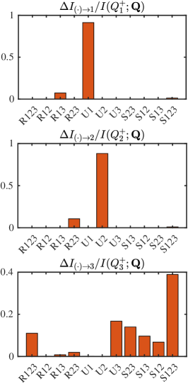
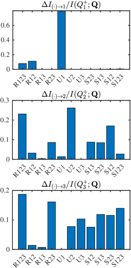
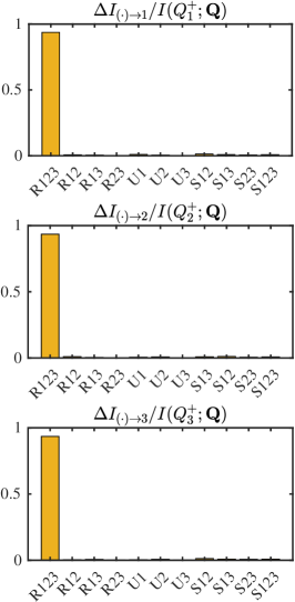
Figure 21: Redundant (R), unique (U) and synergistic (S) causalities for $Q_{1}$, $Q_{2}$, $Q_{3}$ in coupled logistic maps for (left panels, in red) uncoupled variables, $c_{12}=0$ and $c_{123}=1$, (center panels, in blue) intermediate coupling $Q_{1}\rightarrow Q_{2}$, $c_{12}=0.1$ and $c_{123}=0.1$ and (right panels, in yellow) strong coupling $Q_{1}\rightarrow Q_{2}$, $c_{12\rightarrow 3}=1$ and $c_{12\rightarrow 3}=1$.

B.2 Example in coupled Rössler-Lorenz system

We study a coupled version of the Lorenz system (Lorenz, 1963) and the Rössler system (Rössler, 1977). The former was developed by Lorenz as a simplified model of viscous fluid flow. Rössler proposed a simpler version of the Lorenz’s equations in order to facilitate the study its chaotic properties. The governing equations are

$$\frac{{\,\rm{d}}Q_{1}}{{\,\rm{d}}t} =-6[Q_{2}+Q_{3}],$$ (34a)

$$\frac{{\,\rm{d}}Q_{2}}{{\,\rm{d}}t} =6[Q_{1}+0.2Q_{2}],$$ (34b)

$$\frac{{\,\rm{d}}Q_{3}}{{\,\rm{d}}t} =6\left[0.2+Q_{3}[Q_{1}-5.7]\right],$$ (34c)

$$\frac{{\,\rm{d}}Q_{4}}{{\,\rm{d}}t} =10[Q_{5}-Q_{4}],$$ (34d)

$$\frac{{\,\rm{d}}Q_{5}}{{\,\rm{d}}t} =Q_{4}[28-Q_{6}]-Q_{5}+cQ_{2}^{2},$$ (34e)

$$\frac{{\,\rm{d}}Q_{6}}{{\,\rm{d}}t} =Q_{4}Q_{5}-\frac{8}{3}Q_{6},$$ (34f)

where $[Q_{1},Q_{2},Q_{3}]$ correspond to the Rössler system and $[Q_{4},Q_{5},Q_{6}]$ to the Lorenz system. The coupling is unidirectional from the Rössler system to the Lorenz system via $Q_{2}\rightarrow Q_{5}$ and the parameter $c$. This coupled system has previously been studied by Quiroga et al. (2000) and Krakovská et al. (2018).

We use this case to study the behavior of IT-causality among four variables in a continuous dynamical system when some of the variables are hidden. The observable variables are $\boldsymbol{Q}=[Q_{1},Q_{2},Q_{5},Q_{6}]$. The system was integrated for $10^{6}t_{\text{ref}}$ where $t_{\text{ref}}$ is the time-lag for which $I(Q_{1}^{+};Q_{1})/I(Q_{1};Q_{1})=0.5$. The time-lag selected for causal inference is $\Delta T\approx t_{\text{ref}}$ and the 50 bins per variable were used to partition the phase space.

The results for uncoupled systems ($c=0$) are shown in figure 22. The left panel portrays a typical trajectories of the systems. The causalities are shown in the right panel, where red and blue colors are used to represent causalities exclusive to the Rössler system (i.e., only involving $Q_{1}$ and $Q_{2}$) and Lorenz system (i.e., only involving $Q_{5}$ and $Q_{6}$), respectively. Unsurprisingly, IT-causality shows that both systems are uncoupled. Moreover, the unique, redundant and synergistic causal structure identified in the Rössler and Lorenz systems are consistent with structure of Eq. (34a). The information leak is roughly 25% due to the unobserved variables and the uncertainty introduced by partitioning the observable phase-space.

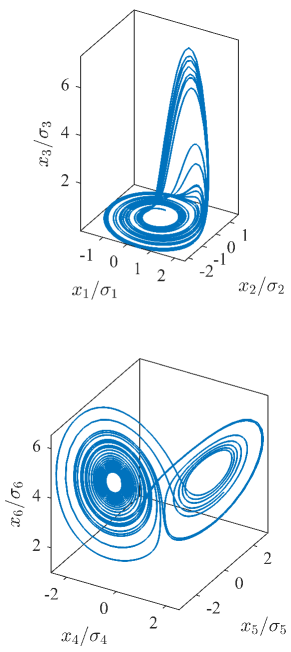
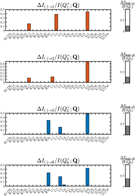
Figure 22: Uncoupled Rössler-Lorenz system ($c=0$). The left panels show excerpts of the trajectories pertaining to Rössler systems $[Q_{1},Q_{2},Q_{3}]$ (top) and Lorenz system $[Q_{4},Q_{5},Q_{6}]$ (bottom). The right panels show the redundant (R), unique (U), and synergistic (S) causalities among $[Q_{1},Q_{3},Q_{4},Q_{6}]$. The causalities are ordered from left to right according to $N_{\boldsymbol{i}\rightarrow j}^{\alpha}$.

The results for the coupled system ($c=2$) are shown in figure 23. The left panel shows how the trajectory of the Lorenz system is severely impacted by the coupling. The new causalities are shown in the right panel. As before, red and blue colors are used to represent causalities exclusive to the Rössler system (i.e., only involving $Q_{1}$ and $Q_{2}$) and Lorenz system (i.e., only involving $Q_{5}$ and $Q_{6}$), respectively, and yellow color is used for causalities involving variables from both systems. The causalities in the Rössler remain comparable to the uncoupled case besides some small redundancies and synergies due to the effect of unobserved variables. On the contrary, the causalities in the Lorenz system undergo deeper changes. This is evidenced by the emergence of multiple synergistic causalities involving $Q_{1}$ and $Q_{2}$. This effect is consistent with the coupling of both systems. The emergence of new redundant and synergistic causalities can be understood as a more complex manifestation of the effect seen in the toy problem from figure 5: the combination of variables yields the creation of redundancies synergies, where the latter dominate.

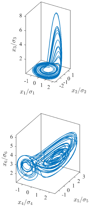
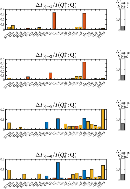
Figure 23: Coupled Rössler-Lorenz system ($c=2$). The left panels show excerpts of the trajectories pertaining to Rössler systems $[Q_{1},Q_{2},Q_{3}]$ (top) and Lorenz system $[Q_{4},Q_{5},Q_{6}]$ (bottom). The right panels show the redundant (R), unique (U), and synergistic (S) causalities among $[Q_{1},Q_{3},Q_{4},Q_{6}]$. The information leak for each variable is also shown in the right-hand side bar. The causalities are ordered from left to right according to $N_{\boldsymbol{i}\rightarrow j}^{\alpha}$.

Appendix C Sensitivity of IT-causality to sample size and partition refinement

We investigate the sensitivity of IT-causality to the number of samples ($N_{\text{samples}}$) used to estimate the probability distributions and the number of bins employed to partition the range of values of the variables ($N_{\text{bins}}$). The Lorenz system is used as a testbed:

$$\frac{{\,\rm{d}}Q_{1}}{{\,\rm{d}}t} =10[Q_{2}-Q_{1}],$$ (35a)

$$\frac{{\,\rm{d}}Q_{2}}{{\,\rm{d}}t} =Q_{1}[28-Q_{3}]-Q_{2}$$ (35b)

$$\frac{{\,\rm{d}}Q_{3}}{{\,\rm{d}}t} =Q_{1}Q_{2}-\frac{8}{3}Q_{3}.$$ (35c)

The system was integrated over time to collect $N_{\text{samples}}=5\times 10^{3},5\times 10^{4},5\times 10^{5},$ and $5\times 10^{8}$ events after transients. Probability distributions were calculated using uniform bins with $N_{\text{bins}}=10,50,100,$ and 200 per variable. Our primary focus is on causalities to $Q_{1}$, but the conclusions drawn also apply to $Q_{2}$ and $Q_{3}$.

The sensitivity to $N_{\text{samples}}$ is displayed in figure 24(a), where $N_{\text{samples}}$ varies while maintaining $N_{\text{bins}}=50$ constant. For $N_{\text{samples}}>5\times 10^{3}$, the changes in IT-causality remain within a few percentage points of difference. The sensitivity to the size of the partition is assessed in figure 24(b), where $N_{\text{bins}}$ varies while $N_{\text{samples}}$ is held constant at $N_{\text{samples}}=5\times 10^{5}$. The IT-causalities exhibit quantitative resemblance for all partitions, with the exception of $N_{\text{bins}}=10$, which may be too coarse to capture the continuous dynamics of the variables.

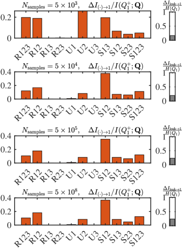
(a)

(b)

Figure 24: Sensitivity of IT-causality in the Lorenz system for (a) number of samples $N_{\text{samples}}$ used to estimate the probability distributions for $N_{\text{bins}}=50$ held constant and (b) the number of bins $N_{\text{bins}}$ used to partition values of the variables for $N_{\text{samples}}=10^{5}$. The causalities are ordered from left to right according to $N_{\boldsymbol{i}\rightarrow 1}^{\alpha}$.

References

- Agostini & Leschziner (2014) Agostini, L. & Leschziner, M. 2014 On the influence of outer large-scale structures on near-wall turbulence in channel flow. Phys. Fluids 26 (7), 075107.
- Agostini & Leschziner (2016) Agostini, Lionel & Leschziner, Michael 2016 Predicting the response of small-scale near-wall turbulence to large-scale outer motions. Phys. Fluids 28 (1).
- Agostini & Leschziner (2022) Agostini, Lionel & Leschziner, Michael 2022 Auto-encoder-assisted analysis of amplitude and wavelength modulation of near-wall turbulence by outer large-scale structures in channel flow at friction reynolds number of 5200. Phys. Fluids 34 (11).
- Altman & Krzywinski (2015) Altman, Naomi & Krzywinski, Martin 2015 Association, correlation and causation. Nature Methods 12 (10), 899–900.
- Aluie & Eyink (2009) Aluie, Hussein & Eyink, Gregory L 2009 Localness of energy cascade in hydrodynamic turbulence. ii. sharp spectral filter. Phys. Fluids 21 (11), 115108.
- Aoyama et al. (2005) Aoyama, T., Ishihara, T., Kaneda, Y., Yokokawa, M., Itakura, K. & Uno, A. 2005 Statistics of energy transfer in high-resolution direct numerical simulation of turbulence in a periodic box. J. Phys. Soc. Jpn. 74, 3202–3212.
- Arnhold et al. (1999) Arnhold, J., Grassberger, P., Lehnertz, K. & Elger, C. E. 1999 A robust method for detecting interdependences: application to intracranially recorded eeg. Phys. D Nonlinear Phenom. 134, 419–430.
- Ballouz & Ouellette (2018) Ballouz, J. G. & Ouellette, N. T. 2018 Tensor geometry in the turbulent cascade. J. Fluid Mech. 835, 1048–1064.
- Beebee et al. (2012) Beebee, H., Hitchcock, C. & Menzies, P. 2012 The Oxford Handbook of Causation. OUP Oxford.
- Bodenschatz (2015) Bodenschatz, E. 2015 Clouds resolved. Science 350 (6256), 40–41.
- Bunge (2017) Bunge, Mario 2017 Causality and modern science. Routledge.
- Busse & Sandham (2012) Busse, B. & Sandham, A. 2012 Parametric forcing approach to rough-wall turbulent channel flow. J. Fluid Mech. 712, 169–202.
- Cambon & Scott (1999) Cambon, Claude & Scott, Julian F. 1999 Linear and nonlinear models of anisotropic turbulence. Annu. Rev. Fluid Mech. 31 (1), 1–53.
- Camps-Valls et al. (2023) Camps-Valls, Gustau, Gerhardus, Andreas, Ninad, Urmi, Varando, Gherardo, Martius, Georg, Balaguer-Ballester, Emili, Vinuesa, Ricardo, Diaz, Emiliano, Zanna, Laure & Runge, Jakob 2023 Discovering causal relations and equations from data. arXiv preprint arXiv:2305.13341 .
- Cardesa et al. (2015) Cardesa, J. I., Vela-Martín, A., Dong, S. & Jiménez, J. 2015 The temporal evolution of the energy flux across scales in homogeneous turbulence. Phys. Fluids 27 (11), 111702.
- Cardesa et al. (2017) Cardesa, J. I., Vela-Martín, A. & Jiménez, J. 2017 The turbulent cascade in five dimensions. Science 357 (6353), 782–784.
- Cheng et al. (2019) Cheng, C., Li, W., Lozano-Durán, A. & Liu, H. 2019 Identity of attached eddies in turbulent channel flows with bidimensional empirical mode decomposition. J. Fluid Mech. 870, 1037–1071.
- Choi & Moin (1990) Choi, H. & Moin, P. 1990 On the space-time characteristics of wall-pressure fluctuations. Phys. Fluids 2 (8), 1450–1460.
- Chung et al. (2014) Chung, D., Monty, J. P. & Ooi, A. 2014 An idealised assessment of townsend’s outer-layer similarity hypothesis for wall turbulence. J. Fluid Mech. 742.
- Cover & Thomas (2006) Cover, T. M. & Thomas, J. A. 2006 Elements of Information Theory. USA: Wiley-Interscience.
- DeWeese & Meister (1999) DeWeese, Michael R & Meister, Markus 1999 How to measure the information gained from one symbol. Network: Computation in Neural Systems 10 (4), 325.
- Diego et al. (2019) Diego, David, Haaga, Kristian Agasøster & Hannisdal, Bjarte 2019 Transfer entropy computation using the perron-frobenius operator. Phys. Rev. E 99 (4), 042212.
- Domaradzki & Rogallo (1990) Domaradzki, J Andrzej & Rogallo, Robert S 1990 Local energy transfer and nonlocal interactions in homogeneous, isotropic turbulence. Phys. Fluids 2 (3), 413–426.
- Domaradzki et al. (2009) Domaradzki, J Andrzej, Teaca, Bogdan & Carati, Daniele 2009 Locality properties of the energy flux in turbulence. Phys. Fluids 21 (2), 025106.
- Eberhardt & Scheines (2007) Eberhardt, Frederick & Scheines, Richard 2007 Interventions and causal inference. Philosophy of science 74 (5), 981–995.
- Eichler (2013) Eichler, M. 2013 Causal inference with multiple time series: principles and problems. Philos. Trans. R. Soc. A-Math. Phys. Eng. Sci. 371 (1997), 20110613.
- Eyink (1995) Eyink, Gregory L 1995 Local energy flux and the refined similarity hypothesis. J. Stat. Phys. 78, 335–351.
- Eyink (2005) Eyink, Gregory L 2005 Locality of turbulent cascades. Phys. D: Nonlinear Phenomena 207 (1-2), 91–116.
- Eyink & Aluie (2009) Eyink, Gregory L & Aluie, Hussein 2009 Localness of energy cascade in hydrodynamic turbulence. i. smooth coarse graining. Phys. Fluids 21 (11), 115107.
- Falkovich (2009) Falkovich, G. 2009 Symmetries of the turbulent state. J. Phys. A 42 (12), 123001.
- Farrell et al. (2017) Farrell, Brian F., Ioannou, Petros J. & Nikolaidis, Marios-Andreas 2017 Instability of the roll-streak structure induced by background turbulence in pretransitional Couette flow. Phys. Rev. Fluids 2, 034607.
- Fiscaletti et al. (2015) Fiscaletti, Daniele, Ganapathisubramani, Bharathram & Elsinga, GE 2015 Amplitude and frequency modulation of the small scales in a jet. J. Fluid Mech. 772, 756–783.
- Flack et al. (2005) Flack, K. A., Schultz, M. P. & Shapiro, T. A. 2005 Experimental support for townsend’s reynolds number similarity hypothesis on rough walls. Phys. Fluids 17, 035102.
- Flores & Jiménez (2006) Flores, O. & Jiménez, J. 2006 Effect of wall-boundary disturbances on turbulent channel flows. J. Fluid Mech. 566 (566), 357–376.
- Granger (1969) Granger, C. W. J. 1969 Investigating causal relations by econometric models and cross-spectral methods. Econometrica pp. 424–438.
- Griffith & Ho (2015) Griffith, Virgil & Ho, Tracey 2015 Quantifying redundant information in predicting a target random variable. Entropy 17 (7), 4644–4653.
- Griffith & Koch (2014) Griffith, Virgil & Koch, Christof 2014 Quantifying synergistic mutual information. In Guided self-organization: inception, pp. 159–190. Springer.
- Gutknecht et al. (2021) Gutknecht, Aaron J, Wibral, Michael & Makkeh, Abdullah 2021 Bits and pieces: Understanding information decomposition from part-whole relationships and formal logic. Proceedings of the Royal Society A 477 (2251), 20210110.
- Haller (2015) Haller, George 2015 Lagrangian coherent structures. Annu. Rev. Fluid Mech. 47 (1), 137–162.
- He et al. (2017) He, G., Jin, G. & Yang, Y. 2017 Space-time correlations and dynamic coupling in turbulent flows. Annu. Rev. Fluid Mech. 49 (1), 51–70.
- Hof et al. (2010) Hof, B., De Lozar, A., Avila, M., Tu, X. & Schneider, T. M. 2010 Eliminating turbulence in spatially intermittent flows. Science 327 (5972), 1491–1494.
- Howland & Yang (2018) Howland, M. F. & Yang, X. I. A. 2018 Dependence of small-scale energetics on large scales in turbulent flows. J. Fluid Mech. 852, 641–662.
- Huang et al. (1998) Huang, Norden E, Shen, Zheng, Long, Steven R, Wu, Manli C, Shih, Hsing H, Zheng, Quanan, Yen, Nai-Chyuan, Tung, Chi Chao & Liu, Henry H 1998 The empirical mode decomposition and the hilbert spectrum for nonlinear and non-stationary time series analysis. In Proc. Royal Soc. Lond., , vol. 454, pp. 903–995. The Royal Society.
- Hutchins & Marusic (2007) Hutchins, Nicholas & Marusic, Ivan 2007 Evidence of very long meandering features in the logarithmic region of turbulent boundary layers. J. Fluid Mech. 579, 1–28.
- Hwang & Cossu (2010) Hwang, Y. & Cossu, C. 2010 Self-sustained process at large scales in turbulent channel flow. Phys. Rev. Lett. 105, 044505.
- Imbens & Rubin (2015) Imbens, G. & Rubin, D. 2015 Causal Inference in Statistics, Social, and Biomedical Sciences. New York, NY, USA: Cambridge University Press.
- Ince (2017) Ince, Robin AA 2017 Measuring multivariate redundant information with pointwise common change in surprisal. Entropy 19 (7), 318.
- Jiménez (2012) Jiménez, J. 2012 Cascades in wall-bounded turbulence. Annu. Rev. Fluid Mech. 44, 27–45.
- Jiménez (2018) Jiménez, J. 2018 Coherent structures in wall-bounded turbulence. J. Fluid Mech. 842, P1.
- Jiménez (2023) Jiménez, Javier 2023 A perron–frobenius analysis of wall-bounded turbulence. J. Fluid Mech. 968, A10.
- Jiménez & Moin (1991) Jiménez, J. & Moin, P. 1991 The minimal flow unit in near-wall turbulence. J. Fluid Mech. 225, 213–240.
- Jiménez & Pinelli (1999) Jiménez, J. & Pinelli, A. 1999 The autonomous cycle of near-wall turbulence. J. Fluid Mech. 389, 335–359.
- de Kat & Ganapathisubramani (2015) de Kat, R. & Ganapathisubramani, B. 2015 Frequency–wavenumber mapping in turbulent shear flows. J. Fluid Mech. 783, 166–190.
- Kawahara et al. (2012) Kawahara, G., Uhlmann, M. & van Veen, L. 2012 The significance of simple invariant solutions in turbulent flows. Annu. Rev. Fluid Mech. 44 (1), 203–225.
- Kolchinsky (2022) Kolchinsky, Artemy 2022 A novel approach to the partial information decomposition. Entropy 24 (3), 403.
- Koller & Friedman (2009) Koller, D. & Friedman, N. 2009 Probabilistic Graphical Models: Principles and Techniques. Cambridge, MA: MIT Press.
- Kolmogorov (1941) Kolmogorov, A. N. 1941 The Local Structure of Turbulence in Incompressible Viscous Fluid for Very Large Reynolds’ Numbers. In Dokl. Akad. Nauk SSSR, , vol. 30, pp. 301–305.
- Kolmogorov (1962) Kolmogorov, A. N. 1962 A refinement of previous hypotheses concerning the local structure of turbulence in a viscous incompressible fluid at high Reynolds number. J. Fluid Mech. 13 (1), 82–85.
- Krakovská et al. (2018) Krakovská, Anna, Jakubík, Jozef, Chvosteková, Martina, Coufal, David, Jajcay, Nikola & Paluš, Milan 2018 Comparison of six methods for the detection of causality in a bivariate time series. Phys. Rev. E 97, 042207.
- Kramer (1998) Kramer, G. 1998 Directed information for channels with feedback. PhD thesis, ETH Zürich.
- Kühnen et al. (2018) Kühnen, J., Song, B., Scarselli, D., Budanur, N. B., Riedl, M., Willis, A. P., Avila, M. & Hof, B. 2018 Destabilizing turbulence in pipe flow. Nat. Phys. 14 (4), 386–390.
- Kullback & Leibler (1951) Kullback, S. & Leibler, R. A. 1951 On information and sufficiency. Ann. Math. Stat. 22 (1), 79–86.
- Liang & Kleeman (2006) Liang, X. S. & Kleeman, R. 2006 Information transfer between dynamical system components. Phys. Rev. Lett. 95, 244101.
- Liang & Lozano-Durán (2016) Liang, X. S. & Lozano-Durán, A. 2016 A preliminary study of the causal structure in fully developed near-wall turbulence. CTR - Proc. Summer Prog. pp. 233–242.
- Lorenz (1963) Lorenz, Edward N 1963 Deterministic nonperiodic flow. J. Atmos. Sci. 20 (2), 130–141.
- Lozano-Durán & Arranz (2022) Lozano-Durán, Adrián & Arranz, Gonzalo 2022 Information-theoretic formulation of dynamical systems: Causality, modeling, and control. Phys. Rev. Res. 4, 023195.
- Lozano-Durán & Bae (2019) Lozano-Durán, A. & Bae, H. J. 2019 Characteristic scales of Townsend’s wall-attached eddies. J. Fluid Mech. 868, 698–725.
- Lozano-Durán et al. (2019) Lozano-Durán, A., Bae, H. J. & Encinar, M. P. 2019 Causality of energy-containing eddies in wall turbulence. J. Fluid Mech. 882, A2.
- Lozano-Durán et al. (2021) Lozano-Durán, Adrián, Constantinou, Navid C., Nikolaidis, Marios-Andreas & Karp, Michael 2021 Cause-and-effect of linear mechanisms sustaining wall turbulence. J. Fluid Mech. 914, A8.
- Lozano-Durán & Jiménez (2014) Lozano-Durán, A. & Jiménez, J. 2014 Effect of the computational domain on direct simulations of turbulent channels up to . Phys. Fluids 26 (1), 011702.
- Martínez-Sánchez et al. (2023) Martínez-Sánchez, Álvaro, López, Esteban, Le Clainche, Soledad, Lozano-Durán, Adrián, Srivastava, Ankit & Vinuesa, Ricardo 2023 Causality analysis of large-scale structures in the flow around a wall-mounted square cylinder. J. Fluid Mech. 967, A1.
- Marusic et al. (2010) Marusic, I., Mathis, R. & Hutchins, N. 2010 Predictive model for wall-bounded turbulent flow. Science 329 (5988), 193–196.
- Marusic & Monty (2019) Marusic, Ivan & Monty, Jason P 2019 Attached eddy model of wall turbulence. Annu. Rev. Fluid Mech. 51, 49–74.
- Massey (1990) Massey, J. 1990 Causality, feedback and directed information. In Proc. Int. Symp. Inf. Theory Applic.(ISITA-90), pp. 303–305. Citeseer.
- Materassi et al. (2014) Materassi, M., Consolini, G., Smith, N. & De Marco, R. 2014 Information theory analysis of cascading process in a synthetic model of fluid turbulence. Entropy 16 (3), 1272–1286.
- Mathis et al. (2009) Mathis, Romain, Hutchins, Nicholas & Marusic, Ivan 2009 Large-scale amplitude modulation of the small-scale structures in turbulent boundary layers. J. Fluid Mech. 628, 311–337.
- Mathis et al. (2011) Mathis, Romain, Marusic, Ivan, Hutchins, Nicholas & Sreenivasan, KR 2011 The relationship between the velocity skewness and the amplitude modulation of the small scale by the large scale in turbulent boundary layers. Phys. Fluids 23 (12).
- May (1976) May, Robert M 1976 Simple mathematical models with very complicated dynamics. Nature 261 (5560), 459–467.
- Mezić (2013) Mezić, I. 2013 Analysis of fluid flows via spectral properties of the koopman operator. Annu. Rev. Fluid Mech. 45 (1), 357–378.
- Mininni et al. (2006) Mininni, PD, Alexakis, A & Pouquet, Annick 2006 Large-scale flow effects, energy transfer, and self-similarity on turbulence. Phys. Rev. E 74 (1), 016303.
- Mininni et al. (2008) Mininni, Pablo Daniel, Alexakis, A & Pouquet, A 2008 Nonlocal interactions in hydrodynamic turbulence at high reynolds numbers: The slow emergence of scaling laws. Phys. Rev. E 77 (3), 036306.
- Mizuno & Jiménez (2013) Mizuno, Y. & Jiménez, J. 2013 Wall turbulence without walls. J. Fluid Mech. 723, 429–455.
- Obukhov (1941) Obukhov, A. M. 1941 On the distribution of energy in the spectrum of turbulent flow. Izv. Akad. Nauk USSR, Ser. Geogr. Geofiz. 5 (4), 453–466.
- Pearl (2000) Pearl, J. 2000 Causality: Models, Reasoning, and Inference. New York, NY, USA: Cambridge University Press.
- Pearl (2009) Pearl, J. 2009 Causality: Models, Reasoning and Inference, 2nd edn. New York, NY, USA: Cambridge University Press.
- Pearson (1895) Pearson, Karl 1895 Vii. note on regression and inheritance in the case of two parents. Proceedings of the royal society of London 58 (347-352), 240–242.
- Pope (2000) Pope, S. B. 2000 Turbulent Flows. Cambridge University Press.
- Quiroga et al. (2000) Quiroga, R. Quian, Arnhold, J. & Grassberger, P. 2000 Learning driver-response relationships from synchronization patterns. Phys. Rev. E 61, 5142–5148.
- Reed et al. (1996) Reed, H L, Saric, W S & Arnal, D 1996 Linear stability theory applied to boundary layers. Annu. Rev. Fluid Mech. 28 (1), 389–428.
- Richardson (1922) Richardson, L. F. 1922 Weather Prediction by Numerical Process. Cambridge University Press.
- Robinson (1991) Robinson, S K 1991 Coherent motions in the turbulent boundary layer. Annu. Rev. Fluid Mech. 23 (1), 601–639.
- Rosales & Meneveau (2005) Rosales, C. & Meneveau, C. 2005 Linear forcing in numerical simulations of isotropic turbulence: Physical space implementations and convergence properties. Phys. Fluids 17 (9), 095106.
- Rössler (1977) Rössler, Otto E 1977 Continuous chaos. In Synergetics: A Workshop Proceedings of the International Workshop on Synergetics at Schloss Elmau, Bavaria, May 2–7, 1977, pp. 184–197. Springer.
- Rubin (1974) Rubin, D. B. 1974 Estimating causal effects of treatments in randomized and nonrandomized studies. J. Educ. Psychol. 66, 688–701.
- Runge (2018) Runge, J. 2018 Causal network reconstruction from time series: from theoretical assumptions to practical estimation. Chaos Interdiscip. J. Nonlinear Sci. 28, 075310.
- Runge et al. (2019) Runge, Jakob, Bathiany, Sebastian, Bollt, Erik & et al. 2019 Inferring causation from time series in earth system sciences. Nat Commun 10, 2553.
- Runge et al. (2018) Runge, J., Nowack, P., Kretschmer, M., Flaxman, S. & Sejdinovic, D. 2018 Detecting causal associations in large nonlinear time series datasets. arXiv:1702.07007v2 [stat.ME] .
- Schmid (2007) Schmid, P. J. 2007 Nonmodal stability theory. Annu. Rev. Fluid Mech. 39 (1), 129–162.
- Schreiber (2000) Schreiber, T. 2000 Measuring information transfer. Phys. Rev. Lett. 85, 461.
- Shannon (1948) Shannon, C. E. 1948 A mathematical theory of communication. Bell Syst. Tech. J 27 (3), 379–423.
- Sinha & Vaidya (2016) Sinha, S. & Vaidya, U. 2016 Causality preserving information transfer measure for control dynamical system. In IEEE 55th Conference on Decision and Control (CDC), pp. 7329–7334.
- Sirovich & Karlsson (1997) Sirovich, L. & Karlsson, S. 1997 Turbulent drag reduction by passive mechanisms. Nature 388, 753–755.
- Smits et al. (2011) Smits, A. J., McKeon, B. J. & Marusic, I. 2011 High-Reynolds number wall turbulence. Annu. Rev. Fluid Mech. 43 (1), 353–375.
- Spearman (1987) Spearman, C. 1987 The proof and measurement of association between two things. The American Journal of Psychology 100 (3/4), 441–471.
- Spirtes et al. (2000) Spirtes, P., Glymour, C. & Scheines, R. 2000 Causation, Prediction, and Search. Cambridge, MA, USA: MIT Press.
- Stone (2013) Stone, J. V. 2013 Information Theory: A Tutorial Introduction.
- Sugihara et al. (2012) Sugihara, G., May, R., Ye, H., Hsieh, C., Deyle, E., Fogarty, M. & Munch, S. 2012 Detecting causality in complex ecosystems. Science 338 (6106), 496–500.
- Tissot et al. (2014) Tissot, G., Lozano-Durán, A., Jiménez, J., Cordier, L. & Noack, B. R. 2014 Granger causality in wall-bounded turbulence. J. Phys. Conf. Ser 506 (1), 012006.
- Torroja (2021) Torroja 2021 Turbulent flow databases. https://torroja.dmt.upm.es/turbdata/, [Online; accessed April-2021].
- Towne et al. (2023) Towne, Aaron, Dawson, Scott T. M., Brès, Guillaume A., Lozano-Durán, Adrián, Saxton-Fox, Theresa, Parthasarathy, Aadhy, Jones, Anya R., Biler, Hulya, Yeh, Chi-An, Patel, Het D. & Taira, Kunihiko 2023 A database for reduced-complexity modeling of fluid flows. AIAA J. 61 (7), 2867–2892.
- Townsend (1976) Townsend, A. A. 1976 The structure of turbulent shear flow. Cambridge University Press.
- Veynante & Vervisch (2002) Veynante, D. & Vervisch, L. 2002 Turbulent combustion modeling. Prog. Energy Combust. Sci. 28 (3), 193–266.
- Wallace (2016) Wallace, J.M 2016 Quadrant analysis in turbulence research: history and evolution. Annu. Rev. Fluid Mech. 48, 131–158.
- Wallace (2014) Wallace, J. M. 2014 Space-time correlations in turbulent flow: A review. Theor. Appl. Mech. Lett. 4 (2), 022003.
- Wang et al. (2020) Wang, H.-N., Huang, W.-X. & Xu, C.-X. 2020 Space–time characteristics of turbulence in minimal flow units. Phys. Fluids 32 (12), 125103.
- Wang et al. (2021) Wang, W., Chu, X., Lozano-Durán, A., Helmig, R. & Weigand, B. 2021 Information transfer between turbulent boundary layers and porous media. J. Fluid Mech. 920, A21.
- Wang et al. (2022) Wang, Wenkang, Lozano-Durán, Adrián, Helmig, Rainer & Chu, Xu 2022 Spatial and spectral characteristics of information flux between turbulent boundary layers and porous media. J. Fluid Mech. 949, A16.
- Wiener (1956) Wiener, N. 1956 The theory of prediction, modern mathematics for engineers. McGraw-Hill.
- Wilczek et al. (2015) Wilczek, M., Stevens, R. J. & Meneveau, C. 2015 Spatio-temporal spectra in the logarithmic layer of wall turbulence: large-eddy simulations and simple models. J. Fluid Mech. 769.
- Williams & Beer (2010) Williams, Paul L & Beer, Randall D 2010 Nonnegative decomposition of multivariate information. arXiv preprint arXiv:1004.2515 .
- Young & Read (2017) Young, R. M. B. & Read, P. L. 2017 Forward and inverse kinetic energy cascades in Jupiter’s turbulent weather layer. Nat. Phys. 13, 1135–1140.
- Zhou (1993a) Zhou, Ye 1993a Degrees of locality of energy transfer in the inertial range. Phys. Fluids 5 (5), 1092–1094.
- Zhou (1993b) Zhou, Ye 1993b Interacting scales and energy transfer in isotropic turbulence. Phys. Fluids 5 (10), 2511–2524.